Complex-plane singularity dynamics for blow up in a nonlinear heat equation: analysis and computation
Abstract
Blow-up solutions to a heat equation with spatial periodicity and a quadratic nonlinearity are studied through asymptotic analyses and a variety of numerical methods. The focus is on the dynamics of the singularities in the complexified space domain. Blow up in finite time is caused by these singularities eventually reaching the real axis. The analysis provides a distinction between small and large nonlinear effects, as well as insight into the various time scales on which blow up is approached. It is shown that an ordinary differential equation with quadratic nonlinearity plays a central role in the asymptotic analysis. This equation is studied in detail, including its numerical computation on multiple Riemann sheets, and the far-field solutions are shown to be given at leading order by a Weierstrass elliptic function.
ams
35B44, 32S99, 35C20, 41A21, 65N99, ,
Keywords: Nonlinear blow up; Complex singularities; Matched asymptotic expansions; Fourier spectral methods; Padé approximation
1 Introduction
The nonlinear heat equation (NLH)
| (1) |
is known to exhibit finite-time blow up; see [1, 2, 3, 4, 5] for reviews and Figure 1 for typical solution profiles. The NLH is a model for reaction-diffusion processes and has appeared in numerous applications including fluid dynamics [6, 7, 8], chemical kinetics [9, 10, 11] and biology [12]. The blow-up behaviour of solutions to the NLH and more general nonlinear parabolic PDEs has been studied extensively on the real line; see the previously mentioned review papers as well as [13, 14, 15]. The novel approach of the present paper is to investigate in detail how the blow up relates to singularity dynamics of the solution when it is viewed as an analytic function in the complex plane, with (only the spatial variable is complexified here). We adopt a combination of asymptotic and numerical methods with the goal of obtaining a comprehensive description of the complex-plane behaviour leading to blow up.


The complex-analytic viewpoint for the NLH was introduced in [16], which was inspired by similar approaches to the Burgers equation [17, 18, 19, 20] and the Korteweg–de Vries equation [21]. The particular example of [16] involved a real-valued, -periodic solution in , associated with the initial condition
| (2) |
with only considered in that paper. Here, we consider all and will thus be able to distinguish between initially small and large nonlinear effects.
Viewed in the complex plane, the initial condition (2) is an entire function. For small , singularities are born at infinity and the ones closest to the real axis, which we locate at , rapidly move along the imaginary axis towards the real axis, with real on the imaginary axis for . Figure 2 shows the position of the closest singularity on the positive imaginary axis for the solutions in Figure 1. Since the solution in the upper and lower half planes are equal up to complex conjugation (, ), we shall consider the solution only in the upper half plane.
The singularity dynamics in Figure 2 exemplify the competing effects of diffusion and nonlinearity in the NLH. For large enough , as in the top left frames of Figures 1 and 2, the focussing nonlinear term dominates diffusion in the sense that the singularity approaches the real axis monotonically, albeit not at constant speed. The solution profile on the real axis steepens as the singularity approaches the real axis, with point blow up occurring when the two closest singularities in the upper and lower half planes collide on the real axis. If is small enough, as in the bottom row of Figures 1 and 2, diffusion dominates initially and we see that the solution profile flattens while the singularities reverse direction after zooming in from infinity to move away from the real axis. However, even as the solution flattens, its mean increases11 1 The mean of the solution, , satisfies , as can be derived from (1) using integration by parts. and thus eventually nonlinearity reasserts itself, the solution profile becomes steeper, the singularity changes direction again and rapidly moves towards the real axis and point blow up ensues. For the case in the top-right frame of Figure 2 there is a balance between nonlinearity and diffusion in which the singularity is near stationary for a while after zooming in from infinity and before zooming in again as point blow-up occurs.


With the initial data (2), the solution has a point blow up at for any . The blow up may occur at other points, however, or not at all. For example, note that corresponds to a translation of the solution and thus shifts the blow-up location from the maximum of the initial data (2) at to . On the other hand, we shall also consider
| (3) |
briefly in an appendix. If is sufficiently large negative for a fixed , then the solution does not blow up but extinguishes (‘heat death’ occurs) according to , ; see the left frame of Figure 3. Otherwise, point blow up occurs at (i) if and at (ii) if 22 2 On the (unstable) borderline between blow up and extinction one has as .. For an example of (i), we perturb the initial data of the heat-death solution in Figure 3 and obtain the solution in the right frame of Figure 3. For the heat-death solution, the singularities zoom in from infinity, change direction and then move back (linearly in time, as we shall show) to infinity, see Figure 4. This figure also shows that when perturbing the heat-death solution, the singularities can switch direction a second time and move towards the real axis, which leads to blow up.


In our analysis of the solution in the blow-up limit, we shall also briefly consider the blow-up scenarios, and associated singularity dynamics, for initial data with two local maxima. Figure 5 shows two possibilities: blow up occurs at two distinct points for even initial data with two sufficiently separated and concentrated peaks (left frame) and (right frame) two maxima are sufficiently close to diffuse and combine into a single maximum, and then blow up occurs at a single point. We shall also consider the non-generic blow up that occurs when the two maxima combine precisely at the blow-up time, which represents the borderline between the cases shown in Figure 5.


Other complex-plane studies of the NLH have been reported in [22, 23]. In both papers the equation was studied numerically in the complex -plane. Related studies reported in [24] focused on the case of nearly flat initial data
| (4) |
The properties of blow up were investigated but singularity dynamics in the complex -plane were only mentioned briefly.
The paper consists of seven sections and six appendices, the latter containing the bulk of the more technical analyses. In section 2 we review two numerical approaches based on Fourier analysis for locating and classifying the singularities alluded to above. In section 3 we complement the numerical investigation by a local analysis that characterises the type of singularities admitted by the equation. Sections 4–6 are devoted to the analysis and numerical verification of the dynamics of the singularities and the relation of the NLH solution in the neighbourhood of the singularities to certain nonlinear ODE solutions. The ODE solutions are studied in detail in B. Section 4 and A concern the small-time limit for all amplitudes . Section 5 and C consider the large-amplitude limit, , and section 6 and D treat the small amplitude limit, . As Figures 1 and 2 indicate, the small-amplitude singularity dynamics are the most complicated. This will be borne out by the asymptotic analysis, in which a complete description requires five distinct time scales. To complete our study, in section 7 and E we consider the solution in the blow-up limit. Sections 4–7 focus on NLH solutions subject to the initial data (2) but the final appendix, F, considers NLH solutions corresponding to the more general initial condition (3). Throughout we shall reuse symbols with different meanings in different sections.
2 Numerical method and singularity tracking
The numerical solutions reported in this paper were computed by a Fourier spectral method. Considering solutions -periodic in space, the approximation is based on the Fourier series
| (5) |
When this is substituted into (1) an infinite dynamical system for the evolution of the coefficients is obtained. Upon truncation to modes , a finite-dimensional system is obtained, which we integrated in time with the adaptive time-step functions ode45 and ode15s available in MATLAB. The main advantage of these integrators is the error control that they provide. By experimentation, the number of modes, , was chosen sufficiently large so that all results presented here have fully converged.
For computing solutions close to blow up, a powerful strategy has been suggested in [15] and used in [24]. Namely, the substitution converts (1) into an equivalent PDE whose solution approaches zero rather than infinity at the blow-up point. This method can maintain high accuracy for blow-up solutions for values on the order of , where here denotes the machine precision, which can be made arbitrarily small with variable precision arithmetic but which is approximately for IEEE double precision. In the present paper, we use the Fourier spectral method in the variable whenever is strictly positive, otherwise, if changes sign on , we solve the PDE in the variable. The latter method is accurate for solution values only up to approximately in double precision. If changes sign and arbitrarily large solution values are required then more complicated numerical methods such as domain decomposition, dynamical rescaling and/or adaptive mesh refinement are needed; see [13, 14].
As for singularity tracking, there are two main numerical techniques. The first is based on the examination of the rate of decay of the Fourier coefficients in (5). The other is based on Fourier-Padé methods for numerical analytic continuation.
The first of these methods is described in the well-known paper by Sulem et al. [25]. Suppose at a fixed time the coefficients of the series (5) are available. If the singularity closest to the real axis is at and
| (6) |
for some constant , then [25]
| (7) |
Given values of for a range , the values of and can be estimated by a linear least squares fit, after taking logarithms in (7). The singularity locations shown in Figure 2 were computed by this method.
In the next section we proceed with a theoretical analysis of the singularities of (1), but we assume for now an expression of the form (6). The least-squares procedure then produces the estimates for the exponent shown in Figure 6. These results suggest that the singularities could be poles of order two, except in an intermediate asymptotic sense for initial times and as blow up is approached. The asymptotic analyses in the next sections will clarify these numerical estimates.


The other method for singularity tracking is based on Fourier–Padé methods as considered for the NLH (and other PDEs) in [16]. The Fourier series (5) is converted to rational trigonometric form, which can be continued into the complex plane to some strip around the real axis. The advantage of this method over the method (6)–(7) is that it often gives information further into the complex plane, beyond the singularities closest to the real axis. In a further improvement this method was recently extended to quadratic Fourier–Padé, which incorporates a square-root singularity into the approximant in an attempt to capture branch point singularities more accurately [26].
In Figure 7 we show phase plots for the case , computed by this quadratic Fourier–Padé method. (It provides a different view of the singularity dynamics shown in the third frame of Figure 2.) This improves on the figure given in [16, Fig. 5.2], which was computed with the standard Fourier–Padé approach. By examining the phase plots, it again appears that the dominant singularity is a pole of order two, as was evident in Figure 6 as well. As the singularity approaches the real axis, however, the characteristics of a branch point become evident. The analysis of the next section will clarify this.


3 Local analysis of the singularities
In this section we examine more closely the nature of the singularities described in sections 1 and 2. Locating a singularity in the complex plane at and setting gives
| (8) |
where the dot represents differentiation with respect to . The right-hand side dominates the local behaviour, so that as ,
Setting
and linearising, at leading order the ‘complementary function’ satisfies the Euler equation
so that
Self-consistency requires (this contribution being associated with the -translation-invariance of (8)), but and are arbitrary in terms of the local analysis, representing the two degrees of freedom expected of a generic singularity in this second-order problem. Reinstating the intervening terms in the local expansion about the singularity in (8), one finds that
| (9) |
where
Note that the presence of the term implies that the singularity is actually a branch point. However, the double-pole nature of the dominant term in (9) significantly precedes this in the local expansion. This explains why both singularity tracking methods in section 2 singled out this type of singularity.
The expansion might also explain why the method (6)–(7) suggests simple pole singularities near and near blow up; see Figure 6. This is because the second term on the right in (9) has a residue proportional to , and this value is large initially and again near blow up, as can be confirmed in Figure 2. A more detailed asymptotic analysis is required fully to clarify the matter; see below.
The method based on the quadratic Fourier-Padé method is able, at least ultimately, to classify the singularity as a branch point; see the last frame of Figure 7. The approximant is a two-valued function, so it is unable to capture the logarithmic singularity perfectly, but at least the presence of a branch point is indicated strongly.
4 Small-time limit: singularity dynamics and singularity structure
In the first of our appendices, A, it is shown that for the initial condition (2) and for small values of , the NLH solution on the real axis is
Furthermore, it is shown that the singularity closest to the real axis on the positive imaginary axis is located at , . In the vicinity of , the solution to the NLH in the complex plane is given by
| (10) |
where is the solution to the nonlinear ODE
| (11) |
subject to the asymptotic condition
| (12) |
Let be the first singularity that is encountered on the real axis as the ODE problem (11)–(12) is integrated from , then it follows from (10) that a small-time approximation to the singularity location is given by , where
| (13) |
In subsequent sections, we shall find that the ODE (11) subject to (12) or variations thereof arises repeatedly in our analysis of NLH solutions in the complex plane. Consequently, a detailed analysis of these ODE solutions is given in B.

Figure 8 shows the solution to (11)–(12), revealing that . In B, higher-order terms in the asymptotic expansion (12) are derived in order to compute the initial condition to an accuracy on the order of machine precision. The solution to the ODE (11) is then computed in the complex -plane using the ‘pole field solver,’ a method based on an adaptive Padé one-step method [30, 31].
Figure 9 shows the estimate (13) compared to the numerical estimate of the singularity location described by (6)–(7). Both the graphical and the numerical comparisons confirm that the asymptotic and numerical estimates match well for small . As to be expected, the accuracy of the asymptotic estimate deteriorates as increases.

The asymptotic analysis in A provides another perspective on why the singularity exponent in Figure 6 increases from roughly to as increases from small to intermediate values. It is shown in (41) that in the small-time limit, the leading-order behaviour of the singularity (after a single rescaling) is that of a simple pole. It is this leading-order simple pole nature of the singularity that is detected by the numerical method. It is only after a second rescaling that one arrives at an equation, viz. (44), whose singularity type matches that of the NLH.
The type of singularities admitted by the ODE (11) are (unsurprisingly) of the same type as those of the NLH since if one assumes a singularity of the ODE is located at , then the local expansion takes the form
| (14) |
where is an arbitrary constant. This shows that the ODE (11) does not possess the Painlevé property since it has branch point singularities whose locations are dependent on the initial conditions (i.e., movable branch points). This also confirms that the essential singularity that is present in the initial condition at , and which (9) indicates to be incompatible with the NLH, is transformed for any into singularities of the compatible form (9).
Figure 8 suggests that the branch point singularity at is the only singularity of on the principal Riemann sheet of the solution to (11)–(12). It is also of interest to examine if, and where, other singularities might occur. Integrating clockwise around onto the next Riemann sheet, we obtain the solution shown in Figure 10, which reveals the presence of a multitude of singularities. Such singularities could, at least in principle, subsequently move onto the principal Riemann sheet and influence the real-time behaviour; however, such effects seem not to be of importance in the current context.
B.4 shows that, to leading order, the solution for on the second Riemann sheet is expressible in terms of the (equianharmonic) Weierstrass elliptic function in the variable (see (53) and (56)). Hence, in the bottom frame of Figure 8, we find that in the -plane the far-field singularities on the second Riemann sheet lie approximately on the same lattice as the singularities of the Weierstrass elliptic function.


5 Large-amplitude initial conditions
In C it is shown that for the initial condition (2) with large amplitude, a leading-order approximation to the solution on the real line is, for
| (15) |
Hence, to leading order, the singularity locations are , where
| (16) |
The formula on the right makes it clear that as , this estimate is consistent with the result of the small-time analysis (13). The singularities move along the imaginary axis and collide with the real axis at for . The motion of the singularities is monotonically towards the real axis, albeit not at constant speed. Graphs of the singularity locations as functions of time are shown in Figure 11.
The singularities of (15) are simple poles and therefore (15) ceases to be valid close to the singularities. It is shown in C that in a neighbourhood of the closest singularities,
| (17) |
where is the ODE solution defined by (11)–(12) and the formula
| (18) |
defines . Therefore
| (19) |
where is the location of the first singularity of on the real axis, which, as stated in section 4, is .
5.1 Approach to blow up
As the singularities approach the real axis, i.e. in the double limit , , it follows from (15) that
holds. This might suggest that as blow up is approached, the solution takes the self-similar form,
| (20) |
this representing a classical similarity reduction to the NLH. As is well known, there were early conjectures in related problems that blow-up solutions indeed take such a self-similar form (see e.g., [32, 33]), although in [8] the appropriate logarithmic corrections had already been established for a specific form of nonlinearity; see also [9]. Indeed, it is known that no suitable solution to the resulting ODE in fact exists, see [34, 35].
6 Small-amplitude initial conditions
In D, the NLH solution is analysed for the initial data (2) with and it is found that five different time scales are relevant for the asymptotic analysis. Here we summarise the results on the different time scales. The bottom right frames of Figures 1 and 2 show, respectively, the qualitative behaviour of the solution profile and the singularity dynamics. Figure 12 illustrates that the solution in Figure 1 appears to blow up uniformly but in fact it blows up at the point .

6.1
On the first timescale, the solution on the real axis is given by
| (21) |
This approximation, as well as other asymptotic estimates in the upcoming sections 6.2–6.4, will be compared to numerical results in section 6.6.
The closest singularities are at , where
| (22) |
and is the location of a singularity of a nonlinear backward diffusion PDE (namely, (68)–(69)) whose solution is not known explicitly. However, the limiting behaviour of is found to be (i) as (hence (22) is consistent with (13) as ) and (ii) as becomes large according to , .33 3 The shift arises because (68) implies as , . Here is the location of the first singularity of the following nonlinear ODE problem:
| (23) |
The limiting behaviour (ii) follows because for , the NLH solution in the neighbourhood of the singularity, i.e. for , is
| (24) |
where is the solution to (23).
The left frame of Figure 13 compares the numerically determined singularity location (as described in section 2) and the approximation (22), but with neglected. The right frame of the figure shows the difference between these two quantities, which gives an estimate for . As predicted by the asymptotic analysis, increases from zero and for large and , , where , see the top frame of Figure 14. The latter figure shows that the far-field condition in (23) leads to multiple singularities on the principal Riemann sheet of the ODE solution, in contrast to the solution in Figure 8 corresponding to the condition (12). This suggests that the NLH solution has multiple singularities that in the small-time limit live off its principal Riemann sheet but, for small amplitude and large time, move onto its principal Riemann sheet, a possibility we alluded to above.
B.4 shows that the far-field solution of (23) can also be expressed to leading order in terms of the (equianharmonic) Weierstrass function in the variable . Hence the far-field singularities of the solution in the top frame of Figure 14 lie approximately on the same lattice as the Weierstrass function’s singularities in -plane, as shown in the bottom frame of the figure.

6.2
On the second timescale, the solution on the real axis is
| (25) |
where the leading order estimate of the blow-up time is (see D). For the solution in Figure 12 with , this gives the estimate , while the numerically computed blow-up time is .
Solutions with initial data (2) have a maximum at (see Figure 1) and, as shown in Appendix B of [24], the peak-to-trough height of the maximum satisfies
for even solutions, provided is not close to the blow-up time. Here is a Fourier coefficient of the solution; see (5). From (25) it follows that
| (26) |
which implies the minimum peak-to-trough height of the solution decreases exponentially with . With it follows that , which means that the solution is completely flat in double-precision arithmetic and a uniform blow up is computed. This is incorrect since, as we shall see, point blow up eventually occurs for any . Consequently, higher precision or rescaling methods would be required to compute the solution for . Figure 15 compares the asymptotic estimate (26) to the numerically computed peak-to-trough height and confirms the validity of the estimate away from the blow-up time.
In the neighbourhood of the singularity, i.e. for , the NLH solution is given by
where is again defined as the solution to (23). Hence an estimate of the singularity location is
| (27) |
where is the first singularity of (23) on the real axis, which was found to be in section 6.1. This estimate for , as well as the estimates in the upcoming sections, will be compared to numerical results in section 6.6.
6.3
On this time scale, the solution on the real axis is given again by (25). The singularity location evolves on the imaginary axis according to (cf. (27))
| (28) |
where is the position of the first singularity of another nonlinear backward diffusion PDE initial-value problem ((84)–(85)) whose solution is not known explicitly. However, the limiting behaviour of is shown in D.3 to be as follows: for with , , where is the first singularity of (23) on the real axis, i.e. and therefore (28) tends to (27). For , to leading order and thus
| (29) |
6.4 Fourth time scale
The fourth time scale, which is valid exponentially close to the blow-up time, is defined via
with , and to leading order
| (30) |
Therefore blow up occurs at and the modification to the algebraic expansion for resulting from the previous timescales is the exponentially small, and hence in practice irrelevant quantity
An approximation for the locations of the closest singularities (which will be used in section 6.6) is with
| (31) |
6.5 Fifth time scale
As blow up is approached, , apply in (30) and therefore
This suggests the self-similar form
cf. (20). Again, the appropriate ODE solution fails to exist, which necessitates the introduction of a final (doubly exponentially short) time variable to capture the logarithmic corrections. The approach to blow up is analysed in more detail in E.
6.6 Comparisons to numerical results
Having derived a large number of estimates for the small amplitude case, we now compare some of them to numerical approximations. Figure 16 shows the accuracy of the asymptotic approximations to the solution on the real axis given in (21), (25) and (30) for the case . We note that the need for a comparatively large value of reflects the asymptotic structure whereby the small quantity is prominent: the extent to which becomes near uniform is a striking feature of the analysis. In (25), we choose to be the numerical blow-up time and in (30) we choose such that the blow-up time of (30), namely (i.e., at ), coincides with the numerical blow-up time.
Figure 17 compares the asymptotic estimates of the closest singularities at (see (22), (27), (28), (29) and (31)) to the numerically computed singularity position. For all these asymptotic approximations, we let be the numerically computed blow-up time. For the estimate (27), we use the value of , while for (28), since the function is not known explicitly, we replace and with constants44 4 In Figure 17, these constants are and . and such that the local maximum of the resulting estimate matches that of the numerical singularity position.
7 Blow-up limit
Figure 18 shows a small-amplitude NLH solution at times approaching the blow-up time. Since the solution is even, it is shown only for with . The figure illustrates the well-known fact that, as the blow-up time is approached, the solution is flat for , where ; see E.1. That is, for a fixed with , the solution is flat with for sufficiently small. More precisely, as shown in E.2, for ,
| (32) |
where is a constant that depends on the initial data. This approximation is shown as dotted curves in Figure 18 and matches the numerical solution well for sufficiently small .
As is clear from Figure 18, the solution is asymptotically flat on an interval whose width shrinks to zero as and, as shown in E.3, the solution acquires the blow-up profile,
| (33) |
where the constant is defined in E. This profile is shown as a dashed curve in the right frame of Figure 18, which matches the non-flat part of the numerical solution well for sufficiently small . We note that, before the blow-up time, the closest singularities are second-order poles to leading order with a logarithmic term at fourth order (see (9)); however, in the blow-up limit, the leading-order behaviour for , namely , acquires a logarithmic contribution.
Unlike the asymptotic estimates (32) and (33), the asymptotics of the blow-up profile in [24] are valid on the entire interval (they are -periodic) and the constants are expressed explicitly in terms of the initial data considered in that paper, namely (4). For comparison purposes, we restate the analogue of (32) from [24]: as
| (34) |
where and are parameters in the initial data (4) and
Setting in (34), we obtain
| (35) |
As shown in [24], at the blow-up time and for exponentially small with respect to , the following analogue of (33) holds,
| (36) |
The left frame of Figure 19 shows the accuracy of the asymptotic approximations (34)–(36) and the right frame compares the small-amplitude NLH solution with in Figure 18 with another NLH solution with but subject to the initial data (4).
As discussed in the introduction, for an even initial condition with two local maxima, blow up of the type we have discussed here (generic blow-up) can occur simultaneously at two points (see the left frame of Figure 5) or at a single point (right frame of Figure 5). In the former case, two singularities collide on the real axis at both blow-up points and in the latter case (see Figure 20), a pair of singularities coalesces in each of the upper and lower half-planes before the resulting singularities collide on the real axis at blow-up. The borderline case, in which two singularities from the upper half-plane and two singularities from the lower half-plane collide on the real axis at the same point at the blow-up time (see Figure 21) is a type of non-generic blow up for which the leading-order behaviour at blow up is , , where depends on the initial data. (See E.5 and Figure 22.)


8 Conclusion
For the NLH we have given asymptotic descriptions (along with numerical confirmation) of: its branch-point-type singularities, the solution in the neighbourhood of the closest singularities in the complex plane, the complex-plane dynamics of the closest singularities and the solution in the small-time, large-amplitude, small-amplitude and blow-up limits.
Numerous generalisations suggest themselves; perhaps the most immediate is the quasilinear power-law case
with , , for which the blow-up behaviour is well-known to differ from that for the semilinear case with which we have been concerned here; indeed, the latter can be viewed as the borderline case between two distinct classes of behaviour, the logarithmic terms that are prevalent in the above being associated with this borderline status.
We related the NLH solution to nonlinear ODE solutions (which have interesting properties in their own right) in certain limits and found the singularity locations of the ODE solutions numerically (via the pole field solver) and asymptotically. A possibility for future work would be to develop an analogue of the pole field solver for PDEs. Just as the pole field solver can accurately compute multivalued ODE solutions by using the ODE and adaptive Padé approximation to continue analytically the solution onto multiple Riemann sheets, so a pole field solver for PDEs might be able to compute, for a fixed time , the NLH solution on multiple Riemann sheets in the complex plane. The numerical analytic continuation method for the NLH that we used in this paper (Padé and quadratic Padé approximation using the Fourier expansion of the solution) is accurate in a neighbourhood of the closest singularities of the NLH. However, it rapidly loses accuracy as one moves further away from the real axis. A pole field solver for PDEs would presumably maintain accuracy much further away from the real axis and also onto neighbouring Riemann sheets.
9 Acknowledgements
The authors would like to thank the Isaac Newton Institute for Mathematical Sciences for support and hospitality during the programme Complex analysis: techniques, applications and computations when work on this paper was undertaken. This programme was supported by EPSRC grant number EP/R014604/1. The work of the first author was also supported by the Leverhulme Trust Research Project Grant RPG-2019-144. The second author gratefully acknowledges a Royal Society Leverhulme Trust Senior Fellowship. The third author acknowledges a grant from the H.B. Thom Foundation of Stellenbosch University that enabled participation in the above mentioned programme.
References
References
- [1] C. Bandle, H. Brunner, Blowup in diffusion equations: a survey, J. Comput. Appl. Math. 97 (1-2) (1998) 3–22.
- [2] V. A. Galaktionov, J. Vázquez, The problem of blow-up in nonlinear parabolic equations, Disc. Cont. Dyn. Syst. 8 (2) (2002) 399–433.
- [3] V. Galaktionov, J. Vazquez, Continuation of blowup solutions of nonlinear heat equations in several space dimensions, Commun. Pure Appl. Math 50 (1) (1997) 1–67.
- [4] P. Quittner, P. Souplet, Superlinear Parabolic Problems: Blow-up, Global Existence and Steady States, Springer, 2019.
- [5] A. Samarskii, V. Galaktionov, S. Kurdyumov, A. Mikhailov, Blow-up in Quasilinear Parabolic Equations, Walter de Gruyter, 1995.
- [6] S. Braun, A. Kluwick, Unsteady three-dimensional marginal separation caused by surface-mounted obstacles and/or local suction, J. Fluid Mech. 514 (2004) 121–152.
- [7] S. Braun, A. Kluwick, Blow-up and control of marginally separated boundary layers, Philos. Trans. R. Soc. Lond. Ser. A Math. Phys. Eng. Sci. 363 (1830) (2005) 1057–1067.
- [8] L. Hocking, K. Stewartson, J. Stuart, S. Brown, A nonlinear instability burst in plane parallel flow, J. Fluid Mech. 51 (4) (1972) 705–735.
- [9] J. Dold, On asymptotic forms of reactive-diffusive runaway, Proc. R. Soc. Lond. 433 (1889) (1991) 521–545.
- [10]
M. A. Herrero, J. J. L. Velázquez,
Plane structures in thermal
runaway, Israel J. Math. 81 (3) (1993) 321–341.
doi:10.1007/BF02764836.
URL https://doi.org/10.1007/BF02764836 - [11]
A. A. Lacey, Mathematical analysis of
thermal runaway for spatially inhomogeneous reactions, SIAM J. Appl. Math.
43 (6) (1983) 1350–1366.
doi:10.1137/0143090.
URL https://doi.org/10.1137/0143090 - [12] S. Jabbari, J. King, Discrete and continuum multiscale behaviour in bacterial communication, in: Multiscale Computer Modeling in Biomechanics and Biomedical Engineering, Springer, 2013, pp. 299–320.
- [13]
M. Berger, R. V. Kohn, A
rescaling algorithm for the numerical calculation of blowing-up solutions,
Comm. Pure Appl. Math. 41 (6) (1988) 841–863.
doi:10.1002/cpa.3160410606.
URL https://doi.org/10.1002/cpa.3160410606 - [14] C. Budd, G. Collins, V. Galaktionov, An asymptotic and numerical description of self-similar blow-up in quasilinear parabolic equations, J. Comput. Appl. Math. 97 (1-2) (1998) 51–80.
- [15] J. B. Keller, J. S. Lowengrub, Asymptotic and numerical results for blowing-up solutions to semilinear heat equations, in: Singularities in fluids, plasmas and optics (Heraklion, 1992), Vol. 404 of NATO Adv. Sci. Inst. Ser. C Math. Phys. Sci., Kluwer Acad. Publ., Dordrecht, 1993, pp. 111–129.
- [16] J. Weideman, Computing the dynamics of complex singularities of nonlinear PDEs, SIAM J. Appl. Dyn. Syst. 2 (2003) 171–186.
- [17] D. Bessis, J.-D. Fournier, Complex singularities and the Riemann surface for the Burgers equation, in: Nonlinear physics (Shanghai, 1989), Res. Rep. Phys., Springer, Berlin, 1990, pp. 252–257.
- [18] D. Bessis, J. Fournier, Pole condensation and the Riemann surface associated with a shock in Burgers’ equation, J. Physique Lett. 45 (17) (1984) 833–841.
- [19] D. Senouf, Dynamics and condensation of complex singularities for Burgers’ equation. I, SIAM J. Math. Anal. 28 (6) (1997) 1457–1489.
- [20] D. Senouf, Dynamics and condensation of complex singularities for Burgers’ equation. II, SIAM J. Math. Anal. 28 (6) (1997) 1490–1513.
- [21] M. Kruskal, The Korteweg-de Vries equation and related evolution equations, in: Nonlinear wave motion.(A75-14987 04-70) Providence, RI, American Mathematical Society, 1974, p. 61-83., 1974, pp. 61–83.
- [22] C.-H. Cho, H. Okamoto, M. Shoji, A blow-up problem for a nonlinear heat equation in the complex plane of time, Jpn. J. Ind. Appl. Math. 33 (1) (2016) 145–166.
- [23] A. Takayasu, J. Lessard, J. Jaquette, H. Okamoto, Rigorous numerics for nonlinear heat equations in the complex plane of time, Numer. Math. 151 (3) (2022) 693–750.
- [24] M. Fasondini, J. King, J. Weideman, Blow up in a periodic semilinear heat equation, Physica D: Nonlinear Phenomena 446 (2023) 133660.
- [25] C. Sulem, P. Sulem, H. Frisch, Tracing complex singularities with spectral methods, J. Comput. Phys. 50 (1) (1983) 138–161.
- [26] M. Fasondini, N. Hale, R. Spoerer, J. Weideman, Quadratic Padé approximation: numerical aspects and applications, Computer Research and Modeling 11 (6) (2019) 1017–1031.
- [27] NIST Digital Library of Mathematical Functions, https://dlmf.nist.gov/, Release 1.1.10 of 2023-06-15, f. W. J. Olver, A. B. Olde Daalhuis, D. W. Lozier, B. I. Schneider, R. F. Boisvert, C. W. Clark, B. R. Miller, B. V. Saunders, H. S. Cohl, and M. A. McClain, eds.
- [28] E. Wegert, Visual Complex Functions: an Introduction with Phase Portraits, Springer Science & Business Media, 2012.
- [29] E. Wegert, Phase plots of complex functions, https://www.mathworks.com/matlabcentral/fileexchange/44375-phase-plots-of-complex-functions, MATLAB Central File Exchange. Retrieved July 31, 2023. (2023).
- [30] M. Fasondini, B. Fornberg, J. Weideman, Methods for the computation of the multivalued Painlevé transcendents on their Riemann surfaces, J. Comput. Phys. 344 (2017) 36–50.
- [31] B. Fornberg, J. Weideman, A numerical methodology for the Painlevé equations, J. Comput. Phys. 230 (15) (2011) 5957–5973.
- [32] A. Kapila, Reactive-diffusive system with Arrhenius kinetics: dynamics of ignition, SIAM J. Appl. Math. 39 (1) (1980) 21–36.
- [33] D. Kassoy, J. Poland, The thermal explosion confined by a constant temperature boundary: I—the induction period solution, SIAM J. Appl. Math. 39 (3) (1980) 412–430.
- [34] J. Bebernes, W. Troy, Nonexistence for the Kassoy problem, SIAM J. Math. Anal. 18 (4) (1987) 1157–1162.
- [35] D. Eberly, Nonexistence for the Kassoy problem in dimensions 1 and 2, J. Math. Anal. Appl. 129 (2) (1988) 401–408.
- [36] M. Ablowitz, A. Zeppetella, Explicit solutions of Fisher’s equation for a special wave speed, Bull. Math. Biol. 41 (6) (1979) 835–840.
Appendix A Analysis of the small-time limit
The Taylor expansion of the NLH in with initial condition (2) yields
| (37) |
which holds sufficiently close to the real axis and for small values of . Setting with , the terms and come into balance, leading to a non-uniformity in (37) when , where
| (38) |
Setting , (37) implies the matching condition
| (39) |
In these variables, the NLH becomes
Letting , as with we find that and must satisfy
| (40) |
Given (39), the required solutions are
| (41) |
Note that has a simple pole at , which does not match the type of singularity of the NLH found in section 3, while has a double pole at , which implies a further non-uniformity for small . Since
| (42) |
the resulting inner rescalings are
| (43) |
and, in these variables, the NLH becomes
Setting as with , satisfies
| (44) |
In order to match the behaviour (42) for , we require that satisfies the far-field condition
| (45) |
prescribing the coefficient of the term (which reflects the translation invariance of (45)) specifies uniquely (as can be confirmed by a phase-plane analysis, see Figure 23). Making the change of variables and relabelling , (44)–(45) is equivalent to (11)–(12). Unlike the first equation in (40), the singularities of (44) have the same form as that of the NLH equation, see (14) and (9). Hence, no further rescalings are required. Finally, we note that combining , (38), (43) and , , one obtains (10).
Appendix B A nonlinear ordinary differential equation
The ODE
| (46) |
arises in the analysis of the small-time limit (see (11)), the large-amplitude limit and the small-amplitude limit (see (71) and (80)). Here we elaborate on some of its properties.
B.1 Phase plane
The phase plane of real solutions on the real line is immediately instructive (see the left frame of Figure 23).
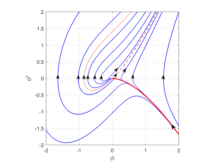
There are precisely three exceptional trajectories, each of which is relevant to our analysis, with the following behaviour:
| (47) |
( is a positive constant),
| (48) |
and
| (49) |
For the latter case, is arbitrary and corresponds to a translation of . Notice that (47) and (49) characterise the solutions that arise in the analysis above (cf. (12), (72) and (80)). The solutions specified by (47)–(49) blow up on the real axis (see the right frane in Figure 23) and in particular the singularities of (47) and (49) on the real line are of interest since these are used in the asymptotic estimates of the NLH singularity locations in (13), (19), (22) and (27).
B.2 Computing asymptotic boundary conditions
To compute initial conditions for the solutions (47) and (49) accurately, we generate higher-order terms in their asymptotic boundary conditions for fixed or , respectively, and truncate the expansion when the first omitted term is below the level of machine precision. For (47), the asymptotic expansion takes the form
where is arbitrary (for the solution we require, (see (23)) and
| (50) |
For (49), the expansion takes the form
| (51) |
Comparing this expansion to the first few terms in (49), one gets
where is arbitrary (for the solution we require, , see (12)) and for , ,
where
Figure 24 gives an example of the number of terms of (51) that is required to compute a truncated expansion to an accuracy of roughly .
B.3 Intial-value problem I
The first initial-value problem for (46) with which we are concerned has initial condition (47) with (we impose this as for all ). On rays for integer the solution is given by (47); is again real on and (48) applies on these rays. Indeed, is -periodic in . Note from Figure 23 that if (47) applies, the first singularity is encountered at , whereas for (48), and hence the same applies on the rays and .
Figure 14 shows the solution satisfying (47) with in the complex plane, which was computed with the pole field solver [30, 31]. The initial conditions for the solution, computed in the manner described above using (50), are
| (52) |
To understand better the singularity structure shown in Figure 14 we now analyze the behaviour as , which is expedited by the change of variables
| (53) |
to give
| (54) |
Two remarks about this change of variables are in order. Firstly, it was identified on application of Kuzmak’s method to determine the far-field asymptotic behaviour of (46); once identified, it seems more transparent to apply it at the onset. Secondly, disregarding the second term in (54) and reversing the transformation gives
| (55) |
so , yields
i.e. the transformation (53) corresponds to the inverse of that identified by [36] in constructing explicit solutions to Fisher’s equation; the resemblance of (46) and (55) for large is clear.
The solution to (54) satisfies
| (56) |
where denotes the equianharmonic case of the Weierstrass elliptic function [27, Ch. 23]. In (56) the constants and require numerical calculation and provide the requisite two degrees of freedom in the far-field behaviour. Thus the far-field singularities are given by those of the doubly periodic function which lie on the lattice
| (57) |
The only singularities of are second-order poles, hence (14) shows that the singularities of match those of (which are branch points) only to the leading order. Nevertheless, consistent with (56), the bottom frame of Figure 14 shows that the singularity locations of approximate those of shown in Figure 14 .
B.4 Initial-value problem II
We now consider solutions satisfying (49). Figure 8 depicts the solution in the complex -plane with . The initial conditions for this solution are
| (58) |
and were computed using more than 800 terms from the expansion (51), see Figure 24. The singularity at is the only singularity on the initial Riemann sheet. Integrating clockwise around the branch point onto the next sheet of the Riemann surface of the solution, however, we find more singularities, as shown in Figure 10.
To clarify the singularity structure shown in Figures 8 and 10, we follow the trajectory (49) through decreasing . The Liouville–Green (or JWKB) method implies that for real, again up to translations in (translating out for brevity),
| (59) |
wherein is an arbitrary constant and the ellipsis denotes a divergent series in the usual way (the associated Stokes phenomenon will play an important role below).
Now despite the finite blow up at , (49) holds as for all on the initial Riemann sheet55 5 Indeed, the exponential term in (59) is present only in the Stokes lines about wherein it is exponentially subdominant. and, as noted above, the numerical results in Figure 8 suggest that is the only singularity on that Riemann sheet on which we let the branch cut be . The Stokes line on which the exponential in (59) (wherein requires numerical calculation and will be imaginary) is turned on thus coincides with the branch cut, with the jump across the cut being balanced by the Stokes phenomenon. However, one can use (59) in transitioning to the far field on the next Riemann sheet; hence we now impose (59) with treated as given and rotate in the far field of that Riemann sheet to the anti-Stokes line, , ; thus we perturb about the location with in the form
| (60) |
to give the matching condition
| (61) |
The intermediate terms in (60) are included to attain this balance with the exponential having a coefficient of unity. The leading-order behaviour for is straightforward: since the right-hand side of (46) is negligible, so the leading-order solution simply reproduces (61); the important scaling thus involves a further translation of ,
so the first terms in (59) and (61) become negligible and we are left with
at leading order and the above analysis associated with (47) can be reused, albeit only at leading order. These results are consistent with the numerical solutions on the second Riemann sheet, see Figure 10, which shows that the singularities are distributed according to those of the (equianharmonic) Weierstrass function in the variable .
Appendix C Analysis of solutions with large-amplitude initial data
Setting with in (2), the rescaling , transforms (1) and (2) into
| (62) |
and
The zeroth-order approximation is therefore
| (63) |
with leading-order singularity locations , where , . Moreover,
leads to
| (64) |
The singularities of (63) are simple poles after a single rescaling and the estimate therefore ceases to be valid close to the singularities. Since (63) and (64) imply
as , where , it follows that the inner scalings required to reproduce (11)–(12) at leading order read
Converting these expressions to the original variables, we obtain (17)–(18).
Appendix D Analysis of solutions with small-amplitude initial data
Now setting with , the rescaling gives
with
There are five time scales that need to be considered.
D.1
Setting , where , , , one obtains a sequence of linear PDEs:
Solving these, we find
| (65) |
Setting and moving up the imaginary axis, a non-uniformity occurs at
This motivates the change of variable
| (66) |
In this variable, the expansion (65) yields
| (67) | |||||
which will provide matching conditions as .
A leading-order approximation for the location of the singularity is
| (70) |
where extracting , the first singularity of (68)–(69) on the real axis, would require the numerical solution to this backward–diffusion problem, which, in some respects, is more involved than numerically solving the NLH equation. We note that the approximation (70) is consistent with (13) (i.e., ) in the small- limit.
The limiting behaviour of can be determined as follows. As ,
for , in accord with the analysis of A (cf. (41)), so that . As according to , , and hence , becomes independent of , so that
| (71) |
and is determined from the solution to this ODE subject to the initial data
| (72) |
Changing variables according to and in (72) and (70), one obtains (23) and (24).
D.2
The secular term in (65) suggests the introduction of the long timescale . From (65) it also implies the matching condition . Hence, we set , to give
| (73) |
Since matching back into the expansion (65) implies that the solution is uniform in up to terms exponentially small in (making tracking non-uniformities numerically challenging) we have
| (74) |
as with , so a leading order approximation to the blow-up time is . Next including the first Fourier mode via ( being associated with the slowest decaying exponential term in (65)) implies
| (75) |
in keeping with the above asserted exponential smallness, the arbitrary constant in the general solution of being determined at leading order by matching back to the term on the previous timescale in (65).
Proceeding further to the next Fourier mode in the solution expansion, , one finds
with solution on matching back as ,
which implies via integration by parts that
| (76) |
for , matching back correctly to (65). Hence, the solution expansion takes the form
| (77) |
Setting and moving up the imaginary axis, this expansion becomes non-uniform where and are of the same order (which is why we have included the terms in the above calculation), implying the rescalings,
| (78) |
In this variable, the matching condition
| (79) |
pertains, the and terms dominating . By (73) and (79), satisfies
| (80) |
This is the same ODE as in (71), but with a different boundary condition, cf. (72).
D.3
For , the expansion (77) implies that the terms we need to take account of here take the form
| (81) |
Substituting this into the NLH, the modulation factor satisfies
and the solution that matches back to the expansion (77) is
The large- and small- behaviour of read
The rescaling needed to capture the nearest singularity in is thus
| (82) |
because (81) then becomes
| (83) |
and (79) is recovered in the limit . What makes this time scale a distinguished limit is the fact that all three terms in (83) are of the same order, whereas on the previous time scale only two of the terms were. With the change of variables (82), the NLH becomes
| (84) |
so that a full balance in the PDE again occurs for and we require that the solution satisfy
| (85) |
As , steady state behaviour is required to match the previous timescale, i.e., (80) again applies.
In the limit , the change of variables
| (86) |
brings the two terms in (85) into balance, so that
| (87) |
We note that (87) implies the presence of a finer scale to capture the double-pole nature of the singularity. Indeed, the rescalings
imply the leading-order balance
equivalent to (11)–(12) but requiring the calculation of higher-order terms to fix the translation invariance with respect to , which we shall not pursue (but which will, as usual, involve a logarithmic contribution).
D.4
In the limit as the blow-up time is approached, the expansion (81) becomes
| (88) |
Under the rescalings
| (89) |
the expansion (88) implies
| (90) |
while the NLH becomes
To leading order,
so that
| (91) |
in view of (90), which represents a matching condition in the limit .
The fifth time scale is discussed in section 6.5.
Appendix E Generic and non-generic blow-up behaviour
In order to keep our analysis self-contained we here re-derive well-known results (see the review articles cited in section 1), though some aspects of what follows are novel (including the extension into the complex plane) and the perspective may at times differ.
We start from the well-established observation that blow up is generically close, in a sense that becomes explicit in what follows, to the scale-invariant self-similar reduction of the NLH; i.e. choosing the origins of space and time such that blow up occurs at , we set
| (92) |
to give the -translation-invariant PDE
that we wish to analyse in the limit . This will require us to consider three different scales, namely , and .
E.1
On the first scale we exploit the known property (that we further evidence below) that to leading order the blow-up profile for is flat, , by writing
| (93) |
with as and
| (94) |
Since it is natural first to discard the nonlinear term in (94) and consider the role of the Hermite polynomial solutions to the heat equation, the first two of which (the zeroth and first eigenmodes),
are inadmissible since their growth in would invalidate the assumption implicit in (93) (they in any case simply represent, respectively, shifts in the time and location of blow up). The next three eigenmodes are
| (95) |
The first of (95) (i.e., the second eigenmode) is borderline (‘neutrally stable’) with respect to (93) and it is this borderline property that is responsible for the algebraic dependence upon that arises in and complicates what follows. The first in the hierarchy of non-generic blow up scenarios occurs when the second mode is absent, in which case the third must also be since is required to contain the maximum of , and a multiple of the third expression in (95) then dominates , with the second term in (93) exponentially smaller than the first as ; the need for such a non-generic blow up scenario can be clarified by considering two-peaked initial data symmetric about : for sufficiently widely spaced peaks generic blow up will occur simultaneously at two locations (see the left frame of Figure 5), while for closely spaced ones diffusion will result in generic blow up at only (as in the right frame of Figure 5). Non-generic blow up occurs as the borderline between these two scenarios and we return to such matters below.
Focusing now on the generic case, in light of the above insights we seek a solution to (94) of the form
| (96) |
with in that limit. Hence
| (97) |
The requirement that not grow exponentially as leads to a solvability condition on , namely
| (98) |
so that
for some constant that reflects the scale invariance of the NLH and is dependent on the initial data; the solution to (97) then takes the form
| (99) |
where the calculation of requires a similar solvability condition at the next order of the expansion and, without pursuing those details, it can readily be shown that
| (100) |
with constant.
E.2
We turn next to the outer region , where66 6 We remark that as the constant contribution can be disregarded in such expressions, but since appears throughout only in the combination there is value in consistently retaining it.
Hence
| (101) |
and the expansion
pertains. Therefore
and
| (102) |
follows on matching into (98) and (96). Combining (102) and (92) and converting to the original variables with blow up occurring at , one obtains (32).
We proceed to next order, in part because the solvability condition that determines is sometimes derived on this outer scale instead, so it seems helpful to clarify its presence. At next order (101) implies
with solution
| (103) |
for constant . Appealing to analyticity again implies (indeed, (98) can be derived in this fashion without pre-specification of the dependence on ), but such an appeal is questionable given that the non-analyticity could in principle be smoothed over the inner scale: the issue can conveniently be clarified by differentiating (99) twice and introducing to give
Setting
| (104) |
implies
even solutions to which satisfy
so that contains contributions as of both the forms
| (105) |
eliminating the former by requiring in (104) to satisfy (98) necessarily simultaneously removes the latter. Accordingly, analyticity in (103) is subsidiary to, and predicated upon, solvability in the inner region, the latter eliminating the highly problematic exponentially growing term in (105), to which the logarithmic term is inextricably tied. Such comments have implications for the various concise derivations of the form of the blow up in [15] that adopts as the dependent variable and derives a low-dimensional representation via a Taylor expansion (cf. (96))77 7 We remark in passing that truncating the Taylor expansion at higher order gives a certain amount of insight into non-generic blow up of the type we discuss below. : this approach implicitly involves the outer scale only and its success is again indirectly a (fortuitous) consequence of the fact that suppressing the second term in (105) necessarily suppresses the first also. Finally, matching (103) with (100) and (99) implies
| (106) |
the term in (99) already being captured by expanding (102) in its inner limit. Hence evaluation of requires the higher-order calculation necessary to determine .
E.3
The third and final real-line scaling we need to pursue sets
to give
| (107) |
the relevant scaling is , , so the right-hand side of (107) is exponentially small, corresponding to
applying as away from the blow-up point , and we now obtain the local behaviour of . Matching into (102) and (103) (with ) implies the matching condition
so disregarding the right-hand side of (107) gives
since , this implies that
| (108) |
The dependence of (108) captures the leading-order dependence on the initial data (except of course for the time and location of blow up).
E.4 Complex-plane behaviour
One further region is needed to complete the complex-plane analysis in the current context. The relevant terms from (102) and (103) for the purposes of matching give, as that
The inner scalings
then furnish the leading-order initial-value problem
equivalent up to a rescaling to that discussed in B, with the complex-singularity structure uncovered in Figures 8 and 10 being present for .
E.5 Higher modes and non-generic blow up
Two final issues are worth briefly noting here. Firstly, the generic blow-up behaviour should by definition be stable up to and translations, which respectively provide the zeroth and first modes in the associated linear stability problem. The constant embodies the second mode, leading to an algebraically decaying contribution of relative size as . The remaining modes (providing a complete set) are exponentially decaying but are also (in this generic case) algebraically modulated for the same reason. Specifically, on the inner scale one obtains within the linearisation
for constant , as the leading order representation of the th mode, the algebraic factor being determined from a solvability condition akin to that arising from (99) above, a calculation facilitated by the fact that only the two highest powers in the Hermite polynomials contribute to each solvability condition.
Finally, we revisit the non-generic form of blow up associated with the third expression in (95), whereby on the inner scale
| (109) |
for some constant that depends on the initial data. The outer variable is then so that
giving
| (110) |
and
| (111) |
From (110) it follows that four complex singularities collide at the blow-up time, giving further (and specifically complex-plane) insight into the non-generic nature of this scenario. We have given above an interpretation of its status as a borderline case, upon which we can now expand: given a solution symmetric about with being a local minimum at , we can expect there initially to be four singularities nearest to the real axis, one in each quadrant. In the case of two-point blow-up the pairs in the left and right half planes will simultaneously collide with the real axis. In the generic single-point blow-up case the pairs in the upper and lower half planes separately and simultaneously collide on the imaginary axis prior to blow up, with singularities subsequently propagating down that axis to collide on the real axis at blow up; see Figure 20 and the right frame of Figure 5. In these figures, the local maximum of the real-line solution at is converted to a maximum before the singularities collide and coalesce in the complex plane. The case (109) is exceptional in that the loss of the local minimum coincides with blow up. Figures 21 and 22 illustrate this case and confirm the fourth-order blow up in (111).
Appendix F More general initial data
F.1 Preliminaries
We now concisely generalise to the initial data
| (112) |
our purpose being twofold: firstly, to illustrate the modifications needed for more general initial data (indeed, some of our comments will concern arbitrary even and -periodic88 8 Both of these restrictions are important in what follows. initial data, namely
| (113) |
when such further generality does not meaningfully complicate the discussion) and, secondly and more specifically, to highlight a transition that can occur in the ultimate behaviour for . Defining to be the mean of a function on , we have
and if at , then blow up necessarily ensues. However, for two generic outcomes are possible, namely finite time blow up (as above) and
| (114) |
for all ; these are divided by the separable solution
| (115) |
of the heat equation, wherein is an arbitrary constant (this solution is singly unstable; as usual, there is a subsequent hierarchy of less and less stable such solutions, the next
being doubly unstable and separating the cases and in (115).
It is instructive to consider a two-mode approximation to the solution. That is, if one sets
in the NLH and ignore higher-order modes (which gives accurate approximations provided , a limit we shall consider below), then one obtains
| (116) |
Figure 25 shows the trajectories of this system.
F.2 Small-time limit
In the case of (112),
holds as sufficiently close to the real axis, this expansion disordering for , with the terms then playing no further leading-order role for small , eliminating the need for any further discussion of this limit.
F.3
In capturing this case we set , , and
in (113) with . Setting
yields
so that
where
in the general case. Moreover,
so that
in the case of (112), to which we now revert (similar results apply more generally as – most notably, the deviation from spatially uniform is exponentially small in – but we shall not pursue this further here). Unless (the special case analysed in detail above, highlighting its important status) the above becomes non-uniform for , for which
where
Hence if , finite-time blow up occurs, the previously exponentially small non-uniform terms ultimately coming into play in a manner akin to that described in section 6, while (114) (heat death) holds for . The borderline case (115) applies for
and, in general, in the current limit the sign of is the key determinant of the ultimate outcome.
F.4
Here it suffices to consider the general case with
the reasons for the inclusion of the term being apparent shortly; we take to have a single global maximum, at . Setting , and
gives
Hence (114) ensues if , while finite-time blow up (as analysed in section 5) occurs for , a point worth emphasis being that, while the borderline criterion in section F.3 is dominated by the average of , here it is the maximum of that is critical. The borderline is thus associated with ; we then set
, then capturing the transition via the rescalings
| (117) |
whereby
| (118) |
this leading-order formulation applying on the whole real line (and amenable to continuation into the complex plane, of course) because of the spatial rescaling in (117). By rescaling, one can set in (118), leaving a single parameter , and we conjecture that the initial-value problem (118) then has the following properties.
- (I)
as with
- (II)
For for some , as for all .
- (III)
For finite-time blow up occurs.
- (IV)
For ,
| (119) |
-
where satisfies the boundary value problem
this similarity reduction being singly unstable.
We leave the calculation of the critical value as a worthwhile open problem. For (i.e. ) the formulation (119) will break down, spatial periodicity coming into play and necessitating a further (higher-order) refinement of the borderline.
F.5 ,
This is the final regime that seems to warrant separate treatment here. We set so that
for ; incidentally, the algebraic convenience of such calculations provides a motivation for our specific choice of initial conditions. The subsequent timescale sets
with
so blow up occurs at
having non-monotonic dependence upon . The final approach to blow up parallels that of section 6.
The main observation arising from this regime relates to the exponential dependence on , which points towards the role of exponentially small terms in the preceding analysis.
F.6 Complex-plane singularities
The behaviour of the singularities closest to the real axis has been explored in detail above for and no qualitatively new effects arise in the finite-time blow up case for . When (114) or (115) apply instead, the singularities unsurprisingly move away from the real axis, at least for sufficiently large . For (115) the behaviour
| (120) |
follows immediately from the criterion that be of ; for (114) we need the correction term
in inferring that
| (121) |
which is consistent with the linear increase of the blue curve in Figure 4. It is noteworthy that (120) and (121) coincide at leading order.