Standard quantum limit of finite-size optical lattice clock in estimating
gravitational potentialPreprint: APS/123-QED

Recently, the accuracy of time measurements using optical lattice clocks has significantly improved. A pertinent example is the optical lattice clock used in the experiment at the Tokyo Skytree. This optical lattice clock is portable and accurate on the order of $10^{-18}$ Takamoto et al. 2020. This is on the order of ${10}^{-2}\text{\,}\mathrm{m}$ in terms of the height difference near the Earth’s surface, and the clock can detect height differences of several centimeters. This renders the use of optical lattice clocks as high-accuracy gravitational potential meters in geodetic applications feasible. In addition to pure geodetic applications, applications in seismology and volcanology for monitoring crustal deformations have also been considered Tanaka and Katori 2021. The accuracy of optical lattice clocks will be further improved in the future. For example, optical lattice clocks accurate on the orders of $10^{-19}$ and $10^{-20}$ were demonstrated by Zheng et al. Zheng et al. 2022 and Bothwell et al. Bothwell et al. 2022, respectively. Pedrozo-Pẽnafiel et al. Pedrozo-Peñafiel et al. 2020 reported that an accuracy beyond the standard quantum limit (SQL) can be achieved upon using spin-squeezed states.

By contrast, gravitational dephasing has been shown to reduce the accuracy of optical lattice clocks Kawasaki 2022. In a vertically layered optical lattice clock, the gravitational potentials of the atomic clocks in each layer are different, resulting in a phase difference due to the gravitational redshift and loss of coherence in the system as a whole. This is referred to as gravitational dephasing, as described by Kawasaki Kawasaki 2022. This should be discriminated from the gravitational decoherence Pikovski et al. 2015 or the loss of coherence due to the gravitational interaction between atomic clocks Ruiz et al. 2017. When measuring the gravitational potential using an optical lattice clock, the accuracy of the measurement is expected to deteriorate because of gravitational dephasing.

The aforedescribed prior findings indicate that the effect of gravitational dephasing may not be negligible when the accuracy of optical lattice clocks is further improved or when new application methods are devised and require further accuracy. This suggests that evaluating the gravitational effect on the accuracy would be worthwhile. In this study, we evaluated the quantum Fisher information of the statistical model of an optical lattice clock in a gravitational field. According to the quantum Cramér–Rao bound, the inverse of the quantum Fisher information gives a lower bound of the accuracy of any unbiased estimator of the gravitational potential. The effect of gravitational dephasing can be evaluated by specifically determining the quantum Cramér–Rao bound for estimating the gravitational potential using optical lattice clocks.

The remainder of this paper is organized as follows. In Sec. II, we present the formulation of the Hamiltonian of atomic clocks. In Sec. III, we detail the calculation of the quantum Fisher information for the statistical model of gravitational potential estimation using a single-layer optical lattice clock. Sec. IV describes the evaluation of the Fisher information of gravitational potential estimation using an $N_{\mathrm{layer}}$-layer optical lattice clock. In Sec. V, we discuss the results obtained and compare them with the actual values. Sec. VI summarizes this study and the conclusions drawn. In Appendix A, the classical and quantum estimation theories are briefly reviewed. In Appendix B, an example of a positive operator-valued measure (POVM) that achieves the equality in Eq. (13) is presented.

This section details the derivation of the Hamiltonian of an atomic clock in a weak gravitational field. Our starting point is the following Hamiltonian of a composite system (a two-level atom in this study) with an internal degree of freedom moving with nonrelativistic velocity and sufficiently small acceleration in a weak gravitational field Cepollaro et al. 2023:

Here, $m$ is the rest mass of the system without considering its internal energy, $x$ is the distance between the center of mass of the system and the gravitational source, $p$ is the momentum of the center of mass of the system, $V_{N}(x)$ is the Newtonian potential, and $E_{\mathrm{int}}$ is the internal energy of the system. We quantize the internal energy $E_{\mathrm{int}}$ to the internal Hamiltonian operator $\hat{H}_{\mathrm{int}}$ and assume that $\hat{H}_{\mathrm{int}}$ can be written in the form of the following two-level system:

The first three terms on the RHS in Eq. (1) are the rest energy, kinetic energy of the center of mass, and Newtonian potential, respectively: This part of the Hamiltonian describes the center-of-mass system of an atom. The fourth term is the Hamiltonian of the atomic internal degrees of freedom.

We have the relativistic correction terms ${V_{N}(x)}/{c^{2}}-{p^{2}}/({2m^{2}c^{2}})$ in the fourth term. The first term ${V_{N}(x)}/{c^{2}}$ describes the time delay due to the gravitational redshift, whereas the second term $-{p^{2}}/({2m^{2}c^{2}})$ originates from the time delay due to a special relativistic effect. The reason for this correction is that Eq. (2) is only an internal Hamiltonian as observed by an observer who is stationary with respect to the atom. Under general circumstances, the atom is not necessarily stationary from the observer’s coordinate system; therefore, the time delay due to special and general relativistic effects is not necessarily $0$.

We now set $p=0$. This is justified because the center of mass of an atom in the optical lattice clock is confined to an extremely narrow region by, for example, an outer potential. Then, by using Eq. (2), we obtain

where

and $\hat{I}=\outerproduct{0}{0}+\outerproduct{1}{1}$ denote an identity operator. By discarding the constant terms that do not contribute to the time evolution of the system, we obtain

where we define

It must be noted that the aim is to estimate the classical gravitational potential $V_{N}(x)$.

In this section, we describe the evaluation of the symmetric logarithmic derivative (SLD) Fisher information of the single-layer optical lattice clock shown in Fig. 1. The formulation of the quantum Fisher information and quantum Cramér–Rao bounds are detailed in Appendix A.

If the initial state of the atomic clock is $\ket{\psi_{0}}\equiv\left(\ket{0}+\ket{1}\right)/{\sqrt{2}}$, the density operator $\hat{\rho}_{\theta_{0}}$ of the atomic clock after time $\tau$ is

The SLD $\hat{L}_{\theta_{0}}$ is defined as follows:

The solution of Eq. (9) is expressed as

Thus, the SLD Fisher information is

Therefore, if the variance of the estimator $\theta^{\mathrm{est}}_{0}$ of $\theta_{0}$ is $\mathrm{Var}\left[\theta_{0}^{\mathrm{est}}\right]$ and $N_{\mathrm{site}}$ is the number of atomic clocks in the same layer, the quantum Cramér–Rao bound gives

From the definition of $\theta_{0}$ in Eq. (7), we obtain

where $V_{N}^{\mathrm{est}}$ denotes the estimator of gravitational potential $V_{N}$. This bound indicates that, in the absence of gravitational dephasing, the accuracy of the estimation increases in time. The lower bound of ${\mathrm{Var}\left[V_{N}^{\mathrm{est}}\right]N_{\mathrm{site}}}/{c^{4}}$ in Eq. (13) is plotted as a function of ${\Delta E\tau}/{\hbar}$ in Fig. 2. This value has the same time dependence as the square of the standard quantum limit

in the study by Pedrozo-Pẽnafiel et al. Pedrozo-Peñafiel et al. 2020; here, $\tau$ is the interrogation time, $T_{\mathrm{C}}$ is the clock cycle time, $\tau_{\mathrm{avg}}$ is the averaging time, $N_{\mathrm{site}}$ is the number of independent samples, $\omega_{0}=\Delta E/\hbar$ is the angular frequency of the clock transition, and $\xi_{\mathrm{W}}^{2}$ is the Wineland parameter.

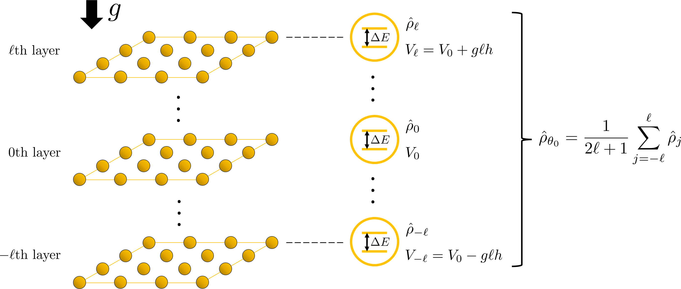
This section presents the calculation of the estimation accuracy of the gravitational potential when an $N_{\mathrm{layer}}$-layer optical lattice clock is used to estimate the gravitational potential. Specifically, after calculating the SLD Fisher information of the atomic clock, which is indistinguishable from each of the $N_{\mathrm{layer}}$-layers vertically aligned, we apply the quantum Cramér–Rao bound, assuming that there are $N_{\mathrm{site}}$ sets, to evaluate the variance of the estimated gravitational potential (see Fig. 3). This setup is based on the assumption that the observer can only perform measurements on single atoms and cannot distinguish the atoms being measured. The effective density operator of the entire system can then be written as the ensemble average of the density operators of the atomic clocks. Upon further assuming that each layer has the same population of atoms, the single-atom density operator can be obtained as

where $\rho_{j}$ is the density operator of an atom in the $j$th layer, $j$ is the label of a layers running from $-\ell$ to $\ell$, and $\theta_{0}\equiv 1+V_{0}/c^{2}$. Here, $N_{\mathrm{layer}}=2\ell+1$ denotes the total number of layers. The density operator in Eq. (15) can be derived as follows. Suppose that the observer performs the measurement corresponding to the single-atom POVM $(\hat{E}(x))$ but does not distinguish which atom is measured. The probability of obtaining outcome $x$ when the state is $\hat{\rho}_{j}$ is

Because each $\hat{\rho}_{j}$ is measured with an equal probability $1/N_{\mathrm{layer}},$ the probability of obtaining $x$ is given by

Noting that the POVM $\hat{E}$ is arbitrary, we conclude that the system state is effectively described by $\hat{\rho}_{\theta_{0}}$.

We assume that the gravitational field is uniform, gravitational acceleration is $g$, distance between layers is $h$, and gravitational potential in the $0$th layer is $V_{0}$. Then, on the basis of Eq. (6), the gravitational potential and the Hamiltonian of the atomic clock in the $j$th layer can be written as

and

where $\alpha\equiv\frac{gh}{c^{2}}$. If the initial state of each atomic clock is selected to be the superposition state $\frac{1}{\sqrt{2}}\left(\ket{0}+\ket{1}\right)$, the density operator $\hat{\rho}_{j}$ after time $\tau$ is given by

Therefore, on the basis of Eq. (15), we have

where $A\equiv\frac{\Delta E\tau}{\hbar}$. Then, Eq. (21) can be diagonalized as

Next, we evaluate the SLD Fisher information with respect to the parameter $\theta_{0}$. The SLD in this case is given by

Therefore, the SLD Fisher information is as follows:

Thus, if the variance of an estimator $\theta^{\mathrm{est}}$ of $\theta_{0}$ is expressed as $\mathrm{Var}\left[\theta_{0}^{\mathrm{est}}\right]$ and the number of atomic clocks in the same layer is $N_{\mathrm{site}}$, the quantum Cramér–Rao bound gives

By putting $A\equiv{\Delta E\tau}/{\hbar}$, $\theta_{0}\equiv 1+{V_{N}(x)}/{c^{2}}$, and $\alpha\equiv{gh}/{c^{2}}$, we obtain

The lower bound of ${\mathrm{Var}\left[V_{0}^{\mathrm{est}}\right]N_{\mathrm{site}}}/{c^{4}}$ in Eq. (27) is plotted as a function of ${\Delta E\tau}/{\hbar}$ in Fig. 4.

The implications of the lower bounds calculated as described in Secs. III and IV are discussed in this section. First, upon comparing Eqs. (13) and (27), the effect of gravitational dephasing is indicated by the factor $\left((2\ell+1){\sin\left[\frac{\Delta Egh}{2\hbar c^{2}}\tau\right]}/{\sin\left[\frac{\Delta Egh}{2\hbar c^{2}}(2\ell+1)\tau\right]}\right)^{2}$. Because of this factor, the lower bound of $\mathrm{Var}\left[V_{0}^{\mathrm{est}}\right]$, and hence $\mathrm{Var}\left[V_{0}^{\mathrm{est}}\right]$ itself, diverges at time

for integer $k$ unless ${k}/({2\ell+1})$ is an integer. This divergence is due to the progression of dephasing in the entire system, which is caused by an increase in the phase difference between the atomic clocks in each layer. The density operator of the system at time $\tau_{\mathrm{div}}$ is

and is in a completely mixed state. The recovery is due to further time evolution after divergence, which produces a layer wherein the phase difference is one lap behind. This resulted in a timing in which the phase coincides with the other layers.

As indicated by Fig. 4, the lower bound of $\mathrm{Var}\left[V_{0}^{\mathrm{est}}\right]$ has local minimum points owing to the balance between gravitational dephasing and accuracy improvement over time; the latter improvement is shown in the single-layer scenario in Sec. III. The point at which $\tau$ is the smallest among these local minimum points provides the principal limit of estimation accuracy when attempting to avoid divergence within a short period. To find the local minimum in an analytic manner, the following approximation is applied: When $2\ell+1\gg 1$ and $\tau$ are within the range $0<\tau<\frac{1}{2\ell+1}\frac{2\hbar c^{2}}{\Delta Egh}\pi$, we may approximate as $\sin\left[{\Delta Egh\tau}/({2\hbar c^{2}})\right]\backsimeq{\Delta Egh\tau}/({2\hbar c^{2}})$; hence,

Eq. (30) yields a local minimum value in the range $\tau>0$ at

and the lower bound of $\mathrm{Var}\left[V_{0}^{\mathrm{est}}\right]/c^{4}$ at $\tau_{\mathrm{min}}$ is

Therefore, when the number of layers in the optical lattice clock is sufficiently large, the lower bound of standard deviation in principle, while seeking to avoid divergence, is $\frac{1}{\sqrt{N_{\mathrm{site}}}}\frac{g(2\ell+1)h}{2c^{2}}$. This can be interpreted from two perspectives. First, it must be noted that $(2\ell+1)h$ is the height of the optical lattice clock. In this case, $g(2\ell+1)h$ is the gravitational potential difference $\Delta V$ between the top and bottom of the optical lattice clock. Eq. (32) implies that

where $\sigma(\cdot)$ denotes standard deviation. The RHS of Eq. (33) does not depend on the optical lattice clock details. Second, it must be noted that $2\ell+1$ is the number of layers of the optical lattice clock, $N_{\mathrm{layer}}$. In this case, the standard deviation is

If the atoms are equally spaced horizontally and vertically, ${N_{\mathrm{layer}}}/{\sqrt{N_{\mathrm{site}}}}$ can be regarded as the aspect ratio of the optical lattice clock. In particular, if the optical lattice clock has a shape with vertical and horizontal symmetry, such as a cube, we have ${N_{\mathrm{layer}}}/{\sqrt{N_{\mathrm{site}}}}=1$; therefore, the standard deviation depends only on the interlayer distance $h$.

The estimation accuracy begins to deteriorate when the interrogation time exceeds the time $\tau_{\mathrm{min}}=\frac{1}{2\ell+1}\frac{\hbar c^{2}}{\Delta Egh}\pi$. We now evaluate the specific value of $\tau_{\mathrm{min}}$ assuming a three-dimensional optical lattice clock. First, we calculate for Cd atoms. Because the wavelength is used as a clock for the Cd atoms, $\lambda^{\mathrm{Cd}}_{\mathrm{clock}}=$332\text{\,}\mathrm{nm}$$ Yamaguchi et al. 2019, $\Delta E=$6.0\text{\times}{10}^{-19}\text{\,}\mathrm{J}$$. In the optical lattice clock, atoms are captured in the antinode of the standing wave created by the electromagnetic wave of the corresponding magic wavelength; therefore, the spacing between each layer is approximately the magic wavelength of cadmium $\lambda^{\mathrm{Cd}}_{\mathrm{magic}}=$420\text{\,}\mathrm{nm}$$ Yamaguchi et al. 2019 and $h=$4.2\text{\times}{10}^{-7}\text{\,}\mathrm{m}$$. Assuming that the number of atoms that can be captured in a cubic optical lattice is 1 million, the number of atoms per side is 100, and $2\ell+1=100$. In this case, $\tau_{\mathrm{min}}$ is calculated as

This duration is approximately 33 hours. Similarly, we calculated $\tau_{\mathrm{min}}$ for other atoms (see TABLE 1). The values are roughly the same for all atoms, including Cd.

We evaluated the lower bounds of the variance of the estimators of the gravitational potential using optical lattice clocks based on the quantum Cramér–Rao bound. We then compared the results for the single-layer and multilayer optical lattice clocks. The results indicate that the lower bound of variance of the estimator using finite-size optical lattice clocks approaches zero with time in the single-layer scenario, whereas it diverges and recovers repeatedly owing to the effect of gravitational dephasing in the multilayer scenario. This effect also produces a local minimum point, indicating that there is a limit to the estimation accuracy because of the effect of gravitational dephasing when attempting to avoid the divergence of the lower bound. When the number of layers in the optical lattice clock is sufficiently large, the standard deviation of the estimate cannot be less than $\frac{N_{\mathrm{layer}}}{\sqrt{N_{\mathrm{site}}}}\frac{gh}{2}$. The interrogation time $\tau_{\mathrm{min}}$ required to reach this limit is determined to be $\frac{1}{2\ell+1}\frac{\hbar c^{2}}{\Delta Egh}\pi$. This standard deviation is independent of the optical lattice clock details. When $N_{\mathrm{layer}}$ and $\sqrt{N_{\mathrm{site}}}$ are comparable, the standard deviation is approximately equal to the distance between the layers of the optical lattice clock. The time $\tau_{\mathrm{min}}$ is calculated to be approximately 33 hours for a three-dimensional optical lattice clock consisting of one million Cd atoms on the Earth; the values are similar for other atoms.

In conclusion, there is certainly a limit to the lower bound of the variance of the estimators of the gravitational potential (i.e., the accuracy of gravitational potential estimation) using finite-size optical lattice clocks owing to gravitational dephasing. The lower bound is $\frac{N_{\mathrm{layer}}}{\sqrt{N_{\mathrm{site}}}}\frac{gh}{2}$ in standard deviation. Although this is applicable to general optical lattice clocks, it is extremely challenging to observe this limit, at least with current technology. This is because $\tau_{\mathrm{min}}$ is much larger than the current coherence time ($26\text{\,}\mathrm{s}$) as previously reported Zheng et al. 2022.

References

- Takamoto et al. (2020) M. Takamoto, I. Ushijima, N. Ohmae, T. Yahagi, K. Kokado, H. Shinkai, and H. Katori, Test of general relativity by a pair of transportable optical lattice clocks, Nat. Photonics 14, 411 (2020).
- Tanaka and Katori (2021) Y. Tanaka and H. Katori, Exploring potential applications of optical lattice clocks in a plate subduction zone, J. Geod. 95, 93 (2021).
- Zheng et al. (2022) X. Zheng, J. Dolde, V. Lochab, B. N. Merriman, H. Li, and S. Kolkowitz, Differential clock comparisons with a multiplexed optical lattice clock, Nature 602, 425 (2022).
- Bothwell et al. (2022) T. Bothwell, C. J. Kennedy, A. Aeppli, D. Kedar, J. M. Robinson, E. Oelker, A. Staron, and J. Ye, Resolving the gravitational redshift across a millimetre-scale atomic sample, Nature 602, 420 (2022).
- Pedrozo-Peñafiel et al. (2020) E. Pedrozo-Peñafiel, S. Colombo, C. Shu, A. F. Adiyatullin, Z. Li, E. Mendez, B. Braverman, A. Kawasaki, D. Akamatsu, Y. Xiao, and V. Vuletić, Entanglement on an optical atomic-clock transition, Nature 588, 414 (2020).
- Kawasaki (2022) A. Kawasaki, Decoherence of atomic ensembles in optical lattice clocks by gravity, J. Phys. Soc. Jpn. 91, 034301 (2022).
- Pikovski et al. (2015) I. Pikovski, M. Zych, F. Costa, and Č. Brukner, Universal decoherence due to gravitational time dilation, Nat. Phys. 11, 668 (2015).
- Ruiz et al. (2017) E. C. Ruiz, F. Giacomini, and Č. Brukner, Entanglement of quantum clocks through gravity, Proc. Natl. Acad. Sci. U.S.A. 114, E2303 (2017).
- Cepollaro et al. (2023) C. Cepollaro, F. Giacomini, and M. G. Paris, Gravitational time dilation as a resource in quantum sensing, Quantum 7, 946 (2023).
- Yamaguchi et al. (2019) A. Yamaguchi, M. S. Safronova, K. Gibble, and H. Katori, Narrow-line cooling and determination of the magic wavelength of cd, Phys. Rev. Lett. 123, 113201 (2019).
- Ludlow et al. (2008) A. D. Ludlow, T. Zelevinsky, G. K. Campbell, S. Blatt, M. M. Boyd, M. H. G. de Miranda, M. J. Martin, J. W. Thomsen, S. M. Foreman, J. Ye, T. M. Fortier, J. E. Stalnaker, S. A. Diddams, Y. L. Coq, Z. W. Barber, N. Poli, N. D. Lemke, K. M. Beck, and C. W. Oates, Sr lattice clock at fractional uncertainty by remote optical evaluation with a ca clock, Science 319, 1805 (2008).
- Barber et al. (2008) Z. W. Barber, J. E. Stalnaker, N. D. Lemke, N. Poli, C. W. Oates, T. M. Fortier, S. A. Diddams, L. Hollberg, C. W. Hoyt, A. V. Taichenachev, and V. I. Yudin, Optical lattice induced light shifts in an yb atomic clock, Phys. Rev. Lett. 100, 103002 (2008).
- McFerran et al. (2012) J. J. McFerran, L. Yi, S. Mejri, S. Di Manno, W. Zhang, J. Guéna, Y. Le Coq, and S. Bize, Neutral atom frequency reference in the deep ultraviolet with , Phys. Rev. Lett. 108, 183004 (2012).
- Kulosa et al. (2015) A. P. Kulosa, D. Fim, K. H. Zipfel, S. Rühmann, S. Sauer, N. Jha, K. Gibble, W. Ertmer, E. M. Rasel, M. S. Safronova, U. I. Safronova, and S. G. Porsev, Towards a mg lattice clock: Observation of the transition and determination of the magic wavelength, Phys. Rev. Lett. 115, 240801 (2015).
- Shao (2003) J. Shao, Mathematical statistics, 2nd ed., Springer texts in statistics (Springer, 2003).
- Petz and Ghinea (2011) D. Petz and C. Ghinea, Introduction to quantum Fisher information, in Quantum Probability and Related Topics (World Scientific, 2011).
- Helstrom (1976) C. W. Helstrom, Quantum detection and estimation theory, Mathematics in science and engineering : a series of monographs and textbooks No. 123 (Academic Press, 1976).
- Holevo (2011) A. S. Holevo, Probabilistic and statistical aspects of quantum theory, Quaderni monographs No. 1 (Edizioni della Normale, 2011).
- Watanabe (2014) Y. Watanabe, in Formulation of Uncertainty Relation Between Error and Disturbance in Quantum Measurement by Using Quantum Estimation Theory (Springer Tokyo, 2014) Chap. 4, pp. 37–44, 1st ed.
- Petz (1996) D. Petz, Monotone metrics on matrix spaces, Linear Algebra and its Applications 244, 81 (1996).