Passivity-based economic ports for optimal operation of networked DC microgrids

A schematic representation of a node composed of DGU and nonlinear load is shown in Figure 1. It consists of a Buck converter supplying a voltage $v_{\text{t},i}\in\mathbb{R}_{\geq 0}$, a nonlinear load with current $i_{{\text{L},i}}(v_{i})\in\mathbb{R}$, and a filter with inductance $L_{{\text{f},i}}\in\mathbb{R}_{>0}$, capacitance $C_{{\text{f},i}}\in\mathbb{R}_{>0}$, and resistance $R_{\text{f},i}\in\mathbb{R}_{>0}$. The Buck converter and the filter form a DGU. Each bus $i\in\mathcal{B}$ has two states, the node voltage $v_{i}$ and the filter current $i_{\text{f},i}$. The Buck converter voltage $v_{\text{t},i}$ is defined as the system input. Here, we use the well known averaging model for the Buck converter, by which we disregard the switching behavior [13]. The dynamics for every bus $i\in\mathcal{B}_{\text{DGU}}$ are [1, 14]

where $i_{\text{ext},i}$ is the cumulative current injected by interconnecting lines. The load is modeled with a voltage-dependent current source

where $y_{i}\in\mathbb{R}_{\geq 0}$ is the admittance of a constant resistive load, $p_{i}\in\mathbb{R}$ is a constant power load, and $\hat{i}_{\text{L},i}\in\mathbb{R}$ is a constant current load. Thus, the load is a linear combination of a constant resistive, a constant power and constant current load, which is also known as a nonlinear ZIP load [15].

The DGU described in Section II-A is normally equipped with a grid-forming or a grid-following controller [16]. Grid-forming controllers inject the necessary filter current $i_{{\text{f},i}}$ (indirectly power) in order to regulate the node voltage $v_{i}$ to a desired voltage reference $v_{\text{ref}}$, and stabilize thus the grid-voltages regardless of the load disturbance or volatile power injections. Grid-following controllers set the voltage $v_{\text{t},i}$ such that a given power reference $p_{\text{ref}}$ (indirectly the filter current $i_{{\text{f},i}}$) is injected, without considering the resulting node voltage level $v_{i}$. Grid-forming DGUs are used to achieve robust voltage stability, and grid-following DGUs to inject a certain amount of power irrespective of grid stability, e.g. for achieving optimal dispatch. Therefore, in this work, we have exactly one grid-forming DGU in every microgrid, and an arbitrary number of grid-following DGUs. The first DGU $1\in\mathcal{B}_{\text{DGU}}$ is defined without loss of generalization as the grid-forming DGU, while ${i\in\mathcal{B}_{\text{DGU}}\setminus\{1\}}$ are grid-following DGUs.

The grid-forming controller is taken from [1] and is designed by introducing an error state (3b) and a state feedback as

where $k_{\alpha,1}\in\mathbb{R}$, $k_{\beta,1}\in\mathbb{R}$ and $k_{\gamma,1}\in\mathbb{R}$ are the controller parameters. Similarly, the grid-following controller is designed here as

for all $i\in\mathcal{B}_{\text{dgu}}\setminus\{1\}$, using the injected power error (4b) instead. Note that the grid-following DGU introduces a nonlinearity when computing the injected power $v_{i}i_{{\text{f},i}}$ in (4b). Applying either (3) or (4) to the DGU (1) thus yields

depending if it is a grid-forming or grid-following DGU, with the variables $\alpha_{i}=\frac{k_{\alpha,i}-1}{L_{{\text{f},i}}}$, $\beta_{i}=\frac{k_{\beta,i}-R_{{\text{f},i}}}{L_{{\text{f},i}}}$ and $\gamma_{i}=\frac{k_{\gamma,i}}{L_{{\text{f},i}}}$ containing the controller parameters.

A load node is modeled as a DGU node without the filter and Buck converter. The dynamics are governed by the nonlinear dynamic equation

where $i_{{\text{L},i}}(v_{i})$ is the load as in (2).

The power lines $j\in\mathcal{E}$ interconnecting buses $i,h\in\mathcal{B}$ are modeled with the $\pi$-equivalent circuit [17], as shown in Fig. 2. It is composed of a series inductance $L_{{\pi,j}}\in\mathbb{R}_{>0}$ and resistance $R_{{\pi,j}}\in\mathbb{R}_{>0}$, and two parallel capacitances $\frac{C_{{\pi,j}}}{2}\in\mathbb{R}_{>0}$.

Note that the line capacitance is connected in parallel to the bus filter capacitance of the bus $i$ or $h\in\mathcal{B}$. Thus, the line capacitances are added to the DGU filter capacitances. The line dynamics are thus described by

where $v_{\Delta,j}=v_{i}-v_{h}$ is the input and $v_{i}$, $v_{j}$ are the bus voltages.

The whole microgrid is composed of $n=|\mathcal{B}|$ electrical buses with $d=|\mathcal{B}_{\text{DGU}}|\geq 1$ DGUs, interconnected by $m=|\mathcal{E}|$ power lines according to the graph $\mathcal{G}(\mathcal{B},\mathcal{E})$ with incidence matrix $M\in\mathbb{R}^{n\times m}$. With respect to the $d$ DGUs, recall that there is one grid-forming DGU which stabilizes the grid voltages and $d-1$ grid-following DGUs that inject power according to an economic objective function, which will be specified in Section III. The microgrid model reads

where $\alpha=[\alpha_{i}]$, $\beta=[\beta_{i}]$ and $\gamma=[\gamma_{i}]$ contain the control parameters, $C_{\text{f}}=[C_{{\text{f},i}}]$, $R_{\text{f}}=[R_{{\text{f},i}}]$, $L_{\text{f}}=[L_{{\text{f},i}}]$, $i_{{\text{L}}}=[i_{{\text{L},i}}]$, $R_{\pi}=[R_{{\pi,j}}]$ and $L_{\pi}=[L_{{\pi,j}}]$ are the filter, load and line parameters, and $v=\text{col}\{v_{i}\}\in\mathbb{R}^{n}$, $i_{\text{f}}=\text{col}\{i_{{\text{f},i}}\}\in\mathbb{R}^{d}$, $e=\text{col}\{e_{i}\}\in\mathbb{R}^{d}$ and $i_{\pi}=\text{col}\{i_{\pi,j}\}$ are the stacked states of the DGUs $i\in\mathcal{B}$ and power lines $j\in\mathcal{E}$. The voltage and power references $v_{\text{ref}}\in\mathbb{R}_{>0}$ and $p_{\text{ref}}\in\mathbb{R}^{d-1}$ are inputs, where $d$ defines the number of inputs of the microgrid. The matrix $I_{\text{f}}\in\mathbb{R}^{n\times d}$ is a permutation matrix assigning the filter currents of $d$ DGUs to the correct $n\geq d$ nodes. The matrices $I_{v}=\text{diag}\{1,0,\dots,0\}\in\mathbb{R}^{d\times d}$ and $I_{p}=\text{diag}\{0,1,\dots,1\}\in\mathbb{R}^{d\times d}$ are diagonal matrices such that the correct error signals are induced for the integrator states¹¹ 1 It holds that $I_{v}+I_{p}=I$, since all DGUs are either grid-forming or grid-following. as in (3b) and (4b). Note that in (8a) and (8d) it has been taken into account that the voltage drop over the power lines $v_{\Delta}$ can be expressed as $v_{\Delta}=M^{\top}v$ and the current drawn from the buses by the power lines as $i_{\text{ext}}=Mi_{\pi}$. The output $y$ of the system is defined as the filter current of the grid-forming DGU, which is set as the first filter current without loss of generality, i.e. $y=i_{{\text{f},1}}$.

In the next section, a price-based controller is designed in order to determine $p_{\text{ref}}$ such that an optimal steady state is achieved.

Inspired by the Linear-Convex Optimal Steady-State Control [18], we introduce an optimality model, which describes an optimal steady state where property (i) is fulfilled:

The function $f_{i}:\mathbb{R}\rightarrow\mathbb{R}$ represents the cost of the power infeed of the respective grid-following DGUs, which is assumed to be convex and quadratic in the paper at hand, i.e. $f(p_{\text{ref},i})=q_{i}p_{\text{ref},i}^{2}+r_{i}p_{\text{ref},i}+s_{i}$ with $q_{i},r_{i},s_{i}\in\mathbb{R}$, $q_{i}>0$. The variable $p_{\text{L}}$ comprises the sum of the power consumed by all loads and the losses of the microgrid. Thus, (9b) ensures power balance. The KKT conditions [19] for (9) are

where $\lambda\in\mathbb{R}$ is the Lagrange multiplier for the constraint (9b), and using a primal-dual gradient method [20, 21] with positive tuning parameters $\tau_{i}$ and $\kappa$, we get

The multiplier $\lambda$ can be interpreted as the electrical power price; if the load $p_{\text{L}}$ is greater than the power supplied by the grid-following DGUs, the price in (11b) increases and vice-versa. Equation (11a) means that the grid-following DGUs inject power such that their marginal costs equal the power price. This is the best solution for rational decision-makers, since feeding in more power would lead to less economic benefit per kW.

With controller (11), property (i) is fulfilled, since at steady state, every grid-following DGU produces at marginal cost and the grid-forming DGUs inject no power. However, property (ii) requires more attention. Even if (11a) can be computed by every grid-following DGU in distributed manner, the price-forming (11b) uses the load $p_{\text{L}}$ and the sum of the power injection $p_{\text{ref},i}$ of the grid-following DGUs, both being system-wide knowledge. To circumvent that, we present the following proposition.

In this subsection, we study the stability of the microgrid (8) controlled with (17). Define the state variable $x=\text{col}\{v,i_{\text{f}},e,i_{\pi},p_{\text{ref}},\lambda\}\in\mathbb{R}^{n_{\text{cl}}}$ with $n_{\text{cl}}=n+3d+m$ the number of states, and let $\bar{x}$ be an equilibrium point of the closed-loop system for a constant $v_{\text{ref}}$. In shifted coordinates $\tilde{x}=x-\bar{x}$, the nonlinear closed-loop system reads

with

where $v=\bar{v}+\tilde{v}$, $i_{\text{f}}=\bar{i}_{\text{f}}+\tilde{i}_{\text{f}}$, $Q=[\tau_{i}q_{i}]$, $\tau=\text{col}\{\tau_{i}\}$ and $Y=[y_{i}]$. The constant power load $P=\text{col}\{p_{i}\}\in\mathbb{R}^{n}$ is seen as a variable here, since we consider it to vary over time.

In the following, we present a condition to assess stability of the closed-loop system by solving a semi-definite program.

The following electric port defines an interface for interconnecting microgrids via electric lines.

The electric port is interfaced with system (18) through the vectors $b_{\text{elec}}^{k}=\text{col}\{t_{i},0_{3d+m}\}$ and $c_{\text{elec}}^{k}=b_{\text{elec}}^{k\top}$, where $t_{i}\in\mathbb{R}^{n}$ has a 1 at the $i$-th element and zero elsewhere, since an external current drawn to a node $i\in\mathcal{B}$ acts on the voltage dynamics (1a) or (6) of node $i\in\mathcal{B}$. Note that a microgrid may contain an arbitrary number $z\in\mathbb{R}$ of electric ports, yielding matrices $B_{\text{elec}}^{k}=[b_{\text{elec},1}^{k},\dots,b_{\text{elec},z}^{k}]$ and $C_{\text{elec}}^{k}=B_{\text{elec}}^{k\top}$.

The following economic port defines an interface for interconnecting microgrids economically.

When the economic port $(\lambda_{\text{ext}}^{k},\lambda_{\text{loc}}^{k})$ is connected, we replace the price used for the grid-following DGUs in (17a) with the input $\lambda_{\text{ext}}^{k}$, yielding

The local price $\lambda_{\text{loc}}^{k}$ (output of economic port) is still determined by the current of the grid-forming DGU, but is no longer used directly in the local microgrid. Splitting the price in a microgrid into local and external prices allows, using a special interconnection structure for economic ports as proposed in Section IV-B, the local price $\lambda_{\text{loc}}^{k}$ to contribute towards a (global) external price. The external price then already implicitly contains a coordination between microgrids, and is used by the grid-following DGUs in order to achieve global optimal dispatch. Note that only a single economic port per microgrid is allowed in this work, since we have a single local price per microgrid.

The economic port thus interfaces with the system (18) through the vectors $b_{\text{econ}}^{k}=\text{col}\{0_{n+2d+m},\tau,0\}$ and $c_{\text{econ}}^{k}=\text{col}\{0_{n+3d+m-1},1\}$. System (18) with electric and economic ports reads then

The matrix $A_{\lambda}^{k}(\cdot)$ is the same as $A(\cdot)$ in (18) except that (24a) replaces (17a), where the input $\lambda_{\text{ext}}^{k}$ is used instead of the state from (24b). Vector $i_{\text{elec}}^{k}=\text{col}\{i_{\text{elec},z}^{k}\}$ is the input for all electric ports $z$.

We are now interested in the dissipativity properties of the interconnection ports, in order to analyse microgrids interconnected via physical-electric or information-economic ports. First, we analyse the dissipativity properties of the electric port; thereafter, the properties of the economic port.

The interconnection of microgrids with electric ports through electric lines is analogous to the interconnection of nodes via electric lines as explained in Section II. Given a connected interconnection topology, the interconnection of nodes via electric lines constitutes a skew-symmetric interconnection as shown in [1]. Thus, microgrids with electric ports fulfilling Proposition 3 or Theorem 1 interconnected via electric lines are guaranteed to be asymptotically stable.

We now consider a set $\mathcal{M}$ of microgrids interconnected electrically and economically, using the port properties established in Theorem 1. To this end, we first characterize a globally optimal steady state for economically interconnected microgrids.

We consider a meshed DC microgrid with 8 nodes and 9 lines interconnected via electric lines (purple) to a second meshed DC microgrid with 4 nodes and 4 lines shown in Figure 3, which was adapted from the scenario in [12]. In Microgrid 1, Node 4 (turquoise) is equipped with a grid-forming DGU, which stabilizes the grid dynamics and acts here as price-forming entity. Nodes 2, 3 and 4 (red) have a grid-following DGU, which are the price-taking feeders. The cost of the power injection is set to $f_{1}^{1}(p_{1})=1.2p_{1}^{2}$, $f_{2}^{1}(p_{2})=1.3p_{2}^{2}$ and $f_{3}^{1}(p_{3})=1.4p_{3}^{2}$. All other nodes (black) consist only of nonlinear loads (2). In Microgrid 2, the grid-forming DGU is located at Node 3. Grid-following DGUs are located at Node 1 and 4, while Nodes 2 consists only of a nonlinear load. The cost of the power injection is set for the DGUs in microgrid 2 to $f_{1}^{2}(p_{1})=1.4p_{1}^{2}$ and $f_{4}^{2}(p_{4})=1.5p_{4}^{2}$.

Load steps occur at time $t_{1}=$20\text{\,}\mathrm{s}$$ and $t_{2}=$40\text{\,}\mathrm{s}$$. The total load of the microgrids after the load steps is shown in Table I. At $t_{1}=$20\text{\,}\mathrm{s}$$, we have only an increase of the load in Microgrid 1 and hence an increase in the sum of the loads in both microgrids. At $t_{2}=$40\text{\,}\mathrm{s}$$, the load in Microgrid 1 decreases but increases in Microgrid 2, such that the sum of the loads decreases.

The reference voltage $v_{\text{ref}}$ is set to $1000\text{\,}\mathrm{V}$. Typical parameter values for the lines and DGU parameters are taken from [14].

In the next section, two microgrids interconnected through electric ports are considered in order to highlight the plug-and-play stability of microgrids stated in Proposition 3.

In this section, the microgrids interconnected via the electric lines (purple) as shown in Figure 3 are considered. For both microgrids, Proposition 3 is verified for the subset of the state space defined via $v_{\min}=$950\text{\,}\mathrm{V}$$, $v_{\max}=$1050\text{\,}\mathrm{V}$$ for all nodes and $i_{\text{f},\min}=$-15\text{\,}\mathrm{A}$$, $i_{\text{f},\max}=$15\text{\,}\mathrm{A}$$ for all filter currents.

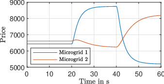
The power injection of the grid-following DGUs and the price in both microgrids are shown in Figures 4 and 5, respectively. When the load step at $t_{1}=$20\text{\,}\mathrm{s}$$ occurs, the DGUs in Microgrid 1 increase their power injection, while the DGUs in Microgrid 2 decrease their power injection, even if the sum of the loads increased (see Table I). At $t_{2}=$40\text{\,}\mathrm{s}$$, the power injection in Microgrid 1 decreases and increases in Microgrid 2, following the trend of their own load (see Table I).

Similar dynamics are also shown by the price in Figure 5. In particular, the price dynamics in both microgrids depend on the local microgrid load changes rather than on the sum of the loads across all microgrids. The microgrids are thus not cooperating, since the economic ports are not considered. As can be observed, the prices in both microgrids are not equal at any steady-state, which entails suboptimal economic dispatch. Furthermore, the steady-state prices cannot be directly influenced, since it results from the grid-forming controllers in each microgrid, which may not have identical parameters.

In order to influence the prices in each microgrid and obtain global economic optimal dispatch, an interconnection via the economic ports as described in Section IV-B is employed in the next subsection.

In this subsection, the networked microgrids are equipped with the economic ports and the dynamic averaging as in Section IV-B. Theorem 1 is verified for the same subset of the state space as in Section V-B.

The power injection of the grid-forming DGUs and the price in both microgrids are shown in Figures 6 and 7, respectively. When a load step occurs, the prices in both microgrids vary. However, after a transient period, the prices in both microgrids are equal. This is due to the consensus algorithm (29) interconnecting the microgrids via the economic port, which achieves a price consensus at steady state. The power injections of the grid-following DGUs in Figure 6 adjusts automatically according to the price in the microgrids. Note that the DGUs of Microgrid 2 inject less power than the DGUs in Microgrid 1, since they have greater injected power costs (see Section V-A). DGUs with the same cost function (e.g. $f_{3}^{1}$ and $f_{4}^{2}$) inject the same amount of power in steady state despite being in different microgrids with different loads. Since at steady state a price consensus of both microgrids is achieved, we have optimal dispatch at steady state according to Proposition 4. Note that optimal dispatch is achieved solely by an exchange of the local prices in a distributed manner via the economic ports.

References

- [1] Pulkit Nahata, Raffaele Soloperto, Michele Tucci, Andrea Martinelli and Giancarlo Ferrari-Trecate “A passivity-based approach to voltage stabilization in DC microgrids with ZIP loads” In Automatica 113 Elsevier, 2020, pp. 108770
- [2] Felix Strehle, Martin Pfeifer, Albertus Malan, Stefan Krebs and Sören Hohmann “A Scalable Port-Hamiltonian Approach to Plug-and-Play Voltage Stabilization in DC Microgrids” In IEEE Conf. on Control Technology and Applicat., 2020
- [3] Jeremy Watson, Yemi Ojo, Ioannis Lestas and Chrysovalantis Spanias “Stability of power networks with grid-forming converters” In 2019 IEEE Milan PowerTech, 2019, pp. 1–6 DOI: 10.1109/PTC.2019.8810506
- [4] Pulkit Nahata, Mustafa Turan and Giancarlo Ferrari-Trecate “Consensus-Based Current Sharing and Voltage Balancing in DC Microgrids With Exponential Loads” In IEEE Trans. on Control Syst. Technol. 30.4, 2022, pp. 1668–1680 DOI: 10.1109/TCST.2021.3120321
- [5] Albertus Malan, Pol Jane-Soniera, Felix Strehle and S“”oren Hohmann “Passivity-based power sharing and voltage regulation in DC microgrids with unactuated buses” In arXiv preprint arXiv:2301.13533, 2023 URL: https://arxiv.org/abs/2301.13533
- [6] Yemi Ojo, Jeremy Watson, Khaled Laib and Ioannis Lestas “A Distributed Scheme for Voltage and Frequency Control and Power Sharing in Inverter-Based Microgrids” In IEEE Trans. on Control Syst. Technol. IEEE, 2023
- [7] Tjerk Stegink, Claudio De and Arjan van Schaft “A unifying energy-based approach to stability of power grids with market dynamics” In IEEE Trans. on Autom. Control 62.6 IEEE, 2016, pp. 2612–2622
- [8] Lukas K“”olsch, Katharina Wieninger, Stefan Krebs, a and S“”oren Hohmann “Distributed frequency and voltage control for ac microgrids based on primal-dual gradient dynamics” In IFAC-PapersOnLine 53.2 Elsevier, 2020, pp. 12229–12236
- [9] Pol Jan“’e-Soneira, Ionela Prodan, Albertus Malan and S“”oren Hohmann “On MPC-based Strategies for Optimal Voltage References in DC Microgrids” In 2023 European Control Conference (ECC), 2023, pp. 1–6 IEEE
- [10] Pol Soneira, Ionela Prodan and Soeren Hohmann “Optimal Voltage References for DC Microgrids using an Economic MPC Approach” In Book of abstracts PGMO DAYS 2022, 2022, pp. 67
- [11] Florian D“”orfler, John Simpson-Porco and Francesco Bullo “Breaking the hierarchy: Distributed control and economic optimality in microgrids” In IEEE Trans. on Control of Netw. Syst. 3.3 IEEE, 2015, pp. 241–253
- [12] Jinxin Zhao and Florian D“”orfler “Distributed control and optimization in DC microgrids” In Automatica 61 Elsevier, 2015, pp. 18–26
- [13] R.. Middlebrook and Slobodan Cuk “A general unified approach to modelling switching-converter power stages” In IEEE Power Electron. Specialists Conf., 1976, pp. 18–34 DOI: 10.1109/PESC.1976.7072895
- [14] Michele Tucci, Stefano Riverso, Juan. Vasquez, Josep. Guerrero and Giancarlo Ferrari-Trecate “A Decentralized Scalable Approach to Voltage Control of DC Islanded Microgrids” In IEEE Trans. on Control Syst. Technol. 24.6, 2016, pp. 1965–1979 DOI: 10.1109/TCST.2016.2525001
- [15] Prabha Kundur and Om Malik “Power system stability and control” McGraw-Hill Education, 2022
- [16] Joan Rocabert, Alvaro Luna, Frede Blaabjerg and Pedro Rodriguez “Control of power converters in AC microgrids” In IEEE Trans. on power electronics 27.11 IEEE, 2012, pp. 4734–4749
- [17] Jan Machowski, Zbigniew Lubosny, Janusz Bialek and James Bumby “Power system dynamics: stability and control” John Wiley & Sons, 2020
- [18] Liam Lawrence, John Simpson-Porco and Enrique Mallada “Linear-convex optimal steady-state control” In IEEE Trans. on Autom. Control 66.11 IEEE, 2020, pp. 5377–5384
- [19] Stephen Wright and Jorge Nocedal “Numerical optimization” In Springer Science 35.67-68, 1999, pp. 7
- [20] J Arrow, L Hurwicz, H Uzawa and H Chenery “Studies in Linear and Nonlinear Programming” Stanford University Press, 1958
- [21] Diego Feijer and Fernando Paganini “Stability of primal-dual gradient dynamics and applications to network optimization” In Automatica 46.12 Elsevier, 2010, pp. 1974–1981
- [22] Hassan Khalil “Nonlinear systems third edition” In Patience Hall 115, 2002
- [23] Stephen Boyd, Laurent El, Eric Feron and Venkataramanan Balakrishnan “Linear matrix inequalities in system and control theory” SIAM, 1994
- [24] George Hines, Murat Arcak and Andrew Packard “Equilibrium-independent passivity: A new definition and numerical certification” In Automatica 47.9 Elsevier, 2011, pp. 1949–1956
- [25] Rodolphe Sepulchre, Mrdjan Jankovic and Petar Kokotovic “Constructive nonlinear control” Springer Science & Business Media, 2012
- [26] Solmaz Kia, Bryan Van, Jorge Cortes, Randy Freeman, Kevin Lynch and Sonia Martinez “Tutorial on dynamic average consensus: The problem, its applications, and the algorithms” In IEEE Control Syst. Magazine 39.3 IEEE, 2019, pp. 40–72
- [27] Randy Freeman, Peng Yang and Kevin Lynch “Stability and convergence properties of dynamic average consensus estimators” In Proceedings of the 45th IEEE Conference on Decision and Control, 2006, pp. 338–343 IEEE
- [28] Arjan Van Schaft “L2-gain and passivity techniques in nonlinear control” Springer, 2017