Variance extrapolation method for neural-network variational Monte CarloPreprint: APS/123-QED
Abstract
Constructing more expressive ansatz has been a primary focus for quantum Monte Carlo, aimed at more accurate ab initio calculations. However, with more powerful ansatz, e.g. various recent developed models based on neural-network architectures, the training becomes more difficult and expensive, which may have a counterproductive effect on the accuracy of calculation. In this work, we propose to make use of the training data to perform variance extrapolation when using neural-network ansatz in variational Monte Carlo. We show that this approach can speed up the convergence and surpass the ansatz limitation to obtain an improved estimation of the energy. Moreover, variance extrapolation greatly enhances the error cancellation capability, resulting in significantly improved relative energy outcomes, which are the keys to chemistry and physics problems.
I Introduction
Recent decades have brought significant advances in simulating complicated physical systems using computers, making it possible to model and understand intricate phenomena with unprecedented accuracy and detail. Consequently, computer simulation is now considered the “third way” of doing science, bridging the gap between theory and experiment Foulkes et al. 2001. In the fields of physics and chemistry, a crucial problem lies in determining the electronic structure through solving the Schrödinger equation, a fundamental task in the realm of quantum mechanics Pople 1999; Kohn 1999. Although the underlying physical laws have been well-understood for almost a century, “the difficulty is only that the exact application of these laws leads to equations much too complicated to be soluble.”, as Paul Dirac famously wrote Dirac 1929. Solving the 3-dimensional Schrödinger equation describing a system containing interacting electrons seems impossible, but this is exactly what quantum Monte Carlo (QMC) methods allow us to do Foulkes et al. 2001.
QMC comprises of a wide range of stochastic methods based on random sampling Austin et al. 2012. One of the most frequently used methods is the variational Monte Carlo (VMC) McMillan 1965; Ceperley et al. 1977. The basic idea of VMC involves assuming a particular wavefunction ansatz and applying the variational principle to optimize it towards the ground state. Apparently, the accuracy of VMC is restricted by the expressiveness of the ansatz, which motivates the construction of more powerful ansatz. Recently, various neural-network-like wavefunction ansatz have been proposed and greatly improved the accuracy of VMC Carleo and Troyer 2017; Schütt et al. 2017; Gao and Duan 2017; Cai and Liu 2018; Cai and Liu 2018; Han et al. 2019; Luo and Clark 2019; Pfau and Foulkes 2020; Choo et al. 2020; Spencer et al. 2020; Hermann et al. 2020; von Glehn et al. 2022; Lin et al. 2023; Abrahamsen and Lin 2022; Gerard et al. 2022; Pescia et al. 2022; Wilson et al. 2023; Scherbela et al. 2022; Li et al. 2022; Gao and Günnemann 2021; Gao and Günnemann 2022; Gao and Günnemann 2023; Scherbela et al. 2023; Barrett et al. 2022; Zhao et al. 2023. For convenience, we refer to this as neural-network VMC (NN-VMC) in the following text. FermiNet Pfau and Foulkes 2020; Spencer et al. 2020 and DeepSolid Li et al. 2022 are examples of successful wavefunction ansatz for molecular and periodic systems respectively.
Despite the success of NN-VMC in accuracy, its widespread use is limited by the high computational cost incurred by the large number of parameters to be optimized and the long training process required for convergence. This results in the unsatisfactory error cancellation capability Ren et al. 2023, which is essential for estimating relative energy, such as ionization energy, dissociation energy and so on. Previously when calculating relative energies, identical hyperparameters were shared across different systems, and the discrepancies between total energy outcomes were regarded as the results. This strategy, however, is fair but unbalanced, since a relative energy involves the energies of two different systems, but a more complicated system may require a larger network to handle, and the speed of convergence can differ across different systems.
In this work, we propose to make use of the large amount of energy-versus-variance data obtained during the prolonged training process to perform zero variance extrapolation in NN-VMC. We evaluate this extrapolation approach across a range of systems, including N2 molecules of varying bond lengths and some well known periodic systems, using respectively FermiNet and DeepSolid as the wavefunction ansatz. We also incorporate the variance matching method for N2 molecules. Although the results of variance matching method appear to be unsatisfactory, our proposed extrapolation approach demonstrates high performance across all systems. Notably, the extrapolation is solely based on training data, without incurring additional computational costs. In addition to obtaining better relative energy, it can surpass the limitation of the wavefunction ansatz and mitigate the bias caused by the inadequate training convergence, thus also delivering an better evaluation of total energy, which is also discussed.
II Methods
II.1 VMC theory
VMC is a stochastic method for solving quantum many-body problems. For a complex quantum system, the many-body Hamiltonian operator can be expressed as
| (1) |
where are subscripts for electrons, and for nuclei. denotes the charges, and denote the positions. Under Born-Oppenheimer approximation Born and Oppenheimer 1927, the main goal is to obtain the ground state wavefunction and corresponding energy of the stationary Schrödinger equation,
| (2) |
To accomplish this, VMC employs Monte Carlo methods to handle the high dimensional energy integral and variational principles to optimize the wavefunction towards the ground state. Given a wavefunction ansatz , its energy expectation is defined as
| (3) |
where is the normalized wavefunction squared, i.e. the probability density function, and is the so-called local energy function. The outcome of this energy integral must be greater than the ground state energy, which is the target of VMC, so we just need to optimize the wavefunction towards lower energy,
| (4) |
Keep optimizing until convergence, and we will get the approximation of ground state wavefunction and corresponding energy, whose accuracy depends on the expressiveness of the wavefunction ansatz.
II.2 Better relative energy in NN-VMC
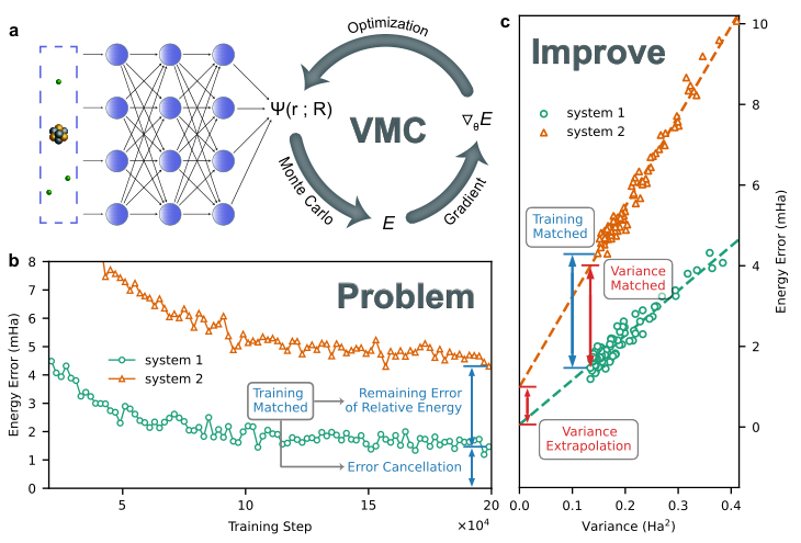
NN-VMC reaps the benefit of a vast number of parameters to obtain high accuracy. However, this comes at the cost of a lengthy optimization process, which unfortunately results in less satisfactory error cancellation capability when calculating the relative energy. Since there is no established criterion for measuring the degree of convergence during the training, the common approach is to use the same optimization iteration in all the systems for calculating relative energies, as shown in Fig. 1b and labeled as “Training Matched” (TM). Nevertheless, this can lead to an unbalanced treatment if the optimization is inadequate for convergence because of the different speed of convergence in different systems. Even if achieving complete convergence, this simple fairly-treating approach is still unbalanced as the more complicated system requires a larger network to obtain the same accuracy.
To achieve balanced treatments, matching a quantity related to the error in a wavefunction is a potential strategy, which has been utilized in various studies to obtain excitation energy Robinson et al. 2017; Pineda Flores and Neuscamman 2019; Otis et al. 2020; Garner and Neuscamman 2020; Entwistle et al. 2023. The energy variance is selected as the matching quantity and is defined as:
| (5) |
where denotes the energy expectation. As shown in Fig. 1c, the “Variance Matched” (VM) method is thus comparing the energies of two systems where they have the same variance. To clarify further, we choose the data point with the most training steps from “system 1” and compare its energy result with “system 2”, whose energy result is determined via linear regression at the corresponding variance.
Another strategy is the zero-variance extrapolation method, where the energy outcomes are extrapolated until the variance reaches zero as the real ground state should possess zero energy variance. In VMC, when the wavefunction is optimized to be near the ground state, the energy and variance exhibit a linear relationship, as demonstrated in Fig. 1c. Although the fundamental reason for the linear relationship is not fully clear Kwon et al. 1993; Kwon et al. 1998, it leads to empirical extrapolation schemes that have been successfully used in various systems, including Fermi liquids and the Hubbard model Taddei et al. 2015; Robledo Moreno et al. 2022; Hu et al. 2013; Iqbal et al. 2016. The most commonly used schemes for extrapolation in previous studies are: 1) based on the converged results of different ansatz, such as different forms of backflow or different widths of the network Taddei et al. 2015; Robledo Moreno et al. 2022, and 2) based on the results of different converged degrees with the same ansatz, such as different Lanczos steps Hu et al. 2013; Iqbal et al. 2016. In other words, there are two different routes to obtain a range of wavefunctions with different “distance” to the ground truth. In this work, we employ extrapolation based on the training data at different converged levels of NN-VMC, as shown in Fig. 1c, labeled as “Variance Extrapolation” (VE).
To obtain effective information from the noisy training data, a rolling window is employed to calculate the robust mean of the energy and variance, which means in each window the outlier data are masked. We assume that the wavefunction in a window does not change much, and the energy data follow the normal distribution. For a window containing data points, the data points whose absolute deviation of the energy from the median is larger than 3 are considered to be outliers, where is the standard deviation. In all the calculations we mentioned in this paper, we set the window size to be 2000. After masking, the energy and variance outcomes of this window are calculated following:
| (6) |
where and denote the energy and variance of the remaining data after masking, and the overline denotes taking the average. It is worth pointing out that in the training process of NN-VMC, there may be extreme outliers that can significantly impact the extrapolation outcome, thus making the masking step indispensable.
For more technical details about the selection of linear segments for extrapolation and the appropriateness of using training data rather than inference data, refer to Supplementary Note 1.
II.3 Linear relationship in VE method
In the VE method, we assume that there exists linear relationship between the energy and the energy variance when the wavefunction is nearing the ground state. As mentioned earlier, the fundamental reason for the linear relationship remains unclear. However, we can provide a possible explanation by offering a sufficient but unnecessary condition for such a relationship, following the idea of Kashima et al. Kashima and Imada 2001.
In the late training period, assume that the neural-network state can be represented as a linear combination of ground state component and another fixed eigenstate of Hamiltonian . That is,
| (7) |
Here , corresponding to the ground state’s dominance as the training process approaches convergence. Without loss of generality, here we assume the normalization condition . The energy expectation result is
| (8) |
where and are the eigenvalues, i.e. the energies corresponding to and . The energy variance result is
| (9) |
We can thus derive the linear relationship
| (10) |
where the slope factor .
III Results and Discussion
III.1 N2 molecule

We now discuss the tests of the VM and VE methods on N2 molecule in more detail. N2 molecule is strongly correlated at the breaking-bond region due to the complexity of triple-bond breaking, providing a challenge case for accurate wavefunction calculation. Energies at three bond lengths are calculated using FermiNet as the wavefunction ansatz, including Bohr at the equilibrium geometry, Bohr in the strongly correlated region and Bohr in the completely dissociated region. As shown in Fig. 2a, the energy and variance show linear relationship at all the three bond lengths, which makes it possible for VM and VE methods to be applied.
The energy differences relative to the equilibrium geometry and are investigated respectively using TM, VM and VE methods, as illustrated in Fig. 2b. Because of the high accuracy of FermiNet on the N2 molecule at bond lengths and , the TM method can already provide a good estimate of , leaving only a little room for improvements. Still and all, it is obvious that the VE method performs better than the VM method. Regarding , when the accuracy of FermiNet at decreases due to the strong correlation, the TM method becomes inadequate in providing a reliable result. In this case, the VM method can lead to only a minor improvement, whereas the VE method significantly reduces the error by 67.8%, from 2.84 mHa to 0.92 mHa.
In Fig. 2c, we further investigate the convergence and fluctuation patterns of and along the training process when using respectively TM, VM and VE method. The VE method’s curves begin at the training step of in order to ensure a sufficient number of data points for the linear regressions. Compared with the results obtained through the TM and VM methods, the VE method exhibits faster convergence and a much quicker reduction in fluctuation. By the th training step, the VE method has achieved convergence for both and , with smooth curves and no fluctuations. This suggests that using the VE method, VMC training does not require complete convergence, resulting in significant computational cost savings.
To further verify the reliability of the VE method, we tested it on the N2 dissociation curve, which contained calculations of N2 molecule at 25 different bond lengths, involving intact and breaking triple bond (Fig. 2d). For comparison, the state-of-the-art r12-MR-ACPF results Gdanitz 1998 are also displayed. Considering total energy, all the results show remarkable progress after variance extrapolation, and most results are refined to be within chemical accuracy. As for the non-parallelity error, i.e. the difference between the maximum and the minimum errors along the curve, the VE method enhances the original result of 4.53 mHa to 2.89 mHa, which is comparable to the r12-MR-ACPF result of 2.14 mHa. The corresponding extrapolation details are presented in Supplementary Fig. 2. Since it is a bit arbitrary to choose which of the 25 different bond lengths to match the energy variance, the VM method is not tested here.
Finally, it is worth noting that by improving the accuracy of total energy estimations, it becomes easier to accurately derive certain types of relative energy, such as dissociation energy. Normally, we have two strategies for calculating the dissociation energy of a system AB containing two parts A and B,
| (11) | ||||
| (12) |
where denotes the energy of the AB system, and denote the energies of the individual monomers A and B, and denotes the energy of the system consisting of separate monomers A and B at a sufficient distance from each other. If a difference appears in and , then it is often regarded as the appearance of size inconsistency of the calculation, which would cause severe problems when computing useful quantities such as the dissociation energy of molecules. In traditional wavefunction methods the size consistency problem is often induced by an limited ansatz, and in NN-VMC the unbalanced optimization of two different systems is also an important contribution of the problem. Curing the relative energy error is effectively improving the size consistency property of NN-VMC calculations.
In Fig. 2b, and are the dissociation energies of the N2 molecule respectively following Eq. 11 and Eq. 12, where denotes the energy of atom N reported by Chakravorty et al. Chakravorty et al. 1993. Apparently, both and would have upward biases due to the limit of ansatz expressiveness. Before the extrapolation, performs better than as the two biases cancel each other out to a large extent. Through extrapolation, we obtain an improved estimate of and thus greatly improve the accuracy of without the requirement of , which saves half the computational cost. Generally speaking, and are much simpler to obtain precise results than because of the computational complexity of at least in terms of the system size for accurate quantum Monte Carlo calculations. Therefore, the VE method providing better total energy results may help a lot on calculating dissociation energy.
To summarize, we show that the VE approach is an effective method for enhancing the accuracy of total energy and relative energy outcomes without incurring additional computational expenses. In contrast, it appears that the VM approach may not provide significant benefits for calculations at this level of accuracy.
III.2 Periodic Systems
Periodic systems are different from molecules, where the system is in principle infinitely large while molecules contain a finite number of atoms. Nevertheless, a similar problem would occur because of an improper wavefunction ansatz or unbalanced optimization. To compute the useful quantities for periodic systems, such as the cohesive energy of solids, it is required to maintain the size extensiveness of the calculation, otherwise the errors are too significant. To verify whether the VE method also works for periodic systems and improves the size extensiveness, we further analyze two other calculations on periodic systems reported in DeepSolid Li et al. 2022, namely the one-dimensional hydrogen chain and the two-dimensional graphene.
Hydrogen chain is a simple but challenging and interesting system. Fig. 3a shows the interaction energy results of different hydrogen chains containing different atom numbers in a supercell and the corresponding extrapolation result to the thermodynamic limit (TDL). The extrapolation simply follows the quadratic curve fitting with the symmetry axis fixed at 0. For comparison, the TDL auxiliary field quantum Monte Carlo (AFQMC) energy result at complete basis set (CBS) limit is also plotted Motta et al. 2017. Upon observing the magnified results depicted in the inset diagram, it is clear that the TDL energy result utilizing the VE method is more consistent with the AFQMC result. Returning to the four finite size results, the VE method has led to a downward correction on each of them. The larger the system, the bigger the VE method’s correction, which is both expected and reasonable given that the accuracy of DeepSolid may progressively worsen on larger systems. The corresponding extrapolation details are shown in Supplementary Fig. 3.
Graphene is a famous two-dimensional material attracting broad attention over last two decades Geim 2011. The real space and k-space structure of graphene are illustrated in Fig. 3b. The positions of three special k points sampled following Monkhorst-Pack mesh Monkhorst and Pack 1976; Pack and Monkhorst 1977 are also marked, at which the cohesive energy is calculated. The corrected result is regarded as the weighted average of the results at the three k points under twist-averaged boundary condition (TABC) plus an additional structure factor Li et al. 2022; Lin et al. 2001; Chiesa et al. 2006. Compared with the experimental result, it is obvious that the VE method enhances the result. The corresponding extrapolation details are displayed in Supplementary Fig. 4.
The homogeneous electron gas (HEG) system presented in DeepSolid Li et al. 2022 is also tested, and the corresponding results are shown in Fig. 4. In each panel, the correlation energies (i.e., enhancements from the Hatree-Fock method) calculated by various methods are plotted, and a upper bound of the exact result is marked using red dashed lines, which utilizes the variational property of the BF-DMC results Ríos et al. 2006. While the initial results prior to extrapolation fall above the upper bound, the results subsequent to extrapolation almost consistently surpass the upper bound. For the densities Bohr, where TC-FCIQMC results are available Liao et al. 2021, the red full lines indicate high-accuracy benchmarks. The extrapolation results at both densities are closer to the red full lines. The corresponding extrapolation details are displayed in Supplementary Fig. 5.
The success of the VE method on the periodic systems further illustrates its universality and reliability.
IV Discussion
Based on our experience, the VE method should be considered as icing on the cake rather than a universal energy correction scheme. The premise of this method is small enough energy variance, where the energy results are already very accurate. For example, in all the calculations we report in this work the energy variance converges to 0.5 Ha2 or less and the energy results are only several millihatrees from the exact results (see Supplementary Fig. 2–5). The VE method here is to take the last small step forward, from excellence to superexcellence. However, this small step in total energy may be a big step in relative energy, which makes it essential. Besides, the slope of energy versus variance linear regression can be a very useful analysis aspect when examining different systems. Having demonstrated the effectiveness of the VE method, it is worth noting that the applications of VE method to large systems would face two challenges and the method should be executed with care. Firstly, as far as our training can reach, the wavefunction is still far from ground state, and the energy variance remains large. Secondly, there is big energy fluctuation during the training process of such large systems, which decreases the data quality and affects the extrapolation results.
V Conclusion
In conclusion, we propose a new extrapolation technique based on the training data in NN-VMC, which appears to be an effective and efficient solution for a balanced treatment to obtain better error cancellation when calculating relative energies. Additionally, this method can surpass the limitation of the wavefunction ansatz and obtain an improved estimation of total energy, which is also important in some cases. Furthermore, employing the VE method yields quicker convergence of energy results with reduced fluctuations, leading to significant savings in computational costs. Since this approach has shown great power on both FermiNet and DeepSolid, encompassing both molecular and periodic systems, we expect that it will also greatly contribute to the future of NN-VMC on various powerful ansatz.
Acknowledgements.
The authors thank Xiang Li for sharing data and results. We thank Hang Li for support, Xuelan Wen for relevant literature research, and Liwei Wang, Di He, Chuwei Wang, Du Jiang, Ruichen Li and the rest of the teams for helpful discussions. J.C. is funded by the National Natural Science Foundation of China under Grant No. 92165101 and the Strategic Priority Research Program of Chinese Academy of Sciences under Grant No. XDB33000000.References
- Foulkes et al. (2001) W. Foulkes, L. Mitas, R. Needs, and G. Rajagopal, Quantum monte carlo simulations of solids, Reviews of Modern Physics 73, 33 (2001).
- Pople (1999) J. A. Pople, Nobel lecture: Quantum chemical models, Reviews of Modern Physics 71, 1267 (1999).
- Kohn (1999) W. Kohn, Nobel lecture: Electronic structure of matter—wave functions and density functionals, Reviews of Modern Physics 71, 1253 (1999).
- Dirac (1929) P. A. M. Dirac, Quantum mechanics of many-electron systems, Proceedings of the Royal Society of London. Series A, Containing Papers of a Mathematical and Physical Character 123, 714 (1929).
- Austin et al. (2012) B. M. Austin, D. Y. Zubarev, and W. A. Lester Jr, Quantum monte carlo and related approaches, Chemical reviews 112, 263 (2012).
- McMillan (1965) W. L. McMillan, Ground state of liquid he 4, Physical Review 138, A442 (1965).
- Ceperley et al. (1977) D. Ceperley, G. V. Chester, and M. H. Kalos, Monte carlo simulation of a many-fermion study, Physical Review B 16, 3081 (1977).
- Carleo and Troyer (2017) G. Carleo and M. Troyer, Solving the quantum many-body problem with artificial neural networks, Science 355, 602 (2017).
- Schütt et al. (2017) K. Schütt, P.-J. Kindermans, H. E. Sauceda Felix, S. Chmiela, A. Tkatchenko, and K.-R. Müller, Schnet: A continuous-filter convolutional neural network for modeling quantum interactions, Advances in neural information processing systems 30 (2017).
- Gao and Duan (2017) X. Gao and L.-M. Duan, Efficient representation of quantum many-body states with deep neural networks, Nature communications 8, 662 (2017).
- Cai and Liu (2018) Z. Cai and J. Liu, Approximating quantum many-body wave functions using artificial neural networks, Physical Review B 97, 035116 (2018).
- Han et al. (2019) J. Han, L. Zhang, and E. Weinan, Solving many-electron schrödinger equation using deep neural networks, Journal of Computational Physics 399, 108929 (2019).
- Luo and Clark (2019) D. Luo and B. K. Clark, Backflow transformations via neural networks for quantum many-body wave functions, Physical review letters 122, 226401 (2019).
- Pfau and Foulkes (2020) D. Pfau and W. M. C. Foulkes, Ab initio solution of the many-electron Schrödinger equation with deep neural networks, Physical Review Research 2, 033429 (2020).
- Choo et al. (2020) K. Choo, A. Mezzacapo, and G. Carleo, Fermionic neural-network states for ab-initio electronic structure, Nature communications 11, 2368 (2020).
- Spencer et al. (2020) J. S. Spencer, D. Pfau, and A. Botev, Better, faster fermionic neural networks, arXiv preprint arXiv:2011.07125 (2020).
- Hermann et al. (2020) J. Hermann, Z. Schätzle, and F. Noé, Deep-neural-network solution of the electronic schrödinger equation, Nature Chemistry 12, 891 (2020).
- von Glehn et al. (2022) I. von Glehn, J. S. Spencer, and D. Pfau, A self-attention ansatz for ab-initio quantum chemistry, arXiv preprint arXiv:2211.13672 (2022).
- Lin et al. (2023) J. Lin, G. Goldshlager, and L. Lin, Explicitly antisymmetrized neural network layers for variational monte carlo simulation, Journal of Computational Physics 474, 111765 (2023).
- Abrahamsen and Lin (2022) N. Abrahamsen and L. Lin, Taming the sign problem of explicitly antisymmetrized neural networks via rough activation functions, arXiv preprint arXiv:2205.12250 (2022).
- Gerard et al. (2022) L. Gerard, M. Scherbela, P. Marquetand, and P. Grohs, Gold-standard solutions to the schrödinger equation using deep learning: How much physics do we need?, Advances in Neural Information Processing Systems 35, 10282 (2022).
- Pescia et al. (2022) G. Pescia, J. Han, A. Lovato, J. Lu, and G. Carleo, Neural-network quantum states for periodic systems in continuous space, Physical Review Research 4, 023138 (2022).
- Wilson et al. (2023) M. Wilson, S. Moroni, M. Holzmann, N. Gao, F. Wudarski, T. Vegge, and A. Bhowmik, Neural network ansatz for periodic wave functions and the homogeneous electron gas, Physical Review B 107, 235139 (2023).
- Scherbela et al. (2022) M. Scherbela, R. Reisenhofer, L. Gerard, P. Marquetand, and P. Grohs, Solving the electronic schrödinger equation for multiple nuclear geometries with weight-sharing deep neural networks, Nature Computational Science 2, 331 (2022).
- Li et al. (2022) X. Li, Z. Li, and J. Chen, Ab initio calculation of real solids via neural network ansatz, Nature Communications 13, 7895 (2022).
- Gao and Günnemann (2021) N. Gao and S. Günnemann, Ab-initio potential energy surfaces by pairing gnns with neural wave functions, arXiv preprint arXiv:2110.05064 (2021).
- Gao and Günnemann (2022) N. Gao and S. Günnemann, Sampling-free inference for ab-initio potential energy surface networks, arXiv preprint arXiv:2205.14962 (2022).
- Gao and Günnemann (2023) N. Gao and S. Günnemann, Generalizing neural wave functions, arXiv preprint arXiv:2302.04168 (2023).
- Scherbela et al. (2023) M. Scherbela, L. Gerard, and P. Grohs, Towards a foundation model for neural network wavefunctions, arXiv preprint arXiv:2303.09949 (2023).
- Barrett et al. (2022) T. D. Barrett, A. Malyshev, and A. Lvovsky, Autoregressive neural-network wavefunctions for ab initio quantum chemistry, Nature Machine Intelligence 4, 351 (2022).
- Zhao et al. (2023) T. Zhao, J. Stokes, and S. Veerapaneni, Scalable neural quantum states architecture for quantum chemistry, Machine Learning: Science and Technology (2023).
- Ren et al. (2023) W. Ren, W. Fu, X. Wu, and J. Chen, Towards the ground state of molecules via diffusion monte carlo on neural networks, Nature Communications 14, 1860 (2023).
- Born and Oppenheimer (1927) M. Born and R. Oppenheimer, Zur quantentheorie der molekeln, Annalen der Physik 389, 457 (1927).
- Robinson et al. (2017) P. J. Robinson, S. D. Pineda Flores, and E. Neuscamman, Excitation variance matching with limited configuration interaction expansions in variational monte carlo, The Journal of Chemical Physics 147, 164114 (2017).
- Pineda Flores and Neuscamman (2019) S. D. Pineda Flores and E. Neuscamman, Excited state specific multi-slater jastrow wave functions, The Journal of Physical Chemistry A 123, 1487 (2019).
- Otis et al. (2020) L. Otis, I. M. Craig, and E. Neuscamman, A hybrid approach to excited-state-specific variational monte carlo and doubly excited states, The Journal of Chemical Physics 153, 234105 (2020).
- Garner and Neuscamman (2020) S. M. Garner and E. Neuscamman, A variational monte carlo approach for core excitations, The Journal of chemical physics 153 (2020).
- Entwistle et al. (2023) M. T. Entwistle, Z. Schätzle, P. A. Erdman, J. Hermann, and F. Noé, Electronic excited states in deep variational monte carlo, Nature Communications 14, 274 (2023).
- Kwon et al. (1993) Y. Kwon, D. M. Ceperley, and R. M. Martin, Effects of three-body and backflow correlations in the two-dimensional electron gas, Physical Review B 48, 12037 (1993).
- Kwon et al. (1998) Y. Kwon, D. M. Ceperley, and R. M. Martin, Effects of backflow correlation in the three-dimensional electron gas: Quantum monte carlo study, Physical Review B 58, 6800 (1998).
- Taddei et al. (2015) M. Taddei, M. Ruggeri, S. Moroni, and M. Holzmann, Iterative backflow renormalization procedure for many-body ground-state wave functions of strongly interacting normal fermi liquids, Physical Review B 91, 115106 (2015).
- Robledo Moreno et al. (2022) J. Robledo Moreno, G. Carleo, A. Georges, and J. Stokes, Fermionic wave functions from neural-network constrained hidden states, Proceedings of the National Academy of Sciences 119, e2122059119 (2022).
- Hu et al. (2013) W.-J. Hu, F. Becca, A. Parola, and S. Sorella, Direct evidence for a gapless spin liquid by frustrating Néel antiferromagnetism, Physical Review B 88, 060402 (2013).
- Iqbal et al. (2016) Y. Iqbal, W.-J. Hu, R. Thomale, D. Poilblanc, and F. Becca, Spin liquid nature in the heisenberg triangular antiferromagnet, Physical Review B 93, 144411 (2016).
- Kashima and Imada (2001) T. Kashima and M. Imada, Path-integral renormalization group method for numerical study on ground states of strongly correlated electronic systems, journal of the physical society of japan 70, 2287 (2001).
- Gdanitz (1998) R. J. Gdanitz, Accurately solving the electronic schrödinger equation of atoms and molecules using explicitly correlated (r12-)mr-ci: the ground state potential energy curve of n2, Chemical physics letters 283, 253 (1998).
- Le Roy et al. (2006) R. J. Le Roy, Y. Huang, and C. Jary, An accurate analytic potential function for ground-state n 2 from a direct-potential-fit analysis of spectroscopic data, The Journal of chemical physics 125, 164310 (2006).
- Motta et al. (2017) M. Motta, D. M. Ceperley, G. K.-L. Chan, J. A. Gomez, E. Gull, S. Guo, C. A. Jiménez-Hoyos, T. N. Lan, J. Li, F. Ma, et al., Towards the solution of the many-electron problem in real materials: Equation of state of the hydrogen chain with state-of-the-art many-body methods, Physical Review X 7, 031059 (2017).
- Lin et al. (2001) C. Lin, F. Zong, and D. M. Ceperley, Twist-averaged boundary conditions in continuum quantum monte carlo algorithms, Physical Review E 64, 016702 (2001).
- Chiesa et al. (2006) S. Chiesa, D. M. Ceperley, R. M. Martin, and M. Holzmann, Finite-size error in many-body simulations with long-range interactions, Physical review letters 97, 076404 (2006).
- Dappe et al. (2006) Y. Dappe, R. Oszwaldowski, P. Pou, J. Ortega, R. Pérez, and F. Flores, Local-orbital occupancy formulation of density functional theory: Application to si, c, and graphene, Physical Review B 73, 235124 (2006).
- Ríos et al. (2006) P. L. Ríos, A. Ma, N. D. Drummond, M. D. Towler, and R. J. Needs, Inhomogeneous backflow transformations in quantum monte carlo calculations, Physical Review E 74, 066701 (2006).
- Liao et al. (2021) K. Liao, T. Schraivogel, H. Luo, D. Kats, and A. Alavi, Towards efficient and accurate ab initio solutions to periodic systems via transcorrelation and coupled cluster theory, Physical Review Research 3, 033072 (2021).
- Chakravorty et al. (1993) S. J. Chakravorty, S. R. Gwaltney, E. R. Davidson, F. A. Parpia, and C. F. p Fischer, Ground-state correlation energies for atomic ions with 3 to 18 electrons, Physical Review A 47, 3649 (1993).
- Geim (2011) A. K. Geim, Nobel lecture: Random walk to graphene, Reviews of Modern Physics 83, 851 (2011).
- Monkhorst and Pack (1976) H. J. Monkhorst and J. D. Pack, Special points for brillouin-zone integrations, Physical review B 13, 5188 (1976).
- Pack and Monkhorst (1977) J. D. Pack and H. J. Monkhorst, “special points for brillouin-zone integrations”—a reply, Physical Review B 16, 1748 (1977).
*
