跳到论文正文
W Papers独立论文阅读器 arXiv:2308.02364 论文正文 计算阅读时间 · 0%
引用这篇论文根据当前论文元数据生成,正式投稿前建议核对。


Matrix Completion When Missing Is Not at Random and Its Applications in Causal Panel Data Models This research was supported by NSF Grants DMS-2015285 and DMS-2052955, and NIH Grant R01-HG01073.

Jungjun Choi and Ming Yuan
Department of Statistics
Columbia University
(August 8, 2026)
Abstract

This paper develops an inferential framework for matrix completion when missing is not at random and without the requirement of strong signals. Our development is based on the observation that if the number of missing entries is small enough compared to the panel size, then they can be estimated well even when missing is not at random. Taking advantage of this fact, we divide the missing entries into smaller groups and estimate each group via nuclear norm regularization. In addition, we show that with appropriate debiasing, our proposed estimate is asymptotically normal even for fairly weak signals. Our work is motivated by recent research on the Tick Size Pilot Program, an experiment conducted by the Security and Exchange Commission (SEC) to evaluate the impact of widening the tick size on the market quality of stocks from 2016 to 2018. While previous studies were based on traditional regression or difference-in-difference methods by assuming that the treatment effect is invariant with respect to time and unit, our analyses suggest significant heterogeneity across units and intriguing dynamics over time during the pilot program.

Keywords: Matrix completion; Missing not at random (MNAR); Weak signal-to-noise ratio; Multiple treatments; Tick size pilot program

1 Introduction

The problem of noisy matrix completion in which we are interested in reconstructing a low-rank matrix from partial and noisy observations of its entries arises naturally in numerous applications. It has attracted a considerable amount of attention in recent years, and a lot of impressive results have been obtained from both statistical and computational perspectives. See, e.g., Candes and Plan, 2010; Mazumder et al., 2010; Koltchinskii et al., 2011; Negahban and Wainwright, 2012; Chen et al., 2019a; Chen et al., 2020b; Jin et al., 2021; Xia and Yuan, 2021; Bhattacharya and Chatterjee, 2022 among many others. A common and crucial premise underlying these developments is that observations of the entries are missing at random. Although this is a reasonable assumption for some applications, it could be problematic for many others. In the past several years, there has been growing interest to investigate how to deal with situations where missing is not at random and to what extent the techniques and insights that are initially developed assuming missing at random can be extended to these cases. See, e.g. Agarwal et al., 2020; Agarwal et al., 2021; Athey et al., 2021; Bai and Ng, 2021; Chernozhukov et al., 2021; Cahan et al., 2023; Xiong and Pelger, 2023 among others.

This fruitful line of research is largely inspired by the development of synthetic control methods in causal inference. See, e.g., Abadie and Gardeazabal, 2003; Abadie et al., 2010; Abadie, 2021. The close connection between noisy matrix completion and synthetic control methods for panel data was first made formal by Athey et al., 2021 who showed that powerful matrix completion techniques such as nuclear norm regularization can be very useful for many causal panel data models where missing is not at random. It also helps bring together two complementary perspectives of noisy matrix completion: one focuses on statistical inferences assuming a strong factor structure and the other aims at recovery guarantees with minimum signal strength requirement. The main objective of this work is to further bridge the gap between these two schools of ideas and develop a general and flexible inferential framework for matrix completion when missing is not at random and without the requirement of strong factors.

In particular, we shall follow Athey et al., 2021 and investigate how the technique of nuclear norm regularization can be used to infer individual treatment effects under a variety of missing mechanisms. One of the key observations to our development is the fact that if the number of missing entries is sufficiently small when compared to the panel size, then they can be estimated well even when missing is not at random. For more general missing patterns with an arbitrary proportion of missingness, we can judicially divide the missing entries into smaller groups and leverage this fact by applying the nuclear norm regularization to a submatrix with a small number of missing entries. This is where our approach differs from that of Athey et al., 2021 who suggest applying the nuclear norm regularized estimation to the full matrix. We shall show that subgrouping is essential in producing more accurate estimates and more efficient inferences about individual treatment effects. It is worth noting that it is computationally more efficient to estimate all missing entries together, as suggested by Athey et al., 2021. But estimating too many missing entries simultaneously can be statistically suboptimal. In a way, our results suggest how to trade-off between the computational cost and statistical efficiency.

Our proposal of subgrouping is similar in spirit to the approach taken by Agarwal et al., 2021 who suggested estimating the missing entries one at a time. For estimating a single missing entry, they propose a matching scheme that constructs multiple “synthetic” neighbors and averages the observed outcomes associated with each synthetic neighbor. Separating the observations into different sets of neighbors, however, could lead to a loss in efficiency. For example, when estimating the mean of an N×NN\times N matrix with one missing entry, the estimation error of the approach from Agarwal et al., 2021 for the missing entry converges at the rate of N−1/4N^{-1/4}, which is far slower than the rate of N−1/2N^{-1/2} attained by our method.

Furthermore, we show that, with appropriate debiasing, our proposed estimate is asymptotically normal even with fairly weak signals. More specifically, the asymptotic normality holds if ψmin2≫σ2​N\psi_{\min}^{2}\gg\sigma^{2}N where ψmin\psi_{\min} is the smallest nonzero singular value of the mean of an N×NN\times N matrix and σ2\sigma^{2} is the variance of the observed entries. Our development builds upon and complements a series of recent works that show that statistical inference for matrix completion is possible with a low signal-to-noise ratio when the data are missing uniformly at random. See, e.g., Chen et al., 2019a; Chen et al., 2020b; Xia and Yuan, 2021. Our results also draw an immediate comparison with the recent works by Bai and Ng, 2021; Cahan et al., 2023 who developed an inferential theory for the asymptotic principle component (APC) based approaches when the signal is much stronger, e.g., ψmin2≳σ2​N2\psi_{\min}^{2}\gtrsim\sigma^{2}N^{2}. It is worth pointing out that the nuclear norm regularization and APC-based approach each has its own merits and requires different treatment. For example, APC-based methods usually assume that the factors are random and impose moment conditions to ensure that the factor structure is strong and identifiable, whereas our development assumes that the factors are deterministic but incoherent and allows for weaker signals.

Our work is motivated by a number of recent studies on the Tick Size Pilot Program, an experiment conducted by the Security and Exchange Commission (SEC) to evaluate the impact of widening the tick size on the market quality of small and illiquid stocks from 2016 to 2018. See, e.g., Albuquerque et al., 2020; Chung et al., 2020; Werner et al., 2022. The pilot consisted of three treatment groups with a control group: 1) The first treatment group was quoted in $0.05 increments but still traded in $0.01 increments (only Q rule), 2) The second treatment group was quoted and traded in $0.05 increments (Q+T rule), 3) The third treatment group was quoted and traded in $0.05 increments, and also subject to the trade-at rule (Q+T+TA rule). The trade-at rule, in general, prevents price matching by exchanges that are not displaying the best price. The control group was quoted and traded in $0.01 increments. Previous studies (Chung et al., 2020, see, e.g.,) on the effects of the quote rule (Q), trade rule (T), and trade rule (TA) on the liquidity measure are based on traditional regression or difference-in-difference methods and assume that the treatment effect is invariant with respect to time and unit. As we shall demonstrate, this assumption is problematic for the Tick Size Pilot Program data and there is significant heterogeneity in the treatment effect across both time and units. Indeed, more insights can be obtained using a potential outcome model with interactive fixed effects to capture such heterogeneity. To do so, we extend our methodology from estimating a single matrix to the simultaneous completion of multiple matrices, accounting for the multiple potential situations.

The remainder of this paper is organized as follows. Section 2 introduces the method of using the nuclear norm penalized estimation when missing is not at random and provides the convergence rates of the estimator. Section 3 discusses how to reduce bias and provides inferential theory using the debiased estimator. Section 4 shows how our proposed methodology can be applied to infer the treatment effect in the Tick Size Pilot Program and presents the empirical findings of our analysis. Section 5 examines the finite sample performance of our estimators using simulation studies. Finally, we conclude with a few remarks in Section 6. All proofs are relegated to the Appendix due to the space limit.

In what follows, we use ∥⋅∥F\|\cdot\|_{\rm F}, ∥⋅∥\|\cdot\|, and ∥⋅∥∗\|\cdot\|_{*} to denote the matrix Frobenius norm, spectral norm, and nuclear norm, respectively. In addition, ∥⋅∥∞\|\cdot\|_{\infty} denotes the entrywise ℓ∞\ell_{\infty} norm, and ∥⋅∥2,∞\|\cdot\|_{2,\infty} the largest ℓ2\ell_{2} norm of all rows of the matrix, i.e., ‖A‖2,∞=maxi⁡(∑jai​j2)1/2\|A\|_{2,\infty}=\max_{i}(\sum_{j}a_{ij}^{2})^{1/2}. For any vector aa, ‖a‖\|a\| denotes its ℓ2\ell_{2} norm. For any set 𝒜\mathcal{A}, |𝒜||\mathcal{A}| is the number of elements in 𝒜\mathcal{A}. We use ∘\circ to denote the Hadamard product or the entry-by-entry product between matrices of conformable dimensions. a≲ba\lesssim b means |a|/|b|≤C1|a|/|b|\leq C_{1} for some constant C1>0C_{1}>0 and a≳ba\gtrsim b means |a|/|b|≥C2|a|/|b|\geq C_{2} for some constant C2>0C_{2}>0. c≍dc\asymp d means that both c/dc/d and d/cd/c are bounded. a≪ba\ll b indicates |a|≤c1​|b||a|\leq c_{1}|b| for some sufficiently small constant c1>0c_{1}>0 and a≫ba\gg b indicates c2​|a|≥|b|c_{2}|a|\geq|b| for some sufficiently small constant c2>0c_{2}>0. In addition, [K]={1,…,K}[K]=\{1,\dots,K\}.

2 Noisy Matrix Completion

Consider a panel data setting where M=(mi​t)1≤i≤N,1≤t≤TM=(m_{it})_{1\leq i\leq N,1\leq t\leq T} is a N×TN\times T matrix of rank rr (≪min⁡{N,T}\ll\min\{N,T\}). We use ii as the cross-section index and tt as the time index. Following the convention of the matrix completion literature, we shall assume that the singular vectors of MM are incoherent in that there is a μ≥1\mu\geq 1 such that ‖UM‖2,∞≤μ​r/N\|U_{M}\|_{2,\infty}\leq\sqrt{{\mu r}/{N}}, ‖VM‖2,∞≤μ​r/T\|V_{M}\|_{2,\infty}\leq\sqrt{{\mu r}/{T}} where UMU_{M} and VMV_{M} denote the left and right singular vectors of MM, respectively. The incoherence condition requires the singular vectors to be de-localized, in the sense that entries are not dominated by a small number of rows or columns.

Instead of MM, we observe a subset of the entries of Y=M+EY=M+E where EE is a noise matrix whose entries are independent and identically distributed zero-mean, sub-Gaussian random variable, i.e., 𝔼⁡[ϵi​t2]=σ2\mathbb{E}[\epsilon_{it}^{2}]=\sigma^{2}, 𝔼⁡[exp⁡(s​ϵi​t)]≤exp⁡(C​s2​σ2)\mathbb{E}[\exp(s\epsilon_{it})]\leq\exp(Cs^{2}\sigma^{2}), ∀s∈ℝ\forall s\in\mathbb{R} and some constant C>0C>0. Let Ω=(ωi​t)1≤i≤N,1≤t≤T∈{0,1}N×T\Omega=(\omega_{it})_{1\leq i\leq N,1\leq t\leq T}\in\{0,1\}^{N\times T} indicate the observed entries: ωi​t=1\omega_{it}=1 if and only if yi​ty_{it} is observed. The goal of noisy matrix completion is to estimate MM from YΩ:={yi​t:ωi​t=1}Y_{\Omega}:=\{y_{it}:\omega_{it}=1\}. A popular approach to do so is the nuclear norm penalization:

M~=arg​minA∈ℝN×T⁡{‖Ω∘(Y−A)‖F2+λ​‖A‖∗},\widetilde{M}=\argmin_{A\in{\mathbb{R}}^{N\times T}}\left\{\|\Omega\circ(Y-A)\|_{\rm F}^{2}+\lambda\|A\|_{\ast}\right\},

where λ≥0\lambda\geq 0 is a tuning parameter. The properties of M~\widetilde{M} are by now well understood in the case of missing completely at random, especially when the entries of Ω\Omega are independently sampled from a Bernoulli distribution. See, e.g., Koltchinskii et al., 2011; Chen et al., 2020b. Instead, we are interested here in the situation where Ω\Omega is not random.

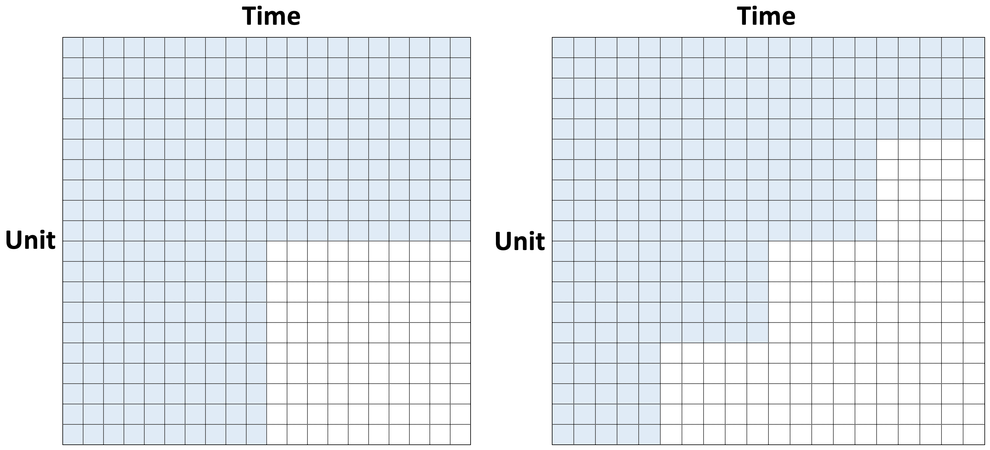
Situations when missing is not at random arise naturally in many causal panel models. Consider, for example, the evaluation of a program that takes effect after time T0T_{0} for the last N−N0N-N_{0} units. If MM is the potential outcome under the control, then we do not have observations of its entries for i>N0i>N_{0} and t>T0t>T_{0}, e.g., Ω=1{t≤T0ori≤N0}\Omega=1\{t\leq T_{0}{\rm\ or\ }i\leq N_{0}\}, yielding a block missing pattern as shown in the left panel of Figure 1. A more general setting that often arises in causal panel data is the staggered adoption where units may differ in the time they are first exposed to the treatment, yielding a missing pattern as shown in the right panel of Figure 1. See Athey et al., 2021; Agarwal et al., 2021 for other similar missing patterns that are common in the context of recommendation systems and A / B testing.
Refer to caption
Figure 1: Two typical observation patterns of the potential outcomes under the control in the causal panel model: Here, the blue area is the observed area, and the white area is the missing area. Missingness occurs because we cannot observe the potential outcomes under the control for the treated entries.

Note that if the entries are observed uniformly at random, then

‖Ω∘(Y−A)‖F2≈|Ω|N​T​𝔼​‖Y−A‖F2\|\Omega\circ(Y-A)\|_{\rm F}^{2}\approx{|\Omega|\over NT}{\mathbb{E}}\|Y-A\|_{\rm F}^{2}

for sufficiently large NN and TT. The right-hand side is minimized by MM, which justifies M~\widetilde{M} as a plausible estimate of MM. This intuition, however, no longer applies when Ω\Omega is not random and has more structured patterns. Our proposal to overcome this problem is dividing the missing entries into smaller groups and estimating each group via nuclear norm regularization. The main inspiration behind our method is the observation that M~\widetilde{M} is a good estimate of MM when there are only a few missing entries, even if they are missing not at random.

It is instructive to start with a single treated period, e.g., Ω=1{t≤T−1ori≤N0}\Omega=1\{t\leq T-1{\rm\ or\ }i\leq N_{0}\}. In this case, the number of missing entries is |Ωc|=N−N0|\Omega^{c}|=N-N_{0}. Denote by ψmax\psi_{\max} and ψmin\psi_{\min} the largest and smallest nonzero singular value of MM, respectively, and κ=ψmax/ψmin\kappa={\psi_{\max}}/{\psi_{\min}} its condition number. The following theorem provides bounds for the estimation error of M~\widetilde{M}.

Theorem 2.1.

Assume that

  • (i)

    σ​κ2​μ12​r12​max​{N​log⁡N,T​log⁡T}≪ψmin​min​{N,T}\sigma\kappa^{2}\mu^{\frac{1}{2}}r^{\frac{1}{2}}\max\{{N\sqrt{\log{N}}},{T\sqrt{\log{T}}}\}\ll\psi_{\min}\min\{\sqrt{N},\sqrt{T}\};

  • (ii)

    κ4​μ2​r2​max⁡{N​log3​N,T​log3​T}≪min⁡{N2,T2}\kappa^{4}\mu^{2}r^{2}\max\{{N\log^{3}{N}},{T\log^{3}{T}}\}\ll\min\{N^{2},T^{2}\};

  • (iii)

    |Ωc|​κ2​μ​r≪min⁡{N,T}|\Omega^{c}|\kappa^{2}\mu r\ll\min\{N,T\}.

Then, with probability at least 1−O⁡(min⁡{N−9,T−9})1-O(\min\{N^{-9},T^{-9}\}), we have

‖M~−M‖∞≤C​σ​μ​r32​κ2​max⁡{log⁡N,log⁡T}min⁡{N,T},\left\|\widetilde{M}-M\right\|_{\infty}\leq\frac{C\sigma\mu r^{\frac{3}{2}}\kappa^{2}\max\{\sqrt{\log N},\sqrt{\log T}\}}{\min\{\sqrt{N},\sqrt{T}\}},

for some absolute constant C>0C>0.

Some immediate remarks are in order. Consider the situation where κ,μ,r=O⁡(1)\kappa,\mu,r=O(1), and N≍TN\asymp T. Ignoring the logarithmic term, the signal-to-noise ratio requirement given by Assumption (i) reduces to ψmin≫σ​N1/2{\psi_{\min}}\gg\sigma N^{1/2} which is significantly weaker than those in the existing literature. More specifically, if there is a single missing entry, e.g., N0=N−1N_{0}=N-1, Agarwal et al., 2021 suggest to partition the submatrix (mi​t)1≤i<N,1≤t<T(m_{it})_{1\leq i<N,1\leq t<T} into KK smaller matrices. In particular, their Theorem 2 states that the best estimation error for their estimate is given by

|m^N​TADSS−mN​T|=Op​(1N1/4+1T1/4)|\widehat{m}^{\rm ADSS}_{NT}-m_{NT}|=O_{p}\left(\frac{1}{N^{1/4}}+\frac{1}{T^{1/4}}\right)

by setting K≍N1/2K\asymp N^{1/2}. In contrast, under the assumptions of Agarwal et al., 2021, σ,κ,μ,r\sigma,\kappa,\mu,r are bounded and hence the convergence rate of our estimator is

|m~N​T−mN​T|=Op​((1N1/2+1T1/2)​log⁡(N​T)).|\widetilde{m}_{NT}-m_{NT}|=O_{p}\left(\left(\frac{1}{N^{1/2}}+\frac{1}{T^{1/2}}\right)\sqrt{\log(NT)}\right).

Theorem 2.1 serves as our building block for dealing with more general and common missing patterns, which we shall now discuss in detail.

Single Treated Period.

Note that Assumption (iii) of Theorem 2.1 restricts the number of missing entries not to be large compared to NN and TT. In particular, if κ,μ,r=O⁡(1)\kappa,\mu,r=O(1) and N≍TN\asymp T, then it requires that |Ωc|=o⁡(N)|\Omega^{c}|=o\left(N\right). To deal with a larger number of missing entries, we shall leverage this result by splitting the missing entries into small groups and estimating them separately, as illustrated in Figure 2.

Refer to caption
Figure 2: How to construct the submatrix: We divide the missing entries into LL groups. For each 1≤l≤L1\leq l\leq L, we estimate the entries in 𝒢l\mathcal{G}_{l} using the nuclear norm penalized estimation on the submatrix YlY_{l} after making the submatrix YlY_{l} as described in the right panel.

Specifically, we split the missing entries into small groups, denoted by {𝒢l}1≤l≤L\{\mathcal{G}_{l}\}_{1\leq l\leq L}, and construct the submatrices {Yl}1≤l≤L\{Y_{l}\}_{1\leq l\leq L} as illustrated in Figure 2. For each 1≤l≤L1\leq l\leq L, we estimate MlM_{l}, the corresponding submatrix of MM, using the nuclear norm penalization:

M~l=arg​minA∈ℝNl×T⁡{‖Ωl∘(Yl−A)‖F2+λl​‖A‖∗},\displaystyle\widetilde{M}_{l}=\argmin_{A\in{\mathbb{R}}^{N_{l}\times T}}\left\{\|\Omega_{l}\circ(Y_{l}-A)\|_{\rm F}^{2}+\lambda_{l}\|A\|_{\ast}\right\}, (2.1)

where Nl=N0+|𝒢l|N_{l}=N_{0}+|\mathcal{G}_{l}| and Ωl\Omega_{l} is the corresponding submatrix of Ω\Omega. We shall then assemble these estimated submatrices into an estimate M~\widetilde{M} of MM. Note that each missing entry appears in one and only one of the submatrices and can therefore be estimated accordingly. The entries from OO in Figure 2, e.g., the N0×(T−1)N_{0}\times(T-1) principle submatrix of MM, on the other hand, are estimated for all groups. We can estimate these entries by averaging all of these estimates. Let the smallest nonzero singular value of MOM_{O} be ψmin,O\psi_{\min,O}, where MOM_{O} is the submatrix of MM corresponding to OO. Denote by ui⊤u_{i}^{\top} and vt⊤v_{t}^{\top} the ii-th row of UMU_{M} and tt-th row of VMV_{M}, respectively. We can then derive the following bounds from Theorem 2.1.

Corollary 2.2.

Assume that

  • (i)

    σ​κ94​μ12​r12​max​{N0​log⁡N0,T​log⁡T}≪ψmin,O​min​{N0,T}\sigma\kappa^{\frac{9}{4}}\mu^{\frac{1}{2}}r^{\frac{1}{2}}\max\{{N_{0}\sqrt{\log{N_{0}}}},{T\sqrt{\log{T}}}\}\ll\psi_{\min,O}\min\{\sqrt{N_{0}},\sqrt{T}\};

  • (ii)

    κ5​μ2​r2​max⁡{N0​log3​N0,T​log3​T}≪min⁡{N02,T2}\kappa^{5}\mu^{2}r^{2}\max\{{N_{0}\log^{3}{N_{0}}},{T\log^{3}{T}}\}\ll\min\{N_{0}^{2},T^{2}\};

  • (iii)

    |𝒢l|​κ52​μ​r≪min⁡{N0,T}|\mathcal{G}_{l}|\kappa^{\frac{5}{2}}\mu r\ll\min\{N_{0},T\}, l=1,…,Ll=1,\ldots,L;

  • (iv)

    There are constants C,c>0C,c>0 such that

    c≤λmin​(NN0​∑i≤N0ui​ui⊤)≤λmax​(NN0​∑i≤N0ui​ui⊤)≤C,c\leq\lambda_{\min}\left(\frac{N}{N_{0}}\sum_{i\leq N_{0}}u_{i}u_{i}^{\top}\right)\leq\lambda_{\max}\left(\frac{N}{N_{0}}\sum_{i\leq N_{0}}u_{i}u_{i}^{\top}\right)\leq C,

    where λmax​(A)\lambda_{\max}(A) and λmin​(A)\lambda_{\min}(A) are the largest and smallest singular value of AA, respectively.

Then, with probability at least 1−O⁡(min⁡{N0−9,T−9}​L)1-O(\min\{N_{0}^{-9},T^{-9}\}L), we have

‖M~−M‖∞≤C​σ​κ52​μ​r32​max⁡{log⁡N0,log⁡T}min⁡{N0,T},\left\|\widetilde{M}-M\right\|_{\infty}\leq C\frac{\sigma\kappa^{\frac{5}{2}}\mu r^{\frac{3}{2}}\max\{\sqrt{\log N_{0}},\sqrt{\log T}\}}{\min\{\sqrt{N_{0}},\sqrt{T}\}},

for some absolute constant C>0C>0.

The main difference from Theorem 2.1 lies in Assumptions (iii) and (iv) of Corollary 2.2. Assumption (iii) specifies how large a block can be. In principle, we can always take |𝒢l|=1|\mathcal{G}_{l}|=1, that is, recovering one entry at a time so that this condition is trivially satisfied with sufficiently large N0N_{0} and TT. However, there could be enormous computational advantages in creating groups as large as possible because the number of M~l\widetilde{M}_{l}s that need to be computed decreases with increasing group size.

Assumption (iv) can be viewed as an incoherence condition to ensure that the singular vectors of MM are not dominated by either the treated or untreated units. It is easy to see that when there are few missing entries, e.g., N0≈NN_{0}\approx N, the condition is satisfied by virtue of the incoherence of uiu_{i}s. In general, if {ui}i∈[N]\{u_{i}\}_{i\in[N]} is exchangeable or if the treated units are uniformly selected, then this condition is satisfied with high probability, at least for sufficiently large N0N_{0}, since NN0​∑i≤N0ui​ui⊤≈∑i≤Nui​ui⊤=Ir\frac{N}{N_{0}}\sum_{i\leq N_{0}}u_{i}u_{i}^{\top}\approx\sum_{i\leq N}u_{i}u_{i}^{\top}=I_{r} by means of matrix concentration inequalities (Tropp et al., 2015, see, e.g.,).

Single Treated Unit.

A similar estimating strategy can also be used to deal with a single treated unit. Without loss of generality, let Ω=1{t≤T0ori≤N−1}\Omega=1\{t\leq T_{0}{\rm\ or\ }i\leq N-1\}. Then the fully observed submatrix is O=(yi​t)1≤i≤N−1,1≤t≤T0O=(y_{it})_{1\leq i\leq N-1,1\leq t\leq T_{0}}. As in the case of a single treated period, we split the missing entries into smaller groups, denoted by 𝒢1,…,𝒢L\mathcal{G}_{1},\ldots,\mathcal{G}_{L}, by periods, and estimate them separately as before. Similar to Theorem 2.2, we have the following bounds for the resulting estimate.

Corollary 2.3.

Assume that

  • (i)

    σ​κ94​μ12​r12​max​{N​log⁡N,T0​log⁡T0}≪ψmin,O​min​{N,T0}\sigma\kappa^{\frac{9}{4}}\mu^{\frac{1}{2}}r^{\frac{1}{2}}\max\{{N\sqrt{\log{N}}},{T_{0}\sqrt{\log{T_{0}}}}\}\ll\psi_{\min,O}\min\{\sqrt{N},\sqrt{T_{0}}\};

  • (ii)

    κ5​μ2​r2​max⁡{N​log3​N,T0​log3​T0}≪min⁡{N2,T02}\kappa^{5}\mu^{2}r^{2}\max\{{N\log^{3}{N}},{T_{0}\log^{3}{T_{0}}}\}\ll\min\{N^{2},T_{0}^{2}\};

  • (iii)

    |𝒢l|​κ52​μ​r≪min⁡{N,T0}|\mathcal{G}_{l}|\kappa^{\frac{5}{2}}\mu r\ll\min\{N,T_{0}\}, l=1,…,Ll=1,\ldots,L;

  • (iv)

    There are constants C,c>0C,c>0 such that

    c≤λmin​(TT0​∑t≤T0vt​vt⊤)≤λmax​(TT0​∑t≤T0vt​vt⊤)≤C.c\leq\lambda_{\min}\left(\frac{T}{T_{0}}\sum_{t\leq T_{0}}v_{t}v_{t}^{\top}\right)\leq\lambda_{\max}\left(\frac{T}{T_{0}}\sum_{t\leq T_{0}}v_{t}v_{t}^{\top}\right)\leq C.

Then, with probability at least 1−O⁡(min⁡{N−9,T0−9}​L)1-O(\min\{N^{-9},T_{0}^{-9}\}L), we have

‖M~−M‖∞≤C​σ​κ52​μ​r32​max⁡{log⁡N,log⁡T0}min⁡{N,T0},\left\|\widetilde{M}-M\right\|_{\infty}\leq C\frac{\sigma\kappa^{\frac{5}{2}}\mu r^{\frac{3}{2}}\max\{\sqrt{\log N},\sqrt{\log T_{0}}\}}{\min\{\sqrt{N},\sqrt{T_{0}}\}},

for some absolute constant C>0C>0.

General Block Missing Pattern.

We can also apply the grouping and estimating procedure to general block missing structures such as that depicted in the left panel of Figure 1, e.g., Ω=1{t≤T0ori≤N0}\Omega=1\{t\leq T_{0}{\rm\ or\ }i\leq N_{0}\}, by estimating missing entries one period at a time (or one unit at a time). Denote by 𝒢1,𝒢2,…,𝒢L\mathcal{G}_{1},\mathcal{G}_{2},\ldots,\mathcal{G}_{L} the groups of missing units (or periods). The following result again follows from Theorem 2.1:

Corollary 2.4.

Assume that

  • (i)

    σ​κ94​μ12​r12​max​{N0​log⁡N0,T0​log⁡T0}≪ψmin,O​min​{N0,T0}\sigma\kappa^{\frac{9}{4}}\mu^{\frac{1}{2}}r^{\frac{1}{2}}\max\{{N_{0}\sqrt{\log{N_{0}}}},{T_{0}\sqrt{\log{T_{0}}}}\}\ll\psi_{\min,O}\min\{\sqrt{N_{0}},\sqrt{T_{0}}\};

  • (ii)

    κ5​μ2​r2​max⁡{N0​log3​N0,T0​log3​T0}≪min⁡{N02,T02}\kappa^{5}\mu^{2}r^{2}\max\{{N_{0}\log^{3}{N_{0}}},{T_{0}\log^{3}{T_{0}}}\}\ll\min\{N_{0}^{2},T_{0}^{2}\};

  • (iii)

    |𝒢l|​κ52​μ​r≪min⁡{N0,T0}|\mathcal{G}_{l}|\kappa^{\frac{5}{2}}\mu r\ll\min\{N_{0},T_{0}\}, l=1,…,Ll=1,\ldots,L;

  • (iv)

    There are constants C,c>0C,c>0 such that

    c≤λmin​(NN0​∑i≤N0ui​ui⊤)≤λmax​(NN0​∑i≤N0ui​ui⊤)≤C,\displaystyle c\leq\lambda_{\min}\left(\frac{N}{N_{0}}\sum_{i\leq N_{0}}u_{i}u_{i}^{\top}\right)\leq\lambda_{\max}\left(\frac{N}{N_{0}}\sum_{i\leq N_{0}}u_{i}u_{i}^{\top}\right)\leq C,
    c≤λmin​(TT0​∑t≤T0vt​vt⊤)≤λmax​(TT0​∑t≤T0vt​vt⊤)≤C.\displaystyle c\leq\lambda_{\min}\left(\frac{T}{T_{0}}\sum_{t\leq T_{0}}v_{t}v_{t}^{\top}\right)\leq\lambda_{\max}\left(\frac{T}{T_{0}}\sum_{t\leq T_{0}}v_{t}v_{t}^{\top}\right)\leq C.

Then, with probability at least 1−O⁡(min⁡{N0−9,T0−9}​L​(T−T0))1-O(\min\{N_{0}^{-9},T_{0}^{-9}\}L(T-T_{0})), we have

‖M~−M‖∞≤C​σ​κ52​μ​r32​max⁡{log⁡N0,log⁡T0}min⁡{N0,T0},\left\|\widetilde{M}-M\right\|_{\infty}\leq C\frac{\sigma\kappa^{\frac{5}{2}}\mu r^{\frac{3}{2}}\max\{\sqrt{\log N_{0}},\sqrt{\log T_{0}}\}}{\min\{\sqrt{N_{0}},\sqrt{T_{0}}\}},

for some absolute constant C>0C>0.

It is worth noting that both Corollary 2.2 and Corollary 2.3 can be viewed as special cases of Corollary 2.4. It is also of interest to compare the rates of convergence with those of Athey et al., 2021. Athey et al., 2021 considered a direct application of the nuclear norm penalized estimation to the full matrix. Their Theorem 2 states that

1N​T​‖M~−M‖F=Op​(TN+1T),\frac{1}{\sqrt{NT}}\left\|\widetilde{M}-M\right\|_{\rm F}=O_{p}\left(\sqrt{\frac{T}{N}}+\sqrt{\frac{1}{T}}\right),

ignoring the logarithmic factors and σ\sigma, rr, and ‖M‖∞\left\|M\right\|_{\infty}. In other words, the estimate could be inconsistent when N=O⁡(T)N=O(T). On the other hand, the convergence rate of our estimator is given by

‖M~−M‖∞=Op​(1N0+1T0),\left\|\widetilde{M}-M\right\|_{\infty}=O_{p}\left(\sqrt{\frac{1}{N_{0}}}+\sqrt{\frac{1}{T_{0}}}\right),

up to a logarithmic factor when we assume κ,μ=Op​(1)\kappa,\mu=O_{p}(1). Hence, our estimator is consistent as long as min⁡{N0,T0}\min\{N_{0},T_{0}\} diverges. Furthermore, the simulation results in Section 5 also show that applying the nuclear norm penalized estimation to the submatrix indeed performs much better than applying it to the full matrix as long as N0N_{0} and T0T_{0} are not too small.

Staggered Adoption.

More generally, we can take advantage of our estimation strategy for staggered adoption where there are DD number of adoption time points, says T1<⋯<TDT_{1}<\cdots<T_{D}, and DD number of corresponding groups of treated units, says G1,…,GDG_{1},\dots,G_{D}. That is, for each d∈[D]d\in[D], the units in GdG_{d} adopt the treatment in the time period TdT_{d}. We can utilize the strategy for block missing patterns to estimate the missing entries. More specifically, denote by Md,d′M_{d,d^{\prime}} the submatrix with missing entries corresponding to units in GdG_{d} and time periods in [Td′,Td′+1)[T_{d^{\prime}},T_{d^{\prime}+1}), with the convention that TD+1=T+1T_{D+1}=T+1, where d≤d′≤Dd\leq d^{\prime}\leq D. To estimate these missing entries, we can assemble a submatrix, denoted by Yd,d′Y_{d,d^{\prime}}, with units untreated prior to Td′+1T_{d^{\prime}+1} and time periods in [1,Td)∪[Td′,Td′+1)[1,T_{d})\cup[T_{d^{\prime}},T_{d^{\prime}+1}), as well as units in GdG_{d} and time periods in [1,Td)[1,T_{d}). As shown in Figure 3, Md,d′M_{d,d^{\prime}} is now the missing block of Yd,d′Y_{d,d^{\prime}}, and can be estimated as described in the previous case.

Denote by 𝒢1,𝒢2,…,𝒢L\mathcal{G}_{1},\mathcal{G}_{2},\ldots,\mathcal{G}_{L} the groups for missing units in Md,d′M_{d,d^{\prime}} such as ∪l∈[L]𝒢l=Gd\cup_{l\in[L]}\mathcal{G}_{l}=G_{d}, Nd′N_{d^{\prime}} the number of units that are untreated prior to Td′+1T_{d^{\prime}+1}, and ψmin,Od,d′\psi_{\min,O_{d,d^{\prime}}} the smallest singular value of the submatrix MOd,d′=(mi​t)1≤i≤Nd′,1≤t≤TdM_{O_{d,d^{\prime}}}=(m_{it})_{1\leq i\leq N_{d^{\prime}},1\leq t\leq T_{d}}. The performance of the resulting estimate is given by Corollary 2.5.

Refer to caption
Figure 3: How to construct the general block missing pattern: Consider the case of d=1d=1 and d′=2d^{\prime}=2. When we estimate the missing entries in M1,2M_{1,2}, we make the block missing matrix Y1,2Y_{1,2} by assembling four red matrices. Then, we can estimate the missing entries in M1,2M_{1,2} using the estimation method for the general block missing pattern.
Corollary 2.5.

Assume that

  • (i)

    σ​κ94​μ12​r12​max​{Nd′​log⁡Nd′,Td​log⁡Td}≪ψmin,Od,d′​min​{Nd′,Td}\sigma\kappa^{\frac{9}{4}}\mu^{\frac{1}{2}}r^{\frac{1}{2}}\max\{{N_{d^{\prime}}\sqrt{\log{N_{d^{\prime}}}}},{T_{d}\sqrt{\log{T_{d}}}}\}\ll\psi_{\min,O_{d,d^{\prime}}}\min\{\sqrt{N_{d^{\prime}}},\sqrt{T_{d}}\};

  • (ii)

    κ5​μ2​r2​max⁡{Nd′​log3​Nd′,Td​log3​Td}≪min⁡{Nd′2,Td2}\kappa^{5}\mu^{2}r^{2}\max\{{N_{d^{\prime}}\log^{3}{N_{d^{\prime}}}},{T_{d}\log^{3}{T_{d}}}\}\ll\min\{N_{d^{\prime}}^{2},T_{d}^{2}\};

  • (iii)

    |𝒢l|​κ52​μ​r≪min⁡{Nd′,Td}|\mathcal{G}_{l}|\kappa^{\frac{5}{2}}\mu r\ll\min\{N_{d^{\prime}},T_{d}\}, l=1,…,Ll=1,\ldots,L;

  • (iv)

    There are constants C,c>0C,c>0 such that

    c≤λmin​(NNd′​∑i≤Nd′ui​ui⊤)≤λmax​(NNd′​∑i≤Nd′ui​ui⊤)≤C,\displaystyle c\leq\lambda_{\min}\left(\frac{N}{N_{d^{\prime}}}\sum_{i\leq N_{d^{\prime}}}u_{i}u_{i}^{\top}\right)\leq\lambda_{\max}\left(\frac{N}{N_{d^{\prime}}}\sum_{i\leq N_{d^{\prime}}}u_{i}u_{i}^{\top}\right)\leq C,
    c≤λmin​(TTd​∑t≤Tdvt​vt⊤)≤λmax​(TTd​∑t≤Tdvt​vt⊤)≤C.\displaystyle c\leq\lambda_{\min}\left(\frac{T}{T_{d}}\sum_{t\leq T_{d}}v_{t}v_{t}^{\top}\right)\leq\lambda_{\max}\left(\frac{T}{T_{d}}\sum_{t\leq T_{d}}v_{t}v_{t}^{\top}\right)\leq C.

Then, with probability at least 1−O⁡(min⁡{Nd′−9,Td−9}​L​(Td′+1−Td′))1-O(\min\{N_{d^{\prime}}^{-9},T_{d}^{-9}\}L(T_{d^{\prime}+1}-T_{d^{\prime}})), we have

‖M~d,d′−Md,d′‖∞≤C​σ​κ52​μ​r32​max⁡{log⁡Nd′,log⁡Td}min⁡{Nd′,Td},\left\|\widetilde{M}_{d,d^{\prime}}-M_{d,d^{\prime}}\right\|_{\infty}\leq C\frac{\sigma\kappa^{\frac{5}{2}}\mu r^{\frac{3}{2}}\max\{\sqrt{\log N_{d^{\prime}}},\sqrt{\log T_{d}}\}}{\min\{\sqrt{N_{d^{\prime}}},\sqrt{T_{d}}\}},

for some absolute constant C>0C>0.

It is worth comparing the rates of convergence with those of Bai and Ng, 2021 which apply their TW algorithm to the full matrix. For all missing entries, the convergence rates of the estimators in Bai and Ng, 2021 are Op​(1ND+1T1)O_{p}\left(\frac{1}{\sqrt{N_{D}}}+\frac{1}{\sqrt{T_{1}}}\right). On the other hand, if we assume κ,μ=Op​(1)\kappa,\mu=O_{p}(1), the convergence rate of our estimator is Op​(1Nd′+1Td)O_{p}\left(\frac{1}{\sqrt{N_{d^{\prime}}}}+\frac{1}{\sqrt{T_{d}}}\right) up to a logarithmic factor. Since Nd′>NDN_{d^{\prime}}>N_{D} and Td>T1T_{d}>T_{1} for all d′<Dd^{\prime}<D and d>1d>1, our convergence rate is faster than that of Bai and Ng, 2021 except for the estimation of missing entries in part M1,DM_{1,D} for which both estimates have similar rates of convergence. This shows the advantage of exploiting submatrices for the imputation of missing entries.

3 Debiasing and Statistical Inferences

We now turn our attention to inferences. While the nuclear norm regularized estimator M~\widetilde{M} enjoys good rates of convergence, it is not directly suitable for statistical inferences due to the bias induced by the penalty. To overcome this challenge, we propose an additional projection step after applying the nuclear norm penalization in recovering missing entries from group 𝒢l\mathcal{G}_{l}:

M^l=𝒫r​(Ωlc∘M~l+Ωl∘Yl),\widehat{M}_{l}=\mathcal{P}_{r}\left(\Omega^{c}_{l}\circ\widetilde{M}_{l}+\Omega_{l}\circ Y_{l}\right), (3.1)

where 𝒫r(B)=arg​minA:rank​(A)≤r‖A−B‖F\mathcal{P}_{r}(B)=\argmin_{A:\textrm{rank}(A)\leq r}\left\|A-B\right\|_{F} is the best rank-rr approximation of BB. We now discuss how this enables us to develop an inferential theory for estimating the missing entries. To fix ideas, we shall focus on inferences about the average of a group of entries at a given time period, e.g., ∑i∈𝒢mi​t0/|𝒢|\sum_{i\in\mathcal{G}}m_{it_{0}}/|\mathcal{G}|, where 𝒢⊆[N]\mathcal{G}\subseteq[N].

Block Missing Patterns.

We shall begin with general block missing patterns, e.g., ωi​t=1\omega_{it}=1 if t≤T0t\leq T_{0} or i≤N0i\leq N_{0}. Note that both the single treated period and single treated unit examples from the previous section can be viewed as special cases with T0=T−1T_{0}=T-1 and N0=N−1N_{0}=N-1, respectively.

Suppose that we are interested in the inference of the average of a group of entries at the time t0t_{0}, ∑i∈𝒢mi​t0/|𝒢|\sum_{i\in\mathcal{G}}m_{it_{0}}/|\mathcal{G}|, where 𝒢⊆{1,⋯,N}\mathcal{G}\subseteq\{1,\cdots,N\} and t0>T0t_{0}>T_{0}. Similar to before, we split the interesting group, 𝒢\mathcal{G}, into smaller subgroups, denoted by {𝒢l}0≤l≤L\{\mathcal{G}_{l}\}_{0\leq l\leq L} with the convention that 𝒢0=𝒢∩{1,⋯,N0}\mathcal{G}_{0}=\mathcal{G}\cap\{1,\cdots,N_{0}\}, and construct the corresponding submatrices {Yl}1≤l≤L\{Y_{l}\}_{1\leq l\leq L} as illustrated in Figure 4, and construct Y0=[(yi​t)i≤N0,t≤T0(yi​t)i≤N0,t=t0]Y_{0}=[(y_{it})_{i\leq N_{0},t\leq T_{0}}\ \ (y_{it})_{i\leq N_{0},t=t_{0}}] if 𝒢0≠∅\mathcal{G}_{0}\neq\emptyset.

Refer to caption
Figure 4: How to construct the submatrix: The blue area is the observed area and the white area is the missing area. We estimate the entries in 𝒢l\mathcal{G}_{l} using the submatrix YlY_{l} as described in the figure.

Recall that ψmin,O\psi_{\min,O} is the smallest nonzero singular value of the N0×T0N_{0}\times T_{0} matrix MO=(mi​t)1≤i≤N0,1≤t≤T0M_{O}=(m_{it})_{1\leq i\leq N_{0},1\leq t\leq T_{0}}. The following theorem establishes the asymptotic normality of the group average estimator, ∑i∈𝒢m^i​t0/|𝒢|\sum_{i\in\mathcal{G}}\widehat{m}_{it_{0}}/|\mathcal{G}|.

Theorem 3.1.

Assume that

  • (i)

    σ​κ234​μ32​r32​min​{N0,|𝒢|​T0}​max​{N0​log⁡N0,T0​log⁡T0}=op​(ψmin,O​min​{N0,T0})\sigma\kappa^{\frac{23}{4}}\mu^{\frac{3}{2}}r^{\frac{3}{2}}\min\{\sqrt{N_{0}},\sqrt{|\mathcal{G}|T_{0}}\}\max\{{N_{0}\sqrt{\log{N_{0}}}},{T_{0}\sqrt{\log{T_{0}}}}\}=o_{p}\left(\psi_{\min,O}\min\{N_{0},T_{0}\}\right);

  • (ii)

    κ112​μ3​r3​min⁡{N0,|𝒢|​T0}​max​{N0​log3​N0,T0​log3​T0}=op​(min⁡{N032,T032})\kappa^{\frac{11}{2}}\mu^{3}r^{3}\min\{\sqrt{N_{0}},\sqrt{|\mathcal{G}|T_{0}}\}\max\{{\sqrt{N_{0}\log^{3}{N_{0}}}},{\sqrt{T_{0}\log^{3}{T_{0}}}}\}=o_{p}\left(\min\{N_{0}^{\frac{3}{2}},T_{0}^{\frac{3}{2}}\}\right);

  • (iii)

    |𝒢l|​κ174​μ52​r52​max​{N0​log⁡N0,T0​log⁡T0}=op​(N0​min​{N0,T0})|\mathcal{G}_{l}|\kappa^{\frac{17}{4}}\mu^{\frac{5}{2}}r^{\frac{5}{2}}\max\{\sqrt{N_{0}\log{N_{0}}},\sqrt{T_{0}\log{T_{0}}}\}=o_{p}\left(\sqrt{N_{0}}\min\{N_{0},T_{0}\}\right), l=1,…,Ll=1,\ldots,L;

  • (iv)

    There are constants C,c>0C,c>0 such that

    c≤λmin​(NN0​∑i≤N0ui​ui⊤)≤λmax​(NN0​∑i≤N0ui​ui⊤)≤C,\displaystyle c\leq\lambda_{\min}\left(\frac{N}{N_{0}}\sum_{i\leq N_{0}}u_{i}u_{i}^{\top}\right)\leq\lambda_{\max}\left(\frac{N}{N_{0}}\sum_{i\leq N_{0}}u_{i}u_{i}^{\top}\right)\leq C,
    c≤λmin​(TT0​∑t≤T0vt​vt⊤)≤λmax​(TT0​∑t≤T0vt​vt⊤)≤C;\displaystyle c\leq\lambda_{\min}\left(\frac{T}{T_{0}}\sum_{t\leq T_{0}}v_{t}v_{t}^{\top}\right)\leq\lambda_{\max}\left(\frac{T}{T_{0}}\sum_{t\leq T_{0}}v_{t}v_{t}^{\top}\right)\leq C;
  • (v)

    N​‖u¯𝒢‖≥c\sqrt{N}\left\|\bar{u}_{\mathcal{G}}\right\|\geq c and T​‖vt0‖≥c\sqrt{T}\left\|v_{t_{0}}\right\|\geq c for some constant c>0c>0 where u¯𝒢=|𝒢|−1​∑i∈𝒢ui\bar{u}_{\mathcal{G}}=|\mathcal{G}|^{-1}\sum_{i\in\mathcal{G}}u_{i}.

Then, we have

𝒱𝒢−12​(1|𝒢|​∑i∈𝒢m^i​t0−1|𝒢|​∑i∈𝒢mi​t0)​⟶𝐷​𝒩​(0,1),\displaystyle\mathcal{V}_{\mathcal{G}}^{-\frac{1}{2}}\left(\frac{1}{|\mathcal{G}|}\sum_{i\in\mathcal{G}}\widehat{m}_{it_{0}}-\frac{1}{|\mathcal{G}|}\sum_{i\in\mathcal{G}}m_{it_{0}}\right)\overset{D}{\longrightarrow}\mathcal{N}(0,1),

where

𝒱𝒢=σ2​(u¯𝒢⊤​(∑j≤N0uj​uj⊤)−1​u¯𝒢+1|𝒢|​vt0⊤​(∑s≤T0vs​vs⊤)−1​vt0).\mathcal{V}_{\mathcal{G}}=\sigma^{2}\left(\bar{u}_{\mathcal{G}}^{\top}\left(\sum_{j\leq N_{0}}u_{j}u_{j}^{\top}\right)^{-1}\bar{u}_{\mathcal{G}}+\frac{1}{|\mathcal{G}|}v_{t_{0}}^{\top}\left(\sum_{s\leq T_{0}}v_{s}v_{s}^{\top}\right)^{-1}v_{t_{0}}\right).

Staggered Adaption.

More generally, consider the case of staggered adoption when there are DD number of adoption time points, T1<T2<⋯<TDT_{1}<T_{2}<\cdots<T_{D}, and DD number of corresponding groups of treated units, G1,…,GDG_{1},\ldots,G_{D}. As in the previous situation, suppose that we are interested in inference for the group average at time t0t_{0}. Denote by N0N_{0} the number of units that are untreated until t0t_{0}, and by T0T_{0} the number of time periods where {1,…,N0}\{1,\dots,N_{0}\} is untreated, respectively.

We proceed by first splitting 𝒢\mathcal{G} into smaller groups, denoted by {𝒢l}0≤l≤L\{\mathcal{G}_{l}\}_{0\leq l\leq L} with the convention that 𝒢0=𝒢∩{1,⋯,N0}\mathcal{G}_{0}=\mathcal{G}\cap\{1,\cdots,N_{0}\}. In doing so, we want to make sure that all units in each subgroup {𝒢l}1≤l≤L\{\mathcal{G}_{l}\}_{1\leq l\leq L} have the same adoption time point, e.g., 𝒢l⊆Gdl\mathcal{G}_{l}\subseteq G_{d_{l}}, as illustrated in Figure 5. Denote by D𝒢={dl:1≤l≤L}D_{\mathcal{G}}=\{d_{l}:1\leq l\leq L\} and by ψmin,Od\psi_{\min,O_{d}} the smallest singular value of the submatrix MOd=(mi​t)1≤i≤N0,1≤t≤TdM_{O_{d}}=(m_{it})_{1\leq i\leq N_{0},1\leq t\leq T_{d}}.

Refer to caption
Figure 5: Submatrix construction: For each 1≤l≤31\leq l\leq 3, we make the submatrix YlY_{l} by putting OlO_{l}, plp_{l}, qq, and 𝒢l\mathcal{G}_{l} together. In addition, we estimate the entries in 𝒢0\mathcal{G}_{0} using the fully observed part Y0=(yi​t)1≤i≤N0,1≤t≤T0Y_{0}=(y_{it})_{1\leq i\leq N_{0},1\leq t\leq T_{0}}.
Theorem 3.2.

Assume that for any d∈D𝒢∪{0}d\in D_{\mathcal{G}}\cup\{0\} and l=1,…,Ll=1,\ldots,L,

  • (i)

    σ​κ234​μ32​r32​N0​max​{N0​log⁡N0,Td​log⁡Td}=op​(ψmin,Od​min​{N0,Td})\sigma\kappa^{\frac{23}{4}}\mu^{\frac{3}{2}}r^{\frac{3}{2}}\sqrt{N_{0}}\max\{{N_{0}\sqrt{\log{N_{0}}}},{T_{d}\sqrt{\log{T_{d}}}}\}=o_{p}\left(\psi_{\min,O_{d}}\min\{N_{0},T_{d}\}\right);

  • (ii)

    κ112​μ3​r3​N0​max⁡{N0​log3​N0,Td​log3​Td}=op​(min⁡{N032,Td32})\kappa^{\frac{11}{2}}\mu^{3}r^{3}\sqrt{N_{0}}\max\{{\sqrt{N_{0}\log^{3}{N_{0}}}},{\sqrt{T_{d}\log^{3}{T_{d}}}}\}=o_{p}\left(\min\{N_{0}^{\frac{3}{2}},T_{d}^{\frac{3}{2}}\}\right);

  • (iii)

    |𝒢l|​κ174​μ52​r52​max​{N0​log⁡N0,Tdl​log⁡Tdl}=op​(N0​min​{N0,Tdl})|\mathcal{G}_{l}|\kappa^{\frac{17}{4}}\mu^{\frac{5}{2}}r^{\frac{5}{2}}\max\{\sqrt{N_{0}\log{N_{0}}},\sqrt{T_{d_{l}}\log{T_{d_{l}}}}\}=o_{p}\left(\sqrt{N_{0}}\min\{N_{0},T_{d_{l}}\}\right);

  • (iv)

    there are constants C,c>0C,c>0 such that

    c≤λmin​(NN0​∑i≤N0ui​ui⊤)≤λmax​(NN0​∑i≤N0ui​ui⊤)≤C,\displaystyle c\leq\lambda_{\min}\left(\frac{N}{N_{0}}\sum_{i\leq N_{0}}u_{i}u_{i}^{\top}\right)\leq\lambda_{\max}\left(\frac{N}{N_{0}}\sum_{i\leq N_{0}}u_{i}u_{i}^{\top}\right)\leq C,
    c≤λmin​(TTd​∑t≤Tdvt​vt⊤)≤λmax​(TTd​∑t≤Tdvt​vt⊤)≤C;\displaystyle c\leq\lambda_{\min}\left(\frac{T}{T_{d}}\sum_{t\leq T_{d}}v_{t}v_{t}^{\top}\right)\leq\lambda_{\max}\left(\frac{T}{T_{d}}\sum_{t\leq T_{d}}v_{t}v_{t}^{\top}\right)\leq C;
  • (v)

    N​‖u¯𝒢‖≥c\sqrt{N}\left\|\bar{u}_{\mathcal{G}}\right\|\geq c and T​‖vt0‖≥c\sqrt{T}\left\|v_{t_{0}}\right\|\geq c for some constant c>0c>0.

Then, we have

𝒱𝒢−12​(1|𝒢|​∑i∈𝒢m^i​t0−1|𝒢|​∑i∈𝒢mi​t0)​⟶𝐷​𝒩​(0,1),\displaystyle\mathcal{V}_{\mathcal{G}}^{-\frac{1}{2}}\left(\frac{1}{|\mathcal{G}|}\sum_{i\in\mathcal{G}}\widehat{m}_{it_{0}}-\frac{1}{|\mathcal{G}|}\sum_{i\in\mathcal{G}}m_{it_{0}}\right)\overset{D}{\longrightarrow}\mathcal{N}(0,1),

where

𝒱𝒢=σ2​(u¯𝒢⊤​(∑j≤N0uj​uj⊤)−1​u¯𝒢+1|𝒢|​vt0⊤​[∑d∈D𝒢∪{0}|Gd∩𝒢||𝒢|​(∑s≤Tdvs​vs⊤)−1]​vt0),\mathcal{V}_{\mathcal{G}}=\sigma^{2}\left(\bar{u}_{\mathcal{G}}^{\top}\left(\sum_{j\leq N_{0}}u_{j}u_{j}^{\top}\right)^{-1}\bar{u}_{\mathcal{G}}+\frac{1}{|\mathcal{G}|}v_{t_{0}}^{\top}\left[\sum_{d\in D_{\mathcal{G}}\cup\{0\}}\frac{|G_{d}\cap\mathcal{G}|}{|\mathcal{G}|}\left(\sum_{s\leq T_{d}}v_{s}v_{s}^{\top}\right)^{-1}\right]v_{t_{0}}\right),

with the convention that G0={1,…,N0}G_{0}=\{1,\dots,N_{0}\}.

Variance Estimation.

In practice, to use the results above for inferences, we also need to estimate the variance. To this end, let U~l​D~l​V~l⊤\widetilde{U}_{l}\widetilde{D}_{l}\widetilde{V}_{l}^{\top} be the SVD of 𝒫r​(M~l)\mathcal{P}_{r}(\widetilde{M}_{l}). Denote by X~l=U~l​D~l1/2\widetilde{X}_{l}=\widetilde{U}_{l}\widetilde{D}_{l}^{1/2} and Z~l=V~l​D~l1/2\widetilde{Z}_{l}=\widetilde{V}_{l}\widetilde{D}_{l}^{1/2}. They can be viewed as estimates of rescaled left and right singular vectors. However, as such, they are significantly biased and the bias can be reduced by considering instead

X^l=X~l​(Ir+λl​(X~l⊤​X~l))1/2,Z^l=Z~l​(Ir+λl​(Z~l⊤​Z~l))1/2.\widehat{X}_{l}=\widetilde{X}_{l}\left(I_{r}+\lambda_{l}(\widetilde{X}_{l}^{\top}\widetilde{X}_{l})\right)^{1/2},\ \ \widehat{Z}_{l}=\widetilde{Z}_{l}\left(I_{r}+\lambda_{l}(\widetilde{Z}_{l}^{\top}\widetilde{Z}_{l})\right)^{1/2}.

We can then use X^l\widehat{X}_{l} and Z^l\widehat{Z}_{l} in place of the left and right singular vector in defining 𝒱𝒢\mathcal{V}_{\mathcal{G}}, leading to the following variance estimate

𝒱^𝒢=σ^2​∑i≤N0(∑0≤l≤L|𝒢l||𝒢|​X¯^𝒢l⊤​(∑j≤N0X^l,j​X^l,j⊤)−1​X^l,i)2\displaystyle\widehat{\mathcal{V}}_{\mathcal{G}}=\widehat{\sigma}^{2}\sum_{i\leq N_{0}}\left(\sum_{0\leq l\leq L}\frac{|\mathcal{G}_{l}|}{|\mathcal{G}|}\widehat{\bar{X}}_{\mathcal{G}_{l}}^{\top}\left(\sum_{j\leq N_{0}}\widehat{X}_{l,j}\widehat{X}_{l,j}^{\top}\right)^{-1}\widehat{X}_{l,i}\right)^{2}
+σ^2|𝒢|∑0≤l≤L|𝒢l||𝒢|Z^t0⊤(∑s≤TdlZ^l,sZ^l,s⊤)−1Z^l,t0,\displaystyle+\frac{\widehat{\sigma}^{2}}{|\mathcal{G}|}\sum_{0\leq l\leq L}\frac{|\mathcal{G}_{l}|}{|\mathcal{G}|}\widehat{Z}_{t_{0}}^{\top}\left(\sum_{s\leq T_{d_{l}}}\widehat{Z}_{l,s}\widehat{Z}_{l,s}^{\top}\right)^{-1}\widehat{Z}_{l,t_{0}},

where X¯^𝒢l=1|𝒢l|​∑j∈𝒢lX^l,j\widehat{\bar{X}}_{\mathcal{G}_{l}}=\frac{1}{|\mathcal{G}_{l}|}\sum_{j\in\mathcal{G}_{l}}\widehat{X}_{l,j}, σ^2=1N0​T0​∑i≤N0,t≤T0ϵ^i​t2\widehat{\sigma}^{2}=\frac{1}{N_{0}T_{0}}\sum_{i\leq N_{0},t\leq T_{0}}\widehat{\epsilon}_{it}^{2}, and ϵ^i​t=yi​t−m^i​t\widehat{\epsilon}_{it}=y_{it}-\widehat{m}_{it}. The following corollary shows that asymptotic normality established in Theorem 3.2 continues to hold if we use this variance estimate.

Corollary 3.3.

Suppose that the assumptions in Theorem 3.2 hold. In addition, suppose that for any d∈D𝒢∪{0}d\in D_{\mathcal{G}}\cup\{0\},

σ​κ5​μ3​r3​N0​max​{N0​log⁡N0,Td​log⁡Td}=op​(ψmin,Od​min​{N0,Td}).\sigma\kappa^{5}\mu^{3}r^{3}N_{0}\max\{\sqrt{N_{0}\log N_{0}},\sqrt{T_{d}\log T_{d}}\}=o_{p}\left(\psi_{\min,O_{d}}\min\{N_{0},T_{d}\}\right).

Then

𝒱^𝒢−12​(1|𝒢|​∑i∈𝒢m^i​t0−1|𝒢|​∑i∈𝒢mi​t0)​⟶𝐷​𝒩​(0,1).\widehat{\mathcal{V}}_{\mathcal{G}}^{-\frac{1}{2}}\left(\frac{1}{|\mathcal{G}|}\sum_{i\in\mathcal{G}}\widehat{m}_{it_{0}}-\frac{1}{|\mathcal{G}|}\sum_{i\in\mathcal{G}}m_{it_{0}}\right)\overset{D}{\longrightarrow}\mathcal{N}(0,1).

Since Theorem 3.1 is a special case of Theorem 3.2, the variance estimator can also be used for Theorem 3.1. Specifically, it is enough to change from TdlT_{d_{l}} in 𝒱^𝒢\widehat{\mathcal{V}}_{\mathcal{G}} to T0T_{0} for Theorem 3.1.

4 Application to Tick Size Pilot Program

Our work was motivated by the analysis of the Tick Size Pilot Program, which we shall now discuss in detail to demonstrate how the proposed methodology can be applied in causal panel data models.

4.1 Data and Methods

Background.

In October 2016, the SEC launched the Tick Size Pilot Program to evaluate the impact of an increase in tick sizes on the market quality of stocks. As noted before, the pilot consisted of a control group and three treatment groups:

  1. Control.

    stocks in the control group was quoted and traded in $0.01 increments;

  2. Q rule.

    stocks in the Q rule group was quoted in $0.05 increments but still traded in $0.01 increments;

  3. Q+T rule.

    stocks in this rule group was quoted and traded in $0.05 increments;

  4. Q+T+TA rule.

    stocks in this group are also subject to the additional trade-at rule, a regulation which makes exchanges display the NBBO (National Best Bid and Offer) when they execute a trade at the NBBO.

This pilot program has attracted considerable attention, and there are a growing number of studies on the impact of these changes on market quality, often represented by a liquidity measure such as the effective spread since its conclusion in 2018. See, e.g., Albuquerque et al., 2020; Chung et al., 2020; Griffith and Roseman, 2019; Rindi and Werner, 2019; Werner et al., 2022.

Data.

Data for control variables were obtained from the Center for Research in Security Prices (CRSP) and the daily share-weighted dollar effective spread data from the Millisecond Intraday Indicators by Wharton Research Data Services (WRDS). A key control variable introduced by Chung et al., 2020 is TBC which measures the extent to which the new tick size ($0.05) is a binding constraint on the quoted spreads in the pilot periods and is estimated by the percentage of quoted spreads during the day that are equal to or less than 5 cents, which is the new minimum quoted tick size under the Q rule. Specifically, we calculate the percentage of NBBO updates with quoted spread less than or equal to 5 cents for each day. Using the TBC variable, we can check the effect of an increase in the minimum quoted spread (from 1 cent to 5 cents) on the effective spread.

A data-cleaning process similar to Chung et al., 2020 yields a total of N=1,461N=1,461 stocks with N0=735N_{0}=735 in the control group, N1=254N_{1}=254 in the Q group, N2=244N_{2}=244 in the Q+T group, and N3=228N_{3}=228 in the Q+T+TA group. Following Chung et al., 2020, data from Oct 1, 2015 to Sep 30, 2016 were used as the pre-pilot periods and Nov 1, 2016 to Oct 31, 2017 as the pilot periods, i.e., T0=253T_{0}=253 and T1=252T_{1}=252 for daily data. See Chung et al., 2020 for further discussion of data collection. As is common in previous studies, we consider the daily effective spread in cents as a measure of liquidity. Denote by yi​t(d)y_{it}^{(d)} the potential outcome for stock ii at time tt under treatment dd with the convention that d=0,1,2,3d=0,1,2,3 corresponds to the control, the Q rule, the Q + T rule, and the Q + T + TA rule, respectively. The four matrices Y(d)=(yi​t(d))1≤i≤N,1≤t≤TY^{(d)}=(y_{it}^{(d)})_{1\leq i\leq N,1\leq t\leq T} have block missing patterns, as shown in Figure 6.

Refer to caption
Figure 6: Missing pattern in the pilot program: The blue area is the observed area and the white area is the missing area. In the case of the controlled situation (d=0d=0), we can observe the outcomes of all units in the pre-pilot periods and those of the control group in the pilot periods. In the case of the treated situation by the treatment dd, we can only observe the outcomes of the treatment group ℐd\mathcal{I}_{d} in the pilot periods.

Model.

Previous studies of the effects of the quote (Q) rule, the trade (T) rule, and the trade-at (TA) rule on the liquidity measure are usually based on traditional regression or difference-in-difference methods by assuming that the treatment effect is constant across all units and time periods. For instance, Chung et al., 2020 postulated yi​t=yi​t(d)y_{it}=y_{it}^{(d)} if unit ii receives treatment dd at time tt where the potential outcomes

yi​t(d)=mi​t(d)+xi​t⊤​β+ϵi​ty_{it}^{(d)}=m_{it}^{(d)}+x_{it}^{\top}\beta+\epsilon_{it}

and

mi​t(d)=μ(d)+αi+δt.m_{it}^{(d)}=\mu^{(d)}+\alpha_{i}+\delta_{t}. (4.1)

Here, μ(0)=0\mu^{(0)}=0, μ(1),μ(2),μ(3)\mu^{(1)},\mu^{(2)},\mu^{(3)}, αi\alpha_{i}s and δt\delta_{t}s are unknown parameters, and xi​tx_{it} is a set of control variables that includes typical stock characteristics like stock prices and trading volumes, and TBC, a variable measuring the extent to which the new tick size ($0.05) is a binding constraint on the quoted spreads in the pilot period. See Section E in the Appendix for further details. It is worth noting that, in addition to the treatment effects (μ(1)\mu^{(1)}, μ(2)\mu^{(2)} and μ(3)\mu^{(3)}), their differences θ(d):=μ(d)−μ(d−1)\theta^{(d)}:=\mu^{(d)}-\mu^{(d-1)} are also of interest, as they represent the treatment effects of quote rule, trade rule, and trade-at rule, respectively.

However, (4.1) fails to account for the significant heterogeneity in the treatment effects across units and time periods. To this end, we shall consider a more flexible model:

mi​t(d)=ζi⊤ηt(d),d=0,1,2,3,m_{it}^{(d)}=\zeta_{i}^{\top}\eta_{t}^{(d)},\qquad{d=0,1,2,3}, (4.2)

where ζi\zeta_{i} is a rr-dimensional vector of (latent) unit specific characteristics and ηt(d)\eta_{t}^{(d)} is the corresponding coefficients of ζi\zeta_{i} at time tt in the potential situation dd. As we shall see later in this section, (4.2) allows us to get more insights into the treatment effects of the pilot program.

One of the key assumptions of Model (4.2) is that the subspace spanned by the left singular vector of M(d)=(mi​t(d))1≤i≤N,1≤t≤TM^{(d)}=(m_{it}^{(d)})_{1\leq i\leq N,1\leq t\leq T} for all d=1,2,3d=1,2,3 is included in the subspace spanned by the left singular vector of M(0)M^{(0)}. Agarwal et al., 2020 propose a subspace inclusion test to check the validity of this assumption. We carried out this test on the pilot data, which confirms this is a reasonable assumption.

We note that similar low-rank models have also been considered by Agarwal et al., 2020 and Chernozhukov et al., 2021 earlier. However, it is unclear how their methodology can be adapted for the analysis of the Tick Size Program. For example, Chernozhukov et al., 2021 impose conditions on the missing pattern that are clearly violated by the pilot data; Agarwal et al., 2020 only study the average treatment effect and so cannot be used to assess the heterogeneity or dynamics of the treatment effects across units and time periods, respectively.

Estimation.

We now discuss how we can apply the methodology in the previous sections to analyze the tick size program, and in particular to estimate and make inferences about (4.2). More specifically, we are interested in estimating the group-averaged treatment effects: for an interesting group of treated units 𝒢\mathcal{G},

μt(d):=1|𝒢|​∑i∈𝒢[mi​t(d)−mi​t(0)],\mu^{(d)}_{t}:={1\over|\mathcal{G}|}\sum_{i\in\mathcal{G}}[m^{(d)}_{it}-m^{(0)}_{it}],

and their differences:

θt(d):=μt(d)−μt(d−1),\theta^{(d)}_{t}:=\mu^{(d)}_{t}-\mu^{(d-1)}_{t},

for t>T0t>T_{0}. Especially, when 𝒢\mathcal{G} is a certain unit, it reduces to the individual treatment effect and if 𝒢\mathcal{G} is the group of all treated units, it becomes the cross-sectional averaged treatment effect. To this end, we shall derive estimates for mi​t(d)m^{(d)}_{it} under Model (4.2).

First, note that, for this particular application, one of the covariates (TBC) is only present for the pilot periods. Therefore, we cannot hope to estimate the regression coefficient β\beta using the pre-pilot data alone, as suggested by Bai and Ng, 2021. Nonetheless, under (4.2), yi​ty_{it}s follow an interactive fixed effect model:

yi​t=xi​t⊤​β+Li​t+ϵi​ty_{it}=x_{it}^{\top}\beta+L_{it}+\epsilon_{it}

for some low rank components Li​tL_{it} and therefore the regression coefficient β\beta can be estimated at the rate of Op​(1/N​T)O_{p}(1/\sqrt{NT}). See Bai, 2009 for details. This is much faster than that of the estimates of mi​t(d)m^{(d)}_{it}. For brevity, we shall, therefore, treat the regression coefficient β\beta as known in what follows, without loss of generality.

For d=0d=0, we can apply the method proposed in the previous sections to the potential outcome panel Y~i​t(0)=(yi​t(0)−xi​t⊤​β)1≤i≤N,1≤t≤T\tilde{Y}^{(0)}_{it}=(y_{it}^{(0)}-x_{it}^{\top}\beta)_{1\leq i\leq N,1\leq t\leq T}. As illustrated in Figure 6, it has a block missing pattern with ωi​t(0)=1\omega_{it}^{(0)}=1 if and only if t≤T0t\leq T_{0} or i≤N0i\leq N_{0}. As such, we can derive estimates m^i​t(0)\widehat{m}_{it}^{(0)} for t>T0t>T_{0}.

When d>0d>0, we can only observe yi​t(d)y_{it}^{(d)} if unit ii receives treatment dd and t>T0t>T_{0}, so our method cannot be applied directly. Instead, we shall combine all observations from prepilot periods and these observations to form a panel Y~(d)\tilde{Y}^{(d)} whose (i,t)(i,t) entry is yi​t(d)−xi​t⊤​βy_{it}^{(d)}-x_{it}^{\top}\beta if ii receives treatment dd and t>T0t>T_{0}, is yi​t(0)−xi​t⊤​βy_{it}^{(0)}-x_{it}^{\top}\beta if t≤T0t\leq T_{0}, and is missing otherwise. Let M~(d)\tilde{M}^{(d)} be a N×TN\times T matrix whose (i,t)(i,t) entry is mi​t(0)m^{(0)}_{it} if t≤T0t\leq T_{0}, and mi​t(d)m^{(d)}_{it} otherwise. Y~(d)\tilde{Y}^{(d)} can be viewed as the noisy observation of M~(d)\tilde{M}^{(d)} with a block missing pattern: ωi​t(d)=1\omega_{it}^{(d)}=1 if and only if unit ii receives treatment dd or t≤T0t\leq T_{0}. Under (4.2), m~i​t(d)=ζi⊤​η~t(d)\tilde{m}^{(d)}_{it}=\zeta_{i}^{\top}\tilde{\eta}^{(d)}_{t} where η~t(d)=ηt(0)\tilde{\eta}^{(d)}_{t}=\eta_{t}^{(0)} if t≤T0t\leq T_{0} and ηt(d)\eta^{(d)}_{t} otherwise. Therefore, we can again apply our method to Y~(d)\tilde{Y}^{(d)} to obtain estimates m^i​t(d)\hat{m}_{it}^{(d)} for t>T0t>T_{0}.

We shall then proceed to estimate the treatment effects by

μ^t(d):=1|𝒢|​∑i∈𝒢[m^i​t(d)−m^i​t(0)]andθ^t(d):=1|𝒢|​∑i∈𝒢[m^i​t(d)−m^i​t(d−1)].\widehat{\mu}^{(d)}_{t}:={1\over|\mathcal{G}|}\sum_{i\in\mathcal{G}}[\widehat{m}^{(d)}_{it}-\widehat{m}^{(0)}_{it}]\qquad{\rm and}\qquad\widehat{\theta}^{(d)}_{t}:={1\over|\mathcal{G}|}\sum_{i\in\mathcal{G}}[\widehat{m}^{(d)}_{it}-\widehat{m}^{(d-1)}_{it}].

Inferences.

We can also use the results from the last section to derive the asymptotic distribution for μ^t(d)\widehat{\mu}^{(d)}_{t} and θ^t(d)\widehat{\theta}^{(d)}_{t}. More specifically, let MM be a N×(T+3​T1)N\times(T+3T_{1}) matrix that combines all observed outcomes: the first TT columns of MM consist of the potential outcomes under the control for the whole periods (mi​t(0))i≤N,t≤T(m_{it}^{(0)})_{i\leq N,t\leq T}, the next T1T_{1} columns the potential outcomes under the Q rule for the pilot periods (mi​t(1))i≤N,t>T0(m_{it}^{(1)})_{i\leq N,t>T_{0}}, followed by those under the Q+T rule again for the pilot periods (mi​t(2))i≤N,t>T0(m_{it}^{(2)})_{i\leq N,t>T_{0}}, and finally those under the Q+T+TA rule (mi​t(3))i≤N,t>T0(m_{it}^{(3)})_{i\leq N,t>T_{0}}. Note that MM is also a rank-rr matrix. Let M=U​D​V⊤M=UDV^{\top} be its singular value decomposition. Denote by ui⊤u_{i}^{\top} and vt⊤v_{t}^{\top} the ii-th row vector of UU and tt-th row vector of VV, respectively. In addition, denote by ℐd\mathcal{I}_{d} the group of units treated by treatment dd with the convention that ℐ0\mathcal{I}_{0} is the control group. Then, under suitable conditions, we have

𝒱μ−12​(μ^t0(d)−μt0(d))​⟶𝐷​𝒩​(0,1),𝒱θ−12​(θ^t0(d)−θt0(d))​⟶𝐷​𝒩​(0,1),\displaystyle\mathcal{V}_{\mu}^{-\frac{1}{2}}\left(\widehat{\mu}^{(d)}_{t_{0}}-\mu^{(d)}_{t_{0}}\right)\overset{D}{\longrightarrow}\mathcal{N}(0,1),\ \ \mathcal{V}_{\theta}^{-\frac{1}{2}}\left(\widehat{\theta}^{(d)}_{t_{0}}-\theta^{(d)}_{t_{0}}\right)\overset{D}{\longrightarrow}\mathcal{N}(0,1),

𝒱μ=𝒱𝒢​(d,0)\mathcal{V}_{\mu}=\mathcal{V}_{\mathcal{G}}(d,0) and 𝒱θ=𝒱𝒢​(d,d−1)\mathcal{V}_{\theta}=\mathcal{V}_{\mathcal{G}}(d,d-1) where

𝒱𝒢​(d,d′)=\displaystyle\mathcal{V}_{\mathcal{G}}(d,d^{\prime})= σ2​u¯𝒢⊤​(∑j∈ℐduj​uj⊤)−1​u¯𝒢+σ2​u¯𝒢⊤​(∑j∈ℐd′uj​uj⊤)−1​u¯𝒢\displaystyle\sigma^{2}\bar{u}_{\mathcal{G}}^{\top}\left(\sum_{j\in\mathcal{I}_{d}}u_{j}u_{j}^{\top}\right)^{-1}\bar{u}_{\mathcal{G}}+\sigma^{2}\bar{u}_{\mathcal{G}}^{\top}\left(\sum_{j\in\mathcal{I}_{d^{\prime}}}u_{j}u_{j}^{\top}\right)^{-1}\bar{u}_{\mathcal{G}}
+σ2|𝒢|​(v(d⋅T1+t0)−v(d′⋅T1+t0))⊤​(∑s≤T0vs​vs⊤)−1​(v(d⋅T1+t0)−v(d′⋅T1+t0)).\displaystyle\ \ +\frac{\sigma^{2}}{|\mathcal{G}|}\left(v_{(d\cdot T_{1}+t_{0})}-v_{(d^{\prime}\cdot T_{1}+t_{0})}\right)^{\top}\left(\sum_{s\leq T_{0}}v_{s}v_{s}^{\top}\right)^{-1}\left(v_{(d\cdot T_{1}+t_{0})}-v_{(d^{\prime}\cdot T_{1}+t_{0})}\right).

Similar to before, the variance can be replaced by its estimate. Due to the space limit, we shall defer the formal statements and proofs, as well as derivations of the variance estimator to the Appendix.

4.2 Empirical Findings

Fixed Effects vs Interactive Effects.

We begin with some exploratory analyses to illustrate the impact of the pilot program. The top left panel of Figure 7 gives the boxplots of difference in the effective spread, averaged over time, after and before the pilot. There are a few units with differences that are much larger in magnitude than usual. For better visualization, the top right panel zooms in with a difference between -10 cents and 10 cents. Taken together, it is clear that the three treatment groups have a significant impact on the effective spread.

Refer to caption
Figure 7: Top panels: Boxplot of difference in averaged effective spread after and before the tick size program. Bottom panels: two stocks treated with Q rule and with different treatment effects.

The treatment effect of the pilot, however, differs between units. The bottom panels of Figure 7 show barplots of the time series of the effective spread of two typical stocks. The impact of the treatment is much clearer for the stock depicted in the bottom right panel.

The difference in treatment effect among the units suggests that the interactive effect model is more suitable than the fixed effect model used in the previous studies. Note that the fixed effect model (4.1) can be viewed as a special case of the interactive effect model (4.2) with ζi=[1αi]⊤\zeta_{i}=[1\ \ \alpha_{i}]^{\top}, ηt(d)=[δt+μ(d)​ 1]⊤\eta_{t}^{(d)}=[\delta_{t}+\mu^{(d)}\ \ 1]^{\top}. We conducted a Hausman-type model specification test to further show that the fixed effect model is inadequate in capturing the heterogeneity of the treatment effect. More specifically, denote our estimator of θi​t(d)≔mi​t(d)−mi​t(d−1)\theta_{it}^{(d)}\coloneqq m_{it}^{(d)}-m_{it}^{(d-1)} by θ^i​t(d)\hat{\theta}^{(d)}_{it} and the two-way fixed effect estimator of θ(d)≔μ(d)−μ(d−1)(=mi​t(d)−mi​t(d−1))\theta^{(d)}\coloneqq\mu^{(d)}-\mu^{(d-1)}(=m_{it}^{(d)}-m_{it}^{(d-1)}) in Model (4.1) by θ~(d)\tilde{\theta}^{(d)}. We considered the following test statistic for model specification:

T−s​t​a​tms=maxi∈𝒩t​r,T0<t≤T⁡max1≤d≤3​|τ^i​t(d)|T-stat_{\rm ms}=\max_{i\in\mathcal{N}_{tr},T_{0}<t\leq T}\max_{1\leq d\leq 3}|\hat{\tau}^{(d)}_{it}|

where 𝒩t​r\mathcal{N}_{tr} is the group of all treated stocks, τ^i​t(d)=𝒱^d,i​t−1/2(θ^i​t(d)−θ~(d))\hat{\tau}^{(d)}_{it}=\hat{\mathcal{V}}_{d,it}^{-1/2}(\hat{\theta}^{(d)}_{it}-\tilde{\theta}^{(d)}), and 𝒱^d,i​t\hat{\mathcal{V}}_{d,it} is the estimator of the asymptotic variance of θ^i​t(d)−θ~(d)\hat{\theta}^{(d)}_{it}-\tilde{\theta}^{(d)}. Moreover, to test whether θi​t(d)\theta_{it}^{(d)} is time and unit invariant or not, we also considered the test statistic such that

T−stat(d)=maxi∈𝒩t​r,T0<t≤T|𝒱^d,i​t−1/2(θ^i​t(d)−θ^¯(d))|T-stat_{(d)}=\max_{i\in\mathcal{N}_{tr},T_{0}<t\leq T}\left|\hat{\mathcal{V}}_{d,it}^{-1/2}(\hat{\theta}_{it}^{(d)}-\bar{\hat{\theta}}^{(d)})\right|

where θ^¯(d)=1|𝒩t​r|​T1​∑i∈𝒩t​r,T0<t≤Tθ^i​t(d)\bar{\hat{\theta}}^{(d)}=\frac{1}{|\mathcal{N}_{tr}|T_{1}}\sum_{i\in\mathcal{N}_{tr},T_{0}<t\leq T}\hat{\theta}_{it}^{(d)}.

We derived the large sample distributions of the test statistics under the null and corresponding critical values using the Gaussian bootstrap method (Belloni et al., 2018, see, e.g.,). And the null hypothesis that Model (4.1) is well specified and the null hypotheses that {θi​t(d)}1≤d≤3\{\theta_{it}^{(d)}\}_{1\leq d\leq 3} are time and unit invariant are all rejected at 1% significance level, again indicating that Model (4.1) is misspecified and {θi​t(d)}1≤d≤3\{\theta_{it}^{(d)}\}_{1\leq d\leq 3} are time and unit variant.

To further illustrate the heterogeneity of the treatment effect, we compute the estimated unit-specific treatment effect averaged over time: θ^¯i(d):=T1−1​∑t>T0θ^i​t(d)\bar{\hat{\theta}}^{(d)}_{i}:=T_{1}^{-1}\sum_{t>T_{0}}\hat{\theta}^{(d)}_{it} and Figure 8 gives the kernel density estimates of these unit-specific treatment effects for the Q rule, T rule and TA rule respectively. It is evident from these density plots that there is considerable amount of variation and skewness among the estimated treatment effects across units.

Refer to caption
Figure 8: Kernel density estimates of the estimated unit-specific treatment effect averaged over time.

Note that a key assumption behind the interactive effect model is that the unit specific characteristic ζi\zeta_{i} remains the same across all treatment groups as well as the control group so that they can be learned from the pre-pilot periods and utilized for the estimation of mi​t(d)m^{(d)}_{it} during the pilot period. This amounts to the assumption that the left singular space of M(d)M^{(d)} is included in that of M(0)M^{(0)}. To check the validity of the assumption, we carry out the subspace inclusion test for d=1,2,3d=1,2,3 introduced in Agarwal et al., 2020, and the test statistics are 0.150.15, 0.190.19 and 0.110.11 with corresponding critical values at 95% level 0.430.43, 0.480.48 and 0.280.28. Additionally, we also confirm that the ranks of (mi​t(0))i∈ℐd,t≤T0(m^{(0)}_{it})_{i\in\mathcal{I}_{d},t\leq T_{0}} and [(mi​t(0))i∈ℐd,t≤T0(mi​t(d))i∈ℐd,t>T0][(m^{(0)}_{it})_{i\in\mathcal{I}_{d},t\leq T_{0}}\ \ (m^{(d)}_{it})_{i\in\mathcal{I}_{d},t>T_{0}}] are the same for all 1≤d≤31\leq d\leq 3 using the typical rank estimation method (Ahn and Horenstein, 2013, e.g.,), which implies the validity of this assumption.

The rank test also indicates that r=1r=1 is an appropriate choice for the pilot data. The associated R2R^{2} is 0.79. This is to compared with the fixed effect model (4.1) whose R2R^{2} is 0.67 with the same degrees of freedom. This again suggests that the interactive effect model (4.2) is preferable.

Dynamics of Treatment Effects.

Next, we examine the dynamics of the treatment effects of the Q rule, the T rule, and the TA rule.

Refer to caption
Figure 9: The dynamics of the daily cross-sectional average of θi​t(d)\theta_{it}^{(d)}: For the confidence band, we use the 95% uniform critical value, Φ−1​(1−0.025/252)\Phi^{-1}(1-0.025/252). The dots denote the daily cross-sectional average of θi​t(d)\theta_{it}^{(d)}.

To better visualize the dynamics, we plot in Figure 9 the estimated daily treatment effects along with their 95% confidence interval, adjusted with Bonferoni correction. To gain further insights, we also plot in Figure 10 the weekly average of the estimated daily treatment effects, again with their 95% confidence interval adjusted with Bonferoni correction. Note that to do so, we need to consider the estimator of the form

1|𝒮|​1|𝒩t​r|​∑t∈𝒮∑i∈𝒩t​rθ^i​t(d)\frac{1}{|\mathcal{S}|}\frac{1}{|\mathcal{N}_{tr}|}\sum_{t\in\mathcal{S}}\sum_{i\in\mathcal{N}_{tr}}\hat{\theta}^{(d)}_{it}

where 𝒮\mathcal{S} is a week of interest. We can generalize the inferential theory from the previous section straightforwardly with the new variance:

∑ρ∈{d,d−1}[σ2|𝒮|​u¯𝒩t​r⊤​(∑j∈ℐρuj​uj⊤)−1​u¯𝒩t​r]+σ2|𝒩t​r|​v¯diff⊤​(∑s≤T0vs​vs⊤)−1​v¯diff,\sum_{\rho\in\{d,d-1\}}\left[\frac{\sigma^{2}}{|\mathcal{S}|}\bar{u}_{\mathcal{N}_{tr}}^{\top}\left(\sum_{j\in\mathcal{I}_{\rho}}u_{j}u_{j}^{\top}\right)^{-1}\bar{u}_{\mathcal{N}_{tr}}\right]+\frac{\sigma^{2}}{|\mathcal{N}_{tr}|}\bar{v}_{\textrm{diff}}^{\top}\left(\sum_{s\leq T_{0}}v_{s}v_{s}^{\top}\right)^{-1}\bar{v}_{\textrm{diff}},

where

v¯diff=1|𝒮|​∑t∈𝒮v(d⋅T1+t)−v((d−1)⋅T1+t).\bar{v}_{\textrm{diff}}=\frac{1}{|\mathcal{S}|}\sum_{t\in\mathcal{S}}v_{(d\cdot T_{1}+t)}-v_{((d-1)\cdot T_{1}+t)}.
Refer to caption
Figure 10: The dynamics of the weekly cross-sectional average of θi​t(d)\theta^{(d)}_{it}: For the confidence band, we use the 95% uniform critical value, Φ−1​(1−0.025/53)\Phi^{-1}(1-0.025/53). The dots denote the weekly cross-sectional average of θi​t(d)\theta^{(d)}_{it}.

θi​t(2)\theta_{it}^{(2)} and θi​t(3)\theta_{it}^{(3)} can be interpreted as the treatment effects of the T rule and the TA rule. As expected by theory in the literature, we have the positive treatment effects of T rule most of the time. The T rule has a negative effect on price improvements, as liquidity providers are less likely to offer them when the minimum possible price improvement is larger. For example, if the T rule makes the minimum possible price improvement to be 5 cents, liquidity providers who would have been willing to provide less than 5 cents of price improvements are unlikely to offer any price improvement at all. Since the effective spread is “quoted spread - price improvement”, we can expect that treatment effects of the T rule is positive. Here, we use the following definitions: Quoted Spreadt=At−Bt\texttt{Quoted Spread}_{t}=A_{t}-B_{t}, Effective Spreadt=2​(Pt−At+Bt2)\texttt{Effective Spread}_{t}=2(P_{t}-\frac{A_{t}+B_{t}}{2}), and Price Improvementt=2​(At−Pt)\texttt{Price Improvement}_{t}=2(A_{t}-P_{t}), where AtA_{t} is the national best ask price at time tt, BtB_{t} is the national best bid price at time tt, and PtP_{t} is the transaction price.

Interestingly, one can observe that the periods associated with large effects of the T rule usually correspond to large trading volumes. In particular, there were large trading volumes in November, early and mid-December in 2016, March, mid and late June, early August, early September, and late October in 2017, and, by and large, these periods coincide with periods with larger impact of the T rule. In general, the correlation coefficients between the estimated effect of the T rule and the trading volume is 0.330.33. This suggests that the effect of the T rule becomes stronger when transactions are more active. This agrees with the well-known fact that price improvement is more likely to occur when stocks are actively traded, and therefore the effect of the T rule through price improvement will become amplified and strong when trades are active.

Moreover, we find that the treatment effects of the TA rule are negative most of the time. The TA rule increases visible liquidity by exposing hidden liquidity because, under the TA rule, a venue should display the best bid or ask to execute incoming market orders at the NBBO. It implies a decrease in the quoted spread and a smaller room for price improvements. Chung et al., 2020 expect that the effect on the quoted spread is likely to be greater than the effect on price improvements, and so the TA rule decreases the effective spread. Our result corroborates with their conjecture. Further discussion about the empirical findings is given in Section E in the Appendix.

5 Simulated Experiments

To further demonstrate the practical merits and finite sample performance of our methodology, we conducted several sets of simulation experiments.

5.1 Basic Setting

The first set of simulations was designed to compare the performance of the proposed estimator with that of other existing estimators in a staggered adoption setting. Here, the size of “no adoption” group (G0) was set to 200. There are three adoption groups (G1, G2, G3), and the size of each adoption group was set to 100. The number of time points was 500 with G1 adopting the intervention at the 201st time period, G2 at the 301st time period, and G3 at the 401st time period. The potential outcome under the control follows a low-rank model yi​t(0)=ζi⊤​ηt(0)+εi​ty_{it}^{(0)}=\zeta_{i}^{\top}\eta_{t}^{(0)}+\varepsilon_{it} where the noise εi​t\varepsilon_{it} was sampled independently from the standard normal distribution. The unit specific characteristics ζi\zeta_{i}s were sampled independently from 𝒩⁡((2.5/2,2.5/2)⊤,I2)\mathcal{N}((2.5/\sqrt{2},2.5/\sqrt{2})^{\top},I_{2}) for G0, 𝒩⁡((1/2,1/2)⊤,I2)\mathcal{N}((1/\sqrt{2},1/\sqrt{2})^{\top},I_{2}) for G1, 𝒩⁡((1.5/2,1.5/2)⊤,I2)\mathcal{N}((1.5/\sqrt{2},1.5/\sqrt{2})^{\top},I_{2}) for G2, and 𝒩⁡((2,2)⊤,I2)\mathcal{N}((\sqrt{2},\sqrt{2})^{\top},I_{2}) for G3. In addition, the corresponding coefficient ηt(0)\eta_{t}^{(0)}s were sampled independently from 𝒩⁡((1/2,1/2)⊤,I2)\mathcal{N}((1/\sqrt{2},1/\sqrt{2})^{\top},I_{2}).

To fix ideas, we consider estimating the missing potential outcome mi​t(0)m^{(0)}_{it} of a randomly chosen unit in G2 during the last time period (t=500t=500) using different estimators including ours (CY) along with those from Bai and Ng, 2021 (BN), Agarwal et al., 2021 (ADSS) and Athey et al., 2021 (ABDIK). For ADSS, following the recommendation in Agarwal et al., 2021, we set the number of sub-subgroup KK to be K≍|A​R(k)|o1/3K\asymp|AR^{(k)}|_{o}^{1/3}. Table 1 reports the RMSE, summarized from 1,000 simulation runs. The performance of CY, BN, and ADSS are superior to that of ABDIK with CY slightly better than BN and ADSS.

CY BN ADSS ABDIK
RMSE 0.1157 0.1176 0.1193 0.3507
Table 1: Root mean square error for different methods.

In addition, we recorded the coverage probabilities of the (asymptotic) confidence intervals associated with each method, with the exception of ABDIK for which such inferential tools have not been developed in the literature. From Table 2, we can see that the coverage probabilities of ADSS are not close to the nominal level, indicating that the asymptotic distributional properties may not provide good approximations in this setting. On the other hand, our method and BN are more accurate, with ours more closely following the target probabilities.

Target probability
Estimator 90% 95% 99%
CY 90.50% 95.90% 99.30%
BN 94.20% 97.50% 99.50%
ADSS 68.90% 76.10% 84.80%
Table 2: Coverage probability of the confidence interval.

5.2 Interactive Effect Model

Our next set of simulations mimics the setting of the pilot program studied in the previous section. More specifically, we considered Model (4.2) with two treatment groups, ℐ1\mathcal{I}_{1} and ℐ2\mathcal{I}_{2}, and a control group, ℐ0\mathcal{I}_{0}. Each treatment group receives a different treatment in the pilot periods.

We set r=2r=2 and generated the unit specific characteristics from ζi∼𝒩⁡((1/2,1/2)⊤,I2)\zeta_{i}\sim\mathcal{N}((1/\sqrt{2},1/\sqrt{2})^{\top},I_{2}), εi​t∼𝒩⁡(0,1)\varepsilon_{it}\sim\mathcal{N}(0,1), ηi​t(0)∼𝒩⁡((1/2,1/2)⊤,I2)\eta_{it}^{(0)}\sim\mathcal{N}((1/\sqrt{2},1/\sqrt{2})^{\top},I_{2}), ηi​t(1)∼𝒩⁡((1.5/2,1.5/2)⊤,I2)\eta_{it}^{(1)}\sim\mathcal{N}((1.5/\sqrt{2},1.5/\sqrt{2})^{\top},I_{2}), and ηi​t(2)∼𝒩⁡((2,2)⊤,I2)\eta_{it}^{(2)}\sim\mathcal{N}((\sqrt{2},\sqrt{2})^{\top},I_{2}). In addition, two control variables were included: x1,i​tx_{1,it} is generated from 𝒩⁡(0,1)\mathcal{N}(0,1) while x2,i​tx_{2,it} is generated from 𝒩⁡(0,1)\mathcal{N}(0,1) if t∈Pilot periodt\in\text{Pilot period} and 0 otherwise. We set the regression coefficient β=(1,1)⊤\beta=(1,1)^{\top} and estimated it using the interactive fixed effect estimation with data of whole periods. The numbers of ℐ0\mathcal{I}_{0}, ℐ1\mathcal{I}_{1}, and ℐ2\mathcal{I}_{2} were set to 250 and the numbers of pre-pilot periods and pilot periods were both set to 250.

As before, we estimated μi​t(d)\mu_{it}^{(d)} and θi​t(d)\theta_{it}^{(d)} for 1≤d≤21\leq d\leq 2 of a randomly chosen unit in ℐ2\mathcal{I}_{2} at the last period (t=500t=500). Table 3 reports the coverage probabilities of our methods for μi​t(1)\mu_{it}^{(1)}, μi​t(2)\mu_{it}^{(2)}, and θi​t(2)\theta_{it}^{(2)}, summarized from 1,000 simulation runs. It is evident that our coverage probabilities are quite close to the corresponding target probabilities. This is complemented by Figure 11 that shows the histograms of the standardized estimates (t-statistics) along with the standard normal distribution, which again confirms the asymptotic normality of our estimates.

Target probability
Parameter 90% 95% 99%
μi​t(1)\mu_{it}^{(1)} (=θi​t(1)=\theta^{(1)}_{it}) 90.20% 95.60% 98.70%
μi​t(2)\mu_{it}^{(2)} 90.70% 95.80% 99.00%
θi​t(2)\theta^{(2)}_{it} 89.20% 94.20% 98.50%
Table 3: Coverage probability of the confidence interval
Refer to caption
Figure 11: Histograms for standardized estimates (t-statistics)

5.3 Simulated Tabacco Sales Experiments

Our final experiment is similar to that from Agarwal et al., 2021 and Athey et al., 2021 and is based on the tobacco sales data of Abadie et al., 2010. In 1988, California introduced the first anti-tobacco legislation in the United States (Proposition 99) and to study the effect of this legislation on tobacco sales, Abadie et al., 2010 used the per capita cigarette sales data which was collected across 39 U.S. states from 1970 to 2000. We considered the time horizon of n=31n=31 years and restricted our focus to the m=38m=38 untreated states (excluding California) in their dataset. This data was encoded into a 38×3138\times 31 matrix, YY, where the entry yi​ty_{it} represents the potential outcome of per capita cigarette sales (in packs) for state ii in year tt under control, i.e., without any intervention in place.

To generate MNAR data, we artificially introduced interventions to a subset of states where the probability that a state adopts an intervention (e.g., tobacco control program) depends on their change in cigarette sales pre-1986 and post-1986. More specifically, we considered the following adoption protocol: First, we clustered states into four categories — severe, moderate, mild, and good — based on their percentage change in average cigarette sales during 1986-2000 compared to that during 1970-1985. The severe states are the states where average cigarette sales are hardly reduced (−0%∼−10%-0\%\sim-10\%, MO,WV,SC,AL,AR,TN), and the moderate states are the states whose percentage change is between −10%-10\% and −15%-15\% (KY,DE,GA,IN,OH,MS). The mild states are the states where the percentage change is between −15%-15\% and −20%-20\% (NE,LA,IA,SD,WI,PA). The rest are good states (−20%∼-20\%\sim).

We then designated the timing and probability of intervention for mild, moderate, severe, and good states differently. Half of the severe states adopt an intervention in 1986 and the other half in 1991. Half of the moderate states adopt the intervention at 1991 and the other half in 1996. Half of the mild states adopt the intervention in 1996, and the other half do not adopt the intervention. In addition, the good states do not adopt the intervention at all. This setup reflects the scenario in which a state whose average sales may not be reduced sufficiently without the intervention is more likely to adopt the intervention early.

Table 4 shows the average RMSE of missing components caused by the intervention in 10 experiments. Here, the missing components mean the potential “control (no adoption)” outcomes in the intervention period. The only randomization lies in the resampling of the observation patterns. We can check that ABDIK performs relatively poorly. In addition, the performance of our estimator is slightly better than that of BN and ADSS.

CY BN ADSS ABDIK
average RMSE 18.362 (0.431) 19.692 (0.400) 19.619 (0.432) 25.522 (0.414)
Table 4: Average RMSE: The values inside brackets are the standard errors.

6 Concluding Remarks

This article develops an inference framework for the matrix completion when missing is not at random and without the need for strong signals. One of the key observations to our development is that if the number of missing entries is small enough compared to the size of the panel, they can be well estimated even if missing is not at random. We judicially divide the missing entries into smaller groups and use this observation to provide accurate estimates and efficient inferences. Moreover, we showed that our proposed estimate, even with fairly weak signals, is asymptotically normal with suitable debiasing. As an application, we studied the treatment effects in the tick size pilot program, an experiment conducted by the SEC to assess the impact of tick size extension on the market quality of small and illiquid stocks from 2016 to 2018. While previous studies on this program were based on traditional regression or difference-in-difference methods by assuming that the treatment effect is invariant with respect to time and unit, we observed significant heterogeneity in treatment effects and gained further insights about treatment effects in the pilot program using our estimation method. Lastly, we conducted simulation experiments to further demonstrate the practical merits of our methodology.

APPENDIX

Appendix A Estimation of submatrix where missing occurs only at one column

We shall first present the statistical properties of our estimators when missing occurs only at one column, since the estimation in this case serves as the main tool for dealing with more general and common missing patterns. More specifically, we consider the estimation of an arbitrary No×ToN_{o}\times T_{o} submatrix of MM that is constructed using the indices ℐo⊆[N]\mathcal{I}_{o}\subseteq[N] and 𝒯o⊆[T]\mathcal{T}_{o}\subseteq[T]. Without loss of generality, assume that ℐo={1,⋯,No}\mathcal{I}_{o}=\{1,\cdots,N_{o}\} and 𝒯o={1,⋯,To}\mathcal{T}_{o}=\{1,\cdots,T_{o}\}. The model we consider is the following:

Yo=Mo+ℰo=Xo​Zo⊤+ℰo,Y_{o}=M_{o}+\mathcal{E}_{o}=X_{o}Z_{o}^{\top}+\mathcal{E}_{o},

Xo=Uo​Do12X_{o}=U_{o}D_{o}^{\frac{1}{2}} and Xo=Vo​Do12X_{o}=V_{o}D_{o}^{\frac{1}{2}} where Uo​Do​Vo⊤U_{o}D_{o}V_{o}^{\top} is the SVD of Mo=(mi​t)i∈ℐo,t∈𝒯oM_{o}=(m_{it})_{i\in\mathcal{I}_{o},t\in\mathcal{T}_{o}}. Denote by Ωo=(ωi​t)i∈ℐo,t∈𝒯o\Omega_{o}=(\omega_{it})_{i\in\mathcal{I}_{o},t\in\mathcal{T}_{o}} and we treat it as a given one. Importantly, missing occurs only in the column to∈𝒯ot_{o}\in\mathcal{T}_{o}: ωi​t=0\omega_{it}=0 if i∈𝒬o⊂ℐoi\in\mathcal{Q}_{o}\subset\mathcal{I}_{o} and t=tot=t_{o}, ωi​t=1\omega_{it}=1 otherwise. Denote the number of missing entries by |𝒬o|=ϑo|\mathcal{Q}_{o}|=\vartheta_{o}. In addition, we put the subscript ‘oo’ in all parameters regarding the submatrix MoM_{o} to distinguish them from the parameters of the full matrix MM.

A.1 Definitions of estimators

Our proof follows a general strategy recently developed by Chen et al., 2020a; Chen et al., 2019b; Chen et al., 2020b: we first establish the statistical properties of a certain non-convex estimator and then show that it is close to the nuclear norm penalized estimator. There are two main reasons why this approach is more suitable for our purpose than the usual the restricted strong convexity (RSC) condition based techniques. See, e.g., Negahban and Wainwright, 2012; Klopp, 2014; Athey et al., 2021; Hamdi and Bayati, 2022. First, this approach is more amenable for deriving estimation error in max norm. Moreover, RSC based approach has difficulty in handling situations where the observation probabilities of some entries are deterministically zero. We shall show that even though the strategy was developed for missing at random, it can be used to deal with deterministic missing patterns and in particular when some entries are missing with probability one.

Recall that the nuclear norm penalized estimator is

M~o≔arg⁡minA∈ℝNo×To12​‖Ωo∘(A−Yo)‖F2+λo​‖A‖∗,\widetilde{M}_{o}\coloneqq\underset{A\in\mathbb{R}^{N_{o}\times T_{o}}}{\arg\min}\ \ \frac{1}{2}||\Omega_{o}\circ(A-Y_{o})||_{F}^{2}+\lambda_{o}||A||_{*},

and the corresponding debiased estimator is

M^o≔𝒫r​[𝒫Ωoc​(M~o)+𝒫Ωo​(Yo)].\widehat{M}_{o}\coloneqq\mathcal{P}_{r}\left[\mathcal{P}_{\Omega_{o}^{c}}(\widetilde{M}_{o})+\mathcal{P}_{\Omega_{o}}(Y_{o})\right].

Here, 𝒫Ωo​(B)=Ωo∘B\mathcal{P}_{\Omega_{o}}(B)=\Omega_{o}\circ B, and 𝒫Ωoc​(B)=Ωoc∘B\mathcal{P}_{\Omega_{o}^{c}}(B)=\Omega_{o}^{c}\circ B where Ωoc=𝟏𝟏⊤−Ωo\Omega_{o}^{c}=\mathbf{11}^{\top}-\Omega_{o}. The estimators for XoX_{o} and ZoZ_{o} are defined as X~o≔U~o​D~o12\widetilde{X}_{o}\coloneqq\widetilde{U}_{o}\widetilde{D}_{o}^{\frac{1}{2}} and Z~o≔V~o​D~o12\widetilde{Z}_{o}\coloneqq\widetilde{V}_{o}\widetilde{D}_{o}^{\frac{1}{2}} where U~o​D~o​V~o⊤\widetilde{U}_{o}\widetilde{D}_{o}\widetilde{V}^{\top}_{o} is the SVD of 𝒫r​(M~o)\mathcal{P}_{r}(\widetilde{M}_{o}). In addition, their corresponding debiased estimators are defined as

X^o≔X~o​(Ir+λo​(X~o⊤​X~o)−1)12,Z^o≔Z~o​(Ir+λo​(Z~o⊤​Z~o)−1)12.\displaystyle\widehat{X}_{o}\coloneqq\widetilde{X}_{o}\left(I_{r}+\lambda_{o}(\widetilde{X}_{o}^{\top}\widetilde{X}_{o})^{-1}\right)^{\frac{1}{2}},\ \ \widehat{Z}_{o}\coloneqq\widetilde{Z}_{o}\left(I_{r}+\lambda_{o}(\widetilde{Z}_{o}^{\top}\widetilde{Z}_{o})^{-1}\right)^{\frac{1}{2}}.

These quantities will also be useful in defining the variance estimation later on.

We now introduce the non-convex estimators. We start with defining the following two loss functions, one for the typical non-convex estimator and the other for the leave-one-out estimator:

f⁡(X,Z)≔12​‖𝒫Ωo​(X​Z⊤−Yo)‖F2+λo2​‖X‖F2+λo2​‖Z‖F2,\displaystyle f(X,Z)\coloneqq\frac{1}{2}\|\mathcal{P}_{\Omega_{o}}\left(XZ^{\top}-Y_{o}\right)\|_{F}^{2}+\frac{\lambda_{o}}{2}\|X\|_{F}^{2}+\frac{\lambda_{o}}{2}\|Z\|_{F}^{2}, (A.1)
f(m)​(X,Z)\displaystyle f^{(m)}(X,Z)
≔{12​‖𝒫Ω−m,⋅​(X​Z⊤−Yo)‖F2+12​‖𝒫m,⋅​(X​Z⊤−Mo)‖F2+λo2​‖X‖F2+λo2​‖Z‖F2,if 1≤m≤No,12​‖𝒫Ω⋅,−(m−No)​(X​Z⊤−Yo)‖F2+12​‖𝒫⋅,(m−No)​(X​Z⊤−Mo)‖F2+λo2​‖X‖F2+λo2​‖Z‖F2,\displaystyle\coloneqq\begin{cases}\frac{1}{2}\left\|\mathcal{P}_{\Omega_{-m,\cdot}}(XZ^{\top}-Y_{o})\right\|_{F}^{2}+\frac{1}{2}\left\|\mathcal{P}_{m,\cdot}(XZ^{\top}-M_{o})\right\|_{F}^{2}+\frac{\lambda_{o}}{2}\left\|X\right\|_{F}^{2}+\frac{\lambda_{o}}{2}\left\|Z\right\|_{F}^{2},\ \ \text{if $1\leq m\leq N_{o}$,}\\ \frac{1}{2}\left\|\mathcal{P}_{\Omega_{\cdot,-(m-N_{o})}}(XZ^{\top}-Y_{o})\right\|_{F}^{2}+\frac{1}{2}\left\|\mathcal{P}_{\cdot,(m-N_{o})}(XZ^{\top}-M_{o})\right\|_{F}^{2}+\frac{\lambda_{o}}{2}\left\|X\right\|_{F}^{2}+\frac{\lambda_{o}}{2}\left\|Z\right\|_{F}^{2},\end{cases}
                        if No+1≤m≤No+ToN_{o}+1\leq m\leq N_{o}+T_{o}, (A.2)

where XX and ZZ are No×rN_{o}\times r and To×rT_{o}\times r matrices, respectively. Here, for each 1≤m≤No1\leq m\leq N_{o}, 𝒫Ω−m,⋅​(B)≔Ω−m,⋅∘B\mathcal{P}_{\Omega_{-m,\cdot}}(B)\coloneqq\Omega_{-m,\cdot}\circ B where Ω−m,⋅≔(ωj​s1{j≠m})j≤No,s≤To\Omega_{-m,\cdot}\coloneqq(\omega_{js}1\{j\neq m\})_{j\leq N_{o},s\leq T_{o}}. Also, 𝒫m,⋅​(B)≔Em,⋅∘B\mathcal{P}_{m,\cdot}(B)\coloneqq E_{m,\cdot}\circ B where Em,⋅≔(1{j=m})j≤No,s≤ToE_{m,\cdot}\coloneqq(1\{j=m\})_{j\leq N_{o},s\leq T_{o}}. Note that the estimator constructed from the loss function f(m)f^{(m)} is independent of {ϵm​s}s≤To\{\epsilon_{ms}\}_{s\leq T_{o}}. Similarly, for each No+1≤m≤No+ToN_{o}+1\leq m\leq N_{o}+T_{o}, we define 𝒫Ω⋅,−(m−No)​(B)≔Ω⋅,−(m−No)∘B\mathcal{P}_{\Omega_{\cdot,-(m-N_{o})}}(B)\coloneqq\Omega_{\cdot,-(m-N_{o})}\circ B where Ω⋅,−(m−No)≔(ωj​s1{s≠m−No})j≤No,s≤To\Omega_{\cdot,-(m-N_{o})}\coloneqq(\omega_{js}1\{s\neq m-N_{o}\})_{j\leq N_{o},s\leq T_{o}}, and 𝒫⋅,(m−No)​(B)≔E⋅,(m−No)∘B\mathcal{P}_{\cdot,(m-N_{o})}(B)\coloneqq E_{\cdot,(m-N_{o})}\circ B where E⋅,(m−No)≔(1{s=m−No})j≤No,s≤ToE_{\cdot,(m-N_{o})}\coloneqq(1\{s=m-N_{o}\})_{j\leq N_{o},s\leq T_{o}}. In this case, the estimator is constructed from f(m)f^{(m)}, which is independent of {ϵj,(m−No)}j≤No\{\epsilon_{j,(m-N_{o})}\}_{j\leq N_{o}}. Then, based on (A.1), we define the following gradient descent iterates:

[Xoτ+1Zoτ+1]=[Xoτ−ηo​∇Xf​(Xoτ,Zoτ)Zoτ−ηo​∇Zf​(Xoτ,Zoτ)]\displaystyle\begin{bmatrix}X_{o}^{\tau+1}\\ Z_{o}^{\tau+1}\end{bmatrix}=\begin{bmatrix}X_{o}^{\tau}-\eta_{o}\nabla_{X}f(X_{o}^{\tau},Z_{o}^{\tau})\\ Z_{o}^{\tau}-\eta_{o}\nabla_{Z}f(X_{o}^{\tau},Z_{o}^{\tau})\end{bmatrix} (A.3)

where Xo0=XoX_{o}^{0}=X_{o}, Zo0=ZoZ_{o}^{0}=Z_{o}, τ=0,1,…,τ¯−1\tau=0,1,\ldots,\mkern 2.0mu\overline{\mkern-2.0mu\tau\mkern-2.0mu}\mkern 2.0mu-1, and τ¯=max⁡{No23,To23}\mkern 2.0mu\overline{\mkern-2.0mu\tau\mkern-2.0mu}\mkern 2.0mu=\max\{N_{o}^{23},T_{o}^{23}\}. Here, ηo>0\eta_{o}>0 is the step size. Similarly, for (A.2), we define

[Xoτ+1,(m)Zoτ+1,(m)]=[Xoτ,(m)−ηo​∇Xf(m)​(Xoτ,(m),Zoτ,(m))Zoτ,(m)−ηo​∇Zf(m)​(Xoτ,(m),Zoτ,(m))]\displaystyle\begin{bmatrix}X_{o}^{\tau+1,(m)}\\ Z_{o}^{\tau+1,(m)}\end{bmatrix}=\begin{bmatrix}X_{o}^{\tau,(m)}-\eta_{o}\nabla_{X}f^{(m)}(X_{o}^{\tau,(m)},Z_{o}^{\tau,(m)})\\ Z_{o}^{\tau,(m)}-\eta_{o}\nabla_{Z}f^{(m)}(X_{o}^{\tau,(m)},Z_{o}^{\tau,(m)})\end{bmatrix} (A.4)

where Xo0,(m)=XoX_{o}^{0,(m)}=X_{o}, Zo0,(m)=ZoZ_{o}^{0,(m)}=Z_{o}. Note that the gradient descent iterates in (A.3) and (A.4) are not computable because the initial value (Xo,Zo)(X_{o},Z_{o}) is unknown. However, it does not cause any problems in the paper since we do not need to actually compute XoτX_{o}^{\tau}, ZoτZ_{o}^{\tau}, Xoτ,(m)X_{o}^{\tau,(m)}, and Zoτ,(m)Z_{o}^{\tau,(m)} and only use their existence and theoretical properties for the proof. In addition, we define the corresponding debiased iterates:

Xod,τ≔Xoτ​(Ir+λo​(Xoτ⊤​Xoτ)−1)12,Zod,τ≔Zoτ​(Ir+λo​(Zoτ⊤​Zoτ)−1)12,\displaystyle X_{o}^{d,\tau}\coloneqq X_{o}^{\tau}\left(I_{r}+\lambda_{o}(X_{o}^{\tau\top}X_{o}^{\tau})^{-1}\right)^{\frac{1}{2}},\ \ Z_{o}^{d,\tau}\coloneqq Z_{o}^{\tau}\left(I_{r}+\lambda_{o}(Z_{o}^{\tau\top}Z_{o}^{\tau})^{-1}\right)^{\frac{1}{2}},
Xod,τ,(m)≔Xoτ,(m)​(Ir+λo​(Xoτ,(m)⊤​Xoτ,(m))−1)12,Zod,τ,(m)≔Zoτ,(m)​(Ir+λo​(Zoτ,(m)⊤​Zoτ,(m))−1)12.\displaystyle X_{o}^{d,\tau,(m)}\coloneqq X_{o}^{\tau,(m)}\left(I_{r}+\lambda_{o}(X_{o}^{\tau,(m)\top}X_{o}^{\tau,(m)})^{-1}\right)^{\frac{1}{2}},\ \ Z_{o}^{d,\tau,(m)}\coloneqq Z_{o}^{\tau,(m)}\left(I_{r}+\lambda_{o}(Z_{o}^{\tau,(m)\top}Z_{o}^{\tau,(m)})^{-1}\right)^{\frac{1}{2}}.

Moreover, we define corresponding rotation matrices:

Hoτ≔arg​minR∈𝒪r×r⁡‖ℱoτ​R−ℱo‖F,Hoτ,(m)≔arg​minR∈𝒪r×r⁡‖ℱoτ,(m)​R−ℱo‖F,\displaystyle H_{o}^{\tau}\coloneqq\argmin_{R\in\mathcal{O}^{r\times r}}\left\|\mathcal{F}_{o}^{\tau}R-\mathcal{F}_{o}\right\|_{F},\ \ H_{o}^{\tau,(m)}\coloneqq\argmin_{R\in\mathcal{O}^{r\times r}}\left\|\mathcal{F}_{o}^{\tau,(m)}R-\mathcal{F}_{o}\right\|_{F},
Qoτ,(m)≔arg​minR∈𝒪r×r⁡‖ℱoτ,(m)​R−ℱoτ​Hoτ‖F,Hod,τ≔arg​minR∈𝒪r×r⁡‖ℱod,τ​R−ℱo‖F,\displaystyle Q_{o}^{\tau,(m)}\coloneqq\argmin_{R\in\mathcal{O}^{r\times r}}\left\|\mathcal{F}_{o}^{\tau,(m)}R-\mathcal{F}_{o}^{\tau}H_{o}^{\tau}\right\|_{F},\ \ H_{o}^{d,\tau}\coloneqq\argmin_{R\in\mathcal{O}^{r\times r}}\left\|\mathcal{F}_{o}^{d,\tau}R-\mathcal{F}_{o}\right\|_{F},
Hod,τ,(m)≔arg​minR∈𝒪r×r⁡‖ℱod,τ,(m)​R−ℱo‖F, where\displaystyle H_{o}^{d,\tau,(m)}\coloneqq\argmin_{R\in\mathcal{O}^{r\times r}}\left\|\mathcal{F}_{o}^{d,\tau,(m)}R-\mathcal{F}_{o}\right\|_{F},\text{ where }
ℱoτ≔[XoτZoτ],ℱoτ,(m)≔[Xoτ,(m)Zoτ,(m)],ℱod,τ≔[Xod,τZod,τ],ℱod,τ,(m)≔[Xod,τ,(m)Zod,τ,(m)],ℱo≔[XoZo],\displaystyle\mathcal{F}_{o}^{\tau}\coloneqq\begin{bmatrix}X_{o}^{\tau}\\ Z_{o}^{\tau}\end{bmatrix},\ \ \mathcal{F}_{o}^{\tau,(m)}\coloneqq\begin{bmatrix}X_{o}^{\tau,(m)}\\ Z_{o}^{\tau,(m)}\end{bmatrix},\ \ \mathcal{F}_{o}^{d,\tau}\coloneqq\begin{bmatrix}X_{o}^{d,\tau}\\ Z_{o}^{d,\tau}\end{bmatrix},\ \ \mathcal{F}_{o}^{d,\tau,(m)}\coloneqq\begin{bmatrix}X_{o}^{d,\tau,(m)}\\ Z_{o}^{d,\tau,(m)}\end{bmatrix},\ \ \mathcal{F}_{o}\coloneqq\begin{bmatrix}X_{o}\\ Z_{o}\end{bmatrix},

and 𝒪r×r\mathcal{O}^{r\times r} is the set of r×rr\times r orthogonal matrix.

Finally, we define the non-convex estimators using the gradient descent iterates. Let

τo∗≔arg​min0≤τ<τ¯⁡‖∇f​(Xoτ,Zoτ)‖F.\tau_{o}^{*}\coloneqq\argmin_{0\leq\tau<\mkern 2.0mu\overline{\mkern-2.0mu\tau\mkern-2.0mu}\mkern 2.0mu}\left\|\nabla f(X_{o}^{\tau},Z_{o}^{\tau})\right\|_{F}.

Then, the non-convex estimators are defined as:

(X˘o,Z˘o)≔(Xoτo∗,Zoτo∗)from (A.3),(X˘o(m),Z˘o(m))≔(Xoτo∗,(m),Zoτo∗,(m))from (A.4),(\breve{X}_{o},\breve{Z}_{o})\coloneqq(X_{o}^{\tau_{o}^{*}},Z_{o}^{\tau_{o}^{*}})\quad\text{from \eqref{alg:nonconvex}},\quad(\breve{X}_{o}^{(m)},\breve{Z}_{o}^{(m)})\coloneqq(X_{o}^{\tau_{o}^{*},(m)},Z_{o}^{\tau_{o}^{*},(m)})\quad\text{from \eqref{alg:loo}},

and the corresponding debiased estimators are defined as:

(X˘od,Z˘od)≔(Xod,τo∗,Zod,τo∗),(X˘od,(m),Z˘od,(m))≔(Xod,τo∗,(m),Zod,τo∗,(m)),(\breve{X}_{o}^{d},\breve{Z}_{o}^{d})\coloneqq(X_{o}^{d,\tau_{o}^{*}},Z_{o}^{d,\tau_{o}^{*}}),\quad(\breve{X}_{o}^{d,(m)},\breve{Z}_{o}^{d,(m)})\coloneqq(X_{o}^{d,\tau_{o}^{*},(m)},Z_{o}^{d,\tau_{o}^{*},(m)}),

with the corresponding rotation matrices H˘o≔Hoτo∗\breve{H}_{o}\coloneqq H_{o}^{\tau_{o}^{*}}, H˘o(m)≔Hoτo∗,(m)\breve{H}_{o}^{(m)}\coloneqq H_{o}^{\tau_{o}^{*},(m)}, H˘od≔Hod,τo∗\breve{H}_{o}^{d}\coloneqq H_{o}^{d,\tau_{o}^{*}}, and H˘od,(m)≔Hod,τo∗,(m)\breve{H}_{o}^{d,(m)}\coloneqq H_{o}^{d,\tau_{o}^{*},(m)}. Lastly, we define the rotation matrix for (X^o,Z^o)(\widehat{X}_{o},\widehat{Z}_{o}) as H^o=Bo​H˘od\widehat{H}_{o}=B_{o}\breve{H}_{o}^{d} where Bo=arg​minR∈𝒪r×r⁡‖X^o​R−X˘od‖F2+‖Z^o​R−Z˘od‖F2B_{o}=\argmin_{R\in\mathcal{O}^{r\times r}}||\widehat{X}_{o}R-\breve{X}^{d}_{o}||_{F}^{2}+||\widehat{Z}_{o}R-\breve{Z}^{d}_{o}||_{F}^{2}.

A.2 Key propositions for inferential theory

This subsection provides several key propositions for developing the inferential theory of our debiased estimator M^o\widehat{M}_{o}. First, we derive a suitable decomposition for the asymptotic normality of the debiased estimator (X^o,Z^o)(\widehat{X}_{o},\widehat{Z}_{o}) (Propositions A.1 and A.2). By using the proximity between M^o\widehat{M}_{o} and X^o​Z^o⊤\widehat{X}_{o}\widehat{Z}_{o}^{\top} (Proposition A.3) with this decomposition, we derive a decomposition of m^o,i​t−mo,i​t\widehat{m}_{o,it}-m_{o,it}, which is used to show the asymptotic normality of m^o,i​t\widehat{m}_{o,it} (Proposition A.4). We begin by introducing several assumptions.

Assumption A.1 (Noise).

ϵi​t\epsilon_{it} is i.i.d. zero mean sub-Gaussian random variable such that 𝔼⁡[ϵi​t]=0\mathbb{E}[\epsilon_{it}]=0, 𝔼⁡[ϵi​t2]=σ2\mathbb{E}[\epsilon_{it}^{2}]=\sigma^{2}, 𝔼⁡[exp⁡(s​ϵi​t)]≤exp⁡(C​s2​σ2)\mathbb{E}[\exp(s\epsilon_{it})]\leq\exp(Cs^{2}\sigma^{2}), ∀s∈ℝ\forall s\in\mathbb{R}, for some constant C>0C>0.

Assumption A.2 (Incoherence).

There is μo≥1\mu_{o}\geq 1 such that ‖UMo‖2,∞≤μo​rNo||U_{M_{o}}||_{2,\infty}\leq\sqrt{\frac{\mu_{o}r}{N_{o}}}, ‖VMo‖2,∞≤μo​rTo||V_{M_{o}}||_{2,\infty}\leq\sqrt{\frac{\mu_{o}r}{T_{o}}}. Here, UAU_{A} and VAV_{A} denote the left and right singular vector of AA, respectively.

Assumption A.3 (Signal to noise ratio).
σ​κo2​μo12​r12​max​{No​log⁡No,To​log⁡To}≪ψmin,o​min​{No,To},\sigma\kappa_{o}^{2}\mu_{o}^{\frac{1}{2}}r^{\frac{1}{2}}\max\{{N_{o}\sqrt{\log{N_{o}}}},{T_{o}\sqrt{\log{T_{o}}}}\}\ll\psi_{\min,o}\min\{\sqrt{N_{o}},\sqrt{T_{o}}\},

where ψmin,o\psi_{\min,o} is the smallest nonzero singular value of MoM_{o}.

Assumption A.4 (Size of ϑo\vartheta_{o} and parameters).

(i) κo4​μo2​r2​max⁡{No​log3​No,To​log3​To}≪min⁡{No2,To2}\kappa_{o}^{4}\mu_{o}^{2}r^{2}\max\{{N_{o}\log^{3}{N_{o}}},{T_{o}\log^{3}{T_{o}}}\}\ll\min\{N_{o}^{2},T_{o}^{2}\} and (ii) ϑo​κo2​μo​r≪min⁡{No,To}\vartheta_{o}\kappa_{o}^{2}\mu_{o}r\ll\min\{N_{o},T_{o}\}.

Denote by Ωo,i\Omega_{o,i} the diagonal matrix consisting of {ωi​s}1≤s≤To\{\omega_{is}\}_{1\leq s\leq T_{o}} and by Ωo,t\Omega_{o,t} the diagonal matrix consisting of {ωj​t}1≤j≤No\{\omega_{jt}\}_{1\leq j\leq N_{o}}.

Proposition A.1.

Suppose that Assumptions A.1 - A.4 hold. Then, with probability at least 1−O⁡(min⁡{No−9,To−9})1-O(\min\{N_{o}^{-9},T_{o}^{-9}\}), we have for all 1≤i≤No1\leq i\leq N_{o},

ei⊤​(X^o​H^o−Xo)=ei⊤​𝒫Ωo​(ℰo)​Zo​(Zo⊤​Ωo,i​Zo)−1+ℛo,iX,e_{i}^{\top}(\widehat{X}_{o}\widehat{H}_{o}-X_{o})=e_{i}^{\top}\mathcal{P}_{\Omega_{o}}(\mathcal{E}_{o})Z_{o}(Z_{o}^{\top}\Omega_{o,i}Z_{o})^{-1}+\mathcal{R}^{X}_{o,i},

where

maxi⁡‖ℛo,iX‖\displaystyle\max_{i}||\mathcal{R}^{X}_{o,i}||
≤CX​σψmin,o​(σψmin,o​κo9​μo​r​max​{No2​log​No,To2​log​To}min⁡{No,To}+κo7​μo3​r3​max​{No2​log​No,To2​log​To}No​min⁡{No2,To2})\displaystyle\leq C_{X}\frac{\sigma}{\sqrt{\psi_{\min,o}}}\left(\frac{\sigma}{\psi_{\min,o}}\sqrt{\frac{\kappa_{o}^{9}\mu_{o}r\max\{N_{o}^{2}\log N_{o},T_{o}^{2}\log T_{o}\}}{\min\{N_{o},T_{o}\}}}+\sqrt{\frac{\kappa_{o}^{7}\mu_{o}^{3}r^{3}\max\{N_{o}^{2}\log N_{o},T_{o}^{2}\log T_{o}\}}{N_{o}\min\{N_{o}^{2},T_{o}^{2}\}}}\right)

for an absolute constant CX>0C_{X}>0.

Proposition A.2.

Suppose that Assumptions A.1 - A.4 hold. Then, with probability at least 1−O⁡(min⁡{No−9,To−9})1-O(\min\{N_{o}^{-9},T_{o}^{-9}\}), we have for all 1≤t≤To1\leq t\leq T_{o},

et⊤​(Z^o​H^o−Zo)=et⊤​𝒫Ωo​(ℰo)⊤​Xo​(Xo⊤​Ωo,t​Xo)−1+ℛo,tZ,e_{t}^{\top}(\widehat{Z}_{o}\widehat{H}_{o}-Z_{o})=e_{t}^{\top}\mathcal{P}_{\Omega_{o}}(\mathcal{E}_{o})^{\top}X_{o}(X_{o}^{\top}\Omega_{o,t}X_{o})^{-1}+\mathcal{R}^{Z}_{o,t},

where

maxt⁡‖ℛo,tZ‖\displaystyle\max_{t}||\mathcal{R}^{Z}_{o,t}||
≤CZ​σψmin,o​(σψmin,o​κo9​μo​r​max​{No2​log​No,To2​log​To}min⁡{No,To}+κo7​μo3​r3​max​{No2​log​No,To2​log​To}To​min⁡{No2,To2}CLOSE\displaystyle\leq C_{Z}\frac{\sigma}{\sqrt{\psi_{\min,o}}}\left(\frac{\sigma}{\psi_{\min,o}}\sqrt{\frac{\kappa_{o}^{9}\mu_{o}r\max\{N_{o}^{2}\log N_{o},T_{o}^{2}\log T_{o}\}}{\min\{N_{o},T_{o}\}}}+\sqrt{\frac{\kappa_{o}^{7}\mu_{o}^{3}r^{3}\max\{N_{o}^{2}\log N_{o},T_{o}^{2}\log T_{o}\}}{T_{o}\min\{N_{o}^{2},T_{o}^{2}\}}}\right.
OPEN+ϑo​μo3​r3​κo5​max​{No​log​No,To​log​To}No​min⁡{No2,To2})\displaystyle\left.\qquad\qquad\qquad\qquad+\vartheta_{o}\sqrt{\frac{\mu_{o}^{3}r^{3}\kappa_{o}^{5}\max\{N_{o}\log N_{o},T_{o}\log T_{o}\}}{N_{o}\min\{N_{o}^{2},T_{o}^{2}\}}}\right)

for an absolute constant CZ>0C_{Z}>0.

Proposition A.3.

Suppose that Assumptions A.1 - A.4 hold. With probability at least 1−O⁡(min⁡{No−10,To−10})1-O(\min\{N_{o}^{-10},T_{o}^{-10}\}), we have

‖M^o−X^o​Z^o⊤‖F≤Cp​r​x​σmax⁡{No7/2,To7/2}\left\|\widehat{M}_{o}-\widehat{X}_{o}\widehat{Z}_{o}^{\top}\right\|_{F}\leq C_{prx}\frac{\sigma}{\max\{N_{o}^{7/2},T_{o}^{7/2}\}}

for an absolute constant Cp​r​x>0C_{prx}>0.

Proposition A.4.

Suppose that Assumptions A.1 - A.4 hold. With probability at least 1−O⁡(min⁡{No−9,To−9})1-O(\min\{N_{o}^{-9},T_{o}^{-9}\}), we have

m^o,i​to−mo,i​to\displaystyle\widehat{m}_{o,it_{o}}-m_{{o,it_{o}}}
=Xo,i⊤​(∑j∈ℐoωj​to​Xo,j​Xo,j⊤)−1​∑j∈ℐoωj​to​ϵj​to​Xo,j+Zo,to⊤​(∑s∈𝒯oωi​s​Zo,s​Zo,s⊤)−1​∑s∈𝒯oωi​s​ϵi​s​Zo,s+ℛo,iM,\displaystyle=X_{o,i}^{\top}\left(\sum_{j\in\mathcal{I}_{o}}\omega_{jt_{o}}X_{o,j}X_{o,j}^{\top}\right)^{-1}\sum_{j\in\mathcal{I}_{o}}\omega_{jt_{o}}\epsilon_{jt_{o}}X_{o,j}+Z_{o,t_{o}}^{\top}\left(\sum_{s\in\mathcal{T}_{o}}\omega_{is}Z_{o,s}Z_{o,s}^{\top}\right)^{-1}\sum_{s\in\mathcal{T}_{o}}\omega_{is}\epsilon_{is}Z_{o,s}+\mathcal{R}_{o,i}^{M},

where

maxi⁡‖ℛo,iM‖\displaystyle\max_{i}||\mathcal{R}_{o,i}^{M}|| ≤CM​(σ2ψmin,o​κo5​μo​r​max​{No​log​No,To​log​To}min⁡{No,To}+σ​κo4​μo2​r2​max⁡{No​log⁡No,To​log⁡To}min⁡{No32,To32}CLOSE\displaystyle\leq C_{M}\left(\frac{\sigma^{2}}{\psi_{\min,o}}\frac{\kappa_{o}^{5}\mu_{o}r\max\{N_{o}\log N_{o},T_{o}\log T_{o}\}}{\min\{N_{o},T_{o}\}}+\sigma\frac{\kappa_{o}^{4}\mu_{o}^{2}r^{2}\max\{\sqrt{N_{o}\log N_{o}},\sqrt{T_{o}\log T_{o}}\}}{\min\{N_{o}^{\frac{3}{2}},T_{o}^{\frac{3}{2}}\}}\right.
+σϑo​μo2​r2​κo3​max⁡{No​log⁡No,To​log⁡To}No​min⁡{No,To},)\displaystyle\qquad\qquad\left.+\sigma\frac{\vartheta_{o}\mu_{o}^{2}r^{2}\kappa_{o}^{3}\max\{\sqrt{N_{o}\log N_{o}},\sqrt{T_{o}\log T_{o}}\}}{N_{o}\min\{N_{o},T_{o}\}},\right)

CM>0C_{M}>0 is an absolute constant.

A.3 Proofs of Propositions A.1-A.4

Proof of Proposition A.1.

We first derive a decomposition of ei⊤​(X˘od​H˘od−Xo)e_{i}^{\top}(\breve{X}^{d}_{o}\breve{H}^{d}_{o}-X_{o}). From the definition of the gradient ∇Xf​(X˘o,Z˘o)=𝒫Ωo​(X˘o​Z˘o⊤−Yo)​Z˘o+λo​X˘o\nabla_{X}f(\breve{X}_{o},\breve{Z}_{o})=\mathcal{P}_{\Omega_{o}}(\breve{X}_{o}\breve{Z}_{o}^{\top}-Y_{o})\breve{Z}_{o}+\lambda_{o}\breve{X}_{o} with the decomposition

𝒫Ωo​(X˘o​Z˘o⊤−Yo)=X˘o​Z˘o⊤−Xo​Zo⊤+A−𝒫Ωo​(ℰo),\mathcal{P}_{\Omega_{o}}(\breve{X}_{o}\breve{Z}_{o}^{\top}-Y_{o})=\breve{X}_{o}\breve{Z}_{o}^{\top}-X_{o}Z_{o}^{\top}+A-\mathcal{P}_{\Omega_{o}}(\mathcal{E}_{o}),

where A≔Ωo∘(X˘o​Z˘o⊤−Xo​Zo⊤)−(X˘o​Z˘o⊤−Xo​Zo⊤)A\coloneqq\Omega_{o}\circ(\breve{X}_{o}\breve{Z}_{o}^{\top}-X_{o}Z_{o}^{\top})-(\breve{X}_{o}\breve{Z}_{o}^{\top}-X_{o}Z_{o}^{\top}), we have

X˘o​(Z˘o⊤​Z˘o+λo​Ir)=Xo​Zo⊤​Z˘o+𝒫Ωo​(ℰo)​Z˘o−A​Z˘o+∇Xf​(X˘o,Z˘o).\breve{X}_{o}\left(\breve{Z}_{o}^{\top}\breve{Z}_{o}+\lambda_{o}I_{r}\right)=X_{o}Z_{o}^{\top}\breve{Z}_{o}+\mathcal{P}_{\Omega_{o}}(\mathcal{E}_{o})\breve{Z}_{o}-A\breve{Z}_{o}+\nabla_{X}f(\breve{X}_{o},\breve{Z}_{o}).

In addition, a simple calculation shows that Z˘od⊤​Z˘od=Z˘o⊤​Z˘o+λo​Ir\breve{Z}^{d\top}_{o}\breve{Z}^{d}_{o}=\breve{Z}_{o}^{\top}\breve{Z}_{o}+\lambda_{o}I_{r}. Then, by combining these two equations, we have

X˘o​Z˘od⊤​Z˘od=Xo​Zo⊤​Z˘o+𝒫Ωo​(ℰo)​Z˘o−A​Z˘o+∇Xf​(X˘o,Z˘o).\breve{X}_{o}\breve{Z}^{d\top}_{o}\breve{Z}^{d}_{o}=X_{o}Z_{o}^{\top}\breve{Z}_{o}+\mathcal{P}_{\Omega_{o}}(\mathcal{E}_{o})\breve{Z}_{o}-A\breve{Z}_{o}+\nabla_{X}f(\breve{X}_{o},\breve{Z}_{o}).

Multiplying both sides by (Ir+λo​(Z˘o⊤​Z˘o)−1)1/2(I_{r}+\lambda_{o}(\breve{Z}_{o}^{\top}\breve{Z}_{o})^{-1})^{1/2}, we have

X˘o​Z˘od⊤​Z˘od​(Ir+λo​(Z˘o⊤​Z˘o)−1)1/2=Xo​Zo⊤​Z˘o(d)+𝒫Ωo​(ℰo)​Z˘o(d)−A​Z˘o(d)+∇Xf​(X˘o,Z˘o)​(Ir+λo​(Z˘o⊤​Z˘o)−1)1/2.\breve{X}_{o}\breve{Z}^{d\top}_{o}\breve{Z}^{d}_{o}(I_{r}+\lambda_{o}(\breve{Z}_{o}^{\top}\breve{Z}_{o})^{-1})^{1/2}=X_{o}Z_{o}^{\top}\breve{Z}^{(d)}_{o}+\mathcal{P}_{\Omega_{o}}(\mathcal{E}_{o})\breve{Z}^{(d)}_{o}-A\breve{Z}^{(d)}_{o}+\nabla_{X}f(\breve{X}_{o},\breve{Z}_{o})(I_{r}+\lambda_{o}(\breve{Z}_{o}^{\top}\breve{Z}_{o})^{-1})^{1/2}.

Moreover, because the left hand side can be also represented as

X˘o​Z˘od⊤​Z˘od​(Ir+λo​(Z˘o⊤​Z˘o)−1)1/2\displaystyle\breve{X}_{o}\breve{Z}^{d\top}_{o}\breve{Z}^{d}_{o}(I_{r}+\lambda_{o}(\breve{Z}_{o}^{\top}\breve{Z}_{o})^{-1})^{1/2} =X˘o​(Ir+λo​(Z˘o⊤​Z˘o)−1)1/2​Z˘od⊤​Z˘od\displaystyle=\breve{X}_{o}(I_{r}+\lambda_{o}(\breve{Z}_{o}^{\top}\breve{Z}_{o})^{-1})^{1/2}\breve{Z}^{d\top}_{o}\breve{Z}^{d}_{o}
=X˘od​(Z˘od⊤​Z˘od)−X˘o​Δb​a​l​a​n​c​e​Z˘od⊤​Z˘od,\displaystyle=\breve{X}^{d}_{o}(\breve{Z}^{d\top}_{o}\breve{Z}^{d}_{o})-\breve{X}_{o}\Delta_{balance}\breve{Z}^{d\top}_{o}\breve{Z}^{d}_{o},

where Δb​a​l​a​n​c​e≔(Ir+λo​(X˘o⊤​X˘o)−1)12−(Ir+λo​(Z˘o⊤​Z˘o)−1)12\Delta_{balance}\coloneqq(I_{r}+\lambda_{o}(\breve{X}^{\top}_{o}\breve{X}_{o})^{-1})^{\frac{1}{2}}-(I_{r}+\lambda_{o}(\breve{Z}^{\top}_{o}\breve{Z}_{o})^{-1})^{\frac{1}{2}}, we have

X˘od\displaystyle\breve{X}^{d}_{o} =𝒫Ωo​(ℰo)​Z˘od​(Z˘od⊤​Z˘od)−1+Xo​Zo⊤​Z˘od​(Z˘od⊤​Z˘od)−1−A​Z˘od​(Z˘od⊤​Z˘od)−1\displaystyle=\mathcal{P}_{\Omega_{o}}(\mathcal{E}_{o})\breve{Z}^{d}_{o}(\breve{Z}^{d\top}_{o}\breve{Z}^{d}_{o})^{-1}+X_{o}Z_{o}^{\top}\breve{Z}^{d}_{o}(\breve{Z}^{d\top}_{o}\breve{Z}^{d}_{o})^{-1}-A\breve{Z}^{d}_{o}(\breve{Z}^{d\top}_{o}\breve{Z}^{d}_{o})^{-1}
+∇Xf​(X˘o,Z˘o)​(Ir+λo​(Z˘o⊤​Z˘o)−1)1/2​(Z˘od⊤​Z˘od)−1+X˘o​Δb​a​l​a​n​c​e,\displaystyle\ \ +\nabla_{X}f(\breve{X}_{o},\breve{Z}_{o})\left(I_{r}+\lambda_{o}(\breve{Z}^{\top}_{o}\breve{Z}_{o})^{-1}\right)^{1/2}(\breve{Z}^{d\top}_{o}\breve{Z}^{d}_{o})^{-1}+\breve{X}_{o}\Delta_{balance},

by multiplying (Z˘od⊤​Z˘od)−1(\breve{Z}^{d\top}_{o}\breve{Z}^{d}_{o})^{-1}. Then, using the identity Z˘od​(Z˘od⊤​Z˘od)−1​H˘od=Z˘¯od​(Z˘¯od⊤​Z˘¯od)−1\breve{Z}^{d}_{o}(\breve{Z}^{d\top}_{o}\breve{Z}^{d}_{o})^{-1}\breve{H}^{d}_{o}=\bar{\breve{Z}}^{d}_{o}(\bar{\breve{Z}}^{d\top}_{o}\bar{\breve{Z}}^{d}_{o})^{-1} where Z˘¯od=Z˘od​H˘od\bar{\breve{Z}}^{d}_{o}=\breve{Z}^{d}_{o}\breve{H}^{d}_{o}, we have the following decomposition:

ei⊤​(X˘od​H˘od−Xo)=ei⊤​𝒫Ωo​(ℰo)​Zo​(Zo⊤​Ωo,i​Zo)−1+∑k=15δk,i,\displaystyle e_{i}^{\top}(\breve{X}^{d}_{o}\breve{H}^{d}_{o}-X_{o})=e_{i}^{\top}\mathcal{P}_{\Omega_{o}}(\mathcal{E}_{o})Z_{o}(Z_{o}^{\top}\Omega_{o,i}Z_{o})^{-1}+\sum_{k=1}^{5}\delta_{k,i},
δ1,i=ei⊤​𝒫Ωo​(ℰo)​(Z˘¯o​(Z˘¯o⊤​Z˘¯o)−1−Zo​(Zo⊤​Zo)−1),\displaystyle\delta_{1,i}=e_{i}^{\top}\mathcal{P}_{\Omega_{o}}(\mathcal{E}_{o})(\bar{\breve{Z}}_{o}(\bar{\breve{Z}}^{\top}_{o}\bar{\breve{Z}}_{o})^{-1}-Z_{o}(Z_{o}^{\top}Z_{o})^{-1}),
δ2,i=ei⊤​𝒫Ωo​(ℰo)​(Zo​(Zo⊤​Zo)−1−Zo​(Zo⊤​Ωo,i​Zo)−1),\displaystyle\delta_{2,i}=e_{i}^{\top}\mathcal{P}_{\Omega_{o}}(\mathcal{E}_{o})\left(Z_{o}(Z_{o}^{\top}Z_{o})^{-1}-Z_{o}(Z_{o}^{\top}\Omega_{o,i}Z_{o})^{-1}\right),
δ3,i=ei⊤​Xo​[Zo⊤​Z˘¯od​(Z˘¯od⊤​Z˘¯od)−1−Ir],\displaystyle\delta_{3,i}=e_{i}^{\top}X_{o}[Z_{o}^{\top}\bar{\breve{Z}}^{d}_{o}(\bar{\breve{Z}}^{d\top}_{o}\bar{\breve{Z}}^{d}_{o})^{-1}-I_{r}],
δ4,i=ei⊤​A​Z˘¯od​(Z˘¯od⊤​Z˘¯od)−1,\displaystyle\delta_{4,i}=e_{i}^{\top}A\bar{\breve{Z}}^{d}_{o}(\bar{\breve{Z}}^{d\top}_{o}\bar{\breve{Z}}^{d}_{o})^{-1},
δ5,i=ei⊤​∇Xf​(X˘o,Z˘o)​(Ir+λo​(Z˘o⊤​Z˘o)−1)1/2​(Z˘od⊤​Z˘od)−1​H˘od+ei⊤​X˘o​Δb​a​l​a​n​c​e​H˘od.\displaystyle\delta_{5,i}=e_{i}^{\top}\nabla_{X}f(\breve{X}_{o},\breve{Z}_{o})\left(I_{r}+\lambda_{o}(\breve{Z}^{\top}_{o}\breve{Z}_{o})^{-1}\right)^{1/2}(\breve{Z}^{d\top}_{o}\breve{Z}^{d}_{o})^{-1}\breve{H}^{d}_{o}+e_{i}^{\top}\breve{X}_{o}\Delta_{balance}\breve{H}^{d}_{o}.

Furthermore, by defining δ6,i=ei⊤​(X^o​Bo−X˘od)​H˘od\delta_{6,i}=e_{i}^{\top}(\widehat{X}_{o}B_{o}-\breve{X}^{d}_{o})\breve{H}^{d}_{o} where

Bo=arg​minR∈𝒪r×r⁡‖X^o​R−X˘od‖F2+‖Z^o​R−Z˘od‖F2,B_{o}=\argmin_{R\in\mathcal{O}^{r\times r}}||\widehat{X}_{o}R-\breve{X}^{d}_{o}||_{F}^{2}+||\widehat{Z}_{o}R-\breve{Z}^{d}_{o}||_{F}^{2},

we have the following decomposition for ei⊤​(X^o​H^o−Xo)e_{i}^{\top}(\widehat{X}_{o}\widehat{H}_{o}-X_{o}):

ei⊤​(X^o​H^o−Xo)=ei⊤​𝒫Ωo​(ℰo)​Zo​(Zo⊤​Ωo,i​Zo)−1+∑k=16δk,ie_{i}^{\top}(\widehat{X}_{o}\widehat{H}_{o}-X_{o})=e_{i}^{\top}\mathcal{P}_{\Omega_{o}}(\mathcal{E}_{o})Z_{o}(Z_{o}^{\top}\Omega_{o,i}Z_{o})^{-1}+\sum_{k=1}^{6}\delta_{k,i}

where H^o=Bo​H˘od\widehat{H}_{o}=B_{o}\breve{H}^{d}_{o}.

Part 1.

First, bound the part δ1,i\delta_{1,i}. By defining Z˘¯od,(i)=Z˘od,(i)​H˘od,(i)\bar{\breve{Z}}^{d,(i)}_{o}=\breve{Z}^{d,(i)}_{o}\breve{H}^{d,(i)}_{o}, we have

‖δ1,i‖2≤‖ei⊤​𝒫Ωo​(ℰo)​[Z˘¯od,(i)​(Z˘¯od,(i)⊤​Z˘¯od,(i))−1−Zo​(Zo⊤​Zo)−1]‖2\displaystyle||\delta_{1,i}||_{2}\leq\left\|e_{i}^{\top}\mathcal{P}_{\Omega_{o}}(\mathcal{E}_{o})\left[\bar{\breve{Z}}^{d,(i)}_{o}\left(\bar{\breve{Z}}^{d,(i)\top}_{o}\bar{\breve{Z}}^{d,(i)}_{o}\right)^{-1}-Z_{o}\left(Z_{o}^{\top}Z_{o}\right)^{-1}\right]\right\|_{2}
+‖ei⊤​𝒫Ωo​(ℰo)​[Z˘¯od​(Z˘¯od⊤​Z˘¯od)−1−Z˘¯od,(i)​(Z˘¯od,(i)⊤​Z˘¯od,(i))−1]‖2.\displaystyle\qquad\qquad+\left\|e_{i}^{\top}\mathcal{P}_{\Omega_{o}}(\mathcal{E}_{o})\left[\bar{\breve{Z}}^{d}_{o}\left(\bar{\breve{Z}}^{d\top}_{o}\bar{\breve{Z}}^{d}_{o}\right)^{-1}-\bar{\breve{Z}}^{d,(i)}_{o}\left(\bar{\breve{Z}}^{d,(i)\top}_{o}\bar{\breve{Z}}^{d,(i)}_{o}\right)^{-1}\right]\right\|_{2}.

The first part is bounded in Lemma A.6. For the second part, note that

‖ei⊤​𝒫Ωo​(ℰo)​[Z˘¯od​(Z˘¯od⊤​Z˘¯od)−1−Z˘¯od,(i)​(Z˘¯od,(i)⊤​Z˘¯od,(i))−1]‖2\displaystyle\left\|e_{i}^{\top}\mathcal{P}_{\Omega_{o}}(\mathcal{E}_{o})\left[\bar{\breve{Z}}^{d}_{o}\left(\bar{\breve{Z}}^{d\top}_{o}\bar{\breve{Z}}^{d}_{o}\right)^{-1}-\bar{\breve{Z}}^{d,(i)}_{o}\left(\bar{\breve{Z}}^{d,(i)\top}_{o}\bar{\breve{Z}}^{d,(i)}_{o}\right)^{-1}\right]\right\|_{2}
≤‖𝒫Ωo​(ℰo)‖​‖Z˘¯od​(Z˘¯od⊤​Z˘¯od)−1−Z˘¯od,(i)​(Z˘¯od,(i)⊤​Z˘¯od,(i))−1‖\displaystyle\ \ \leq\left\|\mathcal{P}_{\Omega_{o}}(\mathcal{E}_{o})\right\|\left\|\bar{\breve{Z}}^{d}_{o}\left(\bar{\breve{Z}}^{d\top}_{o}\bar{\breve{Z}}^{d}_{o}\right)^{-1}-\bar{\breve{Z}}^{d,(i)}_{o}\left(\bar{\breve{Z}}^{d,(i)\top}_{o}\bar{\breve{Z}}^{d,(i)}_{o}\right)^{-1}\right\|
≲σ​max⁡{No,To}​1ψmin,o​‖Z˘¯od−Z˘¯od,(i)‖\displaystyle\ \ \lesssim\sigma\sqrt{\max\{N_{o},T_{o}\}}\frac{1}{\psi_{\min,o}}\left\|\bar{\breve{Z}}^{d}_{o}-\bar{\breve{Z}}^{d,(i)}_{o}\right\|
≲σ​max⁡{No,To}​1ψmin,o​κo​σ​max⁡{No​log⁡No,To​log⁡To}ψmin,o​‖ℱo‖2,∞\displaystyle\ \ \lesssim\sigma\sqrt{\max\{N_{o},T_{o}\}}\frac{1}{\psi_{\min,o}}\kappa_{o}\frac{\sigma\sqrt{\max\{N_{o}\log N_{o},T_{o}\log T_{o}\}}}{\psi_{\min,o}}\left\|\mathcal{F}_{o}\right\|_{2,\infty}

by Lemmas A.5 and D.4. Hence, we have with probability at least 1−O⁡(min⁡{No−9,To−9})1-O(\min\{N_{o}^{-9},T_{o}^{-9}\}),

maxi⁡‖δ1,i‖2≤Cδ,1​σψmin,o​σψmin,o​κo3​μo​r​max​{No2​log​No,To2​log​To}min⁡{No,To}\max_{i}||\delta_{1,i}||_{2}\leq C_{\delta,1}\frac{\sigma}{\sqrt{\psi_{\min,o}}}\frac{\sigma}{\psi_{\min,o}}\sqrt{\frac{\kappa_{o}^{3}\mu_{o}r\max\{N_{o}^{2}\log N_{o},T_{o}^{2}\log T_{o}\}}{\min\{N_{o},T_{o}\}}}

for some absolute constant Cδ,1>0C_{\delta,1}>0.

Part 2.

Note that

δ2,i=∑s=1Toωi​s​ϵi​s​Zo,s​((Zo⊤​Zo)−1−(Zo⊤​Ωo,i​Zo)−1).\delta_{2,i}=\sum_{s=1}^{T_{o}}\omega_{is}\epsilon_{is}Z_{o,s}\left((Z_{o}^{\top}Z_{o})^{-1}-(Z_{o}^{\top}\Omega_{o,i}Z_{o})^{-1}\right).

Because

‖Zo⊤​Zo−Zo⊤​Ωo,i​Zo‖=‖Zo,to​Zo,to⊤‖≤κo​μo​rTo​ψmin,o\left\|Z_{o}^{\top}Z_{o}-Z_{o}^{\top}\Omega_{o,i}Z_{o}\right\|=||Z_{o,t_{o}}Z_{o,t_{o}}^{\top}||\leq\frac{\kappa_{o}\mu_{o}r}{T_{o}}\psi_{\min,o}

and ‖(Zo⊤​Zo)−1‖=ψmin,o−1,||(Z_{o}^{\top}Z_{o})^{-1}||=\psi_{\min,o}^{-1}, we have

‖(Zo⊤​Zo)−1−(Zo⊤​Ωo,i​Zo)−1‖≲‖Zo⊤​Zo−Zo⊤​Ωo,i​Zo‖​‖(Zo⊤​Zo)−1‖2≤κo​μo​rTo​ψmin,o−1.\left\|(Z_{o}^{\top}Z_{o})^{-1}-(Z_{o}^{\top}\Omega_{o,i}Z_{o})^{-1}\right\|\lesssim\left\|Z_{o}^{\top}Z_{o}-Z_{o}^{\top}\Omega_{o,i}Z_{o}\right\|||(Z_{o}^{\top}Z_{o})^{-1}||^{2}\leq\frac{\kappa_{o}\mu_{o}r}{T_{o}}\psi_{\min,o}^{-1}.

In addition, by the matrix Berstein inequality, we have

‖∑s=1Toωi​s​ϵi​s​Zo,s‖≲σ​log⁡To​‖Zo‖F≲σ​log⁡To​κo12​r12​ψmin,o12\left\|\sum_{s=1}^{T_{o}}\omega_{is}\epsilon_{is}Z_{o,s}\right\|\lesssim\sigma\sqrt{\log T_{o}}||Z_{o}||_{F}\lesssim\sigma\sqrt{\log T_{o}}\kappa_{o}^{\frac{1}{2}}r^{\frac{1}{2}}\psi_{\min,o}^{\frac{1}{2}}

with probability at least 1−O⁡(min⁡{No−100,To−100})1-O(\min\{N_{o}^{-100},T_{o}^{-100}\}). So, we have with probability at least 1−O⁡(min⁡{No−9,To−9})1-O(\min\{N_{o}^{-9},T_{o}^{-9}\}),

maxi⁡‖δ2,i‖2≤Cδ,2​σψmin,o​κo32​μo​r32​log⁡ToTo.\max_{i}||\delta_{2,i}||_{2}\leq C_{\delta,2}\frac{\sigma}{\sqrt{\psi_{\min,o}}}\frac{\kappa_{o}^{\frac{3}{2}}\mu_{o}r^{\frac{3}{2}}\sqrt{\log T_{o}}}{T_{o}}.

Part 3.

Note that

‖ei⊤​Xo‖2≤κo​μo​rNo​ψmin,o\left\|e_{i}^{\top}X_{o}\right\|_{2}\leq\sqrt{\frac{\kappa_{o}\mu_{o}r}{N_{o}}\psi_{\min,o}}

by the incoherence condition. By Lemma A.5 and the fact that ‖(Z˘¯od⊤​Z˘¯od)−1‖≲ψmin,o−1\left\|(\bar{\breve{Z}}^{d\top}_{o}\bar{\breve{Z}}^{d}_{o})^{-1}\right\|\lesssim\psi_{\min,o}^{-1}, we have

‖δ3,i‖2\displaystyle||\delta_{3,i}||_{2} =‖ei⊤​Xo​[Zo⊤​Z˘¯od​(Z˘¯od⊤​Z˘¯od)−1−Z˘¯od⊤​Z˘¯od​(Z˘¯od⊤​Z˘¯od)−1]‖2\displaystyle=\left\|e_{i}^{\top}X_{o}[Z_{o}^{\top}\bar{\breve{Z}}^{d}_{o}(\bar{\breve{Z}}^{d\top}_{o}\bar{\breve{Z}}^{d}_{o})^{-1}-\bar{\breve{Z}}^{d\top}_{o}\bar{\breve{Z}}^{d}_{o}(\bar{\breve{Z}}^{d\top}_{o}\bar{\breve{Z}}^{d}_{o})^{-1}]\right\|_{2}
≤‖ei⊤​Xo‖2​‖(Zo−Z˘¯od)⊤​Z˘¯od‖​‖(Z˘¯od⊤​Z˘¯od)−1‖\displaystyle\leq\left\|e_{i}^{\top}X_{o}\right\|_{2}\left\|(Z_{o}-\bar{\breve{Z}}^{d}_{o})^{\top}\bar{\breve{Z}}^{d}_{o}\right\|\left\|(\bar{\breve{Z}}^{d\top}_{o}\bar{\breve{Z}}^{d}_{o})^{-1}\right\|
≲κo​μ​rNo​1ψmin,o​‖(Zo−Z˘¯od)⊤​Z˘¯od‖.\displaystyle\lesssim\sqrt{\frac{\kappa_{o}\mu r}{N_{o}}}\frac{1}{\sqrt{\psi_{\min,o}}}\left\|(Z_{o}-\bar{\breve{Z}}^{d}_{o})^{\top}\bar{\breve{Z}}^{d}_{o}\right\|.

Next, we bound ‖(Zo−Z˘¯od)⊤​Z˘¯od‖\left\|(Z_{o}-\bar{\breve{Z}}^{d}_{o})^{\top}\bar{\breve{Z}}^{d}_{o}\right\|. Let ΔX≔X˘¯od−Xo\Delta_{X}\coloneqq\bar{\breve{X}}^{d}_{o}-X_{o} and ΔZ≔Z˘¯od−Zo\Delta_{Z}\coloneqq\bar{\breve{Z}}^{d}_{o}-Z_{o}. Then, (Zo−Z˘¯od)⊤​Z˘¯od=ΔZ⊤​Zo+ΔZ⊤​ΔZ(Z_{o}-\bar{\breve{Z}}^{d}_{o})^{\top}\bar{\breve{Z}}^{d}_{o}=\Delta_{Z}^{\top}Z_{o}+\Delta_{Z}^{\top}\Delta_{Z}. Following the proof of Lemma 6 in Chen et al., 2019b, we can reach

‖(Zo−Z˘¯od)⊤​Z˘¯od‖\displaystyle\left\|(Z_{o}-\bar{\breve{Z}}^{d}_{o})^{\top}\bar{\breve{Z}}^{d}_{o}\right\|
≤‖ΔZ⊤​Zo‖+‖ΔZ⊤​ΔZ‖\displaystyle\leq\left\|\Delta_{Z}^{\top}Z_{o}\right\|+\left\|\Delta_{Z}^{\top}\Delta_{Z}\right\|
≲1ψmin,o​‖X˘¯od⊤​𝒫Ωo​(ℰo)​Zo‖⏟=α1+1ψmin,o​‖X˘¯od⊤​A​Zo‖⏟=α2+κo​(‖ΔX⊤​ΔX‖+‖ΔZ⊤​ΔZ‖)⏟=α3\displaystyle\lesssim\frac{1}{\psi_{\min,o}}\underbrace{\left\|\bar{\breve{X}}^{d\top}_{o}\mathcal{P}_{\Omega_{o}}(\mathcal{E}_{o})Z_{o}\right\|}_{=\alpha_{1}}+\frac{1}{\psi_{\min,o}}\underbrace{\left\|\bar{\breve{X}}^{d\top}_{o}AZ_{o}\right\|}_{=\alpha_{2}}+\kappa_{o}\underbrace{\left(\left\|\Delta_{X}^{\top}\Delta_{X}\right\|+\left\|\Delta_{Z}^{\top}\Delta_{Z}\right\|\right)}_{=\alpha_{3}}
+1ψmin,o​‖H˘od⊤​(Ir+λo​(X˘o⊤​X˘o)−1)1/2​[∇Zf​(X˘,Z˘)]⊤​Zo−X˘¯od⊤​X˘¯od​H˘od⊤​Δb​a​l​a​n​c​e​Z˘o⊤​Zo+ΔX​Zd​Do‖⏟=α4,\displaystyle\ \ +\frac{1}{\psi_{\min,o}}\underbrace{\left\|\breve{H}_{o}^{d\top}\left(I_{r}+\lambda_{o}(\breve{X}_{o}^{\top}\breve{X}_{o})^{-1}\right)^{1/2}[\nabla_{Z}f(\breve{X},\breve{Z})]^{\top}Z_{o}-\bar{\breve{X}}^{d\top}_{o}\bar{\breve{X}}^{d}_{o}\breve{H}_{o}^{d\top}\Delta_{balance}\breve{Z}_{o}^{\top}Z_{o}+\Delta_{XZ}^{d}D_{o}\right\|}_{=\alpha_{4}},

where ΔX​Zd≔12​H˘od⊤​(Z˘od⊤​Z˘od−X˘od⊤​X˘od)​H˘od\Delta_{XZ}^{d}\coloneqq\frac{1}{2}\breve{H}_{o}^{d\top}(\breve{Z}^{d\top}_{o}\breve{Z}^{d}_{o}-\breve{X}^{d\top}_{o}\breve{X}^{d}_{o})\breve{H}_{o}^{d}. First, we bound α1\alpha_{1}. Note that

α1≤‖Xo⊤​𝒫Ωo​(ℰo)​Zo‖+‖ΔX⊤​𝒫Ωo​(ℰo)​Zo‖.\alpha_{1}\leq\left\|X_{o}^{\top}\mathcal{P}_{\Omega_{o}}(\mathcal{E}_{o})Z_{o}\right\|+\left\|\Delta_{X}^{\top}\mathcal{P}_{\Omega_{o}}(\mathcal{E}_{o})Z_{o}\right\|.

By the Bernstein inequality, we have

‖Xo⊤​𝒫Ωo​(ℰo)​Zo‖=‖∑i∈ℐo​t∈𝒯oωi​t​ϵi​t​Xo,i​Zo,t‖≲σ​r​κo​ψmin,o​max⁡{log⁡No,log⁡To}.\displaystyle\left\|X_{o}^{\top}\mathcal{P}_{\Omega_{o}}(\mathcal{E}_{o})Z_{o}\right\|=\left\|\sum_{i\in\mathcal{I}_{o}t\in\mathcal{T}_{o}}\omega_{it}\epsilon_{it}X_{o,i}Z_{o,t}\right\|\lesssim\sigma r\kappa_{o}\psi_{\min,o}\sqrt{\max\{\log N_{o},\log T_{o}\}}.

In addition, we have by Lemmas A.5 and D.4 that ‖ΔX⊤​𝒫Ωo​(ℰo)​Zo‖≤σ2​κo2​max⁡{No,To}\left\|\Delta_{X}^{\top}\mathcal{P}_{\Omega_{o}}(\mathcal{E}_{o})Z_{o}\right\|\leq\sigma^{2}\kappa_{o}^{2}\max\{N_{o},T_{o}\}. Hence, we have

α1≲σ​r​κo​ψmin,o​max⁡{log⁡No,log⁡To}+σ2​κo2​max⁡{No,To}.\alpha_{1}\lesssim\sigma r\kappa_{o}\psi_{\min,o}\sqrt{\max\{\log N_{o},\log T_{o}\}}+\sigma^{2}\kappa_{o}^{2}\max\{N_{o},T_{o}\}.

Moreover, since

‖A‖≲σ​max⁡{No,To}​κo4​μo2​r2​max​{No​log​No,To​log​To}min⁡{No2,To2}||A||\lesssim\sigma\sqrt{\max\{N_{o},T_{o}\}}\sqrt{\frac{\kappa_{o}^{4}\mu_{o}^{2}r^{2}\max\{N_{o}\log N_{o},T_{o}\log T_{o}\}}{\min\{N_{o}^{2},T_{o}^{2}\}}}

by Lemma D.7, we have

α2≲σ​max⁡{No,To}​κo6​μo2​r2​max​{No​log​No,To​log​To}min⁡{No2,To2}​ψmin,o.\alpha_{2}\lesssim\sigma\sqrt{\max\{N_{o},T_{o}\}}\sqrt{\frac{\kappa_{o}^{6}\mu_{o}^{2}r^{2}\max\{N_{o}\log N_{o},T_{o}\log T_{o}\}}{\min\{N_{o}^{2},T_{o}^{2}\}}}\psi_{\min,o}.

By Lemma A.5, we know

α3≲max⁡{‖ΔX‖2,‖ΔZ‖2}≤σ2​κo3​max⁡{No,To}ψmin,o.\alpha_{3}\lesssim\max\{||\Delta_{X}||^{2},||\Delta_{Z}||^{2}\}\leq\sigma^{2}\frac{\kappa_{o}^{3}\max\{N_{o},T_{o}\}}{\psi_{\min,o}}.

Lastly, the term α4\alpha_{4} is bounded like

α4\displaystyle\alpha_{4} ≤‖(Ir+λo​(X˘o⊤​X˘o)−1)1/2‖​‖∇Zf​(X˘o,Z˘o)‖​‖Zo‖−‖X˘¯od⊤​X˘¯od‖​‖Δb​a​l​a​n​c​e‖​‖Z˘o⊤​Zo‖+‖ΔX​Zd‖​‖Do‖\displaystyle\leq\left\|\left(I_{r}+\lambda_{o}(\breve{X}_{o}^{\top}\breve{X}_{o})^{-1}\right)^{1/2}\right\|\left\|\nabla_{Z}f(\breve{X}_{o},\breve{Z}_{o})\right\|\left\|Z_{o}\right\|-\left\|\bar{\breve{X}}^{d\top}_{o}\bar{\breve{X}}^{d}_{o}\right\|\left\|\Delta_{balance}\right\|\left\|\breve{Z}_{o}^{\top}Z_{o}\right\|+\left\|\Delta_{XZ}^{d}\right\|\left\|D_{o}\right\|
≲σ​κo2max⁡{No92,To92}​ψmin,o,\displaystyle\lesssim\sigma\frac{\kappa_{o}^{2}}{\max\{N_{o}^{\frac{9}{2}},T_{o}^{\frac{9}{2}}\}}\psi_{\min,o},

due to Lemmas A.5 and A.9, and the relation (A.4). Therefore, we have

maxi⁡‖δ3,i‖2\displaystyle\max_{i}||\delta_{3,i}||_{2} ≲κo​μo​rNo​1ψmin,o​‖(Zo−Z˘¯od)⊤​Z˘¯od‖\displaystyle\lesssim\sqrt{\frac{\kappa_{o}\mu_{o}r}{N_{o}}}\frac{1}{\sqrt{\psi_{\min,o}}}\left\|(Z_{o}-\bar{\breve{Z}}^{d}_{o})^{\top}\bar{\breve{Z}}^{d}_{o}\right\|
≲σψmin,o​(κo​σψmin,o​κo7​μo​r​max⁡{No2,To2}No+κo7​μo3​r3​max​{No2​log​No,To2​log​To}No​min⁡{No2,To2}).\displaystyle\lesssim\frac{\sigma}{\sqrt{\psi_{\min,o}}}\left(\kappa_{o}\frac{\sigma}{\psi_{\min,o}}\sqrt{\frac{\kappa_{o}^{7}\mu_{o}r\max\{N_{o}^{2},T_{o}^{2}\}}{N_{o}}}+\sqrt{\frac{\kappa_{o}^{7}\mu_{o}^{3}r^{3}\max\{N_{o}^{2}\log N_{o},T_{o}^{2}\log T_{o}\}}{N_{o}\min\{N_{o}^{2},T_{o}^{2}\}}}\right).

Part 4.

Note that

‖δ4,i‖2=‖ei⊤​A​Z˘¯od​(Z˘¯od⊤​Z˘¯od)−1‖2≤‖ei⊤​A​Z˘¯od‖2​‖(Z˘¯od⊤​Z˘¯od)−1‖≲1ψmin,o​‖ei⊤​A​Z˘¯od‖2.\left\|\delta_{4,i}\right\|_{2}=\left\|e_{i}^{\top}A\bar{\breve{Z}}^{d}_{o}(\bar{\breve{Z}}^{d\top}_{o}\bar{\breve{Z}}^{d}_{o})^{-1}\right\|_{2}\leq\left\|e_{i}^{\top}A\bar{\breve{Z}}^{d}_{o}\right\|_{2}\left\|(\bar{\breve{Z}}^{d\top}_{o}\bar{\breve{Z}}^{d}_{o})^{-1}\right\|\lesssim\frac{1}{\psi_{\min,o}}\left\|e_{i}^{\top}A\bar{\breve{Z}}^{d}_{o}\right\|_{2}.

Let ν=[ν1,…,νTo]≔ei⊤​(X˘o​Z˘o⊤−Xo​Zo⊤)\nu=[\nu_{1},\dots,\nu_{T_{o}}]\coloneqq e_{i}^{\top}(\breve{X}_{o}\breve{Z}_{o}^{\top}-X_{o}Z_{o}^{\top}). Then, we have by Lemma A.8

‖ν‖∞\displaystyle\left\|\nu\right\|_{\infty} =‖X˘o​Z˘o⊤−Xo​Zo⊤‖∞\displaystyle=\left\|\breve{X}_{o}\breve{Z}_{o}^{\top}-X_{o}Z_{o}^{\top}\right\|_{\infty}
≤‖X˘o​H˘o−Xo‖2,∞​‖Z˘o‖2,∞+‖Xo‖2,∞​‖Z˘o​H˘o−Zo‖2,∞\displaystyle\leq\left\|\breve{X}_{o}\breve{H}_{o}-X_{o}\right\|_{2,\infty}\left\|\breve{Z}_{o}\right\|_{2,\infty}+\left\|X_{o}\right\|_{2,\infty}\left\|\breve{Z}_{o}\breve{H}_{o}-Z_{o}\right\|_{2,\infty}
≲σ​κo2​μo2​r2​max​{No​log​No,To​log​To}min⁡{No2,To2}.\displaystyle\lesssim\sigma\kappa_{o}^{2}\sqrt{\frac{\mu_{o}^{2}r^{2}\max\{N_{o}\log N_{o},T_{o}\log T_{o}\}}{\min\{N_{o}^{2},T_{o}^{2}\}}}.

Note that

‖ei⊤​A​Z˘¯od‖2=‖∑s=1To(ωi​s−1)​νs​Z˘¯o,s,⋅d‖2=‖(ωi​to−1)​νto​Z˘¯o,to,⋅d‖2≤‖ν‖∞​‖Zo‖2,∞.\displaystyle\left\|e_{i}^{\top}A\bar{\breve{Z}}^{d}_{o}\right\|_{2}=\left\|\sum_{s=1}^{T_{o}}(\omega_{is}-1)\nu_{s}\bar{\breve{Z}}^{d}_{o,s,\cdot}\right\|_{2}=\left\|(\omega_{it_{o}}-1)\nu_{t_{o}}\bar{\breve{Z}}^{d}_{o,t_{o},\cdot}\right\|_{2}\leq||\nu||_{\infty}||Z_{o}||_{2,\infty}.

Then, since

‖ν‖∞​‖Zo‖2,∞≲σ​ψmin,o​μo3​r3​κo5​max​{No​log​No,To​log​To}To​min⁡{No2,To2},\displaystyle||\nu||_{\infty}||Z_{o}||_{2,\infty}\lesssim\sigma\sqrt{\psi_{\min,o}}\sqrt{\frac{\mu_{o}^{3}r^{3}\kappa_{o}^{5}\max\{N_{o}\log N_{o},T_{o}\log T_{o}\}}{T_{o}\min\{N_{o}^{2},T_{o}^{2}\}}},

we reach

maxi⁡‖δ4,i‖2≲σψmin,o​μo3​r3​κo5​max​{No​log​No,To​log​To}To​min⁡{No2,To2}.\max_{i}\left\|\delta_{4,i}\right\|_{2}\lesssim\frac{\sigma}{\sqrt{\psi_{\min,o}}}\sqrt{\frac{\mu_{o}^{3}r^{3}\kappa_{o}^{5}\max\{N_{o}\log N_{o},T_{o}\log T_{o}\}}{T_{o}\min\{N_{o}^{2},T_{o}^{2}\}}}.

Part 5.

It is easy to check from Lemmas A.5 and A.9, and the relation (A.4) that

‖ei⊤​∇Xf​(X˘o,Z˘o)​(Ir+λo​(Z˘o⊤​Z˘o)−1)1/2​(Z˘od⊤​Z˘od)−1​H˘od‖\displaystyle\left\|e_{i}^{\top}\nabla_{X}f(\breve{X}_{o},\breve{Z}_{o})\left(I_{r}+\lambda_{o}(\breve{Z}^{\top}_{o}\breve{Z}_{o})^{-1}\right)^{1/2}(\breve{Z}^{d\top}_{o}\breve{Z}^{d}_{o})^{-1}\breve{H}^{d}_{o}\right\|
≤‖∇Xf​(X˘o,Z˘o)‖​‖(Ir+λo​(Z˘o⊤​Z˘o)−1)1/2‖​‖(Z˘od⊤​Z˘od)−1‖\displaystyle\quad\leq\left\|\nabla_{X}f(\breve{X}_{o},\breve{Z}_{o})\right\|\left\|\left(I_{r}+\lambda_{o}(\breve{Z}^{\top}_{o}\breve{Z}_{o})^{-1}\right)^{1/2}\right\|\left\|(\breve{Z}^{d\top}_{o}\breve{Z}^{d}_{o})^{-1}\right\|
≲σψmin,o​1max⁡{No4,To4},\displaystyle\quad\lesssim\frac{\sigma}{\sqrt{\psi_{\min,o}}}\frac{1}{\max\{N_{o}^{4},T_{o}^{4}\}},
‖ei⊤​X˘o​Δb​a​l​a​n​c​e​H˘od‖≤‖X˘o‖​‖Δb​a​l​a​n​c​e‖≲σψmin,o​κo3​μo​rmax⁡{No9,To9}​min​{No,To}.\displaystyle\left\|e_{i}^{\top}\breve{X}_{o}\Delta_{balance}\breve{H}^{d}_{o}\right\|\leq\left\|\breve{X}_{o}\right\|\left\|\Delta_{balance}\right\|\lesssim\frac{\sigma}{\sqrt{\psi_{\min,o}}}\sqrt{\frac{\kappa_{o}^{3}\mu_{o}r}{\max\{N_{o}^{9},T_{o}^{9}\}\min\{N_{o},T_{o}\}}}.

Hence, we have maxi⁡‖δ5,i‖2≲σψmin,o​1max⁡{No4,To4}\max_{i}\left\|\delta_{5,i}\right\|_{2}\lesssim\frac{\sigma}{\sqrt{\psi_{\min,o}}}\frac{1}{\max\{N_{o}^{4},T_{o}^{4}\}}.

Part 6.

Lastly, we check the proximity between the non-convex debiased estimator and the convex debiased estimator to bound maxi⁡‖δ6,i‖\max_{i}||\delta_{6,i}||. The proof is basically the same as Section C.2 of Chen et al., 2019b. Denote the SVD of X˘o​Z˘o⊤\breve{X}_{o}\breve{Z}_{o}^{\top} by Lo​Σo​Ro⊤L_{o}\Sigma_{o}R_{o}^{\top}. First, we show that X˘od\breve{X}^{d}_{o} is close to Lo​(Σo+λo​Ir)12L_{o}(\Sigma_{o}+\lambda_{o}I_{r})^{\frac{1}{2}}. By Lemma 20 of Chen et al., 2020b, there is an invertible matrix GG such that X˘o=Lo​Σo1/2​G\breve{X}_{o}=L_{o}\Sigma_{o}^{1/2}G and Z˘o=Ro​Σo1/2​G−1⊤\breve{Z}_{o}=R_{o}\Sigma_{o}^{1/2}G^{-1^{\top}}. Denote the SVD of GG by LG​ΣG​RG⊤L_{G}\Sigma_{G}R_{G}^{\top}. Then, we have by Lemma 20 of Chen et al., 2020b that

‖X˘o−Lo​Σo1/2​LG​RG⊤‖\displaystyle\left\|\breve{X}_{o}-L_{o}\Sigma_{o}^{1/2}L_{G}R_{G}^{\top}\right\| =‖Lo​Σo1/2​LG​ΣG​RG⊤−Lo​Σo1/2​LG​RG⊤‖\displaystyle=\left\|L_{o}\Sigma_{o}^{1/2}L_{G}\Sigma_{G}R_{G}^{\top}-L_{o}\Sigma_{o}^{1/2}L_{G}R_{G}^{\top}\right\|
≤‖Σo1/2‖​‖ΣG−Ir‖\displaystyle\leq\left\|\Sigma_{o}^{1/2}\right\|\left\|\Sigma_{G}-I_{r}\right\|
≲ψmax,o​1ψmin,o​‖X˘o⊤​X˘o−Z˘o⊤​Z˘o‖F\displaystyle\lesssim\sqrt{\psi_{\max,o}}\frac{1}{\psi_{\min,o}}\left\|\breve{X}_{o}^{\top}\breve{X}_{o}-\breve{Z}_{o}^{\top}\breve{Z}_{o}\right\|_{F}
≲σmax⁡{No72,To72}​κoψmin,o.\displaystyle\lesssim\frac{\sigma}{\max\{N_{o}^{\frac{7}{2}},T_{o}^{\frac{7}{2}}\}}\sqrt{\frac{\kappa_{o}}{\psi_{\min,o}}}.

Here, we use the fact ‖ΣG−Ir‖≲‖ΣG−ΣG−1‖F\left\|\Sigma_{G}-I_{r}\right\|\lesssim\left\|\Sigma_{G}-\Sigma_{G}^{-1}\right\|_{F} and Lemma A.8. Let X˙˙˙≔Lo​Σo1/2​LG​RG⊤\dddot{X}\coloneqq L_{o}\Sigma_{o}^{1/2}L_{G}R_{G}^{\top}. Then, we have by Lemma 13 of Chen et al., 2019b with the above result

‖X˘od−X˙˙˙​(Ir+λo​(X˙˙˙⊤​X˙˙˙)−1)1/2‖\displaystyle\left\|\breve{X}^{d}_{o}-\dddot{X}\left(I_{r}+\lambda_{o}(\dddot{X}^{\top}\dddot{X})^{-1}\right)^{1/2}\right\|
≤‖X˘o−X˙˙˙‖​‖(Ir+λo​(X˘o⊤​X˘o)−1)1/2‖+‖X˙˙˙‖​‖(Ir+λo​(X˘o⊤​X˘o)−1)1/2−(Ir+λo​(X˙˙˙o⊤​X˙˙˙o)−1)1/2‖\displaystyle\leq\left\|\breve{X}_{o}-\dddot{X}\right\|\left\|\left(I_{r}+\lambda_{o}(\breve{X}_{o}^{\top}\breve{X}_{o})^{-1}\right)^{1/2}\right\|+\left\|\dddot{X}\right\|\left\|\left(I_{r}+\lambda_{o}(\breve{X}_{o}^{\top}\breve{X}_{o})^{-1}\right)^{1/2}-\left(I_{r}+\lambda_{o}(\dddot{X}_{o}^{\top}\dddot{X}_{o})^{-1}\right)^{1/2}\right\|
≲σmax⁡{No72,To72}​κoψmin,o.\displaystyle\lesssim\frac{\sigma}{\max\{N_{o}^{\frac{7}{2}},T_{o}^{\frac{7}{2}}\}}\sqrt{\frac{\kappa_{o}}{\psi_{\min,o}}}.

A similar bound holds for Y˘od\breve{Y}^{d}_{o}. Note that

X˙˙˙​(Ir+λo​(X˙˙˙⊤​X˙˙˙)−1)1/2=Lo​(Σo+λo​Ir)1/2​LG​RG⊤.\dddot{X}\left(I_{r}+\lambda_{o}(\dddot{X}^{\top}\dddot{X})^{-1}\right)^{1/2}=L_{o}(\Sigma_{o}+\lambda_{o}I_{r})^{1/2}L_{G}R_{G}^{\top}.

Hence, we have

minO∈𝒪r×r⁡‖X˘od​O−Lo​(Σo+λo​Ir)12‖F2+‖Z˘od​O−Ro​(Σo+λo​Ir)12‖F2\displaystyle\min_{O\in\mathcal{O}^{r\times r}}\sqrt{\left\|\breve{X}^{d}_{o}O-L_{o}(\Sigma_{o}+\lambda_{o}I_{r})^{\frac{1}{2}}\right\|^{2}_{F}+\left\|\breve{Z}^{d}_{o}O-R_{o}(\Sigma_{o}+\lambda_{o}I_{r})^{\frac{1}{2}}\right\|^{2}_{F}}
≤‖X˘od−Lo​(Σo+λo​Ir)1/2​LG​RG⊤‖F2+‖Z˘od−Ro​(Σo+λo​Ir)12​LG​RG⊤‖F2\displaystyle\ \ \leq\sqrt{\left\|\breve{X}^{d}_{o}-L_{o}(\Sigma_{o}+\lambda_{o}I_{r})^{1/2}L_{G}R_{G}^{\top}\right\|^{2}_{F}+\left\|\breve{Z}^{d}_{o}-R_{o}(\Sigma_{o}+\lambda_{o}I_{r})^{\frac{1}{2}}L_{G}R_{G}^{\top}\right\|^{2}_{F}}
≲σmax⁡{No72,To72}​κo​rψmin,o.\displaystyle\ \ \lesssim\frac{\sigma}{\max\{N_{o}^{\frac{7}{2}},T_{o}^{\frac{7}{2}}\}}\sqrt{\frac{\kappa_{o}r}{\psi_{\min,o}}}.

Next, we show that X^o\widehat{X}_{o} is also close to Lo​(Σo+λo​Ir)12L_{o}(\Sigma_{o}+\lambda_{o}I_{r})^{\frac{1}{2}}. Because (X~o,Z~o)(\widetilde{X}_{o},\widetilde{Z}_{o}) is a balanced factorization of 𝒫r​(M~o)\mathcal{P}_{r}(\widetilde{M}_{o}), and (Lo​Σo12,Ro​Σo12)(L_{o}\Sigma_{o}^{\frac{1}{2}},R_{o}\Sigma_{o}^{\frac{1}{2}}) is that of X˘o​Z˘o⊤\breve{X}_{o}\breve{Z}_{o}^{\top}, we have by the theory for the perturbation bounds on the balanced factorization (Appendix B.7 of Ma et al., 2020, Appendix B.2.1 of Chen et al., 2020a),

minO∈𝒪r×r⁡‖X~o​O−Lo​Σo12‖F2+‖Z~o​O−Ro​Σo12‖F2\displaystyle\min_{O\in\mathcal{O}^{r\times r}}\sqrt{\left\|\widetilde{X}_{o}O-L_{o}\Sigma_{o}^{\frac{1}{2}}\right\|^{2}_{F}+\left\|\widetilde{Z}_{o}O-R_{o}\Sigma_{o}^{\frac{1}{2}}\right\|^{2}_{F}} ≲κo4​rψmin,o​‖𝒫r​(M~o)−X˘o​Z˘o⊤‖F\displaystyle\lesssim\sqrt{\frac{\kappa_{o}^{4}r}{\psi_{\min,o}}}\left\|\mathcal{P}_{r}(\widetilde{M}_{o})-\breve{X}_{o}\breve{Z}_{o}^{\top}\right\|_{F}
≤κo4​rψmin,o​σmax⁡{No92,To92}.\displaystyle\leq\sqrt{\frac{\kappa_{o}^{4}r}{\psi_{\min,o}}}\frac{\sigma}{\max\{N_{o}^{\frac{9}{2}},T_{o}^{\frac{9}{2}}\}}. (A.5)

Then, by repeating the same argument as above, we can conclude from (A.3) that

minO∈𝒪r×r⁡‖X^o​O−Lo​(Σo+λo​Ir)12‖F2+‖Z^o​O−Ro​(Σo+λo​Ir)12‖F2≲κo4​rψmin,o​σmax⁡{No92,To92}.\displaystyle\min_{O\in\mathcal{O}^{r\times r}}\sqrt{\left\|\widehat{X}_{o}O-L_{o}(\Sigma_{o}+\lambda_{o}I_{r})^{\frac{1}{2}}\right\|^{2}_{F}+\left\|\widehat{Z}_{o}O-R_{o}(\Sigma_{o}+\lambda_{o}I_{r})^{\frac{1}{2}}\right\|^{2}_{F}}\lesssim\sqrt{\frac{\kappa_{o}^{4}r}{\psi_{\min,o}}}\frac{\sigma}{\max\{N_{o}^{\frac{9}{2}},T_{o}^{\frac{9}{2}}\}}. (A.6)

Hence, we have

maxi⁡‖δ6,i‖≤‖X^o​Bo−X˘od‖​‖H˘od‖≲κo4​rψmin,o​σmax⁡{No72,To72}.\max_{i}||\delta_{6,i}||\leq\left\|\widehat{X}_{o}B_{o}-\breve{X}^{d}_{o}\right\|\left\|\breve{H}^{d}_{o}\right\|\lesssim\sqrt{\frac{\kappa_{o}^{4}r}{\psi_{\min,o}}}\frac{\sigma}{\max\{N_{o}^{\frac{7}{2}},T_{o}^{\frac{7}{2}}\}}.

∎

Proof of Proposition A.2.

The proof is basically same as that of Proposition A.1 except for some parts. Here, we check the parts which are different from that of Proposition A.1.

Part 2.

In this case, we have

‖(Xo⊤​Xo)−1−(Xo⊤​Ωo,t​Xo)−1‖≲‖Xo⊤​Xo−Xo⊤​Ωo,t​Xo‖​‖(Xo⊤​Xo)−1‖2≤ϑo​κo​μo​rNo​ψmin,o−1,\left\|(X_{o}^{\top}X_{o})^{-1}-(X_{o}^{\top}\Omega_{o,t}X_{o})^{-1}\right\|\lesssim\left\|X_{o}^{\top}X_{o}-X_{o}^{\top}\Omega_{o,t}X_{o}\right\|||(X_{o}^{\top}X_{o})^{-1}||^{2}\leq\frac{\vartheta_{o}\kappa_{o}\mu_{o}r}{N_{o}}\psi_{\min,o}^{-1},

because ‖Xo⊤​Xo−Xo⊤​Ωo,t​Xo‖≤‖∑j∈𝒬oXo,j​Xo,j⊤‖.\left\|X_{o}^{\top}X_{o}-X_{o}^{\top}\Omega_{o,t}X_{o}\right\|\leq\left\|\sum_{j\in\mathcal{Q}_{o}}X_{o,j}X_{o,j}^{\top}\right\|. So, we have with probability at least 1−O⁡(min⁡{No−9,To−9})1-O(\min\{N_{o}^{-9},T_{o}^{-9}\}) that

maxt⁡‖δ2,t‖2≤Cδ,2​σψmin,o​ϑo​κo32​μo​r32​log⁡NoNo.\max_{t}||\delta_{2,t}||_{2}\leq C_{\delta,2}\frac{\sigma}{\sqrt{\psi_{\min,o}}}\frac{\vartheta_{o}\kappa_{o}^{\frac{3}{2}}\mu_{o}r^{\frac{3}{2}}\sqrt{\log N_{o}}}{N_{o}}.

Part 4.

Note that

‖δ4,t‖2=‖et⊤​A⊤​X˘¯od​(X˘¯od,⊤​X˘¯od)−1‖2≤‖et⊤​A⊤​X˘¯od‖2​‖(X˘¯od,⊤​X˘¯od)−1‖≲1ψmin,o​‖et⊤​A⊤​X˘¯od‖2.\left\|\delta_{4,t}\right\|_{2}=\left\|e_{t}^{\top}A^{\top}\bar{\breve{X}}^{d}_{o}(\bar{\breve{X}}^{d,\top}_{o}\bar{\breve{X}}^{d}_{o})^{-1}\right\|_{2}\leq\left\|e_{t}^{\top}A^{\top}\bar{\breve{X}}^{d}_{o}\right\|_{2}\left\|(\bar{\breve{X}}^{d,\top}_{o}\bar{\breve{X}}^{d}_{o})^{-1}\right\|\lesssim\frac{1}{\psi_{\min,o}}\left\|e_{t}^{\top}A^{\top}\bar{\breve{X}}^{d}_{o}\right\|_{2}.

Let ν=[ν1,…,νNo]≔et⊤​(Z˘o​X˘o⊤−Zo​Xo⊤)\nu=[\nu_{1},\dots,\nu_{N_{o}}]\coloneqq e_{t}^{\top}(\breve{Z}_{o}\breve{X}_{o}^{\top}-Z_{o}X_{o}^{\top}). Then, because

‖et⊤​A⊤​X˘¯od‖2=‖∑j=1No(ωj​t−1)​νj​X˘¯o,j,⋅d‖2=‖∑j∈𝒬o(ωj​t−1)​νj​X˘¯o,j,⋅d‖2​and\displaystyle\left\|e_{t}^{\top}A^{\top}\bar{\breve{X}}^{d}_{o}\right\|_{2}=\left\|\sum_{j=1}^{N_{o}}(\omega_{jt}-1)\nu_{j}\bar{\breve{X}}^{d}_{o,j,\cdot}\right\|_{2}=\left\|\sum_{j\in\mathcal{Q}_{o}}(\omega_{jt}-1)\nu_{j}\bar{\breve{X}}^{d}_{o,j,\cdot}\right\|_{2}\text{and }
‖∑j∈𝒬o(ωj​t−1)​νj​X˘¯o,j,⋅d‖2≤ϑo​‖ν‖∞​‖Xo‖2,∞≲σ​ϑo​ψmin,o​μ3​r3​κo5​max​{No​log​No,To​log​To}No​min⁡{No2,To2},\displaystyle\left\|\sum_{j\in\mathcal{Q}_{o}}(\omega_{jt}-1)\nu_{j}\bar{\breve{X}}^{d}_{o,j,\cdot}\right\|_{2}\leq\vartheta_{o}||\nu||_{\infty}||X_{o}||_{2,\infty}\lesssim\sigma\vartheta_{o}\sqrt{\psi_{\min,o}}\sqrt{\frac{\mu^{3}r^{3}\kappa_{o}^{5}\max\{N_{o}\log N_{o},T_{o}\log T_{o}\}}{N_{o}\min\{N_{o}^{2},T_{o}^{2}\}}},

we have

maxt⁡‖δ4,t‖2≲σ​ϑoψmin,o​μo3​r3​κo5​max​{No​log​No,To​log​To}No​min⁡{No2,To2}.\max_{t}\left\|\delta_{4,t}\right\|_{2}\lesssim\frac{\sigma\vartheta_{o}}{\sqrt{\psi_{\min,o}}}\sqrt{\frac{\mu_{o}^{3}r^{3}\kappa_{o}^{5}\max\{N_{o}\log N_{o},T_{o}\log T_{o}\}}{N_{o}\min\{N_{o}^{2},T_{o}^{2}\}}}.

Other parts are the same as that of the proof of Proposition A.1. ∎

Proof of Proposition A.3.

Note that

M^o=𝒫r​[𝒫Ωoc​(M~o)+𝒫Ωo​(Yo)].\widehat{M}_{o}=\mathcal{P}_{r}\left[\mathcal{P}_{\Omega_{o}^{c}}(\widetilde{M}_{o})+\mathcal{P}_{\Omega_{o}}(Y_{o})\right].

Replacing M~o\widetilde{M}_{o} by X˘o​Z˘o⊤\breve{X}_{o}\breve{Z}_{o}^{\top} results in

𝒫Ωoc​(M~o)+𝒫Ωo​(Yo)=𝒫Ωoc​(X˘o​Z˘o⊤)+𝒫Ωo​(Yo)+ΔY,\mathcal{P}_{\Omega_{o}^{c}}(\widetilde{M}_{o})+\mathcal{P}_{\Omega_{o}}(Y_{o})=\mathcal{P}_{\Omega_{o}^{c}}(\breve{X}_{o}\breve{Z}_{o}^{\top})+\mathcal{P}_{\Omega_{o}}(Y_{o})+\Delta_{Y},

where ΔY=𝒫Ωoc​(M~o−X˘o​Z˘o⊤)\Delta_{Y}=\mathcal{P}_{\Omega_{o}^{c}}(\widetilde{M}_{o}-\breve{X}_{o}\breve{Z}_{o}^{\top}). Then, by Lemma A.9, we can bound

‖ΔY‖F≤‖M~o−X˘o​Z˘o⊤‖F≲λo8.||\Delta_{Y}||_{F}\leq\left\|\widetilde{M}_{o}-\breve{X}_{o}\breve{Z}_{o}^{\top}\right\|_{F}\lesssim\frac{\lambda_{o}}{8}.

Denote the SVD of X˘o​Z˘o⊤\breve{X}_{o}\breve{Z}_{o}^{\top} by Lo​Σo​Ro⊤L_{o}\Sigma_{o}R_{o}^{\top}. By the simple modification of Claim 2 in Chen et al., 2020b for our missing pattern, we can have

𝒫Ωo​(X˘o​Z˘o⊤−Yo)=−λo​Lo​Ro⊤+ℜ\mathcal{P}_{\Omega_{o}}(\breve{X}_{o}\breve{Z}_{o}^{\top}-Y_{o})=-\lambda_{o}L_{o}R_{o}^{\top}+\mathfrak{R}

where ℜ\mathfrak{R} is a residual matrix such that

‖𝒫T​(ℜ)‖F≤72​κo​1ψmin,o​‖∇f​(X˘o,Z˘o)‖F≤18​λo,‖𝒫T⟂​(ℜ)‖≤12​λo\left\|\mathcal{P}_{T}(\mathfrak{R})\right\|_{F}\leq 72\kappa_{o}\frac{1}{\sqrt{\psi_{\min,o}}}\left\|\nabla f(\breve{X}_{o},\breve{Z}_{o})\right\|_{F}\leq\frac{1}{8}\lambda_{o},\ \ \left\|\mathcal{P}_{T^{\perp}}(\mathfrak{R})\right\|\leq\frac{1}{2}\lambda_{o}

with probability at least 1−O⁡(min⁡{No−10,To−10})1-O(\min\{N_{o}^{-10},T_{o}^{-10}\}). Here, TT is the tangent space of X˘o​Z˘o⊤\breve{X}_{o}\breve{Z}_{o}^{\top}. Then, we have

M^o\displaystyle\widehat{M}_{o} =𝒫r​[𝒫Ωoc​(X˘o​Z˘o⊤)+𝒫Ωo​(Yo)+ΔY]\displaystyle=\mathcal{P}_{r}\left[\mathcal{P}_{\Omega_{o}^{c}}(\breve{X}_{o}\breve{Z}_{o}^{\top})+\mathcal{P}_{\Omega_{o}}(Y_{o})+\Delta_{Y}\right]
=𝒫r​[X˘o​Z˘o⊤+λo​Lo​Ro⊤+ΔY−ℜ]\displaystyle=\mathcal{P}_{r}\left[\breve{X}_{o}\breve{Z}_{o}^{\top}+\lambda_{o}L_{o}R_{o}^{\top}+\Delta_{Y}-\mathfrak{R}\right]
=𝒫r​[Lo​(Σo+λo​Ir)​Ro⊤+ΔY−ℜ]\displaystyle=\mathcal{P}_{r}\left[L_{o}(\Sigma_{o}+\lambda_{o}I_{r})R_{o}^{\top}+\Delta_{Y}-\mathfrak{R}\right]
=𝒫r​[Lo​(Σo+λo​Ir)​Ro⊤+𝒫T⟂​(ΔY−ℜ)⏟≔C+𝒫T​(ΔY−ℜ)⏟≔Δ].\displaystyle=\mathcal{P}_{r}\left[\underbrace{L_{o}(\Sigma_{o}+\lambda_{o}I_{r})R_{o}^{\top}+\mathcal{P}_{T^{\perp}}(\Delta_{Y}-\mathfrak{R})}_{\coloneqq C}+\underbrace{\mathcal{P}_{T}(\Delta_{Y}-\mathfrak{R})}_{\coloneqq\Delta}\right].

Note that ψk​(Lo​(Σo+λo​Ir)​Ro⊤)≥λo\psi_{k}\left(L_{o}(\Sigma_{o}+\lambda_{o}I_{r})R_{o}^{\top}\right)\geq\lambda_{o} for all 1≤k≤r1\leq k\leq r and

‖𝒫T⟂​(ΔY−ℜ)‖≤‖ΔY‖F+‖𝒫T⟂​(ℜ)‖≤58​λo\left\|\mathcal{P}_{T^{\perp}}(\Delta_{Y}-\mathfrak{R})\right\|\leq||\Delta_{Y}||_{F}+\left\|\mathcal{P}_{T^{\perp}}(\mathfrak{R})\right\|\leq\frac{5}{8}\lambda_{o}

where ψk​(A)\psi_{k}(A) is the kk-th largest singular value of AA. Then, because Lo​(Σo+λo​Ir)​Ro⊤L_{o}(\Sigma_{o}+\lambda_{o}I_{r})R_{o}^{\top} and 𝒫T⟂​(ΔY−ℜ)\mathcal{P}_{T^{\perp}}(\Delta_{Y}-\mathfrak{R}) are orthogonal to each other, we know Lo​(Σo+λo​Ir)​Ro⊤L_{o}(\Sigma_{o}+\lambda_{o}I_{r})R_{o}^{\top} is the top-rr SVD of CC, ψk​(C)=ψk​(Lo​(Σo+λo​Ir)​Ro⊤)\psi_{k}(C)=\psi_{k}\left(L_{o}(\Sigma_{o}+\lambda_{o}I_{r})R_{o}^{\top}\right) for all 1≤k≤r1\leq k\leq r, and ψr+1​(C)=‖𝒫T⟂​(ΔY−ℜ)‖\psi_{r+1}(C)=\left\|\mathcal{P}_{T^{\perp}}(\Delta_{Y}-\mathfrak{R})\right\|. In addition, denote the top-rr SVD of C+ΔC+\Delta by Lˇo​Σˇo​Rˇo⊤\check{L}_{o}\check{\Sigma}_{o}\check{R}_{o}^{\top}. Note that

ψr+1​(C+Δ)≤ψr+1​(C)+‖Δ‖≤‖𝒫T⟂​(ΔY−ℜ)‖+‖Δ‖F≤58​λo+λomax⁡{No4,To4}≤34​λo\psi_{r+1}(C+\Delta)\leq\psi_{r+1}(C)+||\Delta||\leq\left\|\mathcal{P}_{T^{\perp}}(\Delta_{Y}-\mathfrak{R})\right\|+||\Delta||_{F}\leq\frac{5}{8}\lambda_{o}+\frac{\lambda_{o}}{\max\{N_{o}^{4},T_{o}^{4}\}}\leq\frac{3}{4}\lambda_{o}

since ‖Δ‖F≤‖ΔY‖F+‖𝒫T​(ℜ)‖≤λomax⁡{No4,To4}||\Delta||_{F}\leq||\Delta_{Y}||_{F}+\left\|\mathcal{P}_{T}(\mathfrak{R})\right\|\leq\frac{\lambda_{o}}{\max\{N_{o}^{4},T_{o}^{4}\}} by Lemma A.9. Hence, we have

ψr​(C)−ψr+1​(C+Δ)≥ψr​(Lo​(Σo+λo​Ir)​Ro⊤)−34​λo≥ψr​(Σo)+14​λo≥ψmin,o2.\psi_{r}(C)-\psi_{r+1}(C+\Delta)\geq\psi_{r}(L_{o}(\Sigma_{o}+\lambda_{o}I_{r})R_{o}^{\top})-\frac{3}{4}\lambda_{o}\geq\psi_{r}(\Sigma_{o})+\frac{1}{4}\lambda_{o}\geq\frac{\psi_{\min,o}}{2}.

Then, because M^o=Lˇo​Σˇo​Rˇo⊤\widehat{M}_{o}=\check{L}_{o}\check{\Sigma}_{o}\check{R}_{o}^{\top}, we can apply Lemma 14 of Chen et al., 2019b to obtain

‖M^o−Lo​(Σo+λo​Ir)​Ro⊤‖F≤(12​‖Σo+λo​Ir‖ψmin,o+1)​‖Δ‖F≲κo​‖Δ‖F≲λomax⁡{No4,To4}.\displaystyle\left\|\widehat{M}_{o}-L_{o}(\Sigma_{o}+\lambda_{o}I_{r})R_{o}^{\top}\right\|_{F}\leq\left(\frac{12||\Sigma_{o}+\lambda_{o}I_{r}||}{\psi_{\min,o}}+1\right)||\Delta||_{F}\lesssim\kappa_{o}||\Delta||_{F}\lesssim\frac{\lambda_{o}}{\max\{N_{o}^{4},T_{o}^{4}\}}. (A.7)

Moreover, we can also obtain from (A.6) that

‖X^o​Z^o⊤−Lo​(Σo+λo​Ir)​Ro⊤‖F\displaystyle\left\|\widehat{X}_{o}\widehat{Z}_{o}^{\top}-L_{o}(\Sigma_{o}+\lambda_{o}I_{r})R_{o}^{\top}\right\|_{F} ≲‖X^o​Oo−Lo​(Σo+λo​Ir)12‖F​‖Z^o‖+‖Z^o​Oo−Ro​(Σo+λo​Ir)12‖F​‖X^o‖\displaystyle\lesssim\left\|\widehat{X}_{o}O_{o}-L_{o}(\Sigma_{o}+\lambda_{o}I_{r})^{\frac{1}{2}}\right\|_{F}||\widehat{Z}_{o}||+\left\|\widehat{Z}_{o}O_{o}-R_{o}(\Sigma_{o}+\lambda_{o}I_{r})^{\frac{1}{2}}\right\|_{F}||\widehat{X}_{o}||
≲κo5​r​σmax⁡{No92,To92},\displaystyle\lesssim\sqrt{\kappa_{o}^{5}r}\frac{\sigma}{\max\{N_{o}^{\frac{9}{2}},T_{o}^{\frac{9}{2}}\}}, (A.8)

where

Oo=arg​minO∈𝒪r×r⁡‖X^o​O−Lo​(Σo+λo​Ir)12‖F2+‖Z^o​O−Ro​(Σo+λo​Ir)12‖F2.O_{o}=\argmin_{O\in\mathcal{O}^{r\times r}}\sqrt{\left\|\widehat{X}_{o}O-L_{o}(\Sigma_{o}+\lambda_{o}I_{r})^{\frac{1}{2}}\right\|^{2}_{F}+\left\|\widehat{Z}_{o}O-R_{o}(\Sigma_{o}+\lambda_{o}I_{r})^{\frac{1}{2}}\right\|^{2}_{F}}.

Then, we get the desired result from (A.7) and (A.3). ∎

Proof of Proposition A.4.

Thanks to Propositions A.1, A.2, and A.3, we have the following decomposition:

m^o,i​to−mo,i​to\displaystyle\widehat{m}_{o,it_{o}}-m_{{o,it_{o}}} =(X^o,i⊤​Z^o,to−Xo,i⊤​Zo,to)+(m^o,i​to−X^o,i⊤​Z^o,to)\displaystyle=(\widehat{X}_{o,i}^{\top}\widehat{Z}_{o,t_{o}}-X_{o,i}^{\top}Z_{o,t_{o}})+(\widehat{m}_{o,it_{o}}-\widehat{X}_{o,i}^{\top}\widehat{Z}_{o,t_{o}})
=Xo,i⊤​(Xo⊤​Ωo,to​Xo)−1​Xo⊤​𝒫Ωo​(ℰo)​eto+Zo,to⊤​(Zo⊤​Ωo,i​Zo)−1​Zo⊤​𝒫Ωo​(ℰo)⊤​ei\displaystyle=X_{o,i}^{\top}(X_{o}^{\top}\Omega_{o,{t_{o}}}X_{o})^{-1}X_{o}^{\top}\mathcal{P}_{\Omega_{o}}(\mathcal{E}_{o})e_{t_{o}}+Z_{o,t_{o}}^{\top}(Z_{o}^{\top}\Omega_{o,i}Z_{o})^{-1}Z_{o}^{\top}\mathcal{P}_{\Omega_{o}}(\mathcal{E}_{o})^{\top}e_{i}
+ℛiX⊤​Zo,to+Xo,i⊤​ℛtoZ+ei⊤​(X^o​H^o−Xo)​(Z^o​H^o−Zo)⊤​eto+(m^o,i​to−X^o,i⊤​Z^o,to).\displaystyle\ \ +\mathcal{R}_{i}^{X\top}Z_{o,t_{o}}+X_{o,i}^{\top}\mathcal{R}_{t_{o}}^{Z}+e_{i}^{\top}(\widehat{X}_{o}\widehat{H}_{o}-X_{o})(\widehat{Z}_{o}\widehat{H}_{o}-Z_{o})^{\top}e_{t_{o}}+(\widehat{m}_{o,it_{o}}-\widehat{X}_{o,i}^{\top}\widehat{Z}_{o,t_{o}}).

First, because of Proposition A.1 and the inequality ‖Zo,to‖≤κo​μo​rTo​ψmin,o\left\|Z_{o,t_{o}}\right\|\leq\sqrt{\frac{\kappa_{o}\mu_{o}r}{T_{o}}\psi_{\min,o}}, we have

maxi⁡‖ℛiX⊤​Zo,to‖\displaystyle\max_{i}\left\|\mathcal{R}_{i}^{X\top}Z_{o,t_{o}}\right\| ≤maxi⁡‖ℛiX‖​‖Zo,to‖\displaystyle\leq\max_{i}\left\|\mathcal{R}_{i}^{X}\right\|\left\|Z_{o,t_{o}}\right\|
≤CX​(σ2ψmin,o​κo10​μo2​r2​max​{No2​log​No,To2​log​To}min⁡{No2,To2}CLOSE\displaystyle\leq C_{X}\left(\frac{\sigma^{2}}{\psi_{\min,o}}\sqrt{\frac{\kappa_{o}^{10}\mu_{o}^{2}r^{2}\max\{N_{o}^{2}\log N_{o},T_{o}^{2}\log T_{o}\}}{\min\{N^{2}_{o},T^{2}_{o}\}}}\right.
OPEN+σ​κo8​μo4​r4​max​{No​log​No,To​log​To}min⁡{No3,To3}).\displaystyle\qquad\qquad\left.+\sigma\sqrt{\frac{\kappa_{o}^{8}\mu_{o}^{4}r^{4}\max\{N_{o}\log N_{o},T_{o}\log T_{o}\}}{\min\{N_{o}^{3},T_{o}^{3}\}}}\right).

Similarly, due to Proposition A.2, we have

maxi⁡‖Xo,i⊤​ℛtoZ‖\displaystyle\max_{i}\left\|X_{o,i}^{\top}\mathcal{R}_{t_{o}}^{Z}\right\| ≤maxi⁡‖Xo,i‖​‖ℛtoZ‖\displaystyle\leq\max_{i}\left\|X_{o,i}\right\|\left\|\mathcal{R}_{t_{o}}^{Z}\right\|
≤CZ​(σ2ψmin,o​κo10​μo2​r2​max​{No2​log​No,To2​log​To}min⁡{No2,To2}CLOSE\displaystyle\leq C_{Z}\left(\frac{\sigma^{2}}{\psi_{\min,o}}\sqrt{\frac{\kappa_{o}^{10}\mu_{o}^{2}r^{2}\max\{N_{o}^{2}\log N_{o},T_{o}^{2}\log T_{o}\}}{\min\{N^{2}_{o},T^{2}_{o}\}}}\right.
OPEN+σ​κo8​μo4​r4​max​{No​log​No,To​log​To}min⁡{No3,To3}+σ​ϑoNo​μo4​r4​κo6​max​{No​log​No,To​log​To}min⁡{No2,To2}).\displaystyle\left.\quad+\sigma\sqrt{\frac{\kappa_{o}^{8}\mu_{o}^{4}r^{4}\max\{N_{o}\log N_{o},T_{o}\log T_{o}\}}{\min\{N_{o}^{3},T_{o}^{3}\}}}+\sigma\frac{\vartheta_{o}}{N_{o}}\sqrt{\frac{\mu_{o}^{4}r^{4}\kappa_{o}^{6}\max\{N_{o}\log N_{o},T_{o}\log T_{o}\}}{\min\{N_{o}^{2},T_{o}^{2}\}}}\right).

In addition, by Lemma A.5 with the assertion in Part 6 of the proof for Proposition A.1 that

max⁡{‖X^o​Bo−X˘od‖,‖Z^o​Bo−Z˘od‖}≲κo4​rψmin,o​σmax⁡{No72,To72},\max\{\left\|\widehat{X}_{o}B_{o}-\breve{X}^{d}_{o}\right\|,\left\|\widehat{Z}_{o}B_{o}-\breve{Z}^{d}_{o}\right\|\}\lesssim\sqrt{\frac{\kappa_{o}^{4}r}{\psi_{\min,o}}}\frac{\sigma}{\max\{N_{o}^{\frac{7}{2}},T_{o}^{\frac{7}{2}}\}},

we obtain

max⁡‖ei⊤​(X^o​H^o−Xo)​(Z^o​H^o−Zo)⊤​eto‖\displaystyle\max\left\|e_{i}^{\top}(\widehat{X}_{o}\widehat{H}_{o}-X_{o})(\widehat{Z}_{o}\widehat{H}_{o}-Z_{o})^{\top}e_{t_{o}}\right\| ≤‖X^o​H^o−Xo‖2,∞​‖Z^o​H^o−Zo‖2,∞\displaystyle\leq\left\|\widehat{X}_{o}\widehat{H}_{o}-X_{o}\right\|_{2,\infty}\left\|\widehat{Z}_{o}\widehat{H}_{o}-Z_{o}\right\|_{2,\infty}
≤2​Cd,∞2​σ2ψmin,o​κo3​μo​r​max​{No​log​No,To​log​To}min⁡{No,To}.\displaystyle\leq 2C_{d,\infty}^{2}\frac{\sigma^{2}}{\psi_{\min,o}}\frac{\kappa_{o}^{3}\mu_{o}r\max\{N_{o}\log N_{o},T_{o}\log T_{o}\}}{\min\{N_{o},T_{o}\}}.

Lastly, we have

‖m^o,i​to−X^o,i⊤​Z^o,to‖≤Cp​r​x​σmax⁡{No7/2,To7/2}||\widehat{m}_{o,it_{o}}-\widehat{X}_{o,i}^{\top}\widehat{Z}_{o,t_{o}}||\leq C_{prx}\frac{\sigma}{\max\{N_{o}^{7/2},T_{o}^{7/2}\}}

by Proposition A.3. This completes the proof. ∎

A.4 Technical lemmas: Statistical properties of the debiased estimators

This section presents the statistical properties of the debiased estimators. Although this section studies the convergence rates of the nonconvex debiased estimators (X˘od,Z˘od)(\breve{X}_{o}^{d},\breve{Z}_{o}^{d}), since the nonconvex debiased estimators are very close to the convex debiased estimators (X^o,Z^o)(\widehat{X}_{o},\widehat{Z}_{o}), as noted in Part 6 of the proof of Proposition A.1, these results are frequently used when we prove the propositions in Section A.2. Remind that

ℱod,τ≔[Xod,τZod,τ]∈ℝ(No+To)×r,ℱod,τ,(m)≔[Xod,τ,(m)Zod,τ,(m)]∈ℝ(No+To)×r,ℱo≔[XoZo]∈ℝ(No+To)×r.\displaystyle\mathcal{F}_{o}^{d,\tau}\coloneqq\begin{bmatrix}X_{o}^{d,\tau}\\ Z_{o}^{d,\tau}\end{bmatrix}\in\mathbb{R}^{(N_{o}+T_{o})\times r},\quad\mathcal{F}_{o}^{d,\tau,(m)}\coloneqq\begin{bmatrix}X_{o}^{d,\tau,(m)}\\ Z_{o}^{d,\tau,(m)}\end{bmatrix}\in\mathbb{R}^{(N_{o}+T_{o})\times r},\quad\mathcal{F}_{o}\coloneqq\begin{bmatrix}X_{o}\\ Z_{o}\end{bmatrix}\in\mathbb{R}^{(N_{o}+T_{o})\times r}.
Lemma A.5.

Suppose that Assumptions A.1 - A.4 hold. With probability at least 1−O⁡(min⁡{No−10,To−10})1-O(\min\{N_{o}^{-10},T_{o}^{-10}\}), the iterates {ℱod,τ}0≤τ≤τ¯\{\mathcal{F}_{o}^{d,\tau}\}_{0\leq\tau\leq\mkern 2.0mu\overline{\mkern-2.0mu\tau\mkern-2.0mu}\mkern 2.0mu} and {ℱod,τ,(m)}0≤τ≤τ¯\{\mathcal{F}_{o}^{d,\tau,(m)}\}_{0\leq\tau\leq\mkern 2.0mu\overline{\mkern-2.0mu\tau\mkern-2.0mu}\mkern 2.0mu} satisfy

‖ℱod,τ​Hoτ−ℱo‖≤Cd,o​p​1​σ​max⁡{No,To}ψmin,o​‖Xo‖,\displaystyle\left\|\mathcal{F}_{o}^{d,\tau}H_{o}^{\tau}-\mathcal{F}_{o}\right\|\leq C_{d,op1}\frac{\sigma\sqrt{\max\{N_{o},T_{o}\}}}{\psi_{\min,o}}\left\|X_{o}\right\|, (A.9)
‖ℱod,τ​Hod,τ−ℱo‖≤Cd,o​p​2​κo​σ​max⁡{No,To}ψmin,o​‖Xo‖,\displaystyle\left\|\mathcal{F}_{o}^{d,\tau}H_{o}^{d,\tau}-\mathcal{F}_{o}\right\|\leq C_{d,op2}\frac{\kappa_{o}\sigma\sqrt{\max\{N_{o},T_{o}\}}}{\psi_{\min,o}}\left\|X_{o}\right\|, (A.10)
‖ℱod,τ​Hod,τ−ℱo‖F≤Cd,F​σ​max⁡{No,To}ψmin,o​‖Xo‖F,\displaystyle\left\|\mathcal{F}_{o}^{d,\tau}H_{o}^{d,\tau}-\mathcal{F}_{o}\right\|_{F}\leq C_{d,F}\frac{\sigma\sqrt{\max\{N_{o},T_{o}\}}}{\psi_{\min,o}}\left\|X_{o}\right\|_{F}, (A.11)
‖ℱod,τ​Hod,τ−ℱo‖2,∞≤Cd,∞​κo​σ​max⁡{No​log⁡No,To​log⁡To}ψmin,o​‖ℱo‖2,∞,\displaystyle\left\|\mathcal{F}_{o}^{d,\tau}H_{o}^{d,\tau}-\mathcal{F}_{o}\right\|_{2,\infty}\leq C_{d,\infty}\kappa_{o}\frac{\sigma\sqrt{\max\{N_{o}\log N_{o},T_{o}\log T_{o}\}}}{\psi_{\min,o}}\left\|\mathcal{F}_{o}\right\|_{2,\infty}, (A.12)
‖Xod,τ⊤​Xod,τ−Zod,τ⊤​Zod,τ‖≤Cd,B​κo2​σmax⁡{No9/2,To9/2},\displaystyle\left\|X_{o}^{d,\tau\top}X_{o}^{d,\tau}-Z_{o}^{d,\tau\top}Z_{o}^{d,\tau}\right\|\leq C_{d,B}\frac{\kappa_{o}^{2}\sigma}{\max\{N_{o}^{9/2},T_{o}^{9/2}\}}, (A.13)
max1≤m≤No+To⁡‖ℱod,τ,(m)​Hod,τ,(m)−ℱo‖≤2​Cd,o​p​2​κo​σ​max⁡{No,To}ψmin,o​‖Xo‖,\displaystyle\max_{1\leq m\leq N_{o}+T_{o}}\left\|\mathcal{F}_{o}^{d,\tau,(m)}H_{o}^{d,\tau,(m)}-\mathcal{F}_{o}\right\|\leq 2C_{d,op2}\frac{\kappa_{o}\sigma\sqrt{\max\{N_{o},T_{o}\}}}{\psi_{\min,o}}\left\|X_{o}\right\|, (A.14)
max1≤m≤No+To⁡‖ℱod,τ,(m)​Hod,τ,(m)−ℱo‖2,∞≤2​Cd,∞​κo​σ​max⁡{No​log⁡No,To​log⁡To}ψmin,o​‖ℱo‖2,∞,\displaystyle\max_{1\leq m\leq N_{o}+T_{o}}\left\|\mathcal{F}_{o}^{d,\tau,(m)}H_{o}^{d,\tau,(m)}-\mathcal{F}_{o}\right\|_{2,\infty}\leq 2C_{d,\infty}\kappa_{o}\frac{\sigma\sqrt{\max\{N_{o}\log N_{o},T_{o}\log T_{o}\}}}{\psi_{\min,o}}\left\|\mathcal{F}_{o}\right\|_{2,\infty}, (A.15)
max1≤m≤No+To⁡‖ℱod,τ​Hod,τ−ℱod,τ,(m)​Hod,τ,(m)‖≤Cd,3​κo​σ​max⁡{No​log⁡No,To​log⁡To}ψmin,o​‖ℱo‖2,∞,\displaystyle\max_{1\leq m\leq N_{o}+T_{o}}\left\|\mathcal{F}_{o}^{d,\tau}H_{o}^{d,\tau}-\mathcal{F}_{o}^{d,\tau,(m)}H_{o}^{d,\tau,(m)}\right\|\leq C_{d,3}\kappa_{o}\frac{\sigma\sqrt{\max\{N_{o}\log N_{o},T_{o}\log T_{o}\}}}{\psi_{\min,o}}\left\|\mathcal{F}_{o}\right\|_{2,\infty}, (A.16)

where Cd,FC_{d,F}, Cd,o​p​1C_{d,op1}, Cd,o​p​2C_{d,op2}, Cd,∞C_{d,\infty}, Cd,3C_{d,3}, Cd,B>0C_{d,B}>0 are absolute constants, provided that ηo​≍𝑐​1max⁡{No6,To6}​κo3​ψmax,o\eta_{o}\overset{c}{\asymp}\frac{1}{\max\{N_{o}^{6},T_{o}^{6}\}\kappa_{o}^{3}\psi_{\max,o}} and that τ¯=max⁡{No23,To23}\mkern 2.0mu\overline{\mkern-2.0mu\tau\mkern-2.0mu}\mkern 2.0mu=\max\{N_{o}^{23},T_{o}^{23}\}.

Additionally, the following lemma is exploited in Part 1 of the proof of Proposition A.1 to bound some residual term.

Lemma A.6.

Suppose that Assumptions A.1 - A.4 hold. With probability at least 1−O⁡(min⁡{No−10,To−10})1-O(\min\{N_{o}^{-10},T_{o}^{-10}\}), the iterates {(Xod,τ,Zod,τ)}0≤τ≤τ¯\{(X_{o}^{d,\tau},Z_{o}^{d,\tau})\}_{0\leq\tau\leq\mkern 2.0mu\overline{\mkern-2.0mu\tau\mkern-2.0mu}\mkern 2.0mu} and {(Xod,τ,(m),Zod,τ,(m))}0≤τ≤τ¯\{(X_{o}^{d,\tau,(m)},Z_{o}^{d,\tau,(m)})\}_{0\leq\tau\leq\mkern 2.0mu\overline{\mkern-2.0mu\tau\mkern-2.0mu}\mkern 2.0mu} satisfy

max1≤m≤No⁡‖em⊤​𝒫Ωo​(ℰo)​[Z¯od,τ,(m)​(Z¯od,τ,(m)⊤​Z¯od,τ,(m))−1−Zo​(Zo⊤​Zo)−1]‖2\displaystyle\max_{1\leq m\leq N_{o}}\left\|e_{m}^{\top}\mathcal{P}_{\Omega_{o}}(\mathcal{E}_{o})\left[\bar{Z}_{o}^{d,\tau,(m)}\left(\bar{Z}_{o}^{d,\tau,(m)\top}\bar{Z}_{o}^{d,\tau,(m)}\right)^{-1}-Z_{o}\left(Z_{o}^{\top}Z_{o}\right)^{-1}\right]\right\|_{2}
≲σ2ψmin,o3/2​r​κo3​max​{No​log​No,To​log​To},\displaystyle\ \ \lesssim\frac{\sigma^{2}}{\psi_{\min,o}^{3/2}}\sqrt{r\kappa_{o}^{3}\max\{N_{o}\log N_{o},T_{o}\log T_{o}\}},
max1≤m≤To⁡‖em⊤​𝒫Ωo​(ℰo)⊤​[X¯od,τ,(No+m)​(X¯od,τ,(No+m)⊤​X¯od,τ,(No+m))−1−Xo​(Xo⊤​Xo)−1]‖2\displaystyle\max_{1\leq m\leq T_{o}}\left\|e_{m}^{\top}\mathcal{P}_{\Omega_{o}}(\mathcal{E}_{o})^{\top}\left[\bar{X}_{o}^{d,\tau,(N_{o}+m)}\left(\bar{X}_{o}^{d,\tau,(N_{o}+m)\top}\bar{X}_{o}^{d,\tau,(N_{o}+m)}\right)^{-1}-X_{o}\left(X_{o}^{\top}X_{o}\right)^{-1}\right]\right\|_{2}
≲σ2ψmin,o3/2​r​κo3​max​{No​log​No,To​log​To},\displaystyle\ \ \lesssim\frac{\sigma^{2}}{\psi_{\min,o}^{3/2}}\sqrt{r\kappa_{o}^{3}\max\{N_{o}\log N_{o},T_{o}\log T_{o}\}},

where Z¯od,τ,(m)=Zod,τ,(m)​Hod,τ,(m)\bar{Z}_{o}^{d,\tau,(m)}=Z_{o}^{d,\tau,(m)}H_{o}^{d,\tau,(m)} and X¯od,τ,(m)=Xod,τ,(m)​Hod,τ,(m)\bar{X}_{o}^{d,\tau,(m)}=X_{o}^{d,\tau,(m)}H_{o}^{d,\tau,(m)}.

The proofs of the lemmas above are as follows.

Proof of Lemma A.5.

Basically, the proof is similar to that in Section I.2 of Chen et al., 2019b. Note that

‖ℱod,τ​Hoτ−ℱo‖≤‖ℱod,τ−ℱoτ‖+‖ℱoτ​Hoτ−ℱo‖.\left\|\mathcal{F}_{o}^{d,\tau}H_{o}^{\tau}-\mathcal{F}_{o}\right\|\leq\left\|\mathcal{F}_{o}^{d,\tau}-\mathcal{F}_{o}^{\tau}\right\|+\left\|\mathcal{F}_{o}^{\tau}H_{o}^{\tau}-\mathcal{F}_{o}\right\|.

In addition, we have

‖ℱod,τ−ℱoτ‖\displaystyle\left\|\mathcal{F}_{o}^{d,\tau}-\mathcal{F}_{o}^{\tau}\right\| ≤‖ℱoτ‖​‖(Ir+λo​(Xoτ⊤​Xoτ)−1)12−Ir‖\displaystyle\leq\left\|\mathcal{F}_{o}^{\tau}\right\|\left\|(I_{r}+\lambda_{o}(X^{\tau\top}_{o}X^{\tau}_{o})^{-1})^{\frac{1}{2}}-I_{r}\right\|
+‖Zoτ‖​‖(Ir+λo​(Zoτ⊤​Zoτ)−1)12−(Ir+λo​(Xoτ⊤​Xoτ)−1)12‖.\displaystyle\ \ +\left\|Z_{o}^{\tau}\right\|\left\|(I_{r}+\lambda_{o}(Z^{\tau\top}_{o}Z^{\tau}_{o})^{-1})^{\frac{1}{2}}-(I_{r}+\lambda_{o}(X^{\tau\top}_{o}X^{\tau}_{o})^{-1})^{\frac{1}{2}}\right\|.

Define

Δb​a​l​a​n​c​eτ≔(Ir+λo​(Zoτ⊤​Zoτ)−1)12−(Ir+λo​(Xoτ⊤​Xoτ)−1)12.\Delta_{balance}^{\tau}\coloneqq(I_{r}+\lambda_{o}(Z^{\tau\top}_{o}Z^{\tau}_{o})^{-1})^{\frac{1}{2}}-(I_{r}+\lambda_{o}(X^{\tau\top}_{o}X^{\tau}_{o})^{-1})^{\frac{1}{2}}.

Then, using Lemma 13 of Chen et al., 2019b with Lemma A.8,

‖Δb​a​l​a​n​c​eτ‖\displaystyle\left\|\Delta_{balance}^{\tau}\right\| ≲λo​‖(Xoτ⊤​Xoτ)−1−(Zoτ⊤​Zoτ)−1‖\displaystyle\lesssim\lambda_{o}\left\|(X_{o}^{\tau\top}X_{o}^{\tau})^{-1}-(Z_{o}^{\tau\top}Z_{o}^{\tau})^{-1}\right\|
≤λo​‖(Xoτ⊤​Xoτ)−1‖​‖Xoτ⊤​Xoτ−Zoτ⊤​Zoτ‖​‖(Zoτ⊤​Zoτ)−1‖\displaystyle\leq\lambda_{o}\left\|(X_{o}^{\tau\top}X_{o}^{\tau})^{-1}\right\|\left\|X_{o}^{\tau\top}X_{o}^{\tau}-Z_{o}^{\tau\top}Z_{o}^{\tau}\right\|\left\|(Z_{o}^{\tau\top}Z_{o}^{\tau})^{-1}\right\|
≲λomax⁡{No5,To5}​κoψmin,o.\displaystyle\lesssim\frac{\lambda_{o}}{\max\{N_{o}^{5},T_{o}^{5}\}}\frac{\kappa_{o}}{\psi_{\min,o}}. (A.17)

In addition, by Lemma 13 of Chen et al., 2019b, we have

‖(Ir+λo​(Xoτ⊤​Xoτ)−1)12−Ir‖≲λoψmin,o≤σ​max⁡No,Toψmin,o.\left\|(I_{r}+\lambda_{o}(X^{\tau\top}_{o}X^{\tau}_{o})^{-1})^{\frac{1}{2}}-I_{r}\right\|\lesssim\frac{\lambda_{o}}{\psi_{\min,o}}\leq\frac{\sigma\sqrt{\max{N_{o},T_{o}}}}{\psi_{\min,o}}.

Hence, we have (A.9) from the above bounds. Similarly, we can derive

‖ℱod,τ​Hod,τ−ℱo‖F≤‖ℱod,τ​Hoτ−ℱo‖F≲σ​max⁡No,Toψmin,o​‖Xo‖F\left\|\mathcal{F}_{o}^{d,\tau}H_{o}^{d,\tau}-\mathcal{F}_{o}\right\|_{F}\leq\left\|\mathcal{F}_{o}^{d,\tau}H_{o}^{\tau}-\mathcal{F}_{o}\right\|_{F}\lesssim\frac{\sigma\sqrt{\max{N_{o},T_{o}}}}{\psi_{\min,o}}||X_{o}||_{F}

which is (A.11). For (A.10), note that

‖ℱod,τ​Hod,τ−ℱo‖≤‖ℱod,τ‖​‖Hod,τ−Hoτ‖+‖ℱod,τ​Hoτ−ℱo‖.\left\|\mathcal{F}_{o}^{d,\tau}H_{o}^{d,\tau}-\mathcal{F}_{o}\right\|\leq\left\|\mathcal{F}_{o}^{d,\tau}\right\|\left\|H_{o}^{d,\tau}-H_{o}^{\tau}\right\|+\left\|\mathcal{F}_{o}^{d,\tau}H_{o}^{\tau}-\mathcal{F}_{o}\right\|.

Then, by using Lemma 36 of Ma et al., 2020, we have

‖Hod,τ−Hoτ‖≲1ψmin,o​‖ℱod,τ−ℱoτ‖​‖ℱo‖≲κo​σ​max⁡{No,To}ψmin,o\left\|H_{o}^{d,\tau}-H_{o}^{\tau}\right\|\lesssim\frac{1}{\psi_{\min,o}}\left\|\mathcal{F}_{o}^{d,\tau}-\mathcal{F}_{o}^{\tau}\right\|\left\|\mathcal{F}_{o}\right\|\lesssim\kappa_{o}\frac{\sigma\sqrt{\max\{N_{o},T_{o}\}}}{\psi_{\min,o}}

and it gives (A.10). In addition, by the similar logic with Lemma A.8, we can derive (A.12) also. For (A.13), notice that

‖Xod,τ⊤​Xod,τ−Zod,τ⊤​Zod,τ‖\displaystyle\left\|X_{o}^{d,\tau\top}X_{o}^{d,\tau}-Z_{o}^{d,\tau\top}Z_{o}^{d,\tau}\right\| ≤‖(Ir+λo​(Xoτ⊤​Xoτ)−1)12‖​‖Xoτ⊤​Xoτ−Zoτ⊤​Zoτ‖​‖(Ir+λo​(Xoτ⊤​Xoτ)−1)12‖\displaystyle\leq\left\|(I_{r}+\lambda_{o}(X^{\tau\top}_{o}X^{\tau}_{o})^{-1})^{\frac{1}{2}}\right\|\left\|X_{o}^{\tau\top}X_{o}^{\tau}-Z_{o}^{\tau\top}Z_{o}^{\tau}\right\|\left\|(I_{r}+\lambda_{o}(X^{\tau\top}_{o}X^{\tau}_{o})^{-1})^{\frac{1}{2}}\right\|
+‖Δb​a​l​a​n​c​eτ‖​‖Zoτ⊤​Zoτ‖​‖(Ir+λo​(Xoτ⊤​Xoτ)−1)12‖\displaystyle\ \ +\left\|\Delta_{balance}^{\tau}\right\|\left\|Z_{o}^{\tau\top}Z_{o}^{\tau}\right\|\left\|(I_{r}+\lambda_{o}(X^{\tau\top}_{o}X^{\tau}_{o})^{-1})^{\frac{1}{2}}\right\|
+‖(Ir+λo​(Zoτ⊤​Zoτ)−1)12‖​‖Zoτ⊤​Zoτ‖​‖Δb​a​l​a​n​c​eτ‖.\displaystyle\ \ +\left\|(I_{r}+\lambda_{o}(Z^{\tau\top}_{o}Z^{\tau}_{o})^{-1})^{\frac{1}{2}}\right\|\left\|Z_{o}^{\tau\top}Z_{o}^{\tau}\right\|\left\|\Delta_{balance}^{\tau}\right\|.

Then, by the above bounds, we can derive (A.13). Using the similar methods of deriving (A.10) and (A.12), we can derive (A.14) and (A.15) also. Lastly, we show (A.16). Set ℱ0=ℱo\mathcal{F}_{0}=\mathcal{F}_{o}, ℱ1=ℱod,τ​Hoτ\mathcal{F}_{1}=\mathcal{F}_{o}^{d,\tau}H_{o}^{\tau} and ℱ2=ℱod,τ,(m)​Qoτ,(m)\mathcal{F}_{2}=\mathcal{F}_{o}^{d,\tau,(m)}Q_{o}^{\tau,(m)}. Then, assumptions of Lemma D.23 are satisfied as noted in Section I of Chen et al., 2019b. So, we can apply Lemma D.23 to obtain

‖ℱod,τ​Hod,τ−ℱod,τ,(m)​Hod,τ,(m)‖\displaystyle\left\|\mathcal{F}_{o}^{d,\tau}H_{o}^{d,\tau}-\mathcal{F}_{o}^{d,\tau,(m)}H_{o}^{d,\tau,(m)}\right\| ≲κo​‖ℱod,τ​Hoτ−ℱod,τ,(m)​Qoτ,(m)‖\displaystyle\lesssim\kappa_{o}\left\|\mathcal{F}_{o}^{d,\tau}H_{o}^{\tau}-\mathcal{F}_{o}^{d,\tau,(m)}Q_{o}^{\tau,(m)}\right\|
≲κo​‖ℱoτ​Hoτ−ℱoτ,(m)​Qoτ,(m)‖\displaystyle\lesssim\kappa_{o}\left\|\mathcal{F}_{o}^{\tau}H_{o}^{\tau}-\mathcal{F}_{o}^{\tau,(m)}Q_{o}^{\tau,(m)}\right\|
≲κo​σ​max⁡{No​log⁡No,To​log⁡To}ψmin,o​‖ℱo‖2,∞.\displaystyle\lesssim\kappa_{o}\frac{\sigma\sqrt{\max\{N_{o}\log N_{o},T_{o}\log T_{o}\}}}{\psi_{\min,o}}\left\|\mathcal{F}_{o}\right\|_{2,\infty}.

∎

Proof of Lemma A.6.

Define

Δτ,(m)≔Z¯od,τ,(m)​(Z¯od,τ,(m)⊤​Z¯od,τ,(m))−1−Zo​(Zo⊤​Zo)−1\Delta^{\tau,(m)}\coloneqq\bar{Z}_{o}^{d,\tau,(m)}\left(\bar{Z}_{o}^{d,\tau,(m)\top}\bar{Z}_{o}^{d,\tau,(m)}\right)^{-1}-Z_{o}\left(Z_{o}^{\top}Z_{o}\right)^{-1}

where Z¯od,τ,(m)=Zod,τ,(m)​Hod,τ,(m)\bar{Z}_{o}^{d,\tau,(m)}=Z_{o}^{d,\tau,(m)}H_{o}^{d,\tau,(m)}. Then,

‖em⊤​𝒫Ωo​(ℰo)​[Z¯od,τ,(m)​(Z¯od,τ,(m)⊤​Z¯od,τ,(m))−1−Zo​(Zo⊤​Zo)−1]‖2=‖∑t=1Toωm​t​ϵm​t​Δt,⋅τ,(m)‖2.\left\|e_{m}^{\top}\mathcal{P}_{\Omega_{o}}(\mathcal{E}_{o})\left[\bar{Z}_{o}^{d,\tau,(m)}\left(\bar{Z}_{o}^{d,\tau,(m)\top}\bar{Z}_{o}^{d,\tau,(m)}\right)^{-1}-Z_{o}\left(Z_{o}^{\top}Z_{o}\right)^{-1}\right]\right\|_{2}=\left\|\sum_{t=1}^{T_{o}}\omega_{mt}\epsilon_{mt}\Delta^{\tau,(m)}_{t,\cdot}\right\|_{2}.

Note that 𝔼⁡[ωm​t​ϵm​t​Δt,⋅τ,(m)|Δt,⋅τ,(m)]=0\mathbb{E}[\omega_{mt}\epsilon_{mt}\Delta^{\tau,(m)}_{t,\cdot}|\Delta^{\tau,(m)}_{t,\cdot}]=0 and {ϵm​t}t≤To\{\epsilon_{mt}\}_{t\leq T_{o}} are independent across tt conditioning on {Δt,⋅τ,(m)}t≤To\{\Delta^{\tau,(m)}_{t,\cdot}\}_{t\leq T_{o}}. Hence, we have by the matrix Bernstein inequality with Claim A.7 that

‖∑t=1Toωm​t​ϵm​t​Δt,⋅τ,(m)‖2\displaystyle\left\|\sum_{t=1}^{T_{o}}\omega_{mt}\epsilon_{mt}\Delta^{\tau,(m)}_{t,\cdot}\right\|_{2} ≲σ2||Δτ,(m)||F2​max⁡{log⁡No,log⁡To}+σ​‖Δτ,(m)‖2,∞​max⁡{log2⁡No,log2⁡To}\displaystyle\lesssim\sqrt{\sigma^{2}||\Delta^{\tau,(m)}||_{F}^{2}\max\{\log N_{o},\log T_{o}\}}+\sigma||\Delta^{\tau,(m)}||_{2,\infty}\max\{\log^{2}N_{o},\log^{2}T_{o}\}
≲σ​rψmin,o​σψmin,o​κo3​max​{No​log​No,To​log​To}.\displaystyle\lesssim\sigma\frac{\sqrt{r}}{\sqrt{\psi_{\min,o}}}\frac{\sigma}{\psi_{\min,o}}\sqrt{\kappa_{o}^{3}\max\{N_{o}\log N_{o},T_{o}\log T_{o}\}}.
Claim A.7.

With probability at least 1−O⁡(min⁡{No−10,To−10})1-O(\min\{N_{o}^{-10},T_{o}^{-10}\}), we have for all 0≤τ≤τ¯0\leq\tau\leq\mkern 2.0mu\overline{\mkern-2.0mu\tau\mkern-2.0mu}\mkern 2.0mu and 1≤m≤No1\leq m\leq N_{o},

‖Δτ,(m)‖\displaystyle||\Delta^{\tau,(m)}|| ≲1ψmin,o​σψmin,o​κo3​max⁡{No,To},‖Δτ,(m)‖2,∞\displaystyle\lesssim\frac{1}{\sqrt{\psi_{\min,o}}}\frac{\sigma}{\psi_{\min,o}}\sqrt{\kappa_{o}^{3}\max\{N_{o},T_{o}\}},\ \ ||\Delta^{\tau,(m)}||_{2,\infty}
≲1ψmin,o​σψmin,o​κo5​μo​r​max​{No​log​No,To​log​To}min⁡{No,To}.\displaystyle\lesssim\frac{1}{\sqrt{\psi_{\min,o}}}\frac{\sigma}{\psi_{\min,o}}\sqrt{\frac{\kappa_{o}^{5}\mu_{o}r\max\{N_{o}\log N_{o},T_{o}\log T_{o}\}}{\min\{N_{o},T_{o}\}}}.

The proof for the part

‖em⊤​𝒫Ωo​(ℰo)⊤​[X¯od,τ,(No+m)​(X¯od,τ,(No+m)⊤​X¯od,τ,(No+m))−1−Xo​(Xo⊤​Xo)−1]‖2\left\|e_{m}^{\top}\mathcal{P}_{\Omega_{o}}(\mathcal{E}_{o})^{\top}\left[\bar{X}_{o}^{d,\tau,(N_{o}+m)}\left(\bar{X}_{o}^{d,\tau,(N_{o}+m)\top}\bar{X}_{o}^{d,\tau,(N_{o}+m)}\right)^{-1}-X_{o}\left(X_{o}^{\top}X_{o}\right)^{-1}\right]\right\|_{2}

is similar, and therefore omitted for brevity. ∎

Proof of Claim A.7.

By Lemma 12 of Chen et al., 2019b with Lemma A.5, we have

‖Δτ,(m)‖\displaystyle||\Delta^{\tau,(m)}|| ≲max⁡{‖Zo​(Zo⊤​Zo)−1‖2,‖Z¯od,τ,(m)​(Z¯od,τ,(m)⊤​Z¯od,τ,(m))−1‖2}​‖Z¯od,τ,(m)−Zo‖\displaystyle\lesssim\max\Bigl\{\left\|Z_{o}(Z_{o}^{\top}Z_{o})^{-1}\right\|^{2},\left\|\bar{Z}_{o}^{d,\tau,(m)}\left(\bar{Z}_{o}^{d,\tau,(m)\top}\bar{Z}_{o}^{d,\tau,(m)}\right)^{-1}\right\|^{2}\Bigr\}\left\|\bar{Z}_{o}^{d,\tau,(m)}-Z_{o}\right\|
≲1ψmin,o​κo​σ​max⁡{No,To}ψmin,o​‖Xo‖\displaystyle\lesssim\frac{1}{\psi_{\min,o}}\frac{\kappa_{o}\sigma\sqrt{\max\{N_{o},T_{o}\}}}{\psi_{\min,o}}\left\|X_{o}\right\|
≲1ψmin,o​κo32​σ​max⁡{No,To}ψmin,o.\displaystyle\lesssim\frac{1}{\sqrt{\psi_{\min,o}}}\frac{\kappa_{o}^{\frac{3}{2}}\sigma\sqrt{\max\{N_{o},T_{o}\}}}{\psi_{\min,o}}.

In addition, because

‖(Z¯od,τ,(m)⊤​Z¯od,τ,(m))−1−(Zo⊤​Zo)−1‖\displaystyle\left\|\left(\bar{Z}_{o}^{d,\tau,(m)\top}\bar{Z}_{o}^{d,\tau,(m)}\right)^{-1}-(Z_{o}^{\top}Z_{o})^{-1}\right\| ≤‖(Z¯od,τ,(m)⊤​Z¯od,τ,(m))−1‖​‖Z¯od,τ,(m)⊤​Z¯od,τ,(m)−Zo⊤​Zo‖​‖(Zo⊤​Zo)−1‖\displaystyle\leq\left\|\left(\bar{Z}_{o}^{d,\tau,(m)\top}\bar{Z}_{o}^{d,\tau,(m)}\right)^{-1}\right\|\left\|\bar{Z}_{o}^{d,\tau,(m)\top}\bar{Z}_{o}^{d,\tau,(m)}-Z_{o}^{\top}Z_{o}\right\|\left\|(Z_{o}^{\top}Z_{o})^{-1}\right\|
≲1ψmin,o​κo2​σψmin,o​max⁡{No,To},\displaystyle\lesssim\frac{1}{\psi_{\min,o}}\kappa_{o}^{2}\frac{\sigma}{\psi_{\min,o}}\sqrt{\max\{N_{o},T_{o}\}},

we have from Lemma A.5 that

‖Δτ,(m)‖2,∞\displaystyle\left\|\Delta^{\tau,(m)}\right\|_{2,\infty} ≤‖Z¯od,τ,(m)‖2,∞​‖(Z¯od,τ,(m)⊤​Z¯od,τ,(m))−1−(Zo⊤​Zo)−1‖+‖Z¯od,τ,(m)−Zo‖2,∞​‖(Zo⊤​Zo)−1‖\displaystyle\leq\left\|\bar{Z}_{o}^{d,\tau,(m)}\right\|_{2,\infty}\left\|\left(\bar{Z}_{o}^{d,\tau,(m)\top}\bar{Z}_{o}^{d,\tau,(m)}\right)^{-1}-(Z_{o}^{\top}Z_{o})^{-1}\right\|+\left\|\bar{Z}_{o}^{d,\tau,(m)}-Z_{o}\right\|_{2,\infty}\left\|(Z_{o}^{\top}Z_{o})^{-1}\right\|
≲1ψmin,o​σψmin,o​κo5​μo​r​max​{No​log​No,To​log​To}min⁡{No,To}.\displaystyle\lesssim\frac{1}{\sqrt{\psi_{\min,o}}}\frac{\sigma}{\psi_{\min,o}}\sqrt{\frac{\kappa_{o}^{5}\mu_{o}r\max\{N_{o}\log N_{o},T_{o}\log T_{o}\}}{\min\{N_{o},T_{o}\}}}.

∎

A.5 Technical lemmas: Statistical properties of the nuclear norm penalized estimators and the corresponding non-convex estimator

Lastly, we present the statistical properties of the non-convex estimator (X˘o,Z˘o)(\breve{X}_{o},\breve{Z}_{o}). Since this estimator is very close to the nuclear norm penalized estimator M~o\widetilde{M}_{o} as we will see in Lemma A.9, we can derive the convergence rates of the nuclear norm penalized estimator from this result. Besides, the statistical properties of the debiased estimators in the previous section are largely based on the result of the non-convex estimators in this section.

Basically, the result in this section is the modification of Chen et al., 2020b for the case where missing is not at random and occurs only at one column. To save space, we omit the proofs of some lemmas if the proof is a simple modification of that in Chen et al., 2020b. We are willing to provide the full proofs upon request.

First, the following lemma shows the statistical properties of the nonconvex estimator which are used for the proofs in the previous sections. Remind that

ℱoτ≔[XoτZoτ]∈ℝ(No+To)×r,ℱoτ,(m)≔[Xoτ,(m)Zoτ,(m)]∈ℝ(No+To)×r,ℱo≔[XoZo]∈ℝ(No+To)×r.\displaystyle\mathcal{F}_{o}^{\tau}\coloneqq\begin{bmatrix}X_{o}^{\tau}\\ Z_{o}^{\tau}\end{bmatrix}\in\mathbb{R}^{(N_{o}+T_{o})\times r},\quad\mathcal{F}_{o}^{\tau,(m)}\coloneqq\begin{bmatrix}X_{o}^{\tau,(m)}\\ Z_{o}^{\tau,(m)}\end{bmatrix}\in\mathbb{R}^{(N_{o}+T_{o})\times r},\quad\mathcal{F}_{o}\coloneqq\begin{bmatrix}X_{o}\\ Z_{o}\end{bmatrix}\in\mathbb{R}^{(N_{o}+T_{o})\times r}.
Lemma A.8.

Suppose that Assumptions A.1 - A.4 hold. With probability at least 1−O⁡(min⁡{No−11,To−11})1-O(\min\{N_{o}^{-11},T_{o}^{-11}\}), the iterates {ℱoτ}0≤τ≤τ¯\{\mathcal{F}_{o}^{\tau}\}_{0\leq\tau\leq\mkern 2.0mu\overline{\mkern-2.0mu\tau\mkern-2.0mu}\mkern 2.0mu} and {ℱoτ,(m)}0≤τ≤τ¯\{\mathcal{F}_{o}^{\tau,(m)}\}_{0\leq\tau\leq\mkern 2.0mu\overline{\mkern-2.0mu\tau\mkern-2.0mu}\mkern 2.0mu} satisfy

‖ℱoτ​Hoτ−ℱo‖F≤CF​(σ​max⁡{No,To}ψmin,o+λoψmin,o)​‖Xo‖F,\displaystyle\left\|\mathcal{F}_{o}^{\tau}H_{o}^{\tau}-\mathcal{F}_{o}\right\|_{F}\leq C_{F}\left(\frac{\sigma\sqrt{\max\{N_{o},T_{o}\}}}{\psi_{\min,o}}+\frac{\lambda_{o}}{\psi_{\min,o}}\right)\left\|X_{o}\right\|_{F}, (A.18)
‖ℱoτ​Hoτ−ℱo‖≤Co​p​(σ​max⁡{No,To}ψmin,o+λoψmin,o)​‖Xo‖,\displaystyle\left\|\mathcal{F}_{o}^{\tau}H_{o}^{\tau}-\mathcal{F}_{o}\right\|\leq C_{op}\left(\frac{\sigma\sqrt{\max\{N_{o},T_{o}\}}}{\psi_{\min,o}}+\frac{\lambda_{o}}{\psi_{\min,o}}\right)\left\|X_{o}\right\|, (A.19)
max1≤m≤No+To⁡‖ℱoτ​Hoτ−ℱoτ,(m)​Qoτ,(m)‖F≤C3​(σ​max⁡{No​log⁡No,To​log⁡To}ψmin,o+λoψmin,o)​‖ℱo‖2,∞,\displaystyle\max_{1\leq m\leq N_{o}+T_{o}}\left\|\mathcal{F}_{o}^{\tau}H_{o}^{\tau}-\mathcal{F}_{o}^{\tau,(m)}Q_{o}^{\tau,(m)}\right\|_{F}\leq C_{3}\left(\frac{\sigma\sqrt{\max\{N_{o}\log N_{o},T_{o}\log T_{o}\}}}{\psi_{\min,o}}+\frac{\lambda_{o}}{\psi_{\min,o}}\right)\left\|\mathcal{F}_{o}\right\|_{2,\infty}, (A.20)
max1≤m≤No+To⁡‖(ℱoτ,(m)​Hoτ,(m)−ℱo)m,⋅‖2≤C4​κo​(σ​max⁡{No​log⁡No,To​log⁡To}ψmin,o+λoψmin,o)​‖ℱo‖2,∞,\displaystyle\max_{1\leq m\leq N_{o}+T_{o}}\left\|\left(\mathcal{F}_{o}^{\tau,(m)}H_{o}^{\tau,(m)}-\mathcal{F}_{o}\right)_{m,\cdot}\right\|_{2}\leq C_{4}\kappa_{o}\left(\frac{\sigma\sqrt{\max\{N_{o}\log N_{o},T_{o}\log T_{o}\}}}{\psi_{\min,o}}+\frac{\lambda_{o}}{\psi_{\min,o}}\right)\left\|\mathcal{F}_{o}\right\|_{2,\infty}, (A.21)
‖ℱoτ​Hoτ−ℱo‖2,∞≤C∞​κo​(σ​max⁡{No​log⁡No,To​log⁡To}ψmin,o+λoψmin,o)​‖ℱo‖2,∞,\displaystyle\left\|\mathcal{F}_{o}^{\tau}H_{o}^{\tau}-\mathcal{F}_{o}\right\|_{2,\infty}\leq C_{\infty}\kappa_{o}\left(\frac{\sigma\sqrt{\max\{N_{o}\log N_{o},T_{o}\log T_{o}\}}}{\psi_{\min,o}}+\frac{\lambda_{o}}{\psi_{\min,o}}\right)\left\|\mathcal{F}_{o}\right\|_{2,\infty}, (A.22)
‖Xoτ+1​Hoτ+1−Xo‖2,∞≤C∞,X​r1/2​κo​(σ​max⁡{No​log⁡No,To​log⁡To}ψmin,o+λoψmin,o)​‖Xo‖2,∞,\displaystyle\left\|X_{o}^{\tau+1}H_{o}^{\tau+1}-X_{o}\right\|_{2,\infty}\leq C_{\infty,X}r^{1/2}\kappa_{o}\left(\frac{\sigma\sqrt{\max\{N_{o}\log N_{o},T_{o}\log T_{o}\}}}{\psi_{\min,o}}+\frac{\lambda_{o}}{\psi_{\min,o}}\right)\left\|X_{o}\right\|_{2,\infty}, (A.23)
‖Zoτ+1​Hoτ+1−Zo‖2,∞≤C∞,Z​r1/2​κo​(σ​max⁡{No​log⁡No,To​log⁡To}ψmin,o+λoψmin,o)​‖Zo‖2,∞,\displaystyle\left\|Z_{o}^{\tau+1}H_{o}^{\tau+1}-Z_{o}\right\|_{2,\infty}\leq C_{\infty,Z}r^{1/2}\kappa_{o}\left(\frac{\sigma\sqrt{\max\{N_{o}\log N_{o},T_{o}\log T_{o}\}}}{\psi_{\min,o}}+\frac{\lambda_{o}}{\psi_{\min,o}}\right)\left\|Z_{o}\right\|_{2,\infty}, (A.24)
‖Xoτ⊤​Xoτ−Zoτ⊤​Zoτ‖F≤CB​κo​ηo​(σ​max⁡{No,To}ψmin,o+λoψmin,o)​r​ψmax,o2≤CB​ψmax,omax⁡{No5,To5},\displaystyle\left\|X_{o}^{\tau\top}X_{o}^{\tau}-Z_{o}^{\tau\top}Z_{o}^{\tau}\right\|_{F}\leq C_{B}\kappa_{o}\eta_{o}\left(\frac{\sigma\sqrt{\max\{N_{o},T_{o}\}}}{\psi_{\min,o}}+\frac{\lambda_{o}}{\psi_{\min,o}}\right)\sqrt{r}\psi_{\max,o}^{2}\leq C_{B}\frac{\psi_{\max,o}}{\max\{N_{o}^{5},T_{o}^{5}\}}, (A.25)
f⁡(Xoτ,Zoτ)≤f⁡(Xoτ−1,Zoτ−1)−ηo2​‖∇f​(Xoτ−1,Zoτ−1)‖F2,\displaystyle f(X_{o}^{\tau},Z_{o}^{\tau})\leq f(X_{o}^{\tau-1},Z_{o}^{\tau-1})-\frac{\eta_{o}}{2}\left\|\nabla f(X_{o}^{\tau-1},Z_{o}^{\tau-1})\right\|_{F}^{2}, (A.26)
max1≤m≤No+To⁡‖ℱoτ​Hoτ−ℱoτ,(m)​Hoτ,(m)‖F≤5​C3​κo​(σ​max⁡{No​log⁡No,To​log⁡To}ψmin,o+λoψmin,o)​‖ℱo‖2,∞,\displaystyle\max_{1\leq m\leq N_{o}+T_{o}}\left\|\mathcal{F}_{o}^{\tau}H_{o}^{\tau}-\mathcal{F}_{o}^{\tau,(m)}H_{o}^{\tau,(m)}\right\|_{F}\leq 5C_{3}\kappa_{o}\left(\frac{\sigma\sqrt{\max\{N_{o}\log N_{o},T_{o}\log T_{o}\}}}{\psi_{\min,o}}+\frac{\lambda_{o}}{\psi_{\min,o}}\right)\left\|\mathcal{F}_{o}\right\|_{2,\infty}, (A.27)
max1≤m≤No+To⁡‖ℱoτ,(m)​Hoτ,(m)−ℱo‖≤2​Co​p​(σ​max⁡{No,To}ψmin,o+λoψmin,o)​‖Xo‖,\displaystyle\max_{1\leq m\leq N_{o}+T_{o}}\left\|\mathcal{F}_{o}^{\tau,(m)}H_{o}^{\tau,(m)}-\mathcal{F}_{o}\right\|\leq 2C_{op}\left(\frac{\sigma\sqrt{\max\{N_{o},T_{o}\}}}{\psi_{\min,o}}+\frac{\lambda_{o}}{\psi_{\min,o}}\right)\left\|X_{o}\right\|, (A.28)
max1≤m≤No+To⁡‖ℱoτ,(m)​Qoτ,(m)−ℱo‖2,∞\displaystyle\max_{1\leq m\leq N_{o}+T_{o}}\left\|\mathcal{F}_{o}^{\tau,(m)}Q_{o}^{\tau,(m)}-\mathcal{F}_{o}\right\|_{2,\infty}
≤(C∞​κo+C3)​(σ​max⁡{No​log⁡No,To​log⁡To}ψmin,o+λoψmin,o)​‖ℱo‖2,∞,\displaystyle\ \ \leq(C_{\infty}\kappa_{o}+C_{3})\left(\frac{\sigma\sqrt{\max\{N_{o}\log N_{o},T_{o}\log T_{o}\}}}{\psi_{\min,o}}+\frac{\lambda_{o}}{\psi_{\min,o}}\right)\left\|\mathcal{F}_{o}\right\|_{2,\infty}, (A.29)

where CFC_{F}, Co​pC_{op}, C3C_{3}, C4C_{4}, C∞C_{\infty},C∞,XC_{\infty,X},C∞,ZC_{\infty,Z}, CB>0C_{B}>0 are absolute constants, provided that ηo​≍𝑐​1max⁡{No6,To6}​κo3​ψmax,o\eta_{o}\overset{c}{\asymp}\frac{1}{\max\{N_{o}^{6},T_{o}^{6}\}\kappa_{o}^{3}\psi_{\max,o}} and that τ¯=max⁡{No23,To23}\mkern 2.0mu\overline{\mkern-2.0mu\tau\mkern-2.0mu}\mkern 2.0mu=\max\{N_{o}^{23},T_{o}^{23}\}.

Proof.

Because the initial estimators, (Xo0,Zo0)(X_{o}^{0},Z_{o}^{0}) and (Xo0,(m),Zo0,(m))(X_{o}^{0,(m)},Z_{o}^{0,(m)}), are set to (Xo,Zo)(X_{o},Z_{o}), (A.18) - (A.25) are satisfied when τ=0\tau=0. Then, by the mathematical induction, Lemmas D.16 - D.20 with Lemmas D.8, D.14 show that the iterates {ℱoτ}o≤τ≤τ¯\{\mathcal{F}_{o}^{\tau}\}_{o\leq\tau\leq\mkern 2.0mu\overline{\mkern-2.0mu\tau\mkern-2.0mu}\mkern 2.0mu} and {ℱoτ,(m)}o≤τ≤τ¯\{\mathcal{F}_{o}^{\tau,(m)}\}_{o\leq\tau\leq\mkern 2.0mu\overline{\mkern-2.0mu\tau\mkern-2.0mu}\mkern 2.0mu} satisfy (A.18) - (A.25) with probability at least 1−O⁡(min⁡{No−11,To−11})1-O(\min\{N_{o}^{-11},T_{o}^{-11}\}). In addition, (A.26) - (A.29) are derived from Lemmas D.21 and D.22. ∎

The technical lemmas used in this proof are relegated to Section D. The following lemma shows the proximity between the non-convex estimator and the nuclear norm penalized estimator.

Lemma A.9.

Let τo∗=arg​min0≤τ≤τ¯⁡‖∇f​(Xoτ,Zoτ)‖F\tau^{*}_{o}=\argmin_{0\leq\tau\leq\mkern 2.0mu\overline{\mkern-2.0mu\tau\mkern-2.0mu}\mkern 2.0mu}||\nabla f(X^{\tau}_{o},Z^{\tau}_{o})||_{F}. Suppose that Assumptions A.1 - A.4 hold. Then, with probability at least 1−O⁡(min⁡{No−11,To−11})1-O(\min\{N_{o}^{-11},T_{o}^{-11}\}), we have

‖∇f​(Xoτo∗,Zoτo∗)‖F≤Cg​r​1max⁡{No5,To5}​λo​ψmin,o,\displaystyle||\nabla f(X^{\tau^{*}_{o}}_{o},Z^{\tau^{*}_{o}}_{o})||_{F}\leq C_{gr}\frac{1}{\max\{N_{o}^{5},T_{o}^{5}\}}\lambda_{o}\sqrt{\psi_{\min,o}}, (A.30)
max⁡{‖Xoτo∗​Zoτo∗⊤−M~o‖F,‖Xoτo∗​Zoτo∗⊤−𝒫r​(M~o)‖F}≤4​Cc​v​x​Cg​r​λomax⁡{No5,To5},\displaystyle\max\Bigl\{\left\|X^{\tau^{*}_{o}}_{o}Z^{\tau^{*}_{o}\top}_{o}-\widetilde{M}_{o}\right\|_{F},\left\|X^{\tau^{*}_{o}}_{o}Z^{\tau^{*}_{o}\top}_{o}-\mathcal{P}_{r}(\widetilde{M}_{o})\right\|_{F}\Bigr\}\leq 4C_{cvx}C_{gr}\frac{\lambda_{o}}{\max\{N_{o}^{5},T_{o}^{5}\}}, (A.31)

where Cc​v​x,Cg​r>0C_{cvx},C_{gr}>0 are absolute constants.

Proof.

The inequality (A.30) comes from Lemma D.15. In addition, we have

‖𝒫r​(M~o)−M~o‖F≤‖Xoτo∗​Zoτo∗⊤−M~o‖F≤2​Cc​v​x​Cg​r​λomax⁡{No5,To5}\left\|\mathcal{P}_{r}(\widetilde{M}_{o})-\widetilde{M}_{o}\right\|_{F}\leq\left\|X^{\tau^{*}_{o}}_{o}Z^{\tau^{*}_{o}\top}_{o}-\widetilde{M}_{o}\right\|_{F}\leq 2C_{cvx}C_{gr}\frac{\lambda_{o}}{\max\{N_{o}^{5},T_{o}^{5}\}}

from Lemma D.3 with Lemmas A.8, D.4 and D.5, and the inequality (A.30) by setting (X¨o,Z¨o)=(Xoτo∗​Hoτo∗,Zoτo∗​Hoτo∗)(\ddot{X}_{o},\ddot{Z}_{o})=(X^{\tau^{*}_{o}}_{o}H^{\tau^{*}_{o}}_{o},Z^{\tau^{*}_{o}}_{o}H^{\tau^{*}_{o}}_{o}). Besides, the inequality (A.31) comes from this inequality. ∎

Appendix B Proofs of theorems and corollaries in the main text

Using the tools from the previous section, we shall now prove the theorems and corollaries in the main text.

B.1 Proofs for Section 2

Proof of Theorem 2.1.

Note that

M~−M=(M~−X˘​Z˘⊤)+(X˘​Z˘⊤−X​Z⊤).\widetilde{M}-M=(\widetilde{M}-\breve{X}\breve{Z}^{\top})+(\breve{X}\breve{Z}^{\top}-XZ^{\top}).

Here, (X˘,Z˘)(\breve{X},\breve{Z}) are the nonconvex estimator introduced in Section A.1 and (X,Z)=(U​D12,V​D12)(X,Z)=(UD^{\frac{1}{2}},VD^{\frac{1}{2}}) where U​D​V⊤UDV^{\top} is the SVD of MM. Note that Assumptions A.1 - A.4 are satisfied since the number of missing entries ϑo\vartheta_{o} is |Ωc||\Omega^{c}| in this case. Then, we have from Lemmas A.8 and A.9 that

‖M~−M‖∞\displaystyle\left\|\widetilde{M}-M\right\|_{\infty} =‖M~−X˘​Z˘⊤‖∞+‖X˘​H˘−X‖2,∞​‖H˘⊤​Z˘⊤‖2,∞+‖X‖2,∞​‖Z˘​H˘−Z‖2,∞\displaystyle=\left\|\widetilde{M}-\breve{X}\breve{Z}^{\top}\right\|_{\infty}+\left\|\breve{X}\breve{H}-X\right\|_{2,\infty}\left\|\breve{H}^{\top}\breve{Z}^{\top}\right\|_{2,\infty}+\left\|X\right\|_{2,\infty}\left\|\breve{Z}\breve{H}-Z\right\|_{2,\infty}
≲λmax⁡{N5,T5}+σ​μ​r32​κ2​max⁡{log⁡N,log⁡T}min⁡{N,T}\displaystyle\lesssim\frac{\lambda}{\max\{N^{5},T^{5}\}}+\frac{\sigma\mu r^{\frac{3}{2}}\kappa^{2}\sqrt{\max\{\log N,\log T\}}}{\sqrt{\min\{N,T\}}}
≲σ​μ​r32​κ2​max⁡{log⁡N,log⁡T}min⁡{N,T},\displaystyle\lesssim\frac{\sigma\mu r^{\frac{3}{2}}\kappa^{2}\sqrt{\max\{\log N,\log T\}}}{\sqrt{\min\{N,T\}}},

where λ=Cλ​σ​max⁡{N,T}\lambda=C_{\lambda}\sigma\sqrt{\max\{N,T\}} for some constant Cλ>0C_{\lambda}>0, since we have by Lemma A.8

‖X‖2,∞​‖Z˘​H˘−Z‖2,∞,‖X˘​H˘−X‖2,∞​‖H˘⊤​Z˘⊤‖2,∞\displaystyle\left\|X\right\|_{2,\infty}\left\|\breve{Z}\breve{H}-Z\right\|_{2,\infty},\left\|\breve{X}\breve{H}-X\right\|_{2,\infty}\left\|\breve{H}^{\top}\breve{Z}^{\top}\right\|_{2,\infty}
≲r​κ​(σ​max⁡{N​log⁡N,T​log⁡T}ψmin+λψmin)​‖X‖2,∞​‖Z‖2,∞\displaystyle\lesssim\sqrt{r}\kappa\left(\frac{\sigma\sqrt{\max\{N\log N,T\log T\}}}{\psi_{\min}}+\frac{\lambda}{\psi_{\min}}\right)\left\|X\right\|_{2,\infty}\left\|Z\right\|_{2,\infty}
≲σ​μ​r32​κ2​max⁡{log⁡N,log⁡T}min⁡{N,T}.□\displaystyle\lesssim\frac{\sigma\mu r^{\frac{3}{2}}\kappa^{2}\sqrt{\max\{\log N,\log T\}}}{\sqrt{\min\{N,T\}}}.\ \ \square

Proofs of Corollaries 2.2 and 2.3.

First, we prove Corollary 2.2. By Assumption (iii), we know N0≤Nl=N0+|𝒢l|≤2​N0N_{0}\leq N_{l}=N_{0}+|\mathcal{G}_{l}|\leq 2N_{0}. Then, we have by Assumptions (iii) and (iv)

λmin​(1Nl​∑i≤Nl(N​ui)​(N​ui)⊤)\displaystyle\lambda_{\min}\left(\frac{1}{N_{l}}\sum_{i\leq N_{l}}\left(\sqrt{N}u_{i}\right)\left(\sqrt{N}u_{i}\right)^{\top}\right) (B.1)
≥λmin​(1Nl​∑i≤N0(N​ui)​(N​ui)⊤)−‖1Nl​∑i∈𝒢l(N​ui)​(N​ui)⊤‖\displaystyle\ \ \geq\lambda_{\min}\left(\frac{1}{N_{l}}\sum_{i\leq N_{0}}\left(\sqrt{N}u_{i}\right)\left(\sqrt{N}u_{i}\right)^{\top}\right)-\left\|\frac{1}{N_{l}}\sum_{i\in\mathcal{G}_{l}}\left(\sqrt{N}u_{i}\right)\left(\sqrt{N}u_{i}\right)^{\top}\right\|
≥c2−μ​r​|𝒢l|Nl≥c4.\displaystyle\ \ \geq\frac{c}{2}-\frac{\mu r|\mathcal{G}_{l}|}{N_{l}}\geq\frac{c}{4}.

Similarly, we can have λmax​(1Nl​∑i≤Nl(N​ui)​(N​ui)⊤)≤4​C\lambda_{\max}\left(\frac{1}{N_{l}}\sum_{i\leq N_{l}}\left(\sqrt{N}u_{i}\right)\left(\sqrt{N}u_{i}\right)^{\top}\right)\leq 4C. Then, using Lemma B.3, we can have μl≲μ​κ12\mu_{l}\lesssim\mu\kappa^{\frac{1}{2}}, κl≲κ\kappa_{l}\lesssim\kappa, and ψO,min≍ψl,min\psi_{O,\min}\asymp\psi_{l,\min}, where μl\mu_{l} and κl\kappa_{l} are the incoherence parameter and condition number of the submatrix MlM_{l}, and ψl,min\psi_{l,\min} is the smallest nonzero singular value of MlM_{l}. Using these relations, we can check that submatrix MlM_{l} satisfies Assumptions A.1 - A.4 under the assumptions of Corollary 2.2. Then, we can derive the bound of ‖M~l−Ml‖∞\left\|\widetilde{M}_{l}-M_{l}\right\|_{\infty} by the same way as in the proof of Theorem 2.1 from Lemmas A.8 and A.9. In addition, we replace μl\mu_{l} and κl\kappa_{l} in the bound of ‖M~l−Ml‖∞\left\|\widetilde{M}_{l}-M_{l}\right\|_{\infty} with μ​κ12\mu\kappa^{\frac{1}{2}} and κ\kappa using the above relations from Lemma B.3, and replace NlN_{l} with N0N_{0} since N0≤Nl=N0+|𝒢l|≤2​N0N_{0}\leq N_{l}=N_{0}+|\mathcal{G}_{l}|\leq 2N_{0}. Lastly, the bound of ‖M~−M‖∞\left\|\widetilde{M}-M\right\|_{\infty} trivially follows from that of ‖M~l−Ml‖∞\left\|\widetilde{M}_{l}-M_{l}\right\|_{\infty} since any entry of MM is included in at least one of MlM_{l}.

Symmetrically, we can prove Corollary 2.3 using the same way. So, we omit the proof. □\square

Proof of Corollary 2.4

It is a simple extension of Corollary 2.2 and the proof is same as that of Corollary 2.2. The only difference is that the dimension of the submatrix MlM_{l} becomes Nl×TlN_{l}\times T_{l} where Nl=N0+|𝒢l|N_{l}=N_{0}+|\mathcal{G}_{l}| and Tl=T0+1T_{l}=T_{0}+1. Here, we have from Assumption (iv) that

λmin​(1Tl​∑t≤Tl(T​vt)​(T​vt)⊤)\displaystyle\lambda_{\min}\left(\frac{1}{T_{l}}\sum_{t\leq T_{l}}\left(\sqrt{T}v_{t}\right)\left(\sqrt{T}v_{t}\right)^{\top}\right) ≥λmin​(1Tl​∑t≤T0(T​vt)​(T​vt)⊤)−‖1Tl​(T​vto)​(T​vto)⊤‖\displaystyle\geq\lambda_{\min}\left(\frac{1}{T_{l}}\sum_{t\leq T_{0}}\left(\sqrt{T}v_{t}\right)\left(\sqrt{T}v_{t}\right)^{\top}\right)-\left\|\frac{1}{T_{l}}\left(\sqrt{T}v_{t_{o}}\right)\left(\sqrt{T}v_{t_{o}}\right)^{\top}\right\|
≥c2−μ​rTl≥c4\displaystyle\geq\frac{c}{2}-\frac{\mu r}{T_{l}}\geq\frac{c}{4} (B.2)

and λmax​(1Tl​∑t≤Tl(T​vt)​(T​vt)⊤)≤4​C\lambda_{\max}\left(\frac{1}{T_{l}}\sum_{t\leq T_{l}}\left(\sqrt{T}v_{t}\right)\left(\sqrt{T}v_{t}\right)^{\top}\right)\leq 4C. Then, by (B.1) and (B.1), we can exploit Lemma B.3. In the bounds of ‖M~l−Ml‖∞\left\|\widetilde{M}_{l}-M_{l}\right\|_{\infty}, we replace μl\mu_{l} and κl\kappa_{l} with μ​κ12\mu\kappa^{\frac{1}{2}} and κ\kappa using the results of Lemma B.3, and replace NlN_{l} and TlT_{l} with N0N_{0} and T0T_{0} since N0≤Nl=N0+|𝒢l|≤2​N0N_{0}\leq N_{l}=N_{0}+|\mathcal{G}_{l}|\leq 2N_{0} and Tl=T0+1T_{l}=T_{0}+1. In addition, the bound of ‖M~−M‖∞\left\|\widetilde{M}-M\right\|_{\infty} trivially follows from that of ‖M~l−Ml‖∞\left\|\widetilde{M}_{l}-M_{l}\right\|_{\infty}. □\square

Proof of Corollary 2.5

In the case of the estimation of missing entries in the matrix Md,d′M_{d,d^{\prime}}, the dimension of each submatrix is Nl×TlN_{l}\times T_{l} where Nl=Nd′+|𝒢l|N_{l}=N_{d^{\prime}}+|\mathcal{G}_{l}| and Tl=Td+1T_{l}=T_{d}+1. By the similar way to (B.1) and (B.1), we can show

c4≤λmin​(1Nl​∑i≤Nl(N​ui)​(N​ui)⊤)≤λmax​(1Nl​∑i≤Nl(N​ui)​(N​ui)⊤)≤4​C,\displaystyle\frac{c}{4}\leq\lambda_{\min}\left(\frac{1}{N_{l}}\sum_{i\leq N_{l}}\left(\sqrt{N}u_{i}\right)\left(\sqrt{N}u_{i}\right)^{\top}\right)\leq\lambda_{\max}\left(\frac{1}{N_{l}}\sum_{i\leq N_{l}}\left(\sqrt{N}u_{i}\right)\left(\sqrt{N}u_{i}\right)^{\top}\right)\leq 4C,
c4≤λmin​(1Tl​∑t≤Tl(T​vt)​(T​vt)⊤)≤λmax​(1Tl​∑t≤Tl(T​vt)​(T​vt)⊤)≤4​C.\displaystyle\frac{c}{4}\leq\lambda_{\min}\left(\frac{1}{T_{l}}\sum_{t\leq T_{l}}\left(\sqrt{T}v_{t}\right)\left(\sqrt{T}v_{t}\right)^{\top}\right)\leq\lambda_{\max}\left(\frac{1}{T_{l}}\sum_{t\leq T_{l}}\left(\sqrt{T}v_{t}\right)\left(\sqrt{T}v_{t}\right)^{\top}\right)\leq 4C.

Hence, we can exploit Lemma B.3 to replace μ​κ12\mu\kappa^{\frac{1}{2}}, κ\kappa, ψmin,Od,d′\psi_{\min,O_{d,d^{\prime}}} with μl\mu_{l}, κl\kappa_{l}, ψmin,l\psi_{\min,l} and replace NdN_{d} and Td′T_{d^{\prime}} with NlN_{l} and TlT_{l} in our conditions and then, we can check that for each ll, Assumptions A.1 - A.4 are satisfied. Then, we derive the bounds of ‖M~l−Ml‖∞\left\|\widetilde{M}_{l}-M_{l}\right\|_{\infty} by the same way as in the proof of Theorem 2.1 using Lemmas A.8 and A.9. The bound of ‖M~d,d′−Md,d′‖∞\left\|\widetilde{M}_{d,d^{\prime}}-M_{d,d^{\prime}}\right\|_{\infty} trivially follows from that of ‖M~l−Ml‖∞\left\|\widetilde{M}_{l}-M_{l}\right\|_{\infty}. □\square

B.2 Proofs for Section 3

Proof of Theorem 3.1

First of all, by using the fact from Lemma B.3 that μl≲μ​κ12\mu_{l}\lesssim\mu\kappa^{\frac{1}{2}}, κl≲κ\kappa_{l}\lesssim\kappa, ψmin,l≍ψmin,O\psi_{\min,l}\asymp\psi_{\min,O} and the relations that N0≤Nl=N0+|𝒢l|≤2​N0N_{0}\leq N_{l}=N_{0}+|\mathcal{G}_{l}|\leq 2N_{0} and Tl=T0+1T_{l}=T_{0}+1 w.h.p., we can check that Assumptions A.1 - A.4 are satisfied for each submatrix. Denote by l⁡(i)l(i) the group 0≤l≤L0\leq l\leq L where the unit ii is included in. That is, i∈𝒢l⁡(i)i\in\mathcal{G}_{l(i)}. Then, by Proposition A.4, we have the following decomposition:

𝒱𝒢−12|𝒢|​∑i∈𝒢(m^i​t0−mi​t0)\displaystyle\frac{\mathcal{V}_{\mathcal{G}}^{-\frac{1}{2}}}{|\mathcal{G}|}\sum_{i\in\mathcal{G}}(\widehat{m}_{it_{0}}-m_{{it_{0}}})
=𝒱𝒢−12|𝒢|​∑i∈𝒢Xl⁡(i),i⊤​(∑j≤N0Xl⁡(i),j​Xl⁡(i),j⊤)−1​∑j≤N0ϵj​to​Xl⁡(i),j⏟≔A\displaystyle=\underbrace{\frac{\mathcal{V}_{\mathcal{G}}^{-\frac{1}{2}}}{|\mathcal{G}|}\sum_{i\in\mathcal{G}}X_{l(i),i}^{\top}\left(\sum_{j\leq N_{0}}X_{l(i),j}X_{l(i),j}^{\top}\right)^{-1}\sum_{j\leq N_{0}}\epsilon_{jt_{o}}X_{l(i),j}}_{\coloneqq A}
+𝒱𝒢−12|𝒢|​∑i∈𝒢Zl⁡(i),to⊤​(∑s≤T0Zl⁡(i),s​Zl⁡(i),s⊤)−1​∑s≤T0ϵi​s​Zl⁡(i),s⏟≔B\displaystyle+\underbrace{\frac{\mathcal{V}_{\mathcal{G}}^{-\frac{1}{2}}}{|\mathcal{G}|}\sum_{i\in\mathcal{G}}Z_{l(i),t_{o}}^{\top}\left(\sum_{s\leq T_{0}}Z_{l(i),s}Z_{l(i),s}^{\top}\right)^{-1}\sum_{s\leq T_{0}}\epsilon_{is}Z_{l(i),s}}_{\coloneqq B}
+𝒱𝒢−12|𝒢|​∑i∈𝒢0Z0,to⊤​[(∑s≤T0Z0,s​Z0,s⊤+Z0,t0​Z0,t0⊤)−1​(∑s≤T0ϵi​s​Z0,s+ϵi​t0​Z0,t0)−(∑s≤T0Z0,s​Z0,s⊤)−1​∑s≤T0ϵi​s​Z0,s]⏟≔ℛ1\displaystyle+\underbrace{\frac{\mathcal{V}_{\mathcal{G}}^{-\frac{1}{2}}}{|\mathcal{G}|}\sum_{i\in\mathcal{G}_{0}}Z_{0,t_{o}}^{\top}\left[\left(\sum_{s\leq T_{0}}Z_{0,s}Z_{0,s}^{\top}+Z_{0,t_{0}}Z_{0,t_{0}}^{\top}\right)^{-1}\left(\sum_{s\leq T_{0}}\epsilon_{is}Z_{0,s}+\epsilon_{it_{0}}Z_{0,t_{0}}\right)-\left(\sum_{s\leq T_{0}}Z_{0,s}Z_{0,s}^{\top}\right)^{-1}\sum_{s\leq T_{0}}\epsilon_{is}Z_{0,s}\right]}_{\coloneqq\mathcal{R}_{1}}
+𝒱𝒢−12|𝒢|​∑i∈𝒢ℛl⁡(i),iM⏟≔ℛ2.\displaystyle+\underbrace{\frac{\mathcal{V}_{\mathcal{G}}^{-\frac{1}{2}}}{|\mathcal{G}|}\sum_{i\in\mathcal{G}}\mathcal{R}_{l(i),i}^{M}}_{\coloneqq\mathcal{R}_{2}}.

Here, (Xl,Zl)=(Ul​Dl12,Vl​Dl12)(X_{l},Z_{l})=(U_{l}D_{l}^{\frac{1}{2}},V_{l}D_{l}^{\frac{1}{2}}) where Ul​Dl​Vl⊤U_{l}D_{l}V_{l}^{\top} is the SVD of MlM_{l}. Xl,jX_{l,j} is the transpose of the row of XlX_{l} corresponding to the unit jj and Zl,sZ_{l,s} is the transpose of the row of ZlZ_{l} corresponding to the time period ss. Because for each 0≤1≤L0\leq 1\leq L, there is an invertible matrix HlH_{l} such that uj=Hl​Xl,ju_{j}=H_{l}X_{l,j}, we have

A=𝒱𝒢−12|𝒢|​∑i∈𝒢ui⊤​(∑j≤Nouj​uj⊤)−1​∑j≤Noϵj​t0​uj.\displaystyle A=\frac{\mathcal{V}_{\mathcal{G}}^{-\frac{1}{2}}}{|\mathcal{G}|}\sum_{i\in\mathcal{G}}u_{i}^{\top}\left(\sum_{j\leq N_{o}}u_{j}u_{j}^{\top}\right)^{-1}\sum_{j\leq N_{o}}\epsilon_{jt_{0}}u_{j}.

Similarly, we can show that

B=𝒱𝒢−12|𝒢|​∑i∈𝒢vto⊤​(∑s≤T0vs​vs⊤)−1​∑s≤T0ϵi​s​vs.B=\frac{\mathcal{V}_{\mathcal{G}}^{-\frac{1}{2}}}{|\mathcal{G}|}\sum_{i\in\mathcal{G}}v_{t_{o}}^{\top}\left(\sum_{s\leq T_{0}}v_{s}v_{s}^{\top}\right)^{-1}\sum_{s\leq T_{0}}\epsilon_{is}v_{s}.

Note that

‖aj‖≔‖𝒱𝒢−12|𝒢|​∑i∈𝒢ui⊤​(∑j≤N0uj​uj⊤)−1​uj‖≤𝒱𝒢−12​maxi​‖ui‖2​ψmin−1​(∑j≤N0uj​uj⊤)≤𝒱𝒢−12​μ​rN0.\displaystyle\left\|a_{j}\right\|\coloneqq\left\|\frac{\mathcal{V}_{\mathcal{G}}^{-\frac{1}{2}}}{|\mathcal{G}|}\sum_{i\in\mathcal{G}}u_{i}^{\top}\left(\sum_{j\leq N_{0}}u_{j}u_{j}^{\top}\right)^{-1}u_{j}\right\|\leq\mathcal{V}_{\mathcal{G}}^{-\frac{1}{2}}\max_{i}||u_{i}||^{2}\psi_{\min}^{-1}\left(\sum_{j\leq N_{0}}u_{j}u_{j}^{\top}\right)\leq\mathcal{V}_{\mathcal{G}}^{-\frac{1}{2}}\frac{\mu r}{N_{0}}.

Hence, we have

‖∑j≤N0𝔼⁡[aj4​ϵj​t04]‖=‖∑j≤N0𝔼⁡[ϵj​t04]​aj4‖≤𝒱𝒢−2​σ4​μ4​r4N03.\left\|\sum_{j\leq N_{0}}\mathbb{E}[a_{j}^{4}\epsilon_{jt_{0}}^{4}]\right\|=\left\|\sum_{j\leq N_{0}}\mathbb{E}[\epsilon_{jt_{0}}^{4}]a_{j}^{4}\right\|\leq\mathcal{V}_{\mathcal{G}}^{-2}\sigma^{4}\frac{\mu^{4}r^{4}}{N_{0}^{3}}.

Then, for any q>0q>0, we have by Cauchy-Schwarz and Markov inequalities that

Var(A)−1∑j≤N0𝔼[(ajϵj​t0)21{|ajϵj​t0|>qVar(A)1/2}]\displaystyle\text{Var}(A)^{-1}\sum_{j\leq N_{0}}\mathbb{E}[(a_{j}\epsilon_{jt_{0}})^{2}1_{\{|a_{j}\epsilon_{jt_{0}}|>q\text{Var}(A)^{1/2}\}}] ≤1Var​(A)​q​∑j≤N0𝔼⁡[(aj​ϵj​t0)4]≲μ2​r2N012=op​(1)\displaystyle\leq\frac{1}{\text{Var}(A)q}\sqrt{\sum_{j\leq N_{0}}\mathbb{E}[(a_{j}\epsilon_{jt_{0}})^{4}]}\lesssim\frac{\mu^{2}r^{2}}{N_{0}^{\frac{1}{2}}}=o_{p}(1)

since

Var​(A)=𝒱𝒢−1​σ2​u¯𝒢⊤​(∑j≤N0uj​uj⊤)−1​u¯𝒢≥c​𝒱𝒢−1​σ2​N0−1\text{Var}(A)=\mathcal{V}_{\mathcal{G}}^{-1}\sigma^{2}\bar{u}_{\mathcal{G}}^{\top}\left(\sum_{j\leq N_{0}}u_{j}u_{j}^{\top}\right)^{-1}\bar{u}_{\mathcal{G}}\geq c\mathcal{V}_{\mathcal{G}}^{-1}\sigma^{2}N_{0}^{-1}

for some constant c>0c>0. Then, we have by Lindeberg theorem that

Var(A)−1/2A⟶𝐷𝒩(0,1).\text{Var}(A)^{-1/2}A\overset{D}{\longrightarrow}\mathcal{N}(0,1).

In the same way, we can derive

Var(B)−1/2B⟶𝐷𝒩(0,1)\text{Var}(B)^{-1/2}B\overset{D}{\longrightarrow}\mathcal{N}(0,1)

where Var​(B)=𝒱𝒢−1​σ2|𝒢|​vt0⊤​(∑s≤T0vs​vs⊤)−1​vt0\text{Var}(B)=\mathcal{V}_{\mathcal{G}}^{-1}\frac{\sigma^{2}}{|\mathcal{G}|}v_{t_{0}}^{\top}\left(\sum_{s\leq T_{0}}v_{s}v_{s}^{\top}\right)^{-1}v_{t_{0}}. Then, because AA and BB are independent, by using the similar assertion in the proof of Theorem 3 of Bai, 2003, we have

A+B=Var(A)1/2(Var(A)−1/2A)+Var(B)1/2(Var(B)−1/2B)⟶𝐷𝒩(0,1)\displaystyle A+B=\text{Var}(A)^{1/2}(\text{Var}(A)^{-1/2}A)+\text{Var}(B)^{1/2}(\text{Var}(B)^{-1/2}B)\overset{D}{\longrightarrow}\mathcal{N}\left(0,1\right)

since Var​(A)+Var​(B)=1\text{Var}(A)+\text{Var}(B)=1.

In addition, note that the difference between ∑s≤T0Z0,s​Z0,s⊤+Z0,t0​Z0,t0⊤\sum_{s\leq T_{0}}Z_{0,s}Z_{0,s}^{\top}+Z_{0,t_{0}}Z_{0,t_{0}}^{\top} and ∑s≤T0Z0,s​Z0,s⊤\sum_{s\leq T_{0}}Z_{0,s}Z_{0,s}^{\top} is just one element Z0,t0​Z0,t0⊤Z_{0,t_{0}}Z_{0,t_{0}}^{\top}, and that between ∑s≤T0ϵi​s​Z0,s+ϵi​t0​Z0,t0\sum_{s\leq T_{0}}\epsilon_{is}Z_{0,s}+\epsilon_{it_{0}}Z_{0,t_{0}} and ∑s≤T0ϵi​s​Z0,s\sum_{s\leq T_{0}}\epsilon_{is}Z_{0,s} is just ϵi​t0​Z0,t0\epsilon_{it_{0}}Z_{0,t_{0}}. Hence, without difficulty, we can show that ‖ℛ1‖=op​(1)\left\|\mathcal{R}_{1}\right\|=o_{p}(1). Moreover, note that since

𝒱𝒢=σ2​u¯𝒢⊤​(∑j≤N0uj​uj⊤)−1​u¯𝒢+σ2|𝒢|​vt0⊤​(∑s≤T0vs​vs⊤)−1​vt0≥c​σ2​(1N0+1|𝒢|​T0)\mathcal{V}_{\mathcal{G}}=\sigma^{2}\bar{u}_{\mathcal{G}}^{\top}\left(\sum_{j\leq N_{0}}u_{j}u_{j}^{\top}\right)^{-1}\bar{u}_{\mathcal{G}}+\frac{\sigma^{2}}{|\mathcal{G}|}v_{t_{0}}^{\top}\left(\sum_{s\leq T_{0}}v_{s}v_{s}^{\top}\right)^{-1}v_{t_{0}}\geq c\sigma^{2}\left(\frac{1}{N_{0}}+\frac{1}{|\mathcal{G}|T_{0}}\right)

for some constant c>0c>0, we have

𝒱𝒢−12≲min⁡{N0,|𝒢|​T0}/σ.\mathcal{V}_{\mathcal{G}}^{-\frac{1}{2}}\lesssim\min\{\sqrt{N_{0}},\sqrt{|\mathcal{G}|T_{0}}\}/\sigma.

Hence, by Proposition A.4, we have with probability at least 1−O⁡(min⁡{N0−7,T0−7})1-O(\min\{N_{0}^{-7},T_{0}^{-7}\}) that

‖ℛ2‖\displaystyle\left\|\mathcal{R}_{2}\right\| ≤𝒱𝒢−12​max0≤l≤L​maxi∈𝒢l​‖ℛl,iM‖\displaystyle\leq\mathcal{V}_{\mathcal{G}}^{-\frac{1}{2}}\max_{0\leq l\leq L}\max_{i\in\mathcal{G}_{l}}||\mathcal{R}_{l,i}^{M}||
≤CM′​(max0≤l≤L⁡σ​κl5​μl​r​min​{N0,|𝒢|​T0}​max​{Nl​log​Nl,Tl​log​Tl}ψmin,l​min⁡{Nl,Tl}CLOSE\displaystyle\leq C_{M}^{\prime}\left(\max_{0\leq l\leq L}\frac{\sigma\kappa_{l}^{5}\mu_{l}r\min\{\sqrt{N_{0}},\sqrt{|\mathcal{G}|T_{0}}\}\max\{N_{l}\log N_{l},T_{l}\log T_{l}\}}{\psi_{\min,l}\min\{N_{l},T_{l}\}}\right.
+max0≤l≤L⁡κl4​μl2​r2​min⁡{N0,|𝒢|​T0}​max​{Nl​log⁡Nl,Tl​log⁡Tl}min⁡{Nl32,Tl32}\displaystyle\quad+\max_{0\leq l\leq L}\frac{\kappa_{l}^{4}\mu_{l}^{2}r^{2}\min\{\sqrt{N_{0}},\sqrt{|\mathcal{G}|T_{0}}\}\max\{\sqrt{N_{l}\log N_{l}},\sqrt{T_{l}\log T_{l}}\}}{\min\{N_{l}^{\frac{3}{2}},T_{l}^{\frac{3}{2}}\}}
OPEN+maxl∈[L]⁡μl2​r2​κl3​|𝒢l|​max⁡{Nl​log⁡Nl,Tl​log⁡Tl}Nl​min⁡{Nl,Tl})\displaystyle\quad+\left.\max_{l\in[L]}\frac{\mu_{l}^{2}r^{2}\kappa_{l}^{3}|\mathcal{G}_{l}|\max\{\sqrt{N_{l}\log N_{l}},\sqrt{T_{l}\log T_{l}}\}}{\sqrt{N_{l}}\min\{N_{l},T_{l}\}}\right)

for an absolute constant CM′>0C_{M}^{\prime}>0. Then, by Assumptions (i), (ii), and (iii) with the relations that μl≲μ​κ12\mu_{l}\lesssim\mu\kappa^{\frac{1}{2}}, κl≲κ\kappa_{l}\lesssim\kappa, N0≤Nl≤2​N0N_{0}\leq N_{l}\leq 2N_{0} and Tl=T0+1T_{l}=T_{0}+1 w.h.p., we have ‖ℛ2‖=op​(1)\left\|\mathcal{R}_{2}\right\|=o_{p}(1). Therefore,

𝒱𝒢−12​1|𝒢|​∑i∈𝒢(m^i​t0−mi​t0)​⟶𝐷​𝒩​(0,1).□\mathcal{V}_{\mathcal{G}}^{-\frac{1}{2}}\frac{1}{|\mathcal{G}|}\sum_{i\in\mathcal{G}}(\widehat{m}_{it_{0}}-m_{{it_{0}}})\overset{D}{\longrightarrow}\mathcal{N}(0,1).\ \ \square

Proof of Theorem 3.2

By using the fact from Lemma B.3 that μl≲μ​κ12\mu_{l}\lesssim\mu\kappa^{\frac{1}{2}}, κl≲κ\kappa_{l}\lesssim\kappa, ψmin,l≍ψmin,Odl\psi_{\min,l}\asymp\psi_{\min,O_{d_{l}}}, and the relations that N0≤Nl=N0+|𝒢l|≤2​N0N_{0}\leq N_{l}=N_{0}+|\mathcal{G}_{l}|\leq 2N_{0} and Tl=Tdl+1T_{l}=T_{d_{l}}+1 w.h.p., we can check that Assumptions A.1 - A.4 are satisfied for each Nl×TlN_{l}\times T_{l} submatrix MlM_{l}. Then, by Proposition A.4, we have the following decomposition:

𝒱𝒢−12|𝒢|​∑i∈𝒢(m^i​to−mi​to)\displaystyle\frac{\mathcal{V}_{\mathcal{G}}^{-\frac{1}{2}}}{|\mathcal{G}|}\sum_{i\in\mathcal{G}}(\widehat{m}_{it_{o}}-m_{{it_{o}}}) =𝒱𝒢−12|𝒢|​∑i∈𝒢Xl⁡(i),i⊤​(∑j≤N0Xl⁡(i),j​Xl⁡(i),j⊤)−1​∑j≤N0ϵj​to​Xl⁡(i),j⏟≔A\displaystyle=\underbrace{\frac{\mathcal{V}_{\mathcal{G}}^{-\frac{1}{2}}}{|\mathcal{G}|}\sum_{i\in\mathcal{G}}X_{l(i),i}^{\top}\left(\sum_{j\leq N_{0}}X_{l(i),j}X_{l(i),j}^{\top}\right)^{-1}\sum_{j\leq N_{0}}\epsilon_{jt_{o}}X_{l(i),j}}_{\coloneqq A}
+𝒱𝒢−12|𝒢|​∑i∈𝒢Zl⁡(i),to⊤​(∑s≤Tdl⁡(i)Zl⁡(i),s​Zl⁡(i),s⊤)−1​∑s≤Tdl⁡(i)ϵi​s​Zl⁡(i),s⏟≔B+𝒱𝒢−12|𝒢|​∑i∈𝒢ℛl⁡(i),iM\displaystyle\ \ +\underbrace{\frac{\mathcal{V}_{\mathcal{G}}^{-\frac{1}{2}}}{|\mathcal{G}|}\sum_{i\in\mathcal{G}}Z_{l(i),t_{o}}^{\top}\left(\sum_{s\leq T_{d_{l(i)}}}Z_{l(i),s}Z_{l(i),s}^{\top}\right)^{-1}\sum_{s\leq T_{d_{l(i)}}}\epsilon_{is}Z_{l(i),s}}_{\coloneqq B}+\frac{\mathcal{V}_{\mathcal{G}}^{-\frac{1}{2}}}{|\mathcal{G}|}\sum_{i\in\mathcal{G}}\mathcal{R}_{l(i),i}^{M}
=𝒱𝒢−12|𝒢|​∑i∈𝒢ui⊤​(∑j≤N0uj​uj⊤)−1​∑j≤N0ϵj​to​uj⏟=A\displaystyle=\underbrace{\frac{\mathcal{V}_{\mathcal{G}}^{-\frac{1}{2}}}{|\mathcal{G}|}\sum_{i\in\mathcal{G}}u_{i}^{\top}\left(\sum_{j\leq N_{0}}u_{j}u_{j}^{\top}\right)^{-1}\sum_{j\leq N_{0}}\epsilon_{jt_{o}}u_{j}}_{=A}
+𝒱𝒢−12|𝒢|​∑i∈𝒢vto⊤​(∑s≤Tdl⁡(i)vs​vs⊤)−1​∑s≤Tdl⁡(i)ϵi​s​vs⏟=B+𝒱𝒢−12|𝒢|​∑i∈𝒢ℛl⁡(i),iM,\displaystyle\ \ +\underbrace{\frac{\mathcal{V}_{\mathcal{G}}^{-\frac{1}{2}}}{|\mathcal{G}|}\sum_{i\in\mathcal{G}}v_{t_{o}}^{\top}\left(\sum_{s\leq T_{d_{l(i)}}}v_{s}v_{s}^{\top}\right)^{-1}\sum_{s\leq T_{d_{l(i)}}}\epsilon_{is}v_{s}}_{=B}+\frac{\mathcal{V}_{\mathcal{G}}^{-\frac{1}{2}}}{|\mathcal{G}|}\sum_{i\in\mathcal{G}}\mathcal{R}_{l(i),i}^{M},

with the convention that d0=0d_{0}=0. Then, we can represent A+BA+B as

A+B=∑j≤N∑s≤T(P​1{j≤N0,s=to}+∑0≤l≤LQl​1{j∈𝒢l,s∈Tdl})​ϵj​s⏟≔𝒴j​s,\displaystyle A+B=\sum_{j\leq N}\sum_{s\leq T}\underbrace{\left(P1_{\{j\leq N_{0},s=t_{o}\}}+\sum_{0\leq l\leq L}Q_{l}1_{\{j\in\mathcal{G}_{l},s\in T_{d_{l}}\}}\right)\epsilon_{js}}_{\coloneqq\mathcal{Y}_{js}},
whereP=𝒱𝒢−12|𝒢|​∑i∈𝒢ui⊤​(∑j≤N0uj​uj⊤)−1​uj,Ql=𝒱𝒢−12|𝒢|​vto⊤​(∑s≤Tdlvs​vs⊤)−1​vs.\displaystyle\text{where}\ \ P=\frac{\mathcal{V}_{\mathcal{G}}^{-\frac{1}{2}}}{|\mathcal{G}|}\sum_{i\in\mathcal{G}}u_{i}^{\top}\left(\sum_{j\leq N_{0}}u_{j}u_{j}^{\top}\right)^{-1}u_{j},\ \ Q_{l}=\frac{\mathcal{V}_{\mathcal{G}}^{-\frac{1}{2}}}{|\mathcal{G}|}v_{t_{o}}^{\top}\left(\sum_{s\leq T_{d_{l}}}v_{s}v_{s}^{\top}\right)^{-1}v_{s}.

Because {ϵj​s}j≤N,s≤T\{\epsilon_{js}\}_{j\leq N,s\leq T} is independent across jj and ss, A+BA+B is a sum of independent random variables and so, we can use Lindeberg CLT. To check the Lindeberg condition, we first bound ∑j,s𝔼⁡[𝒴j​s4]\sum_{j,s}\mathbb{E}[\mathcal{Y}_{js}^{4}]. Note that

‖P‖=𝒱𝒢−12|𝒢|​‖∑i∈𝒢ui⊤​(∑j≤N0uj​uj⊤)−1​uj‖≤𝒱𝒢−12​maxi​‖ui‖2​ψmin−1​(∑j≤N0uj​uj⊤)≲𝒱𝒢−12​μ​rN0.\displaystyle\left\|P\right\|=\frac{\mathcal{V}_{\mathcal{G}}^{-\frac{1}{2}}}{|\mathcal{G}|}\left\|\sum_{i\in\mathcal{G}}u_{i}^{\top}\left(\sum_{j\leq N_{0}}u_{j}u_{j}^{\top}\right)^{-1}u_{j}\right\|\leq\mathcal{V}_{\mathcal{G}}^{-\frac{1}{2}}\max_{i}||u_{i}||^{2}\psi_{\min}^{-1}\left(\sum_{j\leq N_{0}}u_{j}u_{j}^{\top}\right)\lesssim\mathcal{V}_{\mathcal{G}}^{-\frac{1}{2}}\frac{\mu r}{N_{0}}.

Hence, we have

‖∑j≤N∑s≤T𝔼⁡[P4​1{j≤N0,s=to}​ϵj​s4]‖=‖∑j≤N0∑s=to𝔼⁡[ϵj​s4]​P4‖≲σ4​N0​‖P‖4≤𝒱𝒢−2​σ4​μ4​r4N03.\displaystyle\left\|\sum_{j\leq N}\sum_{s\leq T}\mathbb{E}[P^{4}1_{\{j\leq N_{0},s=t_{o}\}}\epsilon_{js}^{4}]\right\|=\left\|\sum_{j\leq N_{0}}\sum_{s=t_{o}}\mathbb{E}[\epsilon_{js}^{4}]P^{4}\right\|\lesssim\sigma^{4}N_{0}||P||^{4}\leq\mathcal{V}_{\mathcal{G}}^{-2}\sigma^{4}\frac{\mu^{4}r^{4}}{N_{0}^{3}}.

In addition, because 1{j∈𝒢l′,s≤Tdl′}​1{j∈𝒢l,s≤Tdl}=01_{\{j\in\mathcal{G}_{l^{\prime}},s\leq T_{d_{l^{\prime}}}\}}1_{\{j\in\mathcal{G}_{l},s\leq T_{d_{l}}\}}=0 when l≠l′l\neq l^{\prime}, we have

∑j≤N∑s≤T𝔼⁡[(∑0≤l≤LQl​1{j∈𝒢l,s≤Tdl})4​ϵj​s4]\displaystyle\sum_{j\leq N}\sum_{s\leq T}\mathbb{E}\left[\left(\sum_{0\leq l\leq L}Q_{l}1_{\{j\in\mathcal{G}_{l},s\leq T_{d_{l}}\}}\right)^{4}\epsilon_{js}^{4}\right] =∑j≤N∑s≤T∑0≤l≤LQl4​1{j∈𝒢l,s≤Tdl}​𝔼​[ϵj​s4]\displaystyle=\sum_{j\leq N}\sum_{s\leq T}\sum_{0\leq l\leq L}Q_{l}^{4}1_{\{j\in\mathcal{G}_{l},s\leq T_{d_{l}}\}}\mathbb{E}\left[\epsilon_{js}^{4}\right]
=∑0≤l≤L∑j≤N∑s≤TQl4​1{j∈𝒢l,s≤Tdl}​𝔼​[ϵj​s4].\displaystyle=\sum_{0\leq l\leq L}\sum_{j\leq N}\sum_{s\leq T}Q_{l}^{4}1_{\{j\in\mathcal{G}_{l},s\leq T_{d_{l}}\}}\mathbb{E}\left[\epsilon_{js}^{4}\right].

For each ll, we have

∑j∈𝒢l∑s≤TdlQl4​𝔼​[ϵj​s4]≲|𝒢l||𝒢|​𝒱𝒢−2​σ4​1|𝒢|3​μ4​r4Tdl3≤𝒱𝒢−2​σ4​1(L+1)3​μ4​r4Tdl3\sum_{j\in\mathcal{G}_{l}}\sum_{s\leq T_{d_{l}}}Q_{l}^{4}\mathbb{E}\left[\epsilon_{js}^{4}\right]\lesssim\frac{|\mathcal{G}_{l}|}{|\mathcal{G}|}\mathcal{V}_{\mathcal{G}}^{-2}\sigma^{4}\frac{1}{|\mathcal{G}|^{3}}\frac{\mu^{4}r^{4}}{T_{d_{l}}^{3}}\leq\mathcal{V}_{\mathcal{G}}^{-2}\sigma^{4}\frac{1}{(L+1)^{3}}\frac{\mu^{4}r^{4}}{T_{d_{l}}^{3}}

because

‖Ql‖≤𝒱𝒢−12​1|𝒢|​maxt​‖vt‖2​ψmin−1​(∑s≤Tdlvs​vs⊤)≤𝒱𝒢−12​1|𝒢|​μ​rTdl.||Q_{l}||\leq\mathcal{V}_{\mathcal{G}}^{-\frac{1}{2}}\frac{1}{|\mathcal{G}|}\max_{t}||v_{t}||^{2}\psi_{\min}^{-1}\left(\sum_{s\leq T_{d_{l}}}v_{s}v_{s}^{\top}\right)\leq\mathcal{V}_{\mathcal{G}}^{-\frac{1}{2}}\frac{1}{|\mathcal{G}|}\frac{\mu r}{T_{d_{l}}}.

Then, we have

∑0≤l≤L∑j∈𝒢l∑s≤TdlQl4​𝔼​[ϵj​s4]\displaystyle\sum_{0\leq l\leq L}\sum_{j\in\mathcal{G}_{l}}\sum_{s\leq T_{d_{l}}}Q_{l}^{4}\mathbb{E}\left[\epsilon_{js}^{4}\right] ≲𝒱𝒢−2​σ4​μ4​r4​1(L+1)3​∑0≤l≤L1Tdl3\displaystyle\lesssim\mathcal{V}_{\mathcal{G}}^{-2}\sigma^{4}\mu^{4}r^{4}\frac{1}{(L+1)^{3}}\sum_{0\leq l\leq L}\frac{1}{T_{d_{l}}^{3}}
≤𝒱𝒢−2​σ4​μ4​r4​(1L+1​∑0≤l≤L1Tdl)3\displaystyle\leq\mathcal{V}_{\mathcal{G}}^{-2}\sigma^{4}\mu^{4}r^{4}\left(\frac{1}{L+1}\sum_{0\leq l\leq L}\frac{1}{T_{d_{l}}}\right)^{3}
≲𝒱𝒢−2​σ4​μ4​r4​T¯−3\displaystyle\lesssim\mathcal{V}_{\mathcal{G}}^{-2}\sigma^{4}\mu^{4}r^{4}\bar{T}^{-3}

where T¯−1≔1L+1​∑0≤l≤LTdl−1\bar{T}^{-1}\coloneqq\frac{1}{L+1}\sum_{0\leq l\leq L}{T_{d_{l}}}^{-1}. Therefore, we can reach

∑j,s𝔼⁡[𝒴j​s4]≲𝒱𝒢−2​σ4​μ4​r4N03+𝒱𝒢−2​σ4​μ4​r4​T¯−3.\sum_{j,s}\mathbb{E}[\mathcal{Y}_{js}^{4}]\lesssim\mathcal{V}_{\mathcal{G}}^{-2}\sigma^{4}\frac{\mu^{4}r^{4}}{N_{0}^{3}}+\mathcal{V}_{\mathcal{G}}^{-2}\sigma^{4}\mu^{4}r^{4}\bar{T}^{-3}.

Then, for any q>0q>0, we have by Cauchy-Schwarz and Markov inequalities with Claim B.1,

Var(A+B)−1∑j,s𝔼[𝒴j​s21{|𝒴j​s|>qVar(A+B)1/2}]≤1Var​(A+B)​q∑j,s𝔼⁡[𝒴j​s4]≲μ2​r2N012+μ2​r2​N0T¯32.\displaystyle\text{Var}(A+B)^{-1}\sum_{j,s}\mathbb{E}[\mathcal{Y}_{js}^{2}1_{\{|\mathcal{Y}_{js}|>q\text{Var}(A+B)^{1/2}\}}]\leq\frac{1}{\text{Var}(A+B)q}\sqrt{\sum_{j,s}\mathbb{E}[\mathcal{Y}_{js}^{4}]}\lesssim\frac{\mu^{2}r^{2}}{N_{0}^{\frac{1}{2}}}+\frac{\mu^{2}r^{2}N_{0}}{\bar{T}^{\frac{3}{2}}}.

Because T¯≥minl⁡Tdl≔Tmin\bar{T}\geq\min_{l}T_{d_{l}}\coloneqq T_{\min}, we have μ2​r2N01/2+μ2​r2​N0T¯3/2=op​(1)\frac{\mu^{2}r^{2}}{N_{0}^{1/2}}+\frac{\mu^{2}r^{2}N_{0}}{\bar{T}^{3/2}}=o_{p}(1) by the Assumption (ii). Hence, the Lindeberg condition is satisfied.

Claim B.1.

(i) 𝒱𝒢−1≲N0σ2\mathcal{V}_{\mathcal{G}}^{-1}\lesssim\frac{N_{0}}{\sigma^{2}} and (ii) Var​(A+B)​⟶ℙ​1\text{Var}(A+B)\overset{\mathbb{P}}{\longrightarrow}1.

Therefore, by using the Lindeberg CLT with Claim B.1 (ii), we have A+B​⟶𝐷​𝒩​(0,1)A+B\overset{D}{\longrightarrow}\mathcal{N}(0,1). Next, we show that ‖𝒱𝒢−12|𝒢|​∑i∈𝒢ℛl⁡(i),iM‖=op​(1)\left\|\frac{\mathcal{V}_{\mathcal{G}}^{-\frac{1}{2}}}{|\mathcal{G}|}\sum_{i\in\mathcal{G}}\mathcal{R}_{l(i),i}^{M}\right\|=o_{p}(1). Since 𝒱𝒢−12≲N0σ≍Nlσ\mathcal{V}_{\mathcal{G}}^{-\frac{1}{2}}\lesssim\frac{\sqrt{N_{0}}}{\sigma}\asymp\frac{\sqrt{N_{l}}}{\sigma} for all ll, we have by Proposition A.4 with probability at least 1−O⁡(min⁡{N0−7,Tmin−7})1-O(\min\{N_{0}^{-7},T_{\min}^{-7}\}) that

‖𝒱𝒢−12|𝒢|​∑i∈𝒢ℛl⁡(i),iM‖\displaystyle\left\|\frac{\mathcal{V}_{\mathcal{G}}^{-\frac{1}{2}}}{|\mathcal{G}|}\sum_{i\in\mathcal{G}}\mathcal{R}_{l(i),i}^{M}\right\| ≤𝒱𝒢−12​max0≤l≤L​maxi∈𝒢l​‖ℛl,iM‖\displaystyle\leq\mathcal{V}_{\mathcal{G}}^{-\frac{1}{2}}\max_{0\leq l\leq L}\max_{i\in\mathcal{G}_{l}}||\mathcal{R}_{l,i}^{M}||
≤CM′​(max0≤l≤L⁡σ​κl5​μl​r​Nl​max​{Nl​log​Nl,Tl​log​Tl}ψmin,l​min⁡{Nl,Tl}CLOSE\displaystyle\leq C_{M}^{\prime}\left(\max_{0\leq l\leq L}\frac{\sigma\kappa_{l}^{5}\mu_{l}r\sqrt{N_{l}}\max\{N_{l}\log N_{l},T_{l}\log T_{l}\}}{\psi_{\min,l}\min\{N_{l},T_{l}\}}\right.
+max0≤l≤L⁡κl4​μl2​r2​Nl​max⁡{Nl​log⁡Nl,Tl​log⁡Tl}min⁡{Nl32,Tl32}\displaystyle\qquad\qquad+\max_{0\leq l\leq L}\frac{\kappa_{l}^{4}\mu_{l}^{2}r^{2}\sqrt{N_{l}}\max\{\sqrt{N_{l}\log N_{l}},\sqrt{T_{l}\log T_{l}}\}}{\min\{N_{l}^{\frac{3}{2}},T_{l}^{\frac{3}{2}}\}}
OPEN+max1≤l≤L⁡μl2​r2​κl3​|𝒢l|​max⁡{Nl​log⁡Nl,Tl​log⁡Tl}Nl​min⁡{Nl,Tl})\displaystyle\left.\qquad\qquad+\max_{1\leq l\leq L}\frac{\mu_{l}^{2}r^{2}\kappa_{l}^{3}|\mathcal{G}_{l}|\max\{\sqrt{N_{l}\log N_{l}},\sqrt{T_{l}\log T_{l}}\}}{\sqrt{N_{l}}\min\{N_{l},T_{l}\}}\right)

for an absolute constant CM′>0C_{M}^{\prime}>0. Then, by Assumptions (i), (ii), and (iii) with the relations that μl≲μ​κ12\mu_{l}\lesssim\mu\kappa^{\frac{1}{2}}, κl≲κ\kappa_{l}\lesssim\kappa, N0≤Nl≤2​N0N_{0}\leq N_{l}\leq 2N_{0} and Tl=Tdl+1T_{l}=T_{d_{l}}+1, we have ‖𝒱𝒢−12|𝒢|​∑i∈𝒢ℛl⁡(i),iM‖=op​(1)\left\|\frac{\mathcal{V}_{\mathcal{G}}^{-\frac{1}{2}}}{|\mathcal{G}|}\sum_{i\in\mathcal{G}}\mathcal{R}_{l(i),i}^{M}\right\|=o_{p}(1). Therefore,

𝒱𝒢−12​1|𝒢|​∑i∈𝒢(m^i​to−mi​to)​⟶𝐷​𝒩​(0,1).□\mathcal{V}_{\mathcal{G}}^{-\frac{1}{2}}\frac{1}{|\mathcal{G}|}\sum_{i\in\mathcal{G}}(\widehat{m}_{it_{o}}-m_{{it_{o}}})\overset{D}{\longrightarrow}\mathcal{N}(0,1).\ \ \square
Proof of Claim B.1.

(i) We have 𝒱𝒢−1≲N0σ2\mathcal{V}_{\mathcal{G}}^{-1}\lesssim\frac{N_{0}}{\sigma^{2}}, because for some constant c>0c>0,

𝒱𝒢\displaystyle\mathcal{V}_{\mathcal{G}} ≥σ2​u¯𝒢⊤​(∑j≤N0uj​uj⊤)−1​u¯𝒢≥σ2​‖u¯𝒢‖2​ψmin​((∑j≤N0uj​uj⊤)−1)≥c​σ2N0.\displaystyle\geq\sigma^{2}\bar{u}_{\mathcal{G}}^{\top}\left(\sum_{j\leq N_{0}}u_{j}u_{j}^{\top}\right)^{-1}\bar{u}_{\mathcal{G}}\geq\sigma^{2}\left\|\bar{u}_{\mathcal{G}}\right\|^{2}\psi_{\min}\left(\left(\sum_{j\leq N_{0}}u_{j}u_{j}^{\top}\right)^{-1}\right)\geq c\frac{\sigma^{2}}{N_{0}}.

(ii) A simple calculation shows that

Var​(A)=𝒱𝒢−1​σ2​u¯𝒢⊤​(∑j≤N0uj​uj⊤)−1​u¯𝒢,Var​(B)=𝒱𝒢−1​σ2|𝒢|​∑0≤l≤Lαl​vto⊤​(∑s≤Tdlvs​vs⊤)−1​vto\displaystyle\text{Var}(A)=\mathcal{V}_{\mathcal{G}}^{-1}\sigma^{2}\bar{u}_{\mathcal{G}}^{\top}\left(\sum_{j\leq N_{0}}u_{j}u_{j}^{\top}\right)^{-1}\bar{u}_{\mathcal{G}},\ \ \text{Var}(B)=\mathcal{V}_{\mathcal{G}}^{-1}\frac{\sigma^{2}}{|\mathcal{G}|}\sum_{0\leq l\leq L}\alpha_{l}v_{t_{o}}^{\top}\left(\sum_{s\leq T_{d_{l}}}v_{s}v_{s}^{\top}\right)^{-1}v_{t_{o}}

where αl=|𝒢l||𝒢|\alpha_{l}=\frac{|\mathcal{G}_{l}|}{|\mathcal{G}|}. Hence, we have Var​(A)+Var​(B)=1\text{Var}(A)+\text{Var}(B)=1. In addition, note that Cov​(A,B)=Cov​(A,B(to))\text{Cov}(A,B)=\text{Cov}(A,B^{(t_{o})}) where

B(to)≔𝒱𝒢−12|𝒢|​∑j∈𝒢0vto⊤​(∑s≤T0vs​vs⊤)−1​ϵj​to​vto.B^{(t_{o})}\coloneqq\frac{\mathcal{V}_{\mathcal{G}}^{-\frac{1}{2}}}{|\mathcal{G}|}\sum_{j\in\mathcal{G}_{0}}v_{t_{o}}^{\top}\left(\sum_{s\leq T_{0}}v_{s}v_{s}^{\top}\right)^{-1}\epsilon_{jt_{o}}v_{t_{o}}.

Then, we have

‖Cov​(A,B(to))‖\displaystyle\left\|\text{Cov}(A,B^{(t_{o})})\right\| =‖𝒱𝒢−1​σ2​vto⊤​(∑s≤T0vs​vs⊤)−1​vto​u¯G⊤​(∑j≤N0uj​uj⊤)−1​1|𝒢|​∑j∈𝒢0uj‖\displaystyle=\left\|\mathcal{V}_{\mathcal{G}}^{-1}\sigma^{2}v_{t_{o}}^{\top}\left(\sum_{s\leq T_{0}}v_{s}v_{s}^{\top}\right)^{-1}v_{t_{o}}\bar{u}_{G}^{\top}\left(\sum_{j\leq N_{0}}u_{j}u_{j}^{\top}\right)^{-1}\frac{1}{|\mathcal{G}|}\sum_{j\in\mathcal{G}_{0}}u_{j}\right\|
≤𝒱𝒢−1​σ2​maxs​‖vs‖2​maxj​‖uj‖2​‖(∑s≤T0vs​vs⊤)−1‖​‖(∑j≤N0uj​uj⊤)−1‖\displaystyle\leq\mathcal{V}_{\mathcal{G}}^{-1}\sigma^{2}\max_{s}\left\|v_{s}\right\|^{2}\max_{j}\left\|u_{j}\right\|^{2}\left\|\left(\sum_{s\leq T_{0}}v_{s}v_{s}^{\top}\right)^{-1}\right\|\left\|\left(\sum_{j\leq N_{0}}u_{j}u_{j}^{\top}\right)^{-1}\right\|
≤𝒱𝒢−1​σ2​μ2​r2N0​T0​⟶ℙ​0.\displaystyle\leq\mathcal{V}_{\mathcal{G}}^{-1}\sigma^{2}\frac{\mu^{2}r^{2}}{N_{0}T_{0}}\overset{\mathbb{P}}{\longrightarrow}0.

Hence, we have Var​(A+B)=Var​(A)+Var​(B)+2​Cov​(A,B)​⟶ℙ​1\text{Var}(A+B)=\text{Var}(A)+\text{Var}(B)+2\text{Cov}(A,B)\overset{\mathbb{P}}{\longrightarrow}1. ∎

Proof of Corollary 3.3

From the proof of Claim B.1 (ii), we know that 𝒱𝒢=Var​(A~)+Var​(B~)\mathcal{V}_{\mathcal{G}}=\text{Var}(\tilde{A})+\text{Var}(\tilde{B}) where A~=𝒱𝒢12​A\widetilde{A}=\mathcal{V}_{\mathcal{G}}^{\frac{1}{2}}A and B~=𝒱𝒢12​B\widetilde{B}=\mathcal{V}_{\mathcal{G}}^{\frac{1}{2}}B. Note that

A~\displaystyle\widetilde{A} =∑j≤N0ϵj​to​(1|𝒢|​∑i∈𝒢ui⊤​(∑k≤N0uk​uk⊤)−1​uj)=∑j≤N0ϵj​to​(∑0≤l≤L|𝒢l||𝒢|​1|𝒢l|​∑i∈𝒢lui⊤​(∑k≤N0uk​uk⊤)−1​uj).\displaystyle=\sum_{j\leq N_{0}}\epsilon_{jt_{o}}\left(\frac{1}{|\mathcal{G}|}\sum_{i\in\mathcal{G}}u_{i}^{\top}\left(\sum_{k\leq N_{0}}u_{k}u_{k}^{\top}\right)^{-1}u_{j}\right)=\sum_{j\leq N_{0}}\epsilon_{jt_{o}}\left(\sum_{0\leq l\leq L}\frac{|\mathcal{G}_{l}|}{|\mathcal{G}|}\frac{1}{|\mathcal{G}_{l}|}\sum_{i\in\mathcal{G}_{l}}u_{i}^{\top}\left(\sum_{k\leq N_{0}}u_{k}u_{k}^{\top}\right)^{-1}u_{j}\right).

Hence, we have

Var​(A~)\displaystyle\text{Var}(\tilde{A}) =σ2​∑j≤N0(∑0≤l≤Lαl​u¯𝒢l⊤​(∑k≤N0uk​uk⊤)−1​uj)2=σ2​∑j≤N0(∑0≤l≤Lαl​X¯l,𝒢l⊤​(∑k≤N0Xl,k​Xl,k⊤)−1​Xl,j)2,\displaystyle=\sigma^{2}\sum_{j\leq N_{0}}\left(\sum_{0\leq l\leq L}\alpha_{l}\bar{u}_{\mathcal{G}_{l}}^{\top}\left(\sum_{k\leq N_{0}}u_{k}u_{k}^{\top}\right)^{-1}u_{j}\right)^{2}=\sigma^{2}\sum_{j\leq N_{0}}\left(\sum_{0\leq l\leq L}\alpha_{l}\bar{X}_{l,\mathcal{G}_{l}}^{\top}\left(\sum_{k\leq N_{0}}X_{l,k}X_{l,k}^{\top}\right)^{-1}X_{l,j}\right)^{2},

where X¯l,𝒢l=1|𝒢l|​∑i∈𝒢lXl,i\bar{X}_{l,\mathcal{G}_{l}}=\frac{1}{|\mathcal{G}_{l}|}\sum_{i\in\mathcal{G}_{l}}X_{l,i}. In addition, as noted in the proof of Claim B.1 (ii), we have

Var​(B~)=σ2|𝒢|​∑0≤l≤Lαl​Zl,to⊤​(∑s∈TdlZl,s​Zl,s⊤)−1​Zl,to.\text{Var}(\tilde{B})=\frac{\sigma^{2}}{|\mathcal{G}|}\sum_{0\leq l\leq L}\alpha_{l}Z_{l,t_{o}}^{\top}\left(\sum_{s\in T_{d_{l}}}Z_{l,s}Z_{l,s}^{\top}\right)^{-1}Z_{l,t_{o}}.

First, we show that

𝒱𝒢−1​‖Var^​(A~)−Var​(A~)‖=op​(1)\mathcal{V}_{\mathcal{G}}^{-1}\left\|\widehat{\text{Var}}(\tilde{A})-\text{Var}(\tilde{A})\right\|=o_{p}(1)

where

Var^​(A~)=σ^2​∑j≤N0(∑0≤l≤Lαl​X¯^l,𝒢l⊤​(∑k≤N0X^l,k​X^l,k⊤)−1​X^l,j)2.\widehat{\text{Var}}(\tilde{A})=\widehat{\sigma}^{2}\sum_{j\leq N_{0}}\left(\sum_{0\leq l\leq L}\alpha_{l}\widehat{\bar{X}}_{l,\mathcal{G}_{l}}^{\top}\left(\sum_{k\leq N_{0}}\widehat{X}_{l,k}\widehat{X}_{l,k}^{\top}\right)^{-1}\widehat{X}_{l,j}\right)^{2}.

Note that

‖Var^​(A~)−Var​(A~)‖\displaystyle\left\|\widehat{\text{Var}}(\tilde{A})-\text{Var}(\tilde{A})\right\| ≲|σ^2−σ2|​∑j≤N0(∑0≤l≤Lαl​X¯l,𝒢l⊤​(∑k≤N0Xl,k​Xl,k⊤)−1​Xl,j)2\displaystyle\lesssim\left|\widehat{\sigma}^{2}-\sigma^{2}\right|\sum_{j\leq N_{0}}\left(\sum_{0\leq l\leq L}\alpha_{l}\bar{X}_{l,\mathcal{G}_{l}}^{\top}\left(\sum_{k\leq N_{0}}X_{l,k}X_{l,k}^{\top}\right)^{-1}X_{l,j}\right)^{2}
+σ2∑j≤N0‖∑0≤l≤LαlX¯l,𝒢l⊤(∑k≤N0Xl,kXl,k⊤)−1Xl,j‖\displaystyle\ \ +\sigma^{2}\sum_{j\leq N_{0}}\left\|\sum_{0\leq l\leq L}\alpha_{l}\bar{X}_{l,\mathcal{G}_{l}}^{\top}\left(\sum_{k\leq N_{0}}X_{l,k}X_{l,k}^{\top}\right)^{-1}X_{l,j}\right\|
×‖∑0≤l≤Lαl​(X¯^l,𝒢l⊤​(∑k≤N0X^l,k​X^l,k⊤)−1​X^l,j−X¯l,𝒢l⊤​(∑k≤N0Xl,k​Xl,k⊤)−1​Xl,j)‖.\displaystyle\qquad\times\left\|\sum_{0\leq l\leq L}\alpha_{l}\left(\widehat{\bar{X}}_{l,\mathcal{G}_{l}}^{\top}\left(\sum_{k\leq N_{0}}\widehat{X}_{l,k}\widehat{X}_{l,k}^{\top}\right)^{-1}\widehat{X}_{l,j}-\bar{X}_{l,\mathcal{G}_{l}}^{\top}\left(\sum_{k\leq N_{0}}X_{l,k}X_{l,k}^{\top}\right)^{-1}X_{l,j}\right)\right\|.

Because

‖∑0≤l≤Lαl​X¯l,𝒢l⊤​(∑k≤N0Xl,k​Xl,k⊤)−1​Xl,j‖≤maxl⁡‖u¯𝒢l⊤​(∑k≤N0uk​uk⊤)−1​uj‖≤μ​rN0,\left\|\sum_{0\leq l\leq L}\alpha_{l}\bar{X}_{l,\mathcal{G}_{l}}^{\top}\left(\sum_{k\leq N_{0}}X_{l,k}X_{l,k}^{\top}\right)^{-1}X_{l,j}\right\|\leq\max_{l}\left\|\bar{u}_{\mathcal{G}_{l}}^{\top}\left(\sum_{k\leq N_{0}}u_{k}u_{k}^{\top}\right)^{-1}u_{j}\right\|\leq\frac{\mu r}{N_{0}},

we know by Claims B.1 and B.2 that

𝒱𝒢−1​|σ^2−σ2|​∑j≤N0(∑0≤l≤Lαl​X¯l,𝒢l⊤​(∑k≤N0Xl,k​Xl,k⊤)−1​Xl,j)2\displaystyle\mathcal{V}_{\mathcal{G}}^{-1}\left|\widehat{\sigma}^{2}-\sigma^{2}\right|\sum_{j\leq N_{0}}\left(\sum_{0\leq l\leq L}\alpha_{l}\bar{X}_{l,\mathcal{G}_{l}}^{\top}\left(\sum_{k\leq N_{0}}X_{l,k}X_{l,k}^{\top}\right)^{-1}X_{l,j}\right)^{2}
≲κ5/2​μ3​r2​max⁡{N0​log⁡N0,T0​log⁡T0}min⁡{N0,T0}=op​(1).\displaystyle\quad\lesssim\frac{\kappa^{5/2}\mu^{3}r^{2}\max\{\sqrt{N_{0}\log N_{0}},\sqrt{T_{0}\log T_{0}}\}}{\min\{N_{0},T_{0}\}}=o_{p}(1).
Claim B.2.

|σ^2−σ2|≲σ2​κ5/2​μ​r​max⁡{N0​log⁡N0,T0​log⁡T0}min⁡{N0,T0}.\left|\widehat{\sigma}^{2}-\sigma^{2}\right|\lesssim\sigma^{2}\frac{\kappa^{5/2}\mu r\max\{\sqrt{N_{0}\log N_{0}},\sqrt{T_{0}\log T_{0}}\}}{\min\{N_{0},T_{0}\}}.

Next, we want to bound the following term:

‖∑0≤l≤Lαl​(X¯^l,𝒢l⊤​(∑k≤N0X^l,k​X^l,k⊤)−1​X^l,j−X¯l,𝒢l⊤​(∑k≤N0Xl,k​Xl,k⊤)−1​Xl,j)‖\displaystyle\left\|\sum_{0\leq l\leq L}\alpha_{l}\left(\widehat{\bar{X}}_{l,\mathcal{G}_{l}}^{\top}\left(\sum_{k\leq N_{0}}\widehat{X}_{l,k}\widehat{X}_{l,k}^{\top}\right)^{-1}\widehat{X}_{l,j}-\bar{X}_{l,\mathcal{G}_{l}}^{\top}\left(\sum_{k\leq N_{0}}X_{l,k}X_{l,k}^{\top}\right)^{-1}X_{l,j}\right)\right\|
≤maxl⁡‖X¯^l,𝒢l⊤​(∑k≤N0X^l,k​X^l,k⊤)−1​X^l,j−X¯l,𝒢l⊤​(∑k≤N0Xl,k​Xl,k⊤)−1​Xl,j‖\displaystyle\ \ \leq\max_{l}\left\|\widehat{\bar{X}}_{l,\mathcal{G}_{l}}^{\top}\left(\sum_{k\leq N_{0}}\widehat{X}_{l,k}\widehat{X}_{l,k}^{\top}\right)^{-1}\widehat{X}_{l,j}-\bar{X}_{l,\mathcal{G}_{l}}^{\top}\left(\sum_{k\leq N_{0}}X_{l,k}X_{l,k}^{\top}\right)^{-1}X_{l,j}\right\|
≤maxl⁡‖X^l​H^l−Xl‖2,∞​‖(∑k≤N0Xl,k​Xl,k⊤)−1​Xl,j‖\displaystyle\ \ \leq\max_{l}\left\|\widehat{X}_{l}\widehat{H}_{l}-X_{l}\right\|_{2,\infty}\left\|\left(\sum_{k\leq N_{0}}X_{l,k}X_{l,k}^{\top}\right)^{-1}X_{l,j}\right\|
+maxl⁡‖Xl‖2,∞2​‖(∑k≤N0H^l⊤​X^l,k​X^l,k⊤​H^l)−1−(∑k≤N0Xl,k​Xl,k⊤)−1‖.\displaystyle\quad+\max_{l}\left\|X_{l}\right\|_{2,\infty}^{2}\left\|\left(\sum_{k\leq N_{0}}\widehat{H}_{l}^{\top}\widehat{X}_{l,k}\widehat{X}_{l,k}^{\top}\widehat{H}_{l}\right)^{-1}-\left(\sum_{k\leq N_{0}}X_{l,k}X_{l,k}^{\top}\right)^{-1}\right\|.

As noted in the proof of Proposition A.4, we have

‖X^l​H^l−Xl‖2,∞​‖Xl‖2,∞≲σ​κl2​μl​r​max⁡{Nl​log⁡Nl,Tl​log⁡Tl}min⁡{Nl,Tl}.\left\|\widehat{X}_{l}\widehat{H}_{l}-X_{l}\right\|_{2,\infty}\left\|X_{l}\right\|_{2,\infty}\lesssim\sigma\frac{\kappa_{l}^{2}\mu_{l}r\max\{\sqrt{N_{l}\log N_{l}},\sqrt{T_{l}\log T_{l}}\}}{\min\{N_{l},T_{l}\}}.

In addition, because

‖(∑k≤N0ul,k​ul,k⊤)−1‖≤‖(∑k≤N0ul,k​ul,k⊤)−1−Ir‖+1=‖(∑k≤N0ul,k​ul,k⊤)−1−(Ul⊤​Ul)−1‖+1\left\|\left(\sum_{k\leq N_{0}}u_{l,k}u_{l,k}^{\top}\right)^{-1}\right\|\leq\left\|\left(\sum_{k\leq N_{0}}u_{l,k}u_{l,k}^{\top}\right)^{-1}-I_{r}\right\|+1=\left\|\left(\sum_{k\leq N_{0}}u_{l,k}u_{l,k}^{\top}\right)^{-1}-(U_{l}^{\top}U_{l})^{-1}\right\|+1

and

‖(∑k≤N0ul,k​ul,k⊤)−1−(Ul⊤​Ul)−1‖≲‖∑k∈𝒢lul,k​ul,k⊤‖≤|𝒢l|​μl​rNl≪1,\left\|\left(\sum_{k\leq N_{0}}u_{l,k}u_{l,k}^{\top}\right)^{-1}-(U_{l}^{\top}U_{l})^{-1}\right\|\lesssim\left\|\sum_{k\in\mathcal{G}_{l}}u_{l,k}u_{l,k}^{\top}\right\|\leq|\mathcal{G}_{l}|\frac{\mu_{l}r}{N_{l}}\ll 1,

we have

‖(∑k≤N0Xl,k​Xl,k⊤)−1‖≤ψmin,l−1​‖(∑k≤N0ul,k​ul,k⊤)−1‖≲ψmin,l−1.\left\|\left(\sum_{k\leq N_{0}}X_{l,k}X_{l,k}^{\top}\right)^{-1}\right\|\leq\psi_{\min,l}^{-1}\left\|\left(\sum_{k\leq N_{0}}u_{l,k}u_{l,k}^{\top}\right)^{-1}\right\|\lesssim\psi_{\min,l}^{-1}.

Here, UlU_{l} is the left singular vector of MlM_{l} and ul,k⊤u_{l,k}^{\top} is the kk-th row of it. Hence, we obtain

‖(∑k≤N0H^l⊤​X^l,k​X^l,k⊤​H^l)−1−(∑k≤N0Xl,k​Xl,k⊤)−1‖\displaystyle\left\|\left(\sum_{k\leq N_{0}}\widehat{H}_{l}^{\top}\widehat{X}_{l,k}\widehat{X}_{l,k}^{\top}\widehat{H}_{l}\right)^{-1}-\left(\sum_{k\leq N_{0}}X_{l,k}X_{l,k}^{\top}\right)^{-1}\right\|
≲‖∑k≤N0H^l⊤​X^l,k​X^l,k⊤​H^l−∑k≤N0Xl,k​Xl,k⊤‖​‖(∑k≤N0Xl,k​Xl,k⊤)−1‖2\displaystyle\ \ \lesssim\left\|\sum_{k\leq N_{0}}\widehat{H}_{l}^{\top}\widehat{X}_{l,k}\widehat{X}_{l,k}^{\top}\widehat{H}_{l}-\sum_{k\leq N_{0}}X_{l,k}X_{l,k}^{\top}\right\|\left\|\left(\sum_{k\leq N_{0}}X_{l,k}X_{l,k}^{\top}\right)^{-1}\right\|^{2}
≲σ​κl2​μl​r​N0​max⁡{Nl​log⁡Nl,Tl​log⁡Tl}ψmin,l2​min⁡{Nl,Tl},\displaystyle\ \ \lesssim\sigma\frac{\kappa_{l}^{2}\mu_{l}rN_{0}\max\{\sqrt{N_{l}\log N_{l}},\sqrt{T_{l}\log T_{l}}\}}{\psi_{\min,l}^{2}\min\{N_{l},T_{l}\}},

and

‖∑0≤l≤Lαl​(X¯^l,𝒢l⊤​(∑k≤N0X^l,k​X^l,k⊤)−1​X^l,j−X¯l,𝒢l⊤​(∑k≤N0Xl,k​Xl,k⊤)−1​Xl,j)‖\displaystyle\left\|\sum_{0\leq l\leq L}\alpha_{l}\left(\widehat{\bar{X}}_{l,\mathcal{G}_{l}}^{\top}\left(\sum_{k\leq N_{0}}\widehat{X}_{l,k}\widehat{X}_{l,k}^{\top}\right)^{-1}\widehat{X}_{l,j}-\bar{X}_{l,\mathcal{G}_{l}}^{\top}\left(\sum_{k\leq N_{0}}X_{l,k}X_{l,k}^{\top}\right)^{-1}X_{l,j}\right)\right\|
≲max0≤l≤L⁡σ​κl3​μl2​r2​N0​max⁡{Nl​log⁡Nl,Tl​log⁡Tl}Nl​min⁡{Nl,Tl}​ψmin,l.\displaystyle\ \ \lesssim\max_{0\leq l\leq L}\sigma\frac{\kappa_{l}^{3}\mu_{l}^{2}r^{2}N_{0}\max\{\sqrt{N_{l}\log N_{l}},\sqrt{T_{l}\log T_{l}}\}}{N_{l}\min\{N_{l},T_{l}\}\psi_{\min,l}}.

Then, we have

𝒱𝒢−1​σ2​∑j≤N0‖∑0≤l≤Lαl​X¯l,𝒢l⊤​(∑k≤N0Xl,k​Xl,k⊤)−1​Xl,j‖\displaystyle\mathcal{V}_{\mathcal{G}}^{-1}\sigma^{2}\sum_{j\leq N_{0}}\left\|\sum_{0\leq l\leq L}\alpha_{l}\bar{X}_{l,\mathcal{G}_{l}}^{\top}\left(\sum_{k\leq N_{0}}X_{l,k}X_{l,k}^{\top}\right)^{-1}X_{l,j}\right\|
×‖∑0≤l≤Lαl​(X¯^l,𝒢l⊤​(∑k≤N0X^l,k​X^l,k⊤)−1​X^l,j−X¯l,𝒢l⊤​(∑k≤N0Xl,k​Xl,k⊤)−1​Xl,j)‖\displaystyle\qquad\qquad\qquad\times\left\|\sum_{0\leq l\leq L}\alpha_{l}\left(\widehat{\bar{X}}_{l,\mathcal{G}_{l}}^{\top}\left(\sum_{k\leq N_{0}}\widehat{X}_{l,k}\widehat{X}_{l,k}^{\top}\right)^{-1}\widehat{X}_{l,j}-\bar{X}_{l,\mathcal{G}_{l}}^{\top}\left(\sum_{k\leq N_{0}}X_{l,k}X_{l,k}^{\top}\right)^{-1}X_{l,j}\right)\right\|
≲max0≤l≤L⁡σψmin,l​κl3​μl3​r3​Nl​max⁡{Nl​log⁡Nl,Tl​log⁡Tl}min⁡{Nl,Tl}=op​(1)\displaystyle\ \ \lesssim\max_{0\leq l\leq L}\frac{\sigma}{\psi_{\min,l}}\frac{\kappa_{l}^{3}\mu_{l}^{3}r^{3}N_{l}\max\{\sqrt{N_{l}\log N_{l}},\sqrt{T_{l}\log T_{l}}\}}{\min\{N_{l},T_{l}\}}=o_{p}(1)

by Assumptions (i), (ii), and (iii) with the relations that μl≲μ​κ12\mu_{l}\lesssim\mu\kappa^{\frac{1}{2}}, κl≲κ\kappa_{l}\lesssim\kappa, N0≤Nl≤2​N0N_{0}\leq N_{l}\leq 2N_{0} and Tl=Tdl+1T_{l}=T_{d_{l}}+1. In the same token, we can also show that

𝒱𝒢−1​‖Var^​(B~)−Var​(B~)‖=op​(1)\mathcal{V}_{\mathcal{G}}^{-1}\left\|\widehat{\text{Var}}(\tilde{B})-\text{Var}(\tilde{B})\right\|=o_{p}(1)

where Var^​(B~)=σ^2|𝒢|​∑0≤l≤Lαl​Z^l,to⊤​(∑s∈TdlZ^l,s​Z^l,s⊤)−1​Z^l,to\widehat{\text{Var}}(\tilde{B})=\frac{\widehat{\sigma}^{2}}{|\mathcal{G}|}\sum_{0\leq l\leq L}\alpha_{l}\widehat{Z}_{l,t_{o}}^{\top}\left(\sum_{s\in T_{d_{l}}}\widehat{Z}_{l,s}\widehat{Z}_{l,s}^{\top}\right)^{-1}\widehat{Z}_{l,t_{o}}. Then, we have 𝒱^𝒢−𝒱𝒢𝒱𝒢=op​(1)\frac{\widehat{\mathcal{V}}_{\mathcal{G}}-\mathcal{V}_{\mathcal{G}}}{\mathcal{V}_{\mathcal{G}}}=o_{p}(1) and it implies that 𝒱𝒢𝒱^𝒢​⟶ℙ​1\frac{\mathcal{V}_{\mathcal{G}}}{\widehat{\mathcal{V}}_{\mathcal{G}}}\overset{\mathbb{P}}{\longrightarrow}1. Then, by the Slutsky’s theorem with Theorem 3.2, we have the desired result. □\square

Proof of Claim B.2.

Note that

|σ^2−σ2|≤|1N0​T0​∑i≤N0,t≤​T0ϵ^i​t2−ϵi​t2|+|1N0​T0​∑i≤N0,t≤​T0ϵi​t2−σ2|\left|\widehat{\sigma}^{2}-\sigma^{2}\right|\leq\left|\frac{1}{N_{0}T_{0}}\sum_{i\leq N_{0},t_{\leq}T_{0}}\widehat{\epsilon}_{it}^{2}-\epsilon_{it}^{2}\right|+\left|\frac{1}{N_{0}T_{0}}\sum_{i\leq N_{0},t_{\leq}T_{0}}\epsilon_{it}^{2}-\sigma^{2}\right|

where ϵ^i​t2=ϵi​t2+(mi​t−m^i​t)2+2​ϵi​t​(mi​t−m^i​t)\widehat{\epsilon}_{it}^{2}=\epsilon_{it}^{2}+(m_{it}-\widehat{m}_{it})^{2}+2\epsilon_{it}(m_{it}-\widehat{m}_{it}). As noted in the proof of Proposition A.4, we have

maxi≤N0,t≤​T0⁡‖m^i​t−mi​t‖\displaystyle\max_{i\leq N_{0},t_{\leq}T_{0}}\left\|\widehat{m}_{it}-m_{it}\right\| ≤maxi≤N0,t≤​T0⁡‖m^i​t−X^0,i⊤​Z^0,t‖+maxi≤N0,t≤​T0⁡‖X^0,i⊤​Z^0,t−mi​t‖\displaystyle\leq\max_{i\leq N_{0},t_{\leq}T_{0}}\left\|\widehat{m}_{it}-\widehat{X}_{0,i}^{\top}\widehat{Z}_{0,t}\right\|+\max_{i\leq N_{0},t_{\leq}T_{0}}\left\|\widehat{X}_{0,i}^{\top}\widehat{Z}_{0,t}-m_{it}\right\|
≲‖X^0​H^0−X0‖2,∞​‖Z0‖2,∞+‖Z^0​H^0−Z0‖2,∞​‖X0‖2,∞\displaystyle\lesssim\left\|\widehat{X}_{0}\widehat{H}_{0}-X_{0}\right\|_{2,\infty}\left\|Z_{0}\right\|_{2,\infty}+\left\|\widehat{Z}_{0}\widehat{H}_{0}-Z_{0}\right\|_{2,\infty}\left\|X_{0}\right\|_{2,\infty}
≲σ​κ02​μ0​r​max⁡{N0​log⁡N0,T0​log⁡T0}min⁡{N0,T0}.\displaystyle\lesssim\sigma\frac{\kappa_{0}^{2}\mu_{0}r\max\{\sqrt{N_{0}\log N_{0}},\sqrt{T_{0}\log T_{0}}\}}{\min\{N_{0},T_{0}\}}.

Hence, we get

|1N0​T0​∑i≤N0,t≤​T0ϵ^i​t2−ϵi​t2|≲σ​maxi≤N0,t≤​T0​‖m^i​t−mi​t‖≲σ2​κ02​μ0​r​max⁡{N0​log⁡N0,T0​log⁡T0}min⁡{N0,T0}.\left|\frac{1}{N_{0}T_{0}}\sum_{i\leq N_{0},t_{\leq}T_{0}}\widehat{\epsilon}_{it}^{2}-\epsilon_{it}^{2}\right|\lesssim\sigma\max_{i\leq N_{0},t_{\leq}T_{0}}\left\|\widehat{m}_{it}-m_{it}\right\|\lesssim\sigma^{2}\frac{\kappa_{0}^{2}\mu_{0}r\max\{\sqrt{N_{0}\log N_{0}},\sqrt{T_{0}\log T_{0}}\}}{\min\{N_{0},T_{0}\}}.

Moreover, we have by concentration inequalities that

|1N0​T0​∑i≤N0,t≤​T0ϵi​t2−σ2|≲σ2​(N0​T0)−12​log⁡(N0​T0)1/2.\left|\frac{1}{N_{0}T_{0}}\sum_{i\leq N_{0},t_{\leq}T_{0}}\epsilon_{it}^{2}-\sigma^{2}\right|\lesssim\sigma^{2}\left(N_{0}T_{0}\right)^{-\frac{1}{2}}\log(N_{0}T_{0})^{1/2}.

Since the first term dominates the second term using the relations that μ0≲μ​κ12\mu_{0}\lesssim\mu\kappa^{\frac{1}{2}}, κ0≲κ\kappa_{0}\lesssim\kappa, we have the desired result. ∎

B.3 Relations about eigenvalue and eigenvector between the full matrix and its submatrix

Lastly, we present one lemma which shows the relations about eigenvalue and eigenvector between the full matrix and its submatrix.

Lemma B.3.

(i) Let M=(mi​t)1≤i≤N,1≤t≤TM=(m_{it})_{1\leq i\leq N,1\leq t\leq T} be a N×TN\times T matrix of rank rr and Mo=(mi​t)i∈ℐo,t∈𝒯oM_{o}=(m_{it})_{i\in\mathcal{I}_{o},t\in\mathcal{T}_{o}} be a submatrix of MM where |ℐo|=No|\mathcal{I}_{o}|=N_{o} and |𝒯o|=To|\mathcal{T}_{o}|=T_{o}. The SVD of MM is U​D​V⊤UDV^{\top}, and the ii-th row of UU is ui⊤u_{i}^{\top} and the tt-th row of VV is vt⊤v_{t}^{\top}. In addition, μ\mu, κ\kappa denote the incoherence parameter and the condition number of MM, and μo,κo\mu_{o},\kappa_{o} denote those of MoM_{o}. If there are constants C,c>0C,c>0 such that

c≤ψr​(1No​∑i∈ℐo(N​ui)​(N​ui)⊤)≤ψ1​(1No​∑i∈ℐo(N​ui)​(N​ui)⊤)≤C,\displaystyle c\leq\psi_{r}\left(\frac{1}{N_{o}}\sum_{i\in\mathcal{I}_{o}}\left(\sqrt{N}u_{i}\right)\left(\sqrt{N}u_{i}\right)^{\top}\right)\leq\psi_{1}\left(\frac{1}{N_{o}}\sum_{i\in\mathcal{I}_{o}}\left(\sqrt{N}u_{i}\right)\left(\sqrt{N}u_{i}\right)^{\top}\right)\leq C,
c≤ψr​(1To​∑t∈𝒯o(T​vt)​(T​vt)⊤)≤ψ1​(1To​∑t∈𝒯o(T​vt)​(T​vt)⊤)≤C,\displaystyle c\leq\psi_{r}\left(\frac{1}{T_{o}}\sum_{t\in\mathcal{T}_{o}}\left(\sqrt{T}v_{t}\right)\left(\sqrt{T}v_{t}\right)^{\top}\right)\leq\psi_{1}\left(\frac{1}{T_{o}}\sum_{t\in\mathcal{T}_{o}}\left(\sqrt{T}v_{t}\right)\left(\sqrt{T}v_{t}\right)^{\top}\right)\leq C,

we have μo≲μ​κ1/2\mu_{o}\lesssim\mu\kappa^{1/2} and κo≲κ\kappa_{o}\lesssim\kappa.
(ii) Let M1=(mi​t)i∈ℐ1,t∈𝒯1M_{1}=(m_{it})_{i\in\mathcal{I}_{1},t\in\mathcal{T}_{1}} and M2=(mi​t)i∈ℐ2,t∈𝒯2M_{2}=(m_{it})_{i\in\mathcal{I}_{2},t\in\mathcal{T}_{2}} be submatrices of MM where |ℐ1|=N1|\mathcal{I}_{1}|=N_{1}, |ℐ2|=N2|\mathcal{I}_{2}|=N_{2}, |𝒯1|=T1|\mathcal{T}_{1}|=T_{1}, and |𝒯2|=T2|\mathcal{T}_{2}|=T_{2}. If there are constants C,c>0C,c>0 such that for all l∈{1,2}l\in\{1,2\},

c≤ψr​(1Nl​∑i∈ℐl(N​ui)​(N​ui)⊤)≤ψ1​(1Nl​∑i∈ℐl(N​ui)​(N​ui)⊤)≤C,\displaystyle c\leq\psi_{r}\left(\frac{1}{N_{l}}\sum_{i\in\mathcal{I}_{l}}\left(\sqrt{N}u_{i}\right)\left(\sqrt{N}u_{i}\right)^{\top}\right)\leq\psi_{1}\left(\frac{1}{N_{l}}\sum_{i\in\mathcal{I}_{l}}\left(\sqrt{N}u_{i}\right)\left(\sqrt{N}u_{i}\right)^{\top}\right)\leq C,
c≤ψr​(1Tl​∑t∈𝒯l(T​vt)​(T​vt)⊤)≤ψ1​(1Tl​∑t∈𝒯l(T​vt)​(T​vt)⊤)≤C,\displaystyle c\leq\psi_{r}\left(\frac{1}{T_{l}}\sum_{t\in\mathcal{T}_{l}}\left(\sqrt{T}v_{t}\right)\left(\sqrt{T}v_{t}\right)^{\top}\right)\leq\psi_{1}\left(\frac{1}{T_{l}}\sum_{t\in\mathcal{T}_{l}}\left(\sqrt{T}v_{t}\right)\left(\sqrt{T}v_{t}\right)^{\top}\right)\leq C,

we have N1​T1ψ1,min≍N2​T2ψ2,min\frac{\sqrt{N_{1}T_{1}}}{\psi_{1,\min}}\asymp\frac{\sqrt{N_{2}T_{2}}}{\psi_{2,\min}} where ψl,min\psi_{l,\min} is the smallest singular value of MlM_{l}.

Proof of Lemma B.3.

(i) Without loss of generality, assume that ℐo={1,⋯,No}\mathcal{I}_{o}=\{1,\cdots,N_{o}\} and 𝒯o={1,⋯,To}\mathcal{T}_{o}=\{1,\cdots,T_{o}\}. Let the SVD of MoM_{o} be Uo​Do​Vo⊤U_{o}D_{o}V_{o}^{\top}. Then, we can say

Mi​t=ui⊤​D​vt=uo,i⊤​Do​vo,tM_{it}=u_{i}^{\top}Dv_{t}=u_{o,i}^{\top}D_{o}v_{o,t}

for i≤Noi\leq N_{o} and t≤Tot\leq T_{o}. In addition, let Bs​u​b=Us​u​b​D1/2B_{sub}=U_{sub}D^{1/2} where Us​u​b=[u1,…,uNo]⊤U_{sub}=[u_{1},\dots,u_{N_{o}}]^{\top} and Fs​u​b=Vs​u​b​D1/2F_{sub}=V_{sub}D^{1/2} where Vs​u​b=[v1,…,vTo]⊤V_{sub}=[v_{1},\dots,v_{T_{o}}]^{\top}. Then, we have Mo=Bs​u​b​Fs​u​b⊤M_{o}=B_{sub}F_{sub}^{\top}. Define

L∗\displaystyle L^{*} =(Bs​u​b⊤​Bs​u​b)1/2​(Fs​u​b⊤​Fs​u​b)​(Bs​u​b⊤​Bs​u​b)1/2\displaystyle=\left(B_{sub}^{\top}B_{sub}\right)^{1/2}\left(F_{sub}^{\top}F_{sub}\right)\left(B_{sub}^{\top}B_{sub}\right)^{1/2}
=D1/4​(Us​u​b⊤​Us​u​b)1/2​D1/4​D1/2​(Vs​u​b⊤​Vs​u​b)​D1/2​D1/4​(Us​u​b⊤​Us​u​b)1/2​D1/4.\displaystyle=D^{1/4}\left(U_{sub}^{\top}U_{sub}\right)^{1/2}D^{1/4}D^{1/2}\left(V_{sub}^{\top}V_{sub}\right)D^{1/2}D^{1/4}\left(U_{sub}^{\top}U_{sub}\right)^{1/2}D^{1/4}.

Let GL∗G_{L^{*}} be a K×KK\times K matrix whose columns are the eigenvectors of L∗L^{*} such that ΛL∗=GL∗⊤​L∗​GL∗\Lambda_{L^{*}}=G_{L^{*}}^{\top}L^{*}G_{L^{*}} is a descending order diagonal matrix of the eigenvalues of L∗L^{*}. Define

Hu=(Bs​u​b⊤Bs​u​b)−1/2GL∗=D−1/4(Us​u​b⊤Us​u​b)−1/2D−1/4GL∗.H_{u}=\left(B_{sub}^{\top}B_{sub}\right)^{-1/2}G_{L^{*}}=D^{-1/4}\left(U_{sub}^{\top}U_{sub}\right)^{-1/2}D^{-1/4}G_{L^{*}}.

Note that

(Bs​u​b​Fs​u​b⊤​Fs​u​b​Bs​u​b⊤)​Bs​u​b​Hu\displaystyle\left(B_{sub}F_{sub}^{\top}F_{sub}B_{sub}^{\top}\right)B_{sub}H_{u} =Bs​u​b(Bs​u​b⊤Bs​u​b)−1/2(Bs​u​b⊤Bs​u​b)1/2(Fs​u​b⊤Fs​u​b)(Bs​u​b⊤Bs​u​b)1/2(Bs​u​b⊤Bs​u​b)1/2Hu\displaystyle=B_{sub}\left(B_{sub}^{\top}B_{sub}\right)^{-1/2}\left(B_{sub}^{\top}B_{sub}\right)^{1/2}\left(F_{sub}^{\top}F_{sub}\right)\left(B_{sub}^{\top}B_{sub}\right)^{1/2}\left(B_{sub}^{\top}B_{sub}\right)^{1/2}H_{u}
=Bs​u​b(Bs​u​b⊤Bs​u​b)−1/2L∗GL∗\displaystyle=B_{sub}\left(B_{sub}^{\top}B_{sub}\right)^{-1/2}L^{*}G_{L^{*}}
=Bs​u​b(Bs​u​b⊤Bs​u​b)−1/2GL∗ΛL∗\displaystyle=B_{sub}\left(B_{sub}^{\top}B_{sub}\right)^{-1/2}G_{L^{*}}\Lambda_{L^{*}}
=Bs​u​b​Hu​ΛL∗.\displaystyle=B_{sub}H_{u}\Lambda_{L^{*}}.

In addition, we have

(Bs​u​b​Hu)⊤​Bs​u​b​Hu\displaystyle(B_{sub}H_{u})^{\top}B_{sub}H_{u} =Hu⊤Bs​u​b⊤Bs​u​bHu=GL∗⊤(Bs​u​b⊤Bs​u​b)−1/2Bs​u​b⊤Bs​u​b(Bs​u​b⊤Bs​u​b)−1/2GL∗=Ir.\displaystyle=H_{u}^{\top}B_{sub}^{\top}B_{sub}H_{u}=G_{L^{*}}^{\top}\left(B_{sub}^{\top}B_{sub}\right)^{-1/2}B_{sub}^{\top}B_{sub}\left(B_{sub}^{\top}B_{sub}\right)^{-1/2}G_{L^{*}}=I_{r}.

Hence, the column of Bs​u​b​HuB_{sub}H_{u} are the eigenvector of (Bs​u​b​Fs​u​b⊤​Fs​u​b​Bs​u​b⊤)=Mo​Mo⊤\left(B_{sub}F_{sub}^{\top}F_{sub}B_{sub}^{\top}\right)=M_{o}M_{o}^{\top} corresponding to the eigenvalue ΛL∗\Lambda_{L^{*}}. Hence, Bs​u​b​HuB_{sub}H_{u} is the left singular vector of MoM_{o}, that is, UoU_{o}. Then, since

Uo=Bs​u​bHu=Us​u​bD1/2D−1/4(Us​u​b⊤Us​u​b)−1/2D−1/4GL∗=Us​u​bD1/4(Us​u​b⊤Us​u​b)−1/2D−1/4GL∗,\displaystyle U_{o}=B_{sub}H_{u}=U_{sub}D^{1/2}D^{-1/4}\left(U_{sub}^{\top}U_{sub}\right)^{-1/2}D^{-1/4}G_{L^{*}}=U_{sub}D^{1/4}\left(U_{sub}^{\top}U_{sub}\right)^{-1/2}D^{-1/4}G_{L^{*}}, (B.3)

we have the following incoherence condition for the submatrix:

maxi‖uo,i‖=maxi‖ei⊤Uo‖≤maxi‖ei⊤Us​u​b‖‖D1/4‖‖D−1/4‖‖(Us​u​b⊤Us​u​b)−1/2‖≤μo1/2​r1/2No\displaystyle\max_{i}\left\|u_{o,i}\right\|=\max_{i}\left\|e_{i}^{\top}U_{o}\right\|\leq\max_{i}\left\|e_{i}^{\top}U_{sub}\right\|\left\|D^{1/4}\right\|\left\|D^{-1/4}\right\|\left\|\left(U_{sub}^{\top}U_{sub}\right)^{-1/2}\right\|\leq\frac{\mu_{o}^{1/2}r^{1/2}}{\sqrt{N_{o}}}

where μo=C​μ​κ1/2\mu_{o}=C\mu\kappa^{1/2} for some constant C>0C>0. Similarly, we can have maxt⁡‖vo,t‖≤μo1/2​r1/2To\max_{t}\left\|v_{o,t}\right\|\leq\frac{\mu_{o}^{1/2}r^{1/2}}{\sqrt{T_{o}}} where μo=C​μ​κ1/2\mu_{o}=C\mu\kappa^{1/2} for some constant C>0C>0. Hence, the incoherence parameter for the submatrix MoM_{o} is C​μ​κ1/2C\mu\kappa^{1/2} for some constant C>0C>0.
Note that

Mo=Uo​Do​Vo⊤=Us​u​b​D​Vs​u​b⊤⟹Do=Uo⊤​Us​u​b​D​Vs​u​b⊤​Vo.M_{o}=U_{o}D_{o}V_{o}^{\top}=U_{sub}DV_{sub}^{\top}\Longrightarrow D_{o}=U_{o}^{\top}U_{sub}DV_{sub}^{\top}V_{o}.

Then, by using the relation (B.3), we have

Do\displaystyle D_{o} =Uo⊤(UoGL∗⊤D1/4(Us​u​b⊤Us​u​b)1/2D−1/4)D(D−1/4(Vs​u​b⊤Vs​u​b)1/2D1/4GR∗Vo⊤)Vo\displaystyle=U_{o}^{\top}(U_{o}G_{L^{*}}^{\top}D^{1/4}\left(U_{sub}^{\top}U_{sub}\right)^{1/2}D^{-1/4})D(D^{-1/4}\left(V_{sub}^{\top}V_{sub}\right)^{1/2}D^{1/4}G_{R^{*}}V_{o}^{\top})V_{o}
=GL∗⊤​D1/4​(Us​u​b⊤​Us​u​b)1/2​D1/2​(Vs​u​b⊤​Vs​u​b)1/2​D1/4​GR∗,\displaystyle=G_{L^{*}}^{\top}D^{1/4}\left(U_{sub}^{\top}U_{sub}\right)^{1/2}D^{1/2}\left(V_{sub}^{\top}V_{sub}\right)^{1/2}D^{1/4}G_{R^{*}},

where GR∗G_{R^{*}} is a K×KK\times K eigenvector matrix of R∗=(Fs​u​b⊤​Fs​u​b)1/2​(Bs​u​b⊤​Bs​u​b)​(Fs​u​b⊤​Fs​u​b)1/2R^{*}=\left(F_{sub}^{\top}F_{sub}\right)^{1/2}\left(B_{sub}^{\top}B_{sub}\right)\left(F_{sub}^{\top}F_{sub}\right)^{1/2}. Then, we have

ψ1​(Do)≤‖D1/4‖2​‖D1/2‖​‖(Us​u​b⊤​Us​u​b)1/2‖​‖(Vs​u​b⊤​Vs​u​b)1/2‖≲ψ1​(D)​No​ToN​T,\displaystyle\psi_{1}(D_{o})\leq\left\|D^{1/4}\right\|^{2}\left\|D^{1/2}\right\|\left\|\left(U_{sub}^{\top}U_{sub}\right)^{1/2}\right\|\left\|\left(V_{sub}^{\top}V_{sub}\right)^{1/2}\right\|\lesssim\psi_{1}(D)\frac{\sqrt{N_{o}T_{o}}}{\sqrt{NT}}, (B.4)
ψr​(Do)≥λmin2​(D1/4)​λmin​(D1/2)​λmin​((Us​u​b⊤​Us​u​b)1/2)​λmin​((Vs​u​b⊤​Vs​u​b)1/2)≳ψr​(D)​No​ToN​T.\displaystyle\psi_{r}(D_{o})\geq\lambda^{2}_{\min}(D^{1/4})\lambda_{\min}(D^{1/2})\lambda_{\min}\left(\left(U_{sub}^{\top}U_{sub}\right)^{1/2}\right)\lambda_{\min}\left(\left(V_{sub}^{\top}V_{sub}\right)^{1/2}\right)\gtrsim\psi_{r}(D)\frac{\sqrt{N_{o}T_{o}}}{\sqrt{NT}}.

So, the condition number of the submatrix can be bounded like κo=ψ1​(Do)ψr​(Do)≲ψ1​(D)ψr​(D)=κ\kappa_{o}=\frac{\psi_{1}(D_{o})}{\psi_{r}(D_{o})}\lesssim\frac{\psi_{1}(D)}{\psi_{r}(D)}=\kappa.
(ii) By using the relation (B.4) with the fact that κ2≲κ\kappa_{2}\lesssim\kappa, we know

ψ1,min−1≲ψmin−1​N​TN1​T1=κ−1​ψmax−1​N​TN1​T1≲κ−1​ψ2,max−1​N2​T2N1​T1≲κ2−1​ψ2,max−1​N2​T2N1​T1=ψ2,min−1​N2​T2N1​T1.\psi_{1,\min}^{-1}\lesssim\psi_{\min}^{-1}\frac{\sqrt{NT}}{\sqrt{N_{1}T_{1}}}=\kappa^{-1}\psi_{\max}^{-1}\frac{\sqrt{NT}}{\sqrt{N_{1}T_{1}}}\lesssim\kappa^{-1}\psi_{2,\max}^{-1}\frac{\sqrt{N_{2}T_{2}}}{\sqrt{N_{1}T_{1}}}\lesssim\kappa_{2}^{-1}\psi_{2,\max}^{-1}\frac{\sqrt{N_{2}T_{2}}}{\sqrt{N_{1}T_{1}}}=\psi_{2,\min}^{-1}\frac{\sqrt{N_{2}T_{2}}}{\sqrt{N_{1}T_{1}}}.

Similarly, we can show ψ2,min−1≲ψ1,min−1​N1​T1N2​T2\psi_{2,\min}^{-1}\lesssim\psi_{1,\min}^{-1}\frac{\sqrt{N_{1}T_{1}}}{\sqrt{N_{2}T_{2}}}. Hence, we have that N1​T1ψ1,min≍N2​T2ψ2,min\frac{\sqrt{N_{1}T_{1}}}{\psi_{1,\min}}\asymp\frac{\sqrt{N_{2}T_{2}}}{\psi_{2,\min}}.

∎

Appendix C Formal inferential theory for the treatment effect estimation in Section 4

This section provides the formal inferential theory for the group averaged treatment effects, μt0(d)\mu_{t_{0}}^{(d)} and θt0(d)\theta_{t_{0}}^{(d)} in Section 4. The assumption on the noise is the same as that in Section 2, and the singular vectors of MM are incoherent in that there is a μ≥1\mu\geq 1 such that ‖U‖2,∞≤μ​r/N||U||_{2,\infty}\leq\sqrt{{\mu r}/{N}}, ‖V‖2,∞≤μ​r/(T+3​T1)||V||_{2,\infty}\leq\sqrt{{\mu r}/{(T+3T_{1})}}.

Denote by MO(d)=(mi​t(0))i∈ℐd,t≤T0M_{O_{(d)}}=(m^{(0)}_{it})_{i\in\mathcal{I}_{d},t\leq T_{0}}, and the smallest nonzero singular value of it by ψmin,O(d)\psi_{\min,O_{(d)}}. In addition, denote {𝒢(d),l}0≤l≤Ld\{\mathcal{G}_{(d),l}\}_{0\leq l\leq L_{d}} by the subgroups of 𝒢\mathcal{G} for the estimation of {mi​t0(d)}i∈𝒢\{m^{(d)}_{it_{0}}\}_{i\in\mathcal{G}}. Then, we have the following asymptotic normality of the group averaged estimator.

Theorem C.1.

Assume that for any 0≤d≤30\leq d\leq 3 and l=1,⋯,Ldl=1,\cdots,L_{d},

  • (i)

    σ​κ234​μ32​r32​Nd​max​{Nd​log⁡Nd,T0​log⁡T0}=op​(ψmin,O(d)​min​{Nd,T0})\sigma\kappa^{\frac{23}{4}}\mu^{\frac{3}{2}}r^{\frac{3}{2}}\sqrt{N_{d}}\max\{{N_{d}\sqrt{\log{N_{d}}}},{T_{0}\sqrt{\log{T_{0}}}}\}=o_{p}\left(\psi_{\min,O_{(d)}}\min\{N_{d},T_{0}\}\right);

  • (ii)

    κ112​μ3​r3​Nd​max⁡{Nd​log3​Nd,T0​log3​T0}=op​(min⁡{Nd32,T032})\kappa^{\frac{11}{2}}\mu^{3}r^{3}\sqrt{N_{d}}\max\{{\sqrt{N_{d}\log^{3}{N_{d}}}},{\sqrt{T_{0}\log^{3}{T_{0}}}}\}=o_{p}\left(\min\{N_{d}^{\frac{3}{2}},T_{0}^{\frac{3}{2}}\}\right);

  • (iii)

    |𝒢(d),l|​κ174​μ52​r52​max​{Nd​log⁡Nd,T0​log⁡T0}=op​(Nd​min​{Nd,T0})|\mathcal{G}_{(d),l}|\kappa^{\frac{17}{4}}\mu^{\frac{5}{2}}r^{\frac{5}{2}}\max\{\sqrt{N_{d}\log{N_{d}}},\sqrt{T_{0}\log{T_{0}}}\}=o_{p}\left(\sqrt{N_{d}}\min\{N_{d},T_{0}\}\right);

  • (iv)

    There are constants C,c>0C,c>0 such that

    c≤λmin​(NNd​∑i∈ℐdui​ui⊤)≤λmax​(NNd​∑i∈ℐdui​ui⊤)≤C,\displaystyle c\leq\lambda_{\min}\left(\frac{N}{N_{d}}\sum_{i\in\mathcal{I}_{d}}u_{i}u_{i}^{\top}\right)\leq\lambda_{\max}\left(\frac{N}{N_{d}}\sum_{i\in\mathcal{I}_{d}}u_{i}u_{i}^{\top}\right)\leq C,
    c≤λmin​(TMT0​∑t≤T0vt​vt⊤)≤λmax​(TMT0​∑t≤T0vt​vt⊤)≤C,\displaystyle c\leq\lambda_{\min}\left(\frac{T_{M}}{T_{0}}\sum_{t\leq T_{0}}v_{t}v_{t}^{\top}\right)\leq\lambda_{\max}\left(\frac{T_{M}}{T_{0}}\sum_{t\leq T_{0}}v_{t}v_{t}^{\top}\right)\leq C,

    where TM=T+3​T1T_{M}=T+3T_{1} is the number of columns of MM;

  • (v)

    N​‖u¯𝒢‖≥c\sqrt{N}\left\|\bar{u}_{\mathcal{G}}\right\|\geq c for some constant c>0c>0 where u¯𝒢=|𝒢|−1​∑i∈𝒢ui\bar{u}_{\mathcal{G}}=|\mathcal{G}|^{-1}\sum_{i\in\mathcal{G}}u_{i}.

Then, we have

𝒱μ−12​(μ^t0(d)−μt0(d))​⟶𝐷​𝒩​(0,1),𝒱θ−12​(θ^t0(d)−θt0(d))​⟶𝐷​𝒩​(0,1),\displaystyle\mathcal{V}_{\mu}^{-\frac{1}{2}}\left(\widehat{\mu}^{(d)}_{t_{0}}-\mu^{(d)}_{t_{0}}\right)\overset{D}{\longrightarrow}\mathcal{N}(0,1),\ \ \mathcal{V}_{\theta}^{-\frac{1}{2}}\left(\widehat{\theta}^{(d)}_{t_{0}}-\theta^{(d)}_{t_{0}}\right)\overset{D}{\longrightarrow}\mathcal{N}(0,1),

𝒱μ=𝒱𝒢​(d,0)\mathcal{V}_{\mu}=\mathcal{V}_{\mathcal{G}}(d,0) and 𝒱θ=𝒱𝒢​(d,d−1)\mathcal{V}_{\theta}=\mathcal{V}_{\mathcal{G}}(d,d-1) where

𝒱𝒢​(d,d′)=\displaystyle\mathcal{V}_{\mathcal{G}}(d,d^{\prime})= σ2​u¯𝒢⊤​(∑j∈ℐduj​uj⊤)−1​u¯𝒢+σ2​u¯𝒢⊤​(∑j∈ℐd′uj​uj⊤)−1​u¯𝒢\displaystyle\sigma^{2}\bar{u}_{\mathcal{G}}^{\top}\left(\sum_{j\in\mathcal{I}_{d}}u_{j}u_{j}^{\top}\right)^{-1}\bar{u}_{\mathcal{G}}+\sigma^{2}\bar{u}_{\mathcal{G}}^{\top}\left(\sum_{j\in\mathcal{I}_{d^{\prime}}}u_{j}u_{j}^{\top}\right)^{-1}\bar{u}_{\mathcal{G}}
+σ2|𝒢|​(v(d⋅T1+t0)−v(d′⋅T1+t0))⊤​(∑s≤T0vs​vs⊤)−1​(v(d⋅T1+t0)−v(d′⋅T1+t0)).\displaystyle\ \ +\frac{\sigma^{2}}{|\mathcal{G}|}\left(v_{(d\cdot T_{1}+t_{0})}-v_{(d^{\prime}\cdot T_{1}+t_{0})}\right)^{\top}\left(\sum_{s\leq T_{0}}v_{s}v_{s}^{\top}\right)^{-1}\left(v_{(d\cdot T_{1}+t_{0})}-v_{(d^{\prime}\cdot T_{1}+t_{0})}\right).

For completeness, we provide the variance estimator. For each 0≤d≤30\leq d\leq 3 and 0≤l≤Ld0\leq l\leq L_{d}, denote by (X^l(d),Z^l(d))\left(\widehat{X}^{(d)}_{l},\widehat{Z}^{(d)}_{l}\right) the debiased estimators derived from Y~l(d)\tilde{Y}^{(d)}_{l} which is the submatrix of Y~(d)\tilde{Y}^{(d)} constructed for the estimation of {mi​t0(d)}i∈𝒢(d),l\{m^{(d)}_{it_{0}}\}_{i\in\mathcal{G}_{(d),l}}. In addition, X^l,j(d)\widehat{X}^{(d)}_{l,j} denotes a row of X^l(d)\widehat{X}^{(d)}_{l} which corresponds to the unit jj and Z^l,s(d)\widehat{Z}^{(d)}_{l,s} denotes a row of Z^l(d)\widehat{Z}^{(d)}_{l} which corresponds to the ss-th column of MM.

Corollary C.2 (Feasible CLT of Theorem C.1).

Suppose the assumptions in Theorem C.1 hold. In addition, we have for all 0≤d≤30\leq d\leq 3, σψmin,O(d)​κ5​μ4​r4​Nd​max⁡{Nd​log⁡Nd,T0​log⁡T0}min⁡{Nd,T0}​⟶ℙ​0\frac{\sigma}{\psi_{\min,O_{(d)}}}\frac{\kappa^{5}\mu^{4}r^{4}N_{d}\max\{\sqrt{N_{d}\log N_{d}},\sqrt{T_{0}\log T_{0}}\}}{\min\{N_{d},T_{0}\}}\overset{\mathbb{P}}{\longrightarrow}0. Then,

𝒱^μ−12​(μ^t0(d)−μt0(d))​⟶𝐷​𝒩​(0,1),𝒱^θ−12​(θ^t0(d)−θt0(d))​⟶𝐷​𝒩​(0,1),\displaystyle\widehat{\mathcal{V}}_{\mu}^{-\frac{1}{2}}\left(\widehat{\mu}^{(d)}_{t_{0}}-\mu^{(d)}_{t_{0}}\right)\overset{D}{\longrightarrow}\mathcal{N}(0,1),\ \ \widehat{\mathcal{V}}_{\theta}^{-\frac{1}{2}}\left(\widehat{\theta}^{(d)}_{t_{0}}-\theta^{(d)}_{t_{0}}\right)\overset{D}{\longrightarrow}\mathcal{N}(0,1),

𝒱^μ=𝒱^𝒢​(d,0)\widehat{\mathcal{V}}_{\mu}=\widehat{\mathcal{V}}_{\mathcal{G}}(d,0) and 𝒱^θ=𝒱^𝒢​(d,d−1)\widehat{\mathcal{V}}_{\theta}=\widehat{\mathcal{V}}_{\mathcal{G}}(d,d-1) where

𝒱^𝒢​(d,d′)\displaystyle\widehat{\mathcal{V}}_{\mathcal{G}}(d,d^{\prime}) =∑δ∈{d,d′}σ^2​∑i∈ℐδ(∑0≤l≤Lδαl(δ)​X¯^𝒢(δ),l⊤​(∑j∈ℐδX^l,j(δ)​X^l,j(δ)⊤)−1​X^l,i(δ))2\displaystyle=\sum_{\delta\in\{d,d^{\prime}\}}\widehat{\sigma}^{2}\sum_{i\in\mathcal{I}_{\delta}}\left(\sum_{0\leq l\leq L_{\delta}}\alpha^{(\delta)}_{l}\widehat{\bar{X}}_{\mathcal{G}_{(\delta),l}}^{\top}\left(\sum_{j\in\mathcal{I}_{\delta}}\widehat{X}_{l,j}^{(\delta)}\widehat{X}_{l,j}^{(\delta)\top}\right)^{-1}\widehat{X}_{l,i}^{(\delta)}\right)^{2}
+∑δ∈{d,d′}σ^2|𝒢|Z^0,(δ⋅T1+to)(δ)⊤(∑s≤T0Z^0,s(δ)Z^0,s(δ)⊤)−1Z^0,(δ⋅T1+to)(δ)\displaystyle\quad+\sum_{\delta\in\{d,d^{\prime}\}}\frac{\widehat{\sigma}^{2}}{|\mathcal{G}|}\widehat{Z}_{0,(\delta\cdot T_{1}+t_{o})}^{(\delta)\top}\left(\sum_{s\leq T_{0}}\widehat{Z}^{(\delta)}_{0,s}\widehat{Z}_{0,s}^{(\delta)\top}\right)^{-1}\widehat{Z}_{0,(\delta\cdot T_{1}+t_{o})}^{(\delta)}
−2σ^2|𝒢|∑s≤T0(Z^0,(d⋅T1+to)(d)⊤(∑s≤T0Z^0,s(d)Z^0,s(d)⊤)−1Z^0,s(d))(Z^0,s(d′)⊤(∑s≤T0Z^0,s(d′)Z^0,s(d′)⊤)−1Z^0,(d′⋅T1+to)(d′)),\displaystyle\quad-2\frac{\widehat{\sigma}^{2}}{|\mathcal{G}|}\sum_{s\leq T_{0}}\left(\widehat{Z}_{0,(d\cdot T_{1}+t_{o})}^{(d)\top}\left(\sum_{s\leq T_{0}}\widehat{Z}_{0,s}^{(d)}\widehat{Z}_{0,s}^{(d)\top}\right)^{-1}\widehat{Z}^{(d)}_{0,s}\right)\left(\widehat{Z}_{0,s}^{(d^{\prime})\top}\left(\sum_{s\leq T_{0}}\widehat{Z}_{0,s}^{(d^{\prime})}\widehat{Z}_{0,s}^{(d^{\prime})\top}\right)^{-1}\widehat{Z}^{(d^{\prime})}_{0,(d^{\prime}\cdot T_{1}+t_{o})}\right),

αl(d)=|𝒢(d),l||𝒢|\alpha_{l}^{(d)}=\frac{|\mathcal{G}_{(d),l}|}{|\mathcal{G}|}, σ^2=1N​T0​∑i≤N,t≤T0ϵ^i​t2\widehat{\sigma}^{2}=\frac{1}{NT_{0}}\sum_{i\leq N,t\leq T_{0}}\widehat{\epsilon}_{it}^{2}, ϵ^i​t=yi​t−xi​t⊤​β−m^i​t(0)\widehat{\epsilon}_{it}=y_{it}-x_{it}^{\top}\beta-\widehat{m}^{(0)}_{it}. In addition, X¯^𝒢(d),l=1|𝒢(d),l|​∑i∈𝒢(d),lX^l,i(d)\widehat{\bar{X}}_{\mathcal{G}_{(d),l}}=\frac{1}{|\mathcal{G}_{(d),l}|}\sum_{i\in\mathcal{G}_{(d),l}}\widehat{X}_{l,i}^{(d)}.

Proof of Theorem C.1

(i) Case 1 (μ^t0(d))(\widehat{\mu}_{t_{0}}^{(d)}): Following the proof of Theorem 3.1, we have the decomposition:

𝒱μ−12|𝒢|​∑i∈𝒢(m^i​to(d)−mi​to(d))−𝒱μ−12|𝒢|​∑i∈𝒢(m^i​to(0)−mi​to(0))\displaystyle\frac{\mathcal{V}_{\mu}^{-\frac{1}{2}}}{|\mathcal{G}|}\sum_{i\in\mathcal{G}}\left(\widehat{m}_{it_{o}}^{(d)}-m_{it_{o}}^{(d)}\right)-\frac{\mathcal{V}_{\mu}^{-\frac{1}{2}}}{|\mathcal{G}|}\sum_{i\in\mathcal{G}}\left(\widehat{m}_{it_{o}}^{(0)}-m_{it_{o}}^{(0)}\right)
=𝒱μ−12​u¯𝒢⊤​(∑j∈ℐduj​uj⊤)−1​∑j∈ℐduj​ϵj​to⏟≔A(d)+𝒱μ−12|𝒢|​∑i∈𝒢v(d⋅T1+to)⊤​(∑s≤T0vs​vs⊤)−1​∑s≤T0vs​ϵi​s⏟≔B(d)\displaystyle=\underbrace{\mathcal{V}_{\mu}^{-\frac{1}{2}}\bar{u}_{\mathcal{G}}^{\top}\left(\sum_{j\in\mathcal{I}_{d}}u_{j}u_{j}^{\top}\right)^{-1}\sum_{j\in\mathcal{I}_{d}}u_{j}\epsilon_{jt_{o}}}_{\coloneqq A^{(d)}}+\underbrace{\frac{\mathcal{V}_{\mu}^{-\frac{1}{2}}}{|\mathcal{G}|}\sum_{i\in\mathcal{G}}v_{(d\cdot T_{1}+t_{o})}^{\top}\left(\sum_{s\leq T_{0}}v_{s}v_{s}^{\top}\right)^{-1}\sum_{s\leq T_{0}}v_{s}\epsilon_{is}}_{\coloneqq B^{(d)}}
−𝒱μ−12​u¯𝒢⊤​(∑j∈ℐ0uj​uj⊤)−1​∑j∈ℐ0uj​ϵj​to⏟≔A(0)−𝒱μ−12|𝒢|​∑i∈𝒢vto⊤​(∑s≤T0vs​vs⊤)−1​∑s≤T0vs​ϵi​s⏟≔B(0)+𝒱μ−12​ℛ\displaystyle\ \ -\underbrace{\mathcal{V}_{\mu}^{-\frac{1}{2}}\bar{u}_{\mathcal{G}}^{\top}\left(\sum_{j\in\mathcal{I}_{0}}u_{j}u_{j}^{\top}\right)^{-1}\sum_{j\in\mathcal{I}_{0}}u_{j}\epsilon_{jt_{o}}}_{\coloneqq A^{(0)}}-\underbrace{\frac{\mathcal{V}_{\mu}^{-\frac{1}{2}}}{|\mathcal{G}|}\sum_{i\in\mathcal{G}}v_{t_{o}}^{\top}\left(\sum_{s\leq T_{0}}v_{s}v_{s}^{\top}\right)^{-1}\sum_{s\leq T_{0}}v_{s}\epsilon_{is}}_{\coloneqq B^{(0)}}+\mathcal{V}_{\mu}^{-\frac{1}{2}}\mathcal{R} (C.1)

where ℛ\mathcal{R} is a residual term. First, we want to show the Lindeberg condition. Note that

A(d)+B(d)=∑j≤N∑s≤T(P​1{j∈ℐd,s=to}+∑0≤l≤LdQl​1{j∈𝒢(d),l,s≤T0})​ϵj​s⏟≔𝒴j​s(d),\displaystyle A^{(d)}+B^{(d)}=\sum_{j\leq N}\sum_{s\leq T}\underbrace{\left(P1_{\{j\in\mathcal{I}_{d},s=t_{o}\}}+\sum_{0\leq l\leq L_{d}}Q_{l}1_{\{j\in\mathcal{G}_{(d),l},s\leq T_{0}\}}\right)\epsilon_{js}}_{\coloneqq\mathcal{Y}^{(d)}_{js}},
where P=𝒱μ−12​u¯𝒢⊤​(∑j∈ℐduj​uj⊤)−1​uj,Ql=𝒱μ−12|𝒢|​v(d⋅ℐd+to)⊤​(∑s≤T0vs​vs⊤)−1​∑s≤T0vs.\displaystyle\text{where }\ \ P=\mathcal{V}_{\mu}^{-\frac{1}{2}}\bar{u}_{\mathcal{G}}^{\top}\left(\sum_{j\in\mathcal{I}_{d}}u_{j}u_{j}^{\top}\right)^{-1}u_{j},\ \ Q_{l}=\frac{\mathcal{V}_{\mu}^{-\frac{1}{2}}}{|\mathcal{G}|}v_{(d\cdot\mathcal{I}_{d}+t_{o})}^{\top}\left(\sum_{s\leq T_{0}}v_{s}v_{s}^{\top}\right)^{-1}\sum_{s\leq T_{0}}v_{s}.

Using the same way in the proof of Theorem 3.2, we have ‖P‖≤𝒱μ−12​μ​rNd\left\|P\right\|\leq\mathcal{V}_{\mu}^{-\frac{1}{2}}\frac{\mu r}{N_{d}} and ‖Ql‖≤𝒱μ−12|𝒢|​μ​rT0\left\|Q_{l}\right\|\leq\frac{\mathcal{V}_{\mu}^{-\frac{1}{2}}}{|\mathcal{G}|}\frac{\mu r}{T_{0}}. Then, by the same token as the proof of Theorem 3.2, we have

∑j,s𝔼⁡[𝒴j​s(d)​4]≲𝒱μ−2​σ4​μ4​r4Nd3+𝒱μ−2​σ4​μ4​r4​T0−3.\sum_{j,s}\mathbb{E}[\mathcal{Y}_{js}^{(d)4}]\lesssim\mathcal{V}_{\mu}^{-2}\sigma^{4}\frac{\mu^{4}r^{4}}{N_{d}^{3}}+\mathcal{V}_{\mu}^{-2}\sigma^{4}\mu^{4}r^{4}T_{0}^{-3}.

Similarly, we have

∑j,s𝔼⁡[𝒴j​s(0)​4]≲𝒱μ−2​σ4​μ4​r4N03+𝒱μ−2​σ4​μ4​r4​T0−3\sum_{j,s}\mathbb{E}[\mathcal{Y}_{js}^{(0)4}]\lesssim\mathcal{V}_{\mu}^{-2}\sigma^{4}\frac{\mu^{4}r^{4}}{N_{0}^{3}}+\mathcal{V}_{\mu}^{-2}\sigma^{4}\mu^{4}r^{4}T_{0}^{-3}

where A(0)+B(0)=∑j≤N∑s≤T𝒴j​s(0)A^{(0)}+B^{(0)}=\sum_{j\leq N}\sum_{s\leq T}\mathcal{Y}^{(0)}_{js}. Then, for any q>0q>0, we have by Cauchy-Schwarz and Markov inequalities with Claim C.3,

Var(A+B)−1∑j,s𝔼[𝒴j​s21{|𝒴j​s|>qVar(A+B)1/2}]\displaystyle\text{Var}(A+B)^{-1}\sum_{j,s}\mathbb{E}[\mathcal{Y}_{js}^{2}1_{\{|\mathcal{Y}_{js}|>q\text{Var}(A+B)^{1/2}\}}]
≤2Var(A+B)−1(∑j,s𝔼[𝒴j​s(d)​21{|𝒴j​s|>qVar(A+B)1/2}]+∑j,s𝔼[𝒴j​s(0)​21{|𝒴j​s|>qVar(A+B)1/2}])\displaystyle\leq 2\text{Var}(A+B)^{-1}\left(\sum_{j,s}\mathbb{E}[\mathcal{Y}_{js}^{(d)2}1_{\{|\mathcal{Y}_{js}|>q\text{Var}(A+B)^{1/2}\}}]+\sum_{j,s}\mathbb{E}[\mathcal{Y}_{js}^{(0)2}1_{\{|\mathcal{Y}_{js}|>q\text{Var}(A+B)^{1/2}\}}]\right)
≤2Var​(A+B)​q​∑j,s𝔼⁡[𝒴j​s(d)​4]+2Var​(A+B)​q​∑j,s𝔼⁡[𝒴j​s(0)​4]\displaystyle\leq\frac{2}{\text{Var}(A+B)q}\sqrt{\sum_{j,s}\mathbb{E}[\mathcal{Y}_{js}^{(d)4}]}+\frac{2}{\text{Var}(A+B)q}\sqrt{\sum_{j,s}\mathbb{E}[\mathcal{Y}_{js}^{(0)4}]}
≲μ3​r3Nd12+μ3​r3​NdT032+μ3​r3N012+μ3​r3​N0T032,\displaystyle\lesssim\frac{\mu^{3}r^{3}}{N_{d}^{\frac{1}{2}}}+\frac{\mu^{3}r^{3}N_{d}}{T_{0}^{\frac{3}{2}}}+\frac{\mu^{3}r^{3}}{N^{\frac{1}{2}}_{0}}+\frac{\mu^{3}r^{3}N_{0}}{T_{0}^{\frac{3}{2}}},

where A=A(d)−A(0)A=A^{(d)}-A^{(0)}, B=B(d)−B(0)B=B^{(d)}-B^{(0)}, and 𝒴j​s=𝒴j​s(d)−𝒴j​s(0)\mathcal{Y}_{js}=\mathcal{Y}_{js}^{(d)}-\mathcal{Y}_{js}^{(0)}. Because the last term is op​(1)o_{p}(1), the Lindeberg condition is satisfied.

Claim C.3.

(i) Var​(A+B)=1\text{Var}(A+B)=1 and (ii) 𝒱μ−1≲μ​r​min⁡{N0,Nd}σ2\mathcal{V}_{\mu}^{-1}\lesssim\ \frac{\mu r\min\{N_{0},N_{d}\}}{\sigma^{2}}.

Therefore, by Lindeberg CLT, we have A+B​⟶𝐷​𝒩​(0,1)A+B\overset{D}{\longrightarrow}\mathcal{N}(0,1). In addition, by the same token as in the proof of Theorem 3.1, we can show ‖𝒱μ−12​ℛ‖=op​(1)\left\|\mathcal{V}_{\mu}^{-\frac{1}{2}}\mathcal{R}\right\|=o_{p}(1). Therefore,

𝒱μ−12​(1|𝒢|​∑i∈𝒢(m^i​to(d)−m^i​to(0))−1|𝒢|​∑i∈𝒢(mi​to(d)−mi​to(0)))​⟶𝐷​𝒩​(0,1).\mathcal{V}_{\mu}^{-\frac{1}{2}}\left(\frac{1}{|\mathcal{G}|}\sum_{i\in\mathcal{G}}(\widehat{m}^{(d)}_{it_{o}}-\widehat{m}^{(0)}_{it_{o}})-\frac{1}{|\mathcal{G}|}\sum_{i\in\mathcal{G}}(m^{(d)}_{{it_{o}}}-m^{(0)}_{{it_{o}}})\right)\overset{D}{\longrightarrow}\mathcal{N}(0,1).

(ii) Case 2 (θ^t0(d))(\widehat{\theta}_{t_{0}}^{(d)}): The proof is the same as that of Case 1 if we change A(0),B(0)A^{(0)},B^{(0)} to A(d−1),B(d−1)A^{(d-1)},B^{(d-1)}. Since it is a simple extension of the proof of Case 1, we omit it. □\square

Proof of Claim C.3.

(i) Since to>T0t_{o}>T_{0} and ℐd\mathcal{I}_{d} is disjoint with ℐ0\mathcal{I}_{0}, we have

Var​(A+B)=Var​(A(d))+Var​(A(0))+Var​(B).\text{Var}(A+B)=\text{Var}(A^{(d)})+\text{Var}(A^{(0)})+\text{Var}(B).

A Simple calculations show that

Var​(A(d))=𝒱μ−1​σ2​u¯𝒢⊤​(∑j∈ℐduj​uj⊤)−1​u¯𝒢,Var​(A(0))=𝒱μ−1​σ2​u¯𝒢⊤​(∑j∈ℐ0uj​uj⊤)−1​u¯𝒢,\displaystyle\text{Var}(A^{(d)})=\mathcal{V}_{\mu}^{-1}\sigma^{2}\bar{u}_{\mathcal{G}}^{\top}\left(\sum_{j\in\mathcal{I}_{d}}u_{j}u_{j}^{\top}\right)^{-1}\bar{u}_{\mathcal{G}},\ \ \text{Var}(A^{(0)})=\mathcal{V}_{\mu}^{-1}\sigma^{2}\bar{u}_{\mathcal{G}}^{\top}\left(\sum_{j\in\mathcal{I}_{0}}u_{j}u_{j}^{\top}\right)^{-1}\bar{u}_{\mathcal{G}},
Var​(B)=𝒱μ−1​σ2|𝒢|​(v(d⋅T1+to)−vto)⊤​(∑s≤T0vs​vs⊤)−1​(v(d⋅T1+to)−vto).\displaystyle\text{Var}(B)=\mathcal{V}_{\mu}^{-1}\frac{\sigma^{2}}{|\mathcal{G}|}\left(v_{(d\cdot T_{1}+t_{o})}-v_{t_{o}}\right)^{\top}\left(\sum_{s\leq T_{0}}v_{s}v_{s}^{\top}\right)^{-1}\left(v_{(d\cdot T_{1}+t_{o})}-v_{t_{o}}\right).

Hence, we have Var​(A+B)=1\text{Var}(A+B)=1.
(ii) Note that

𝒱μ=𝒱μ​Var​(A)+𝒱μ​Var​(B)≥𝒱μ​Var​(A)≥max⁡{𝒱μ​Var​(A(d)),𝒱μ​Var​(A(0))},\displaystyle\mathcal{V}_{\mu}=\mathcal{V}_{\mu}\text{Var}(A)+\mathcal{V}_{\mu}\text{Var}(B)\geq\mathcal{V}_{\mu}\text{Var}(A)\geq\max\{\mathcal{V}_{\mu}\text{Var}(A^{(d)}),\mathcal{V}_{\mu}\text{Var}(A^{(0)})\},

since Var​(A)=Var​(A(d))+Var​(A(0))\text{Var}(A)=\text{Var}(A^{(d)})+\text{Var}(A^{(0)}). In addition, we have

𝒱μ​Var​(A(d))=σ2​u¯𝒢⊤​(∑j∈ℐduj​uj⊤)−1​u¯𝒢≥σ2​‖u¯𝒢‖2​λmin​((∑j∈ℐduj​uj⊤)−1)≥c​σ2μ​r​Nd\mathcal{V}_{\mu}\text{Var}(A^{(d)})=\sigma^{2}\bar{u}_{\mathcal{G}}^{\top}\left(\sum_{j\in\mathcal{I}_{d}}u_{j}u_{j}^{\top}\right)^{-1}\bar{u}_{\mathcal{G}}\geq\sigma^{2}\left\|\bar{u}_{\mathcal{G}}\right\|^{2}\lambda_{\min}\left(\left(\sum_{j\in\mathcal{I}_{d}}u_{j}u_{j}^{\top}\right)^{-1}\right)\geq c\frac{\sigma^{2}}{\mu rN_{d}}

for some constant c>0c>0. Similarly, we have 𝒱μ​Var​(A(0))≥c​σ2μ​r​N0\mathcal{V}_{\mu}\text{Var}(A^{(0)})\geq c\frac{\sigma^{2}}{\mu rN_{0}} for some constant c>0c>0. Therefore, we reach 𝒱μ−1≤C​μ​r​min⁡{N0,Nd}σ2\mathcal{V}_{\mu}^{-1}\leq C\frac{\mu r\min\{N_{0},N_{d}\}}{\sigma^{2}}. ∎

Proof of Corollary C.2

(i) Case 1 (μ^t0(d))(\widehat{\mu}_{t_{0}}^{(d)}): From the proof of Claim C.3, we know

𝒱μ=Var​(A~(d))+Var​(A~(0))+Var​(B~(d))+Var​(B~(0))−2​Var​(B~(0))\mathcal{V}_{\mu}=\text{Var}(\tilde{A}^{(d)})+\text{Var}(\tilde{A}^{(0)})+\text{Var}(\tilde{B}^{(d)})+\text{Var}(\tilde{B}^{(0)})-2\text{Var}(\tilde{B}^{(0)})

where A~(δ)=𝒱μ12​A(δ)\tilde{A}^{(\delta)}=\mathcal{V}_{\mu}^{\frac{1}{2}}A^{(\delta)} and B~(δ)=𝒱μ12​B(δ)\tilde{B}^{(\delta)}=\mathcal{V}_{\mu}^{\frac{1}{2}}B^{(\delta)}. Following the similar argument in the proof of Corollary 3.3 with the definitions in (C), we have

Var​(A~(d))=σ2​∑i∈ℐd(∑0≤l≤Ldαl(d)​X¯𝒢(d),l⊤​(∑j∈ℐdXl,j(d)​Xl,j(d)⊤)−1​Xl,i(d))2,\text{Var}(\tilde{A}^{(d)})=\sigma^{2}\sum_{i\in\mathcal{I}_{d}}\left(\sum_{0\leq l\leq L_{d}}\alpha^{(d)}_{l}\bar{X}_{\mathcal{G}_{(d),l}}^{\top}\left(\sum_{j\in\mathcal{I}_{d}}X_{l,j}^{(d)}X_{l,j}^{(d)\top}\right)^{-1}X_{l,i}^{(d)}\right)^{2},

where αl(d)=|𝒢(d),l||𝒢|\alpha^{(d)}_{l}=\frac{|\mathcal{G}_{(d),l}|}{|\mathcal{G}|}, X¯𝒢(d),l=1|𝒢(d),l|​∑i∈𝒢(d),lXl,i(d)\bar{X}_{\mathcal{G}_{(d),l}}=\frac{1}{|\mathcal{G}_{(d),l}|}\sum_{i\in\mathcal{G}_{(d),l}}X_{l,i}^{(d)}, and Xl(d)=Ul(d)​Dl(d)​12X_{l}^{(d)}=U_{l}^{(d)}D_{l}^{(d)\frac{1}{2}}. Here, Ul(d)​Dl(d)​Vl(d)⊤U_{l}^{(d)}D_{l}^{(d)}V_{l}^{(d)\top} are the SVD of M~l(d)\tilde{M}^{(d)}_{l} which is the submatrix of M~(d)\tilde{M}^{(d)} constructed for the estimation of {mi​t0(d)}i∈𝒢(d),l\{m_{it_{0}}^{(d)}\}_{i\in\mathcal{G}_{(d),l}}. In addition, we have

Var​(B~(d))=σ2|𝒢|​Z0,(d⋅T1+to)(d)⊤​(∑s≤T0Z0,s(d)​Z0,s(d)⊤)−1​Z0,(d⋅T1+to)(d),\text{Var}(\tilde{B}^{(d)})=\frac{\sigma^{2}}{|\mathcal{G}|}Z_{0,(d\cdot T_{1}+t_{o})}^{(d)\top}\left(\sum_{s\leq T_{0}}Z^{(d)}_{0,s}Z_{0,s}^{(d)\top}\right)^{-1}Z_{0,(d\cdot T_{1}+t_{o})}^{(d)},

where Zl(d)=Vl(d)​Dl(d)​12Z_{l}^{(d)}=V_{l}^{(d)}D_{l}^{(d)\frac{1}{2}}. Note that for all δ∈{0,d}\delta\in\{0,d\}, 𝒱μ−1≲μ​r​Nδσ2\mathcal{V}_{\mu}^{-1}\lesssim\frac{\mu rN_{\delta}}{\sigma^{2}} by Claim C.3. Then, by the same way as the proof of Corollary 3.3, we have

𝒱μ−1​‖Var^​(A~(δ))−Var​(A~(δ))‖=op​(1),𝒱μ−1​‖Var^​(B~(δ))−Var​(B~(δ))‖=op​(1).\mathcal{V}_{\mu}^{-1}\left\|\widehat{\text{Var}}(\tilde{A}^{(\delta)})-\text{Var}(\tilde{A}^{(\delta)})\right\|=o_{p}(1),\ \ \mathcal{V}_{\mu}^{-1}\left\|\widehat{\text{Var}}(\tilde{B}^{(\delta)})-\text{Var}(\tilde{B}^{(\delta)})\right\|=o_{p}(1).

Similarly, we can show that

𝒱μ−1​‖Cov^​(B~(d),B~(0))−Cov​(B~(d),B~(0))‖=op​(1)\mathcal{V}_{\mu}^{-1}\left\|\widehat{\text{Cov}}(\tilde{B}^{(d)},\tilde{B}^{(0)})-\text{Cov}(\tilde{B}^{(d)},\tilde{B}^{(0)})\right\|=o_{p}(1)

where

Cov​(B~(d),B~(0))\displaystyle\text{Cov}(\tilde{B}^{(d)},\tilde{B}^{(0)}) =σ2|𝒢|​v(d⋅T1+to)⊤​(∑s≤T0vs​vs⊤)−1​vto⊤\displaystyle=\frac{\sigma^{2}}{|\mathcal{G}|}v_{(d\cdot T_{1}+t_{o})}^{\top}\left(\sum_{s\leq T_{0}}v_{s}v_{s}^{\top}\right)^{-1}v_{t_{o}}^{\top}
=σ2|𝒢|​∑s≤T0v(d⋅T1+to)⊤​(∑s≤T0vs​vs⊤)−1​vs​vs⊤​(∑s≤T0vs​vs⊤)−1​vto⊤\displaystyle=\frac{\sigma^{2}}{|\mathcal{G}|}\sum_{s\leq T_{0}}v_{(d\cdot T_{1}+t_{o})}^{\top}\left(\sum_{s\leq T_{0}}v_{s}v_{s}^{\top}\right)^{-1}v_{s}v_{s}^{\top}\left(\sum_{s\leq T_{0}}v_{s}v_{s}^{\top}\right)^{-1}v_{t_{o}}^{\top}
=σ2|𝒢|​∑s≤T0Z0,(d⋅T1+to)(d)⊤​(∑s≤T0Z0,s(d)​Z0,s(d)⊤)−1​Z0,s(d)​Z0,s(0)⊤​(∑s≤T0Z0,s(0)​Z0,s(0)⊤)−1​Z0,to(0)⊤.\displaystyle=\frac{\sigma^{2}}{|\mathcal{G}|}\sum_{s\leq T_{0}}Z_{0,(d\cdot T_{1}+t_{o})}^{(d)\top}\left(\sum_{s\leq T_{0}}Z_{0,s}^{(d)}Z_{0,s}^{(d)\top}\right)^{-1}Z^{(d)}_{0,s}Z_{0,s}^{(0)\top}\left(\sum_{s\leq T_{0}}Z_{0,s}^{(0)}Z_{0,s}^{(0)\top}\right)^{-1}Z_{0,t_{o}}^{(0)\top}.

Hence, we have 𝒱^μ−𝒱μ𝒱μ=op​(1)\frac{\widehat{\mathcal{V}}_{\mu}-\mathcal{V}_{\mu}}{\mathcal{V}_{\mu}}=o_{p}(1) and it implies that 𝒱μ𝒱^μ​⟶ℙ​1\frac{\mathcal{V}_{\mu}}{\widehat{\mathcal{V}}_{\mu}}\overset{\mathbb{P}}{\longrightarrow}1. Then, by the Slutsky’s theorem with Theorem C.1, we have the desired result.
(ii) Case 2 (θ^t0(d))(\widehat{\theta}_{t_{0}}^{(d)}): The proof is the same as that of Case 1 if we change A(0),B(0)A^{(0)},B^{(0)} to A(d−1),B(d−1)A^{(d-1)},B^{(d-1)}. Since it is a simple extension of the proof of Case 1, we omit it. □\square

Appendix D Modification of results from Chen et al., 2020b

Finally, we present technical tools used for proving Lemmas A.8 and A.9 in Section A.5. These results are modifications of similar results from Chen et al., 2020b when missing is random. Indeed the overall architecture of our proof is the same as those in Chen et al., 2020b, and for brevity, we shall omit proofs of lemmas that are straightforward adaptation of those in Chen et al., 2020b.

D.1 Proximity between the nonconvex estimator and the nuclear norm penalized estimator

We begin by introducing further notations. For any matrix GG, we denote by Gl,⋅G_{l,\cdot} (resp. G⋅,lG_{\cdot,l}) the ll-th row (resp. column) of GG. Let GG be a No×ToN_{o}\times T_{o} matrix with rank rr and L​Σ​R⊤L\Sigma R^{\top} be SVD of GG. Then the tangent space of GG, denoted by T⁡(G)T(G), is defined as

T⁡(G)={D∈ℝNo×To|D=A​R⊤+L​B⊤​for some​A∈ℝNo×r​and​B∈ℝTo×r}.T(G)=\{D\in\mathbb{R}^{N_{o}\times T_{o}}|D=AR^{\top}+LB^{\top}\,\,\text{for some}\,\,A\in\mathbb{R}^{N_{o}\times r}\,\,\text{and}\,\,B\in\mathbb{R}^{T_{o}\times r}\}.

Let 𝒫T⁡(G)\mathcal{P}_{T(G)} be the orthogonal projection onto T⁡(G)T(G), that is,

𝒫T⁡(G)​(E)=L​L⊤​E+E​R​R⊤−L​L⊤​E​R​R⊤\mathcal{P}_{T(G)}(E)=LL^{\top}E+ERR^{\top}-LL^{\top}ERR^{\top}

for any E∈ℝNo×ToE\in\mathbb{R}^{N_{o}\times T_{o}}. When there is no risk of confusion, we will simply denote by TT instead of T⁡(G)T(G). Let T⟂T^{\perp} be the orthogonal complement of TT and 𝒫T⟂\mathcal{P}_{T^{\perp}} be the projection onto T⟂T^{\perp}. Note that 𝒫T⟂​(E)=(I−L​L⊤)​E​(I−R​R⊤)\mathcal{P}_{T^{\perp}}(E)=(I-LL^{\top})E(I-RR^{\top}) and 𝒫T​(E)+𝒫T⟂​(E)=E\mathcal{P}_{T}(E)+\mathcal{P}_{T^{\perp}}(E)=E. Lastly, we define 𝒫Ωodiff​(G)=𝒫Ωo​(G)−G\mathcal{P}_{\Omega_{o}}^{\text{diff}}(G)=\mathcal{P}_{\Omega_{o}}(G)-G, for all G∈ℝNo×ToG\in\mathbb{R}^{N_{o}\times T_{o}}.

The following lemma plays a key role in showing the proximity between the nonconvex estimator (X˘o,Z˘o)(\breve{X}_{o},\breve{Z}_{o}) and the nuclear norm penalized estimator M~o\widetilde{M}_{o}. We will eventually set (X¨o,Z¨o)=(X˘o​H˘o,Z˘o​H˘o)(\ddot{X}_{o},\ddot{Z}_{o})=(\breve{X}_{o}\breve{H}_{o},\breve{Z}_{o}\breve{H}_{o}) where (X˘o,Z˘o)=(Xoτo∗,Zoτo∗)(\breve{X}_{o},\breve{Z}_{o})=(X^{\tau^{*}_{o}}_{o},Z^{\tau^{*}_{o}}_{o}) and H˘o=Hoτo∗\breve{H}_{o}=H^{\tau^{*}_{o}}_{o}.

Condition D.1 (Regularization parameter).

The regularization parameter λo\lambda_{o} satisfies (i) ‖𝒫Ωo​(ℰo)‖<78​λo\left\|\mathcal{P}_{\Omega_{o}}(\mathcal{E}_{o})\right\|<\frac{7}{8}\lambda_{o} and (ii) ‖𝒫Ωo​(X¨o​Z¨o⊤−Mo)−X¨o​Z¨o⊤−Mo‖<180​λo\left\|\mathcal{P}_{\Omega_{o}}(\ddot{X}_{o}\ddot{Z}_{o}^{\top}-M_{o})-\ddot{X}_{o}\ddot{Z}_{o}^{\top}-M_{o}\right\|<\frac{1}{80}\lambda_{o}.

Condition D.2 (Injectivity).

Let TT be the tangent space of X¨o​Z¨o⊤\ddot{X}_{o}\ddot{Z}_{o}^{\top}. There is a quantity cinj,o>0c_{\text{inj},o}>0 such that ‖𝒫Ωo​(H)‖F2≥cinj,o​‖H‖F2\left\|\mathcal{P}_{\Omega_{o}}(H)\right\|_{F}^{2}\geq c_{\text{inj},o}\left\|H\right\|^{2}_{F} for all H∈TH\in T.

Lemma D.3.

Suppose that (X¨o,Z¨o)(\ddot{X}_{o},\ddot{Z}_{o}) satisfies

‖∇f​(X¨o,Z¨o)‖F≤c​cinj,oκo​λo​ψmin,o\displaystyle\left\|\nabla f(\ddot{X}_{o},\ddot{Z}_{o})\right\|_{F}\leq c\frac{\sqrt{c_{\textrm{inj},o}}}{\kappa_{o}}\lambda_{o}\sqrt{\psi_{\min,o}} (D.1)

for some sufficiently small constant c>0c>0. Additionally, assume that any nonzero singular value of X¨o\ddot{X}_{o} and Z¨o\ddot{Z}_{o} exists in the interval [ψmin,o2,2​ψmax,o][\sqrt{\frac{\psi_{\min,o}}{2}},\sqrt{2\psi_{\max,o}}]. Then, under Conditions D.1 and D.2, M~o\widetilde{M}_{o} satisfies

‖X¨o​Z¨o⊤−M~o‖F≤Cc​v​x​κocinj,o​1ψmin,o​‖∇f​(X¨o,Z¨o)‖F\displaystyle\left\|\ddot{X}_{o}\ddot{Z}_{o}^{\top}-\widetilde{M}_{o}\right\|_{F}\leq C_{cvx}\frac{\kappa_{o}}{c_{\text{inj,o}}}\frac{1}{\sqrt{\psi_{\min,o}}}\left\|\nabla f(\ddot{X}_{o},\ddot{Z}_{o})\right\|_{F}

where Cc​v​x>0C_{cvx}>0 is an absolute constant.

Proof.

This lemma is the simple modified version of Lemma 2 of Chen et al., 2020b. If we follow their proof by setting p=1p=1 and considering our observation pattern with caution, we can get the result. To save space, we omit the proof. ∎

The following lemmas are used to show that our nonconvex estimator (X˘o​H˘o,Z˘o​H˘o)(\breve{X}_{o}\breve{H}_{o},\breve{Z}_{o}\breve{H}_{o}) satisfies Conditions D.1 and D.2. Lemma D.4 shows Condition D.1 (i) is satisfied when λo=Cλ​σ​max⁡{No,To}\lambda_{o}=C_{\lambda}\sigma\sqrt{\max\{N_{o},T_{o}\}} for a sufficiently large constant Cλ>0C_{\lambda}>0. In addition, Lemma D.5 is used when we show Condition D.1 (ii) and Condition D.2 are satisfied in the case (X¨o,Z¨o)=(X˘o​H˘o,Z˘o​H˘o)(\ddot{X}_{o},\ddot{Z}_{o})=(\breve{X}_{o}\breve{H}_{o},\breve{Z}_{o}\breve{H}_{o}).

Lemma D.4.

With probability at least 1−O⁡(min⁡{No−101,To−101})1-O(\min\{N_{o}^{-101},T_{o}^{-101}\}), we have
(i) ‖𝒫Ωo​(𝟏𝟏⊤)−𝟏𝟏⊤‖≲max⁡{No,To}\left\|\mathcal{P}_{\Omega_{o}}(\mathbf{1}\mathbf{1}^{\top})-\mathbf{1}\mathbf{1}^{\top}\right\|\lesssim\sqrt{\max\{N_{o},T_{o}\}}, (ii) ‖𝒫Ωo​(ℰo)‖≲σ​max⁡{No,To}\left\|\mathcal{P}_{\Omega_{o}}(\mathcal{E}_{o})\right\|\lesssim\sigma\sqrt{\max\{N_{o},T_{o}\}}.

Proof.

(i) All elements of 𝒫Ωo​(𝟏𝟏⊤)−𝟏𝟏⊤\mathcal{P}_{\Omega_{o}}(\mathbf{1}\mathbf{1}^{\top})-\mathbf{1}\mathbf{1}^{\top} excluding the elements of {(i,to)}i∈𝒬o\{(i,t_{o})\}_{i\in\mathcal{Q}_{o}} are 00. Because the elements of {(i,to)}i∈𝒬o\{(i,t_{o})\}_{i\in\mathcal{Q}_{o}} are −1-1 and |𝒬o|≤No|\mathcal{Q}_{o}|\leq N_{o}, it is trivial.
(ii) Denote a No×(To−1)N_{o}\times(T_{o}-1) matrix excluding the tot_{o}-th column of 𝒫Ωo​(ℰo)\mathcal{P}_{\Omega_{o}}(\mathcal{E}_{o}) by 𝒫Ωo​(ℰo)(−to)\mathcal{P}_{\Omega_{o}}(\mathcal{E}_{o})^{(-t_{o})}. By Theorem 5.39 of Vershynin, 2010, we have

‖𝒫Ωo​(ℰo)(−to)‖=‖ℰo(−to)‖≲σ​max⁡{No,To}||\mathcal{P}_{\Omega_{o}}(\mathcal{E}_{o})^{(-t_{o})}||=||\mathcal{E}_{o}^{(-t_{o})}||\lesssim\sigma\sqrt{\max\{N_{o},T_{o}\}}

where ℰo(−to)\mathcal{E}_{o}^{(-t_{o})} is the No×(To−1)N_{o}\times(T_{o}-1) matrix excluding the tot_{o}-th column of ℰo\mathcal{E}_{o}. In addition, it is trivial that

‖𝒫Ωo​(ℰo)⋅,to‖≤‖(ℰo)⋅,to‖≲σ​max⁡{No,To}||\mathcal{P}_{\Omega_{o}}(\mathcal{E}_{o})_{\cdot,t_{o}}||\leq||(\mathcal{E}_{o})_{\cdot,t_{o}}||\lesssim\sigma\sqrt{\max\{N_{o},T_{o}\}}

where 𝒫Ωo​(ℰo)⋅,to\mathcal{P}_{\Omega_{o}}(\mathcal{E}_{o})_{\cdot,t_{o}} and (ℰo)⋅,to(\mathcal{E}_{o})_{\cdot,t_{o}} are the tot_{o}-th column of 𝒫Ωo​(ℰo)\mathcal{P}_{\Omega_{o}}(\mathcal{E}_{o}) and ℰo\mathcal{E}_{o}, respectively. ∎

Lemma D.5.

Suppose that

σψmin,o​max⁡{No2,To2}min⁡{No,To}≪1κo4​μo​r​max⁡{log⁡No,log⁡To},ϑo​μo​r≪min⁡{No,To},\displaystyle\frac{\sigma}{\psi_{\min,o}}\sqrt{\frac{\max\{N_{o}^{2},T_{o}^{2}\}}{\min\{N_{o},T_{o}\}}}\ll\frac{1}{\sqrt{\kappa_{o}^{4}\mu_{o}r\max\{\log N_{o},\log T_{o}\}}},\ \ \vartheta_{o}\mu_{o}r\ll\min\{N_{o},T_{o}\},
min⁡{No2,To2}≫κo4​μo2​r2​max​{No​log​No,To​log​To}.\displaystyle\min\{N_{o}^{2},T_{o}^{2}\}\gg\kappa_{o}^{4}\mu_{o}^{2}r^{2}\max\{N_{o}\log N_{o},T_{o}\log T_{o}\}.

Assume that λo=Cλ​σ​max⁡{No,To}\lambda_{o}=C_{\lambda}\sigma\sqrt{\max\{N_{o},T_{o}\}} for some large constant Cλ>0C_{\lambda}>0. Further, let TT denote the tangent space of X¨​Z¨o⊤\ddot{X}\ddot{Z}_{o}^{\top}. Then, with probability at least 1−O⁡(min⁡{No−100,To−100}𝐶𝐿𝑂𝑆𝐸1-O(\min\{N_{o}^{-100},T_{o}^{-100}\},

‖𝒫Ωo​(X¨o​Z¨o⊤−Mo)−X¨o​Z¨o⊤−Mo‖<180​λo(Condition D.1 (ii))\displaystyle\left\|\mathcal{P}_{\Omega_{o}}(\ddot{X}_{o}\ddot{Z}_{o}^{\top}-M_{o})-\ddot{X}_{o}\ddot{Z}_{o}^{\top}-M_{o}\right\|<\frac{1}{80}\lambda_{o}\quad\text{(Condition \ref{cond:regularization} (ii))}
‖𝒫Ωo​(H)‖F2≥132​κo​‖H‖F2for all H∈T(Condition D.2 with cinj,o=1/(32​κo))\displaystyle\left\|\mathcal{P}_{\Omega_{o}}(H)\right\|_{F}^{2}\geq\frac{1}{32\kappa_{o}}\left\|H\right\|_{F}^{2}\quad\text{for all $H\in T$}\quad\text{(Condition \ref{cond:injectivity} with $c_{\textrm{inj},o}=1/(32\kappa_{o})$)}

hold uniformly for all (X¨o,Z¨o)(\ddot{X}_{o},\ddot{Z}_{o}) satisfying

max⁡{‖X¨o−Xo‖2,∞,‖Z¨o−Zo‖2,∞}\displaystyle\max\Big\{\left\|\ddot{X}_{o}-X_{o}\right\|_{2,\infty},\left\|\ddot{Z}_{o}-Z_{o}\right\|_{2,\infty}\Big\}
≤C​κo​(σ​max⁡{No​log⁡No,To​log⁡To}ψmin,o+λoψmin,o)​max⁡{‖Xo‖2,∞,‖Zo‖2,∞}\displaystyle\ \ \leq C\kappa_{o}\left(\frac{\sigma\sqrt{\max\{N_{o}\log N_{o},T_{o}\log T_{o}\}}}{\psi_{\min,o}}+\frac{\lambda_{o}}{\psi_{\min,o}}\right)\max\Big\{\left\|X_{o}\right\|_{2,\infty},\left\|Z_{o}\right\|_{2,\infty}\Big\} (D.2)

for some constant C>0C>0.

Proof.

It follows immediately from Lemma D.6 and Lemma D.7. ∎

Lemma D.6.

Assume that min⁡{No,To}≫μo​r​max​{log⁡No,log⁡To}\min\{N_{o},T_{o}\}\gg\mu_{o}r\max\{\log N_{o},\log T_{o}\} and ϑo​μo​r≪min⁡{No,To}\vartheta_{o}\mu_{o}r\ll\min\{N_{o},T_{o}\}. Let TT denote the tangent space of X¨o​Z¨o⊤\ddot{X}_{o}\ddot{Z}_{o}^{\top}. Then, with probability at least 1−O⁡(min⁡{No−100,To−100}𝐶𝐿𝑂𝑆𝐸1-O(\min\{N_{o}^{-100},T_{o}^{-100}\},

‖𝒫Ωo​(H)‖F2≥132​κo​‖H‖F2for all H∈T(Condition D.2 with cinj=1/(32​κo))\displaystyle\left\|\mathcal{P}_{\Omega_{o}}(H)\right\|_{F}^{2}\geq\frac{1}{32\kappa_{o}}\left\|H\right\|_{F}^{2}\quad\text{for all $H\in T$}\quad\text{(Condition \ref{cond:injectivity} with $c_{\textrm{inj}}=1/(32\kappa_{o})$)}

holds uniformly for all (X¨o,Z¨o)(\ddot{X}_{o},\ddot{Z}_{o}) such that

max⁡{‖X¨o−Xo‖2,∞,‖Z¨o−Zo‖2,∞}≤cκo​max⁡{No,To}​‖Xo‖\displaystyle\max\Big\{\left\|\ddot{X}_{o}-X_{o}\right\|_{2,\infty},\left\|\ddot{Z}_{o}-Z_{o}\right\|_{2,\infty}\Big\}\leq\frac{c}{\kappa_{o}\sqrt{\max\{N_{o},T_{o}\}}}\left\|X_{o}\right\|

where c>0c>0 is some sufficiently small constant.

Proof.

This Lemma is the simple modification of Lemma 7 of Chen et al., 2020b. If we follow their proof by considering our observation pattern cautiously, we can get the result. Importantly, we use Lemma D.12 which is the modified version of Corollary 4.3 of Candès and Recht, 2009 in the place where Chen et al., 2020b use Corollary 4.3 of Candès and Recht, 2009. To save space, we omit the proof. ∎

Lemma D.7.

Assume that

σ​max⁡{No​log⁡No,To​log⁡To}ψmin,o≪1κo,min⁡{No2,To2}≫κo4​μo2​r2​max​{No​log​No,To​log​To}.\frac{\sigma\sqrt{\max\{N_{o}\log N_{o},T_{o}\log T_{o}\}}}{\psi_{\min,o}}\ll\frac{1}{\kappa_{o}},\ \ \min\{N_{o}^{2},T_{o}^{2}\}\gg\kappa_{o}^{4}\mu_{o}^{2}r^{2}\max\{N_{o}\log N_{o},T_{o}\log T_{o}\}.

Let λo=Cλ​σ​max⁡{No,To}\lambda_{o}=C_{\lambda}\sigma\sqrt{\max\{N_{o},T_{o}\}} for some large constant Cλ>0C_{\lambda}>0. Then, with probability at least 1−O⁡(min⁡{No−100,To−100})1-O(\min\{N_{o}^{-100},T_{o}^{-100}\}),

‖𝒫Ωo​(X¨o​Z¨o⊤−Mo)−X¨o​Z¨o⊤−Mo‖≲σ​max⁡{No,To}​κo4​μo2​r2​max​{No​log​No,To​log​To}min⁡{No2,To2}<180​λo\left\|\mathcal{P}_{\Omega_{o}}(\ddot{X}_{o}\ddot{Z}_{o}^{\top}-M_{o})-\ddot{X}_{o}\ddot{Z}_{o}^{\top}-M_{o}\right\|\lesssim\sigma\sqrt{\max\{N_{o},T_{o}\}}\sqrt{\frac{\kappa_{o}^{4}\mu_{o}^{2}r^{2}\max\{N_{o}\log N_{o},T_{o}\log T_{o}\}}{\min\{N_{o}^{2},T_{o}^{2}\}}}<\frac{1}{80}\lambda_{o}

holds uniformly for all (X¨o,Z¨o)(\ddot{X}_{o},\ddot{Z}_{o}) satisfying (D.2).

Proof.

This Lemma is the simple modification of Lemma 8 of Chen et al., 2020b. To save space, we omit the proof. ∎

D.2 Quality of non-convex estimates

Before we proceed, we introduce some notations. Define an augmented loss function faug​(A,B)f_{\textrm{aug}}(A,B) to be

faug≔12​‖𝒫Ωo​(A​B⊤−Yo)‖F2+λo​‖A‖F2+λo​‖B‖F2+18​‖A⊤​A−B⊤​B‖F2.f_{\textrm{aug}}\coloneqq\frac{1}{2}\left\|\mathcal{P}_{\Omega_{o}}(AB^{\top}-Y_{o})\right\|_{F}^{2}+\lambda_{o}\left\|A\right\|_{F}^{2}+\lambda_{o}\left\|B\right\|_{F}^{2}+\frac{1}{8}\left\|A^{\top}A-B^{\top}B\right\|_{F}^{2}.

Then, the gradient of faug​(⋅,⋅)f_{\textrm{aug}}(\cdot,\cdot) is given by

∇Xfaug​(A,B)=𝒫Ωo​(A​B⊤−Yo)​B+λo​A+12​A​(A⊤​A−B⊤​B),\displaystyle\nabla_{X}f_{\textrm{aug}}(A,B)=\mathcal{P}_{\Omega_{o}}(AB^{\top}-Y_{o})B+\lambda_{o}A+\frac{1}{2}A(A^{\top}A-B^{\top}B),
OPEN∇Zfaug​(A,B)=𝒫Ωo​(A​B⊤−Yo))⊤​A+λo​B+12​B​(B⊤​B−A⊤​A).\displaystyle\nabla_{Z}f_{\textrm{aug}}(A,B)=\mathcal{P}_{\Omega_{o}}(AB^{\top}-Y_{o}))^{\top}A+\lambda_{o}B+\frac{1}{2}B(B^{\top}B-A^{\top}A).

The difference between gradients of ∇f​(A,B)\nabla f(A,B) and ∇faug​(A,B)\nabla f_{\textrm{aug}}(A,B) are

∇Xfdiff​(A,B)=−12​A​(A⊤​A−B⊤​B),∇Zfdiff​(A,B)=−12​B​(B⊤​B−A⊤​A).\nabla_{X}f_{\textrm{diff}}(A,B)=-\frac{1}{2}A(A^{\top}A-B^{\top}B),\ \ \nabla_{Z}f_{\textrm{diff}}(A,B)=-\frac{1}{2}B(B^{\top}B-A^{\top}A).

In addition, note that we have the following properties of ℱo\mathcal{F}_{o}:

ψ1​(ℱo)=‖ℱo‖=2​ψmax,o,ψr​(ℱo)=2​ψmin,o,‖ℱo‖2,∞≤μ​r​ψmax,omin⁡{No,To}.\displaystyle\psi_{1}(\mathcal{F}_{o})=\left\|\mathcal{F}_{o}\right\|=\sqrt{2\psi_{\max,o}},\ \ \psi_{r}(\mathcal{F}_{o})=\sqrt{2\psi_{\min,o}},\ \ \left\|\mathcal{F}_{o}\right\|_{2,\infty}\leq\sqrt{\frac{\mu r\psi_{\max,o}}{\min\{N_{o},T_{o}\}}}.

The following Lemma is the one of the main parts where we require the condition min⁡{No,To}≫ϑo​κo2​μo​r\min\{N_{o},T_{o}\}\gg\vartheta_{o}\kappa_{o}^{2}\mu_{o}r. While it is the modified version of Lemma 12 in Chen et al., 2020b, the proof of it is quite different from theirs. Hence, we provide the full proof.

Lemma D.8.

Suppose that λo=Cλ​σ​max⁡{No,To}\lambda_{o}=C_{\lambda}\sigma\sqrt{\max\{N_{o},T_{o}\}} for some large constant Cλ>0C_{\lambda}>0, 0<ηo≪1/(κo2​ψmax,o​min⁡{No,To})0<\eta_{o}\ll 1/(\kappa_{o}^{2}\psi_{\max,o}\min\{N_{o},T_{o}\}), min⁡{No,To}≫ϑo​κo2​μo​r\min\{N_{o},T_{o}\}\gg\vartheta_{o}\kappa_{o}^{2}\mu_{o}r, and

σψmin,o​max⁡{No2,To2}min⁡{No,To}≪1κo4​μo​r​max⁡{log⁡No,log⁡To},\frac{\sigma}{\psi_{\min,o}}\sqrt{\frac{\max\{N_{o}^{2},T_{o}^{2}\}}{\min\{N_{o},T_{o}\}}}\ll\frac{1}{\sqrt{\kappa_{o}^{4}\mu_{o}r\max\{\log N_{o},\log T_{o}\}}},
min⁡{No,To}≫κo​μo​r​max​{log3⁡N,log3⁡T}.\min\{N_{o},T_{o}\}\gg\kappa_{o}\mu_{o}r\max\{\log^{3}N,\log^{3}T\}.

Suppose also that the iterates satisfy (A.18)-(A.25) at the τ\tau-th iteration, then with probability at least 1−O⁡(min⁡{No−99,To−99}),1-O(\min\{N_{o}^{-99},T_{o}^{-99}\}), we have

max1≤m≤No+To⁡‖ℱoτ+1​Hoτ+1−ℱoτ+1,(m)​Qoτ+1,(m)‖F≤C3​(σ​max⁡{No​log⁡No,To​log⁡To}ψmin,o+λoψmin,o)​‖ℱo‖2,∞\max_{1\leq m\leq N_{o}+T_{o}}\left\|\mathcal{F}_{o}^{\tau+1}H_{o}^{\tau+1}-\mathcal{F}_{o}^{\tau+1,(m)}Q_{o}^{\tau+1,(m)}\right\|_{F}\leq C_{3}\left(\frac{\sigma\sqrt{\max\{N_{o}\log N_{o},T_{o}\log T_{o}\}}}{\psi_{\min,o}}+\frac{\lambda_{o}}{\psi_{\min,o}}\right)\left\|\mathcal{F}_{o}\right\|_{2,\infty}

where C3C_{3} is some sufficiently large constant.

Proof.

Fix 1≤m≤No+To1\leq m\leq N_{o}+T_{o}. The definition of Qoτ+1,(m)Q_{o}^{\tau+1,(m)} and the unitary invariance of Frobenius norm yield

‖ℱoτ+1​Hoτ+1−ℱoτ+1,(m)​Qoτ+1,(m)‖F≤‖ℱoτ+1​Hoτ−ℱoτ+1,(m)​Qoτ,(m)‖F.\left\|\mathcal{F}_{o}^{\tau+1}H_{o}^{\tau+1}-\mathcal{F}_{o}^{\tau+1,(m)}Q_{o}^{\tau+1,(m)}\right\|_{F}\leq\left\|\mathcal{F}_{o}^{\tau+1}H_{o}^{\tau}-\mathcal{F}_{o}^{\tau+1,(m)}Q_{o}^{\tau,(m)}\right\|_{F}.

By the gradient update rules (A.3) and (A.4), we obtain

ℱoτ+1​Hoτ−ℱoτ+1,(m)​Qoτ,(m)\displaystyle\mathcal{F}_{o}^{\tau+1}H_{o}^{\tau}-\mathcal{F}_{o}^{\tau+1,(m)}Q_{o}^{\tau,(m)}
=(ℱoτ−ηo∇f(ℱoτ))Hoτ−(ℱoτ,(m)−ηo∇f(m)(ℱoτ,(m)))Qoτ,(m)\displaystyle\ \ =\left(\mathcal{F}_{o}^{\tau}-\eta_{o}\nabla f(\mathcal{F}_{o}^{\tau})\right)H_{o}^{\tau}-\left(\mathcal{F}_{o}^{\tau,(m)}-\eta_{o}\nabla f^{(m)}(\mathcal{F}_{o}^{\tau,(m)})\right)Q_{o}^{\tau,(m)}
=ℱoτHoτ−ηo∇f(ℱoτHoτ)−(ℱoτ,(m)Qoτ,(m)−ηo∇f(m)(ℱoτ,(m)Qoτ,(m)))\displaystyle\ \ =\mathcal{F}_{o}^{\tau}H_{o}^{\tau}-\eta_{o}\nabla f(\mathcal{F}_{o}^{\tau}H_{o}^{\tau})-\left(\mathcal{F}_{o}^{\tau,(m)}Q_{o}^{\tau,(m)}-\eta_{o}\nabla f^{(m)}(\mathcal{F}_{o}^{\tau,(m)}Q_{o}^{\tau,(m)})\right)
=(ℱoτ​Hoτ−ℱoτ,(m)​Qoτ,(m))−ηo​(∇faug​(ℱoτ​Hoτ)−∇faug​(ℱoτ,(m)​Qoτ,(m)))⏟≔A1\displaystyle\ \ =\underbrace{\left(\mathcal{F}_{o}^{\tau}H_{o}^{\tau}-\mathcal{F}_{o}^{\tau,(m)}Q_{o}^{\tau,(m)}\right)-\eta_{o}\left(\nabla f_{\textrm{aug}}(\mathcal{F}_{o}^{\tau}H_{o}^{\tau})-\nabla f_{\textrm{aug}}(\mathcal{F}_{o}^{\tau,(m)}Q_{o}^{\tau,(m)})\right)}_{\coloneqq A_{1}}
−ηo​(∇fdiff​(ℱoτ​Hoτ)−∇fdiff​(ℱoτ,(m)​Qoτ,(m)))⏟≔A2+ηo​(∇f(m)​(ℱoτ,(m)​Qoτ,(m))−∇f​(ℱoτ,(m)​Qoτ,(m)))⏟≔A3,\displaystyle\quad-\underbrace{\eta_{o}\left(\nabla f_{\textrm{diff}}(\mathcal{F}_{o}^{\tau}H_{o}^{\tau})-\nabla f_{\textrm{diff}}(\mathcal{F}_{o}^{\tau,(m)}Q_{o}^{\tau,(m)})\right)}_{\coloneqq A_{2}}+\underbrace{\eta_{o}\left(\nabla f^{(m)}(\mathcal{F}_{o}^{\tau,(m)}Q_{o}^{\tau,(m)})-\nabla f(\mathcal{F}_{o}^{\tau,(m)}Q_{o}^{\tau,(m)})\right)}_{\coloneqq A_{3}},

Here, we use the facts that ∇f​(𝒜)​O=∇f​(𝒜​O)\nabla f(\mathcal{A})O=\nabla f(\mathcal{A}O) and ∇f(m)​(𝒜)​O=∇f(m)​(𝒜​O)\nabla f^{(m)}(\mathcal{A})O=\nabla f^{(m)}(\mathcal{A}O) for any (No+To)×r(N_{o}+T_{o})\times r matrix 𝒜\mathcal{A} and any orthonormal matrix O∈𝒪r×rO\in\mathcal{O}^{r\times r}. Hereinafter, we control A1,A2A_{1},A_{2} and A3A_{3} separately. The way of bounding A1A_{1} and A2A_{2} are the same as the proof of Lemma 12 in Chen et al., 2020b while the way of bounding A3A_{3} is quite different.

  1. 1.

    The first term A1A_{1} can be bounded using the same derivation as α1\alpha_{1} in the proof of Lemma 10 of Chen et al., 2020b:

    ‖A1‖F≤(1−ψmin,o20​ηo)​‖ℱoτ​Hoτ−ℱoτ,(m)​Qoτ,(m)‖F\left\|A_{1}\right\|_{F}\leq\left(1-\frac{\psi_{\min,o}}{20}\eta_{o}\right)\left\|\mathcal{F}_{o}^{\tau}H_{o}^{\tau}-\mathcal{F}_{o}^{\tau,(m)}Q_{o}^{\tau,(m)}\right\|_{\rm F}

    with probability at least 1−O⁡(min⁡{No−100,To−100})1-O(\min\{N_{o}^{-100},T_{o}^{-100}\}). Here, we use the assumptions

    σψmin,o​max⁡{No2,To2}min⁡{No,To}≪1κo4​μo​r​max⁡{log⁡No,log⁡To},\frac{\sigma}{\psi_{\min,o}}\sqrt{\frac{\max\{N_{o}^{2},T_{o}^{2}\}}{\min\{N_{o},T_{o}\}}}\ll\frac{1}{\sqrt{\kappa_{o}^{4}\mu_{o}r\max\{\log N_{o},\log T_{o}\}}},
    min⁡{No,To}≫κo​μo​r​max​{log2⁡No,log2⁡To},\min\{N_{o},T_{o}\}\gg\kappa_{o}\mu_{o}r\max\{\log^{2}N_{o},\log^{2}T_{o}\},

    and 0≤ηo≪1/(κo2​ψmax,o​min⁡{No,To})0\leq\eta_{o}\ll 1/(\kappa_{o}^{2}\psi_{\max,o}\min\{N_{o},T_{o}\}).

  2. 2.

    Regarding A2A_{2}, the triangle inequality gives us, with probability at least 1−O⁡(min⁡{No−100,To−100})1-O(\min\{N_{o}^{-100},T_{o}^{-100}\}),

    ‖A2‖F≤ηo​‖∇fdiff​(ℱoτ​Hoτ)‖F+ηo​‖∇fdiff​(ℱoτ,(m)​Qoτ,(m))‖F.\left\|A_{2}\right\|_{F}\leq\eta_{o}\left\|\nabla f_{\textrm{diff}}(\mathcal{F}_{o}^{\tau}H_{o}^{\tau})\right\|_{F}+\eta_{o}\left\|\nabla f_{\textrm{diff}}(\mathcal{F}_{o}^{\tau,(m)}Q_{o}^{\tau,(m)})\right\|_{F}.

    Following the bound of α2\alpha_{2} in the proof of Lemma 10 of Chen et al., 2020b, we obtain

    ηo​‖∇fdiff​(ℱoτ​Hoτ)‖F≤2​CB​κo​ηo2​(σ​max⁡{No,To}ψmin,o+λoψmin,o)​r​ψmax,o2​‖Xo‖.\eta_{o}\left\|\nabla f_{\textrm{diff}}(\mathcal{F}_{o}^{\tau}H_{o}^{\tau})\right\|_{F}\leq 2C_{B}\kappa_{o}\eta_{o}^{2}\left(\frac{\sigma\sqrt{\max\{N_{o},T_{o}\}}}{\psi_{\min,o}}+\frac{\lambda_{o}}{\psi_{\min,o}}\right)\sqrt{r}\psi_{\max,o}^{2}\left\|X_{o}\right\|.

    Additionally, Lemma D.20 and the argument for bounding α2\alpha_{2} in the proof of Lemma 10 of Chen et al., 2020b together give us

    ηo​‖∇fdiff​(ℱoτ,(m)​Qoτ,(m))‖F≤2​CB​κo​ηo2​(σ​max⁡{No,To}ψmin,o+λoψmin,o)​r​ψmax,o2​‖Xo‖.\eta_{o}\left\|\nabla f_{\textrm{diff}}(\mathcal{F}_{o}^{\tau,(m)}Q_{o}^{\tau,(m)})\right\|_{F}\leq 2C_{B}\kappa_{o}\eta_{o}^{2}\left(\frac{\sigma\sqrt{\max\{N_{o},T_{o}\}}}{\psi_{\min,o}}+\frac{\lambda_{o}}{\psi_{\min,o}}\right)\sqrt{r}\psi_{\max,o}^{2}\left\|X_{o}\right\|.

    The three inequalities together allow us to have

    ‖A2‖F\displaystyle\left\|A_{2}\right\|_{F} ≤4​CB​κo​ηo2​(σ​max⁡{No,To}ψmin,o+λoψmin,o)​r​ψmax,o2​‖Xo‖\displaystyle\leq 4C_{B}\kappa_{o}\eta_{o}^{2}\left(\frac{\sigma\sqrt{\max\{N_{o},T_{o}\}}}{\psi_{\min,o}}+\frac{\lambda_{o}}{\psi_{\min,o}}\right)\sqrt{r}\psi_{\max,o}^{2}\left\|X_{o}\right\|
    ≤ηo​(σ​max⁡{No,To}+λo)​‖ℱo‖2,∞,\displaystyle\leq\eta_{o}\left(\sigma\sqrt{\max\{N_{o},T_{o}\}}+\lambda_{o}\right)\left\|\mathcal{F}_{o}\right\|_{2,\infty},

    with probability at least 1−O⁡(min⁡{No−100,To−100})1-O(\min\{N_{o}^{-100},T_{o}^{-100}\}), where the last inequality follows from the assumption ηo≪1min⁡{No,To}​κo2​ψmax,o\eta_{o}\ll\frac{1}{\min\{N_{o},T_{o}\}\kappa_{o}^{2}\psi_{\max,o}}.

  3. 3.

    For bounding A3A_{3}, observe that

    A3\displaystyle A_{3} =ηo​[(𝒫m,⋅​(Xoτ,(m)​Zoτ,(m)⊤−Mo)−𝒫Ωm,⋅​(Xoτ,(m)​Zoτ,(m)⊤−Mo))​Zoτ,(m)​Qoτ,(m)⏟≔B1(𝒫m,⋅​(Xoτ,(m)​Zoτ,(m)⊤−Mo)−𝒫Ωm,⋅​(Xoτ,(m)​Zoτ,(m)⊤−Mo))⊤​Xoτ,(m)​Qoτ,(m)⏟≔B2]\displaystyle=\eta_{o}\begin{bmatrix}\underbrace{\left(\mathcal{P}_{m,\cdot}(X_{o}^{\tau,(m)}Z_{o}^{\tau,(m)\top}-M_{o})-\mathcal{P}_{\Omega_{m,\cdot}}(X_{o}^{\tau,(m)}Z_{o}^{\tau,(m)\top}-M_{o})\right)Z_{o}^{\tau,(m)}Q_{o}^{\tau,(m)}}_{\coloneqq B_{1}}\\ \underbrace{\left(\mathcal{P}_{m,\cdot}(X_{o}^{\tau,(m)}Z_{o}^{\tau,(m)\top}-M_{o})-\mathcal{P}_{\Omega_{m,\cdot}}(X_{o}^{\tau,(m)}Z_{o}^{\tau,(m)\top}-M_{o})\right)^{\top}X_{o}^{\tau,(m)}Q_{o}^{\tau,(m)}}_{\coloneqq B_{2}}\end{bmatrix}
    +ηo​[𝒫Ωm,⋅​(ℰo)​Zoτ,(m)​Qoτ,(m)⏟≔C1(𝒫Ωm,⋅​(ℰo))⊤​Xoτ,(m)​Qoτ,(m)⏟≔C2]\displaystyle\ \ +\eta_{o}\begin{bmatrix}\underbrace{\mathcal{P}_{\Omega_{m,\cdot}}(\mathcal{E}_{o})Z_{o}^{\tau,(m)}Q_{o}^{\tau,(m)}}_{\coloneqq C_{1}}\\ \underbrace{\left(\mathcal{P}_{\Omega_{m,\cdot}}(\mathcal{E}_{o})\right)^{\top}X_{o}^{\tau,(m)}Q_{o}^{\tau,(m)}}_{\coloneqq C_{2}}\end{bmatrix}

    We invoke the following three claims to control B1B_{1}, B2B_{2}, and C1C_{1}, C2C_{2}, whose proofs are provided after the proof of Lemma D.8.

    Claim D.9.

    Assume that

    σ​max⁡{No,To}ψmin,o≪1κo2​max⁡{log⁡No,log⁡To}.\frac{\sigma\sqrt{\max\{N_{o},T_{o}\}}}{\psi_{\min,o}}\ll\frac{1}{\sqrt{\kappa_{o}^{2}\max\{\log N_{o},\log T_{o}\}}}.

    Then, for each 1≤m≤No+To1\leq m\leq N_{o}+T_{o}, we have

    ‖B1‖F≲ϑo​μo​rmin⁡{No,To}​ψmax,o​‖ℱoτ,(m)​Qoτ,(m)−ℱo‖2,∞.\left\|B_{1}\right\|_{F}\lesssim\frac{\sqrt{\vartheta_{o}}\mu_{o}r}{\min\{N_{o},T_{o}\}}\psi_{\max,o}\left\|\mathcal{F}_{o}^{\tau,(m)}Q_{o}^{\tau,(m)}-\mathcal{F}_{o}\right\|_{2,\infty}.
    Claim D.10.

    Assume that

    σ​max⁡{No,To}ψmin,o≪1κo2​max⁡{log⁡No,log⁡To}.\frac{\sigma\sqrt{\max\{N_{o},T_{o}\}}}{\psi_{\min,o}}\ll\frac{1}{\sqrt{\kappa_{o}^{2}\max\{\log N_{o},\log T_{o}\}}}.

    Then, for each 1≤m≤No+To1\leq m\leq N_{o}+T_{o}, we have

    ‖B2‖F≲ϑo​μo​rmin⁡{No,To}​ψmax,o​‖ℱoτ,(m)​Qoτ,(m)−ℱo‖2,∞.\left\|B_{2}\right\|_{F}\lesssim\frac{\vartheta_{o}\mu_{o}r}{\min\{N_{o},T_{o}\}}\psi_{\max,o}\left\|\mathcal{F}_{o}^{\tau,(m)}Q_{o}^{\tau,(m)}-\mathcal{F}_{o}\right\|_{2,\infty}.
    Claim D.11.

    Assume that

    σ​max⁡{No,To}ψmin,o≪1κo2​max⁡{log⁡No,log⁡To},max⁡{No,To}≫max⁡{log3⁡No,log3⁡To}.\frac{\sigma\sqrt{\max\{N_{o},T_{o}\}}}{\psi_{\min,o}}\ll\frac{1}{\sqrt{\kappa_{o}^{2}\max\{\log N_{o},\log T_{o}\}}},\ \ \max\{N_{o},T_{o}\}\gg\max\{\log^{3}N_{o},\log^{3}T_{o}\}.

    Then, for each 1≤m≤No+To1\leq m\leq N_{o}+T_{o}, we have

    max⁡{‖C1‖F,‖C2‖F}≲σ​max⁡{No​log⁡No,To​log⁡To}​‖ℱo‖2,∞,\max\{\left\|C_{1}\right\|_{F},\left\|C_{2}\right\|_{F}\}\lesssim\sigma\sqrt{\max\{N_{o}\log N_{o},T_{o}\log T_{o}\}}\left\|\mathcal{F}_{o}\right\|_{2,\infty},

    with probability at least 1−O⁡(min⁡{No−100,To−100})1-O(\min\{N_{o}^{-100},T_{o}^{-100}\}).

    Then, the triangle inequality yields, with probability at least 1−O⁡(min⁡{No−100,To−100})1-O(\min\{N_{o}^{-100},T_{o}^{-100}\})

    ‖A3‖F\displaystyle\left\|A_{3}\right\|_{F} ≤ηo​(‖B1‖F+‖B2‖F+‖C1‖F+‖C2‖F)\displaystyle\leq\eta_{o}(\left\|B_{1}\right\|_{F}+\left\|B_{2}\right\|_{F}+\left\|C_{1}\right\|_{F}+\left\|C_{2}\right\|_{F})
    ≲ηo​σ​max⁡{No​log⁡No,To​log⁡To}​‖ℱo‖2,∞+ηo​ϑo​μo​rmin⁡{No,To}​ψmax,o​‖ℱoτ,(m)​Qoτ,(m)−ℱo‖2,∞\displaystyle\lesssim\eta_{o}\sigma\sqrt{\max\{N_{o}\log N_{o},T_{o}\log T_{o}\}}\left\|\mathcal{F}_{o}\right\|_{2,\infty}+\eta_{o}\frac{\vartheta_{o}\mu_{o}r}{\min\{N_{o},T_{o}\}}\psi_{\max,o}\left\|\mathcal{F}_{o}^{\tau,(m)}Q_{o}^{\tau,(m)}-\mathcal{F}_{o}\right\|_{2,\infty}
    ≤ηo​σ​max⁡{No​log⁡No,To​log⁡To}​‖ℱo‖2,∞\displaystyle\leq\eta_{o}\sigma\sqrt{\max\{N_{o}\log N_{o},T_{o}\log T_{o}\}}\left\|\mathcal{F}_{o}\right\|_{2,\infty}
    +ηo​ϑo​μo​rmin⁡{No,To}​ψmax,o​(C∞​κo+C3)​(σ​max⁡{No​log⁡No,To​log⁡To}ψmin,o+λoψmin,o)​‖ℱo‖2,∞.\displaystyle\ \ +\eta_{o}\frac{\vartheta_{o}\mu_{o}r}{\min\{N_{o},T_{o}\}}\psi_{\max,o}(C_{\infty}\kappa_{o}+C_{3})\left(\frac{\sigma\sqrt{\max\{N_{o}\log N_{o},T_{o}\log T_{o}\}}}{\psi_{\min,o}}+\frac{\lambda_{o}}{\psi_{\min,o}}\right)\left\|\mathcal{F}_{o}\right\|_{2,\infty}.

    Here, the last inequality follows from Lemma D.22 (i).

Combining the bounds on AiA_{i}, i=1,2,3i=1,2,3, we reach, with probability at least 1−O⁡(min⁡{No−100,To−100})1-O(\min\{N_{o}^{-100},T_{o}^{-100}\}),

‖ℱoτ+1​Hoτ+1−ℱoτ+1,(m)​Qoτ+1,(m)‖F\displaystyle\left\|\mathcal{F}_{o}^{\tau+1}H_{o}^{\tau+1}-\mathcal{F}_{o}^{\tau+1,(m)}Q_{o}^{\tau+1,(m)}\right\|_{F}
≤‖A1‖F+‖A2‖F+‖A3‖F\displaystyle\leq\left\|A_{1}\right\|_{F}+\left\|A_{2}\right\|_{F}+\left\|A_{3}\right\|_{F}
≤(1−ψmin,o20​ηo)​‖ℱoτ​Hoτ−ℱoτ,(m)​Qoτ,(m)‖F\displaystyle\leq\left(1-\frac{\psi_{\min,o}}{20}\eta_{o}\right)\left\|\mathcal{F}_{o}^{\tau}H_{o}^{\tau}-\mathcal{F}_{o}^{\tau,(m)}Q_{o}^{\tau,(m)}\right\|_{F}
+ηo​(σ​max⁡{No,To}+λo)​‖ℱo‖2,∞+C~​ηo​σ​max⁡{No​log⁡No,To​log⁡To}​‖ℱo‖2,∞\displaystyle\ \ +\eta_{o}\left(\sigma\sqrt{\max\{N_{o},T_{o}\}}+\lambda_{o}\right)\left\|\mathcal{F}_{o}\right\|_{2,\infty}+\widetilde{C}\eta_{o}\sigma\sqrt{\max\{N_{o}\log N_{o},T_{o}\log T_{o}\}}\left\|\mathcal{F}_{o}\right\|_{2,\infty}
+C~​ηo​ϑo​μo​rmin⁡{No,To}​ψmax,o​(C∞​κo+C3)​(σ​max⁡{No​log⁡No,To​log⁡To}ψmin,o+λoψmin,o)​‖ℱo‖2,∞\displaystyle\ \ +\widetilde{C}\eta_{o}\frac{\vartheta_{o}\mu_{o}r}{\min\{N_{o},T_{o}\}}\psi_{\max,o}(C_{\infty}\kappa_{o}+C_{3})\left(\frac{\sigma\sqrt{\max\{N_{o}\log N_{o},T_{o}\log T_{o}\}}}{\psi_{\min,o}}+\frac{\lambda_{o}}{\psi_{\min,o}}\right)\left\|\mathcal{F}_{o}\right\|_{2,\infty}
≤(1−ψmin,o20​ηo)​C3​(σ​max⁡{No​log⁡No,To​log⁡To}ψmin,o+λoψmin,o)​‖ℱo‖2,∞\displaystyle\leq\left(1-\frac{\psi_{\min,o}}{20}\eta_{o}\right)C_{3}\left(\frac{\sigma\sqrt{\max\{N_{o}\log N_{o},T_{o}\log T_{o}\}}}{\psi_{\min,o}}+\frac{\lambda_{o}}{\psi_{\min,o}}\right)\left\|\mathcal{F}_{o}\right\|_{2,\infty}
+ηo​(σ​max⁡{No,To}+λo)​‖ℱo‖2,∞+C~​ηo​σ​max⁡{No​log⁡No,To​log⁡To}​‖ℱo‖2,∞\displaystyle\ \ +\eta_{o}\left(\sigma\sqrt{\max\{N_{o},T_{o}\}}+\lambda_{o}\right)\left\|\mathcal{F}_{o}\right\|_{2,\infty}+\widetilde{C}\eta_{o}\sigma\sqrt{\max\{N_{o}\log N_{o},T_{o}\log T_{o}\}}\left\|\mathcal{F}_{o}\right\|_{2,\infty}
+C~​ηo​ϑo​μo​rmin⁡{No,To}​ψmax,o​(C∞​κo+C3)​(σ​max⁡{No​log⁡No,To​log⁡To}ψmin,o+λoψmin,o)​‖ℱo‖2,∞\displaystyle\ \ +\widetilde{C}\eta_{o}\frac{\vartheta_{o}\mu_{o}r}{\min\{N_{o},T_{o}\}}\psi_{\max,o}(C_{\infty}\kappa_{o}+C_{3})\left(\frac{\sigma\sqrt{\max\{N_{o}\log N_{o},T_{o}\log T_{o}\}}}{\psi_{\min,o}}+\frac{\lambda_{o}}{\psi_{\min,o}}\right)\left\|\mathcal{F}_{o}\right\|_{2,\infty}
≤C3​(σ​max⁡{No​log⁡No,To​log⁡To}ψmin,o+λoψmin,o)​‖ℱo‖2,∞\displaystyle\leq C_{3}\left(\frac{\sigma\sqrt{\max\{N_{o}\log N_{o},T_{o}\log T_{o}\}}}{\psi_{\min,o}}+\frac{\lambda_{o}}{\psi_{\min,o}}\right)\left\|\mathcal{F}_{o}\right\|_{2,\infty}

for some constant C~>0\widetilde{C}>0. The penultimate inequality uses the induction hypothesis (A.20), and the last inequality holds provided that C3C_{3} is sufficiently large and min⁡{No,To}≫ϑo​κo2​μo​r\min\{N_{o},T_{o}\}\gg\vartheta_{o}\kappa_{o}^{2}\mu_{o}r. Therefore, with probability at least 1−O⁡(min⁡{No−99,To−99}),1-O(\min\{N_{o}^{-99},T_{o}^{-99}\}), we have

max1≤m≤No+To⁡‖ℱoτ+1​Hoτ+1−ℱoτ+1,(m)​Qoτ+1,(m)‖F≤C3​(σ​max⁡{No​log⁡No,To​log⁡To}ψmin,o+λoψmin,o)​‖ℱo‖2,∞.\max_{1\leq m\leq N_{o}+T_{o}}\left\|\mathcal{F}_{o}^{\tau+1}H_{o}^{\tau+1}-\mathcal{F}_{o}^{\tau+1,(m)}Q_{o}^{\tau+1,(m)}\right\|_{F}\leq C_{3}\left(\frac{\sigma\sqrt{\max\{N_{o}\log N_{o},T_{o}\log T_{o}\}}}{\psi_{\min,o}}+\frac{\lambda_{o}}{\psi_{\min,o}}\right)\left\|\mathcal{F}_{o}\right\|_{2,\infty}.

∎

Proof of Claim D.9.

Assume that m≤Nom\leq N_{o} and define C≔Xoτ,(m)​Zoτ,(m)⊤−Xo​Zo⊤C\coloneqq X_{o}^{\tau,(m)}Z_{o}^{\tau,(m)\top}-X_{o}Z_{o}^{\top} and 𝒳≔𝒫Ωm,⋅​(C)−𝒫m,⋅​(C)\mathcal{X}\coloneqq\mathcal{P}_{\Omega_{m,\cdot}}(C)-\mathcal{P}_{m,\cdot}(C). Using the unitary invariance of Frobenius norm, we have ‖B1‖F=∥𝒳​Zoτ,(m)∥F\left\|B_{1}\right\|_{F}=\Big\lVert\mathcal{X}Z_{o}^{\tau,(m)}\Big\rVert_{F}. First of all, if m∉𝒬om\notin\mathcal{Q}_{o}, 𝒳=0\mathcal{X}=0. Hence, ‖B1‖F=0\left\|B_{1}\right\|_{F}=0. If m∈𝒬om\in\mathcal{Q}_{o}, 𝒳\mathcal{X} has only one nonzero element −Cl​to-C_{lt_{o}}. So, we have

‖B1‖F=‖𝒳​Zoτ,(m)‖F≤‖Cl​to​Zo,to,⋅τ,(m)‖2≤‖C‖∞​‖Zoτ,(m)‖2,∞≤2​‖C‖∞​‖Zo‖2,∞\left\|B_{1}\right\|_{F}=\left\|\mathcal{X}Z_{o}^{\tau,(m)}\right\|_{F}\leq\left\|C_{lt_{o}}Z^{\tau,(m)}_{o,t_{o},\cdot}\right\|_{2}\leq\left\|C\right\|_{\infty}\left\|Z_{o}^{\tau,(m)}\right\|_{2,\infty}\leq 2\left\|C\right\|_{\infty}\left\|Z_{o}\right\|_{2,\infty}

where ‖⋅‖∞\left\|\cdot\right\|_{\infty} is the max norm, and the last inequality follows from Lemma D.22 (iv) provided that

σ​max⁡{No,To}ψmin,o≪1κo2​max⁡{log⁡No,log⁡To}.\frac{\sigma\sqrt{\max\{N_{o},T_{o}\}}}{\psi_{\min,o}}\ll\frac{1}{\sqrt{\kappa_{o}^{2}\max\{\log N_{o},\log T_{o}\}}}.

Additionally, observe that Lemma D.22 (iv) gives

‖C‖∞\displaystyle\left\|C\right\|_{\infty} =‖Xoτ,(m)​Qoτ,(m)​(Zoτ,(m)​Qoτ,(m))⊤−Xo​Zo⊤‖∞\displaystyle=\left\|X_{o}^{\tau,(m)}Q_{o}^{\tau,(m)}\left(Z_{o}^{\tau,(m)}Q_{o}^{\tau,(m)}\right)^{\top}-X_{o}Z_{o}^{\top}\right\|_{\infty}
≤‖Xoτ,(m)​Qoτ,(m)−Xo‖2,∞​‖Zoτ,(m)​Qoτ,(m)‖2,∞+‖Xo‖2,∞​‖Zoτ,(m)​Qoτ,(m)−Zo‖2,∞\displaystyle\leq\left\|X_{o}^{\tau,(m)}Q_{o}^{\tau,(m)}-X_{o}\right\|_{2,\infty}\left\|Z_{o}^{\tau,(m)}Q_{o}^{\tau,(m)}\right\|_{2,\infty}+\left\|X_{o}\right\|_{2,\infty}\left\|Z_{o}^{\tau,(m)}Q_{o}^{\tau,(m)}-Z_{o}\right\|_{2,\infty}
≤3​‖ℱo‖2,∞​‖ℱoτ,(m)​Qoτ,(m)−ℱo‖2,∞.\displaystyle\leq 3\left\|\mathcal{F}_{o}\right\|_{2,\infty}\left\|\mathcal{F}_{o}^{\tau,(m)}Q_{o}^{\tau,(m)}-\mathcal{F}_{o}\right\|_{2,\infty}.

Finally, we have

‖B1‖F≲‖C‖∞​‖Zo‖2,∞≲‖ℱo‖2,∞2​‖ℱoτ,(m)​Qoτ,(m)−ℱo‖2,∞≲μo​rmin⁡{No,To}​ψmax,o​‖ℱoτ,(m)​Qoτ,(m)−ℱo‖2,∞.\displaystyle\left\|B_{1}\right\|_{F}\lesssim\left\|C\right\|_{\infty}\left\|Z_{o}\right\|_{2,\infty}\lesssim\left\|\mathcal{F}_{o}\right\|_{2,\infty}^{2}\left\|\mathcal{F}_{o}^{\tau,(m)}Q_{o}^{\tau,(m)}-\mathcal{F}_{o}\right\|_{2,\infty}\lesssim\frac{\mu_{o}r}{\min\{N_{o},T_{o}\}}\psi_{\max,o}\left\|\mathcal{F}_{o}^{\tau,(m)}Q_{o}^{\tau,(m)}-\mathcal{F}_{o}\right\|_{2,\infty}.

Now, assume that No+1≤m≤No+ToN_{o}+1\leq m\leq N_{o}+T_{o} and define 𝒳˘≔𝒫Ω⋅,(m−No)​(C)−𝒫⋅,(m−No)​(C)\breve{\mathcal{X}}\coloneqq\mathcal{P}_{\Omega_{\cdot,(m-N_{o})}}(C)-\mathcal{P}_{\cdot,(m-N_{o})}(C). First, if m≠No+tom\neq N_{o}+t_{o}, 𝒳˘=0\breve{\mathcal{X}}=0. If m=No+tom=N_{o}+t_{o}, we have

‖B1‖F=‖𝒳˘​Zoτ,(m)‖F=‖[(ω1​to−1)​C1,to(ωNo​to−1)​CNo,to]​Zo,to,⋅τ,(m)‖F≤‖[(ω1​to−1)​C1,to(ωNo​to−1)​CNo,to]‖2​‖Zo,to,⋅τ,(m)‖2,\displaystyle\left\|B_{1}\right\|_{F}=\left\|\breve{\mathcal{X}}Z_{o}^{\tau,(m)}\right\|_{F}=\left\|\begin{bmatrix}(\omega_{1t_{o}}-1)C_{1,t_{o}}\\ \vdots\\ (\omega_{N_{o}t_{o}}-1)C_{N_{o},t_{o}}\end{bmatrix}Z^{\tau,(m)}_{o,t_{o},\cdot}\right\|_{F}\leq\left\|\begin{bmatrix}(\omega_{1t_{o}}-1)C_{1,t_{o}}\\ \vdots\\ (\omega_{N_{o}t_{o}}-1)C_{N_{o},t_{o}}\end{bmatrix}\right\|_{2}\left\|Z^{\tau,(m)}_{o,t_{o},\cdot}\right\|_{2},

Then, since

‖[(ω1​to−1)​C1,to(ωNo​to−1)​CNo,to]‖2​‖Zo,to,⋅τ,(m)‖2≤∑i∈𝒬oCi,to2​‖Zo,to,⋅τ,(m)‖2≤ϑo​‖C‖∞​‖Zo‖2,∞,\displaystyle\left\|\begin{bmatrix}(\omega_{1t_{o}}-1)C_{1,t_{o}}\\ \vdots\\ (\omega_{N_{o}t_{o}}-1)C_{N_{o},t_{o}}\end{bmatrix}\right\|_{2}\left\|Z^{\tau,(m)}_{o,t_{o},\cdot}\right\|_{2}\leq\sqrt{\sum_{i\in\mathcal{Q}_{o}}C_{i,t_{o}}^{2}}\left\|Z^{\tau,(m)}_{o,t_{o},\cdot}\right\|_{2}\leq\sqrt{\vartheta_{o}}\left\|C\right\|_{\infty}\left\|Z_{o}\right\|_{2,\infty},

we can obtain

‖B1‖F≲ϑo​μo​rmin⁡{No,To}​ψmax,o​‖ℱoτ,(m)​Qoτ,(m)−ℱo‖2,∞.\left\|B_{1}\right\|_{F}\lesssim\frac{\sqrt{\vartheta_{o}}\mu_{o}r}{\min\{N_{o},T_{o}\}}\psi_{\max,o}\left\|\mathcal{F}_{o}^{\tau,(m)}Q_{o}^{\tau,(m)}-\mathcal{F}_{o}\right\|_{2,\infty}.

∎

Proof of Claim D.10.

First, assume that m≤Nom\leq N_{o}. We follow the notation in the proof of Claim D.9. When m∉𝒬om\notin\mathcal{Q}_{o}, X=0X=0. If m∈𝒬om\in\mathcal{Q}_{o}, we have

‖B2‖F\displaystyle\left\|B_{2}\right\|_{F} =‖𝒳˘⊤​Xoτ,(m)‖F=‖[0−Cm​to0]​Xo,m,⋅τ,(m)‖F≤2​‖C‖∞​‖Xo‖2,∞.\displaystyle=\left\|\breve{\mathcal{X}}^{\top}X_{o}^{\tau,(m)}\right\|_{F}=\left\|\begin{bmatrix}0\\ \vdots\\ -C_{mt_{o}}\\ \vdots\\ 0\end{bmatrix}X^{\tau,(m)}_{o,m,\cdot}\right\|_{F}\leq 2\left\|C\right\|_{\infty}\left\|X_{o}\right\|_{2,\infty}.

So, we have

‖B2‖F≲μo​rmin⁡{No,To}​ψmax,o​‖ℱoτ,(m)​Qoτ,(m)−ℱo‖2,∞.\left\|B_{2}\right\|_{F}\lesssim\frac{\mu_{o}r}{\min\{N_{o},T_{o}\}}\psi_{\max,o}\left\|\mathcal{F}_{o}^{\tau,(m)}Q_{o}^{\tau,(m)}-\mathcal{F}_{o}\right\|_{2,\infty}.

Assume now that No+1≤m≤No+ToN_{o}+1\leq m\leq N_{o}+T_{o}. Using the unitary invariance of Frobenius norm, we have ‖B2‖F=∥𝒳˘⊤​Xoτ,(m)∥F\left\|B_{2}\right\|_{F}=\Big\lVert\breve{\mathcal{X}}^{\top}X_{o}^{\tau,(m)}\Big\rVert_{F}. If m≠No+tom\neq N_{o}+t_{o}, then 𝒳˘=0\breve{\mathcal{X}}=0. In addition, if m=No+tom=N_{o}+t_{o}, we obtain

‖B2‖F=‖𝒳˘⊤Xoτ,(m)‖F=‖∑i=1No𝒳˘i,⋅⊤Xo,i,⋅τ,(m)‖F=‖∑i∈𝒬o−Ci,toXo,i,⋅τ,(m)‖2≤2ϑo‖C‖∞‖Xo‖2,∞.\left\|B_{2}\right\|_{F}=\left\|\breve{\mathcal{X}}^{\top}X_{o}^{\tau,(m)}\right\|_{F}=\left\|\sum_{i=1}^{N_{o}}\breve{\mathcal{X}}_{i,\cdot}^{\top}X^{\tau,(m)}_{o,i,\cdot}\right\|_{F}=\left\|\sum_{i\in\mathcal{Q}_{o}}-C_{i,t_{o}}X^{\tau,(m)}_{o,i,\cdot}\right\|_{2}\leq 2\vartheta_{o}\left\|C\right\|_{\infty}\left\|X_{o}\right\|_{2,\infty}.

Therefore, we have

‖B2‖F≲ϑo​μo​rmin⁡{No,To}​ψmax,o​‖ℱoτ,(m)​Qoτ,(m)−ℱo‖2,∞.\left\|B_{2}\right\|_{F}\lesssim\frac{\vartheta_{o}\mu_{o}r}{\min\{N_{o},T_{o}\}}\psi_{\max,o}\left\|\mathcal{F}_{o}^{\tau,(m)}Q_{o}^{\tau,(m)}-\mathcal{F}_{o}\right\|_{2,\infty}.

∎

Proof of Claim D.11.

First, we bound C1C_{1}. Assume that m≤Nom\leq N_{o}. Since Frobenius norm is unitary invariant, we have

‖C1‖F=‖𝒫Ωm,⋅​(ℰo)​Zoτ,(m)‖F=‖∑t=1Toωm​t​ϵm​t​Zo,t,⋅τ,(m)⏟um​t‖2.\left\|C_{1}\right\|_{F}=\left\|\mathcal{P}_{\Omega_{m,\cdot}}(\mathcal{E}_{o})Z_{o}^{\tau,(m)}\right\|_{F}=\left\|\sum_{t=1}^{T_{o}}\underbrace{\omega_{mt}\epsilon_{mt}Z^{\tau,(m)}_{o,t,\cdot}}_{u_{mt}}\right\|_{2}.

By the way of construction of leave-one-out estimates, {ϵm​t}1≤t≤To\{\epsilon_{mt}\}_{1\leq t\leq T_{o}} are independent of Zoτ,(m)Z_{o}^{\tau,(m)}. Therefore, we have 𝔼[ϵm​t|Zoτ,(m)]=𝔼[ϵm​t]=0\mathbb{E}\left[\epsilon_{mt}\left|Z_{o}^{\tau,(m)}\right.\right]=\mathbb{E}\left[\epsilon_{mt}\right]=0, and conditioning on Zoτ,(m)Z_{o}^{\tau,(m)}, {ϵm​t}1≤t≤To\{\epsilon_{mt}\}_{1\leq t\leq T_{o}} are independent across tt. Hence, conditioning on Zoτ,(m)Z_{o}^{\tau,(m)}, we can exploit the matrix Bernstein inequality (Koltchinskii et al., 2011, Proposition 2). Note that

‖‖um​t‖2‖subE≤‖Zoτ,(m)‖2,∞​‖ωm​t​ϵm​t‖subE≲σ​‖Zoτ,(m)‖2,∞,\left\|\left\|u_{mt}\right\|_{2}\right\|_{\text{subE}}\leq\left\|Z_{o}^{\tau,(m)}\right\|_{2,\infty}\left\|\omega_{mt}\epsilon_{mt}\right\|_{\text{subE}}\lesssim\sigma\left\|Z_{o}^{\tau,(m)}\right\|_{2,\infty},

where ‖⋅‖subE\left\|\cdot\right\|_{\text{subE}} denotes the sub-exponential norm; see Koltchinskii et al., 2011; Tropp et al., 2015. Further, we can see that

‖∑t=1Toωm​t2𝔼[ϵm​t2|Zoτ,(m)]Zo,t,⋅τ,(m)Zo,t,⋅τ,(m)⊤‖≲σ2‖∑t=1ToZo,t,⋅τ,(m)Zo,t,⋅τ,(m)⊤‖=σ2‖Zoτ,(m)‖F2.\left\|\sum_{t=1}^{T_{o}}\omega_{mt}^{2}\mathbb{E}\left[\epsilon_{mt}^{2}\left|Z_{o}^{\tau,(m)}\right.\right]Z^{\tau,(m)}_{o,t,\cdot}Z^{\tau,(m)\top}_{o,t,\cdot}\right\|\lesssim\sigma^{2}\left\|\sum_{t=1}^{T_{o}}Z^{\tau,(m)}_{o,t,\cdot}Z^{\tau,(m)\top}_{o,t,\cdot}\right\|=\sigma^{2}\left\|Z_{o}^{\tau,(m)}\right\|_{F}^{2}.

Then, the matrix Bernstein inequality reveals that, with probability at least 1−O⁡(min⁡{No−100,To−100})1-O(\min\{N_{o}^{-100},T_{o}^{-100}\}),

‖∑t=1Toum​t‖2\displaystyle\left\|\sum_{t=1}^{T_{o}}u_{mt}\right\|_{2} ≲σ2​‖Zoτ,(m)‖F2​max⁡{log⁡No,log⁡To}+σ​‖Zoτ,(m)‖2,∞​max⁡{log2⁡No,log2⁡To}\displaystyle\lesssim\sqrt{\sigma^{2}\left\|Z_{o}^{\tau,(m)}\right\|_{F}^{2}\max\{\log N_{o},\log T_{o}\}}+\sigma\left\|Z_{o}^{\tau,(m)}\right\|_{2,\infty}\max\{\log^{2}N_{o},\log^{2}T_{o}\}
≲σ​max⁡{No​log⁡No,To​log⁡To}​‖Zoτ,(m)‖2,∞,\displaystyle\lesssim\sigma\sqrt{\max\{N_{o}\log N_{o},T_{o}\log T_{o}\}}\left\|Z_{o}^{\tau,(m)}\right\|_{2,\infty},

where the last relation uses the assumption max⁡{No,To}≫max⁡{log3⁡No,log3⁡To}\max\{N_{o},T_{o}\}\gg\max\{\log^{3}N_{o},\log^{3}T_{o}\}. Applying Lemma D.22 (iv) with the assumption

σ​max⁡{No,To}ψmin,o≪1κo2​max⁡{log⁡No,log⁡To},\frac{\sigma\sqrt{\max\{N_{o},T_{o}\}}}{\psi_{\min,o}}\ll\frac{1}{\sqrt{\kappa_{o}^{2}\max\{\log N_{o},\log T_{o}\}}},

we reach, with probability at least 1−O⁡(min⁡{No−100,To−100})1-O\left(\min\{N_{o}^{-100},T_{o}^{-100}\}\right),

‖C1‖F≲σ​max⁡{No​log⁡No,To​log⁡To}​‖ℱo‖2,∞.\left\|C_{1}\right\|_{F}\lesssim\sigma\sqrt{\max\{N_{o}\log N_{o},T_{o}\log T_{o}\}}\left\|\mathcal{F}_{o}\right\|_{2,\infty}.

Now, we consider the case of m≥No+1m\geq N_{o}+1. Since Frobenius norm is unitary invariant and only the (m−No)(m-N_{o})-th column of the matrix 𝒫Ω⋅,(m−No)​(ℰo)\mathcal{P}_{\Omega_{\cdot,(m-N_{o})}}(\mathcal{E}_{o}) has nonzero elements,

‖C1‖F\displaystyle\left\|C_{1}\right\|_{F} =‖𝒫Ω⋅,(m−No)​(ℰo)​Zoτ,(m)‖F=‖[ω1,(m−No)​ϵ1,(m−No)ωNo,(m−No)​ϵNo,(m−No)]​Zo,(m−No),⋅τ,(m)‖F\displaystyle=\left\|\mathcal{P}_{\Omega_{\cdot,(m-N_{o})}}(\mathcal{E}_{o})Z_{o}^{\tau,(m)}\right\|_{F}=\left\|\begin{bmatrix}\omega_{1,(m-N_{o})}\epsilon_{1,(m-N_{o})}\\ \vdots\\ \omega_{N_{o},(m-N_{o})}\epsilon_{N_{o},(m-N_{o})}\end{bmatrix}Z^{\tau,(m)}_{o,(m-N_{o}),\cdot}\right\|_{F}
≤‖∑i=1Noei​ωi,(m−No)​ϵi,(m−No)​Zo,(m−No),⋅τ,(m)⏟≔ui,(m−No)‖F.\displaystyle\leq\left\|\sum_{i=1}^{N_{o}}\underbrace{e_{i}\omega_{i,(m-N_{o})}\epsilon_{i,(m-N_{o})}Z^{\tau,(m)}_{o,(m-N_{o}),\cdot}}_{\coloneqq u_{i,(m-N_{o})}}\right\|_{F}.

Similarly, conditioning on {Zoτ,(m)}\{Z_{o}^{\tau,(m)}\}, we can exploit the matrix Bernstein inequality (Koltchinskii et al., 2011, Proposition 2). Note that

‖‖ui,(m−No)‖F‖subE≤‖Zoτ,(m)‖2,∞​‖ϵi,(m−No)‖subE≲σ​‖Zoτ,(m)‖2,∞​ and \left\|\left\|u_{i,(m-N_{o})}\right\|_{F}\right\|_{\text{subE}}\leq\left\|Z_{o}^{\tau,(m)}\right\|_{2,\infty}\left\|\epsilon_{i,(m-N_{o})}\right\|_{\text{subE}}\lesssim\sigma\left\|Z_{o}^{\tau,(m)}\right\|_{2,\infty}\text{ and }
‖∑i=1Noωi,(m−No)𝔼[ϵi,(m−No)2|Zoτ,(m)]eiZo,(m−No),⋅τ,(m)Zo,(m−No),⋅τ,(m)⊤ei⊤‖≲Noσ2‖Zoτ,(m)‖2,∞2.\displaystyle\left\|\sum_{i=1}^{N_{o}}\omega_{i,(m-N_{o})}\mathbb{E}\left[\epsilon_{i,(m-N_{o})}^{2}\left|Z_{o}^{\tau,(m)}\right.\right]e_{i}Z^{\tau,(m)}_{o,(m-N_{o}),\cdot}Z^{\tau,(m)\top}_{o,(m-N_{o}),\cdot}e_{i}^{\top}\right\|\lesssim N_{o}\sigma^{2}\left\|Z_{o}^{\tau,(m)}\right\|_{2,\infty}^{2}.

Then, the matrix Bernstein inequality reveals that, with probability at least 1−O⁡(min⁡{No−101,To−101})1-O(\min\{N_{o}^{-101},T_{o}^{-101}\}),

‖∑i=1Noui,(m−No)‖F\displaystyle\left\|\sum_{i=1}^{N_{o}}u_{i,(m-N_{o})}\right\|_{F} ≲σ2​‖Zoτ,(m)‖2,∞2​max​{No​log​No,To​log​To}+σ​‖Zoτ,(m)‖2,∞​max⁡{log2⁡No,log2⁡To}\displaystyle\lesssim\sqrt{\sigma^{2}\left\|Z_{o}^{\tau,(m)}\right\|_{2,\infty}^{2}\max\{N_{o}\log N_{o},T_{o}\log T_{o}\}}+\sigma\left\|Z_{o}^{\tau,(m)}\right\|_{2,\infty}\max\{\log^{2}N_{o},\log^{2}T_{o}\}
≲σ​max⁡{No​log⁡No,To​log⁡To}​‖Zoτ,(m)‖2,∞,\displaystyle\lesssim\sigma\sqrt{\max\{N_{o}\log N_{o},T_{o}\log T_{o}\}}\left\|Z_{o}^{\tau,(m)}\right\|_{2,\infty},

where the last relation uses the assumption max⁡{No,To}≫max⁡{log3⁡No,log3⁡To}\max\{N_{o},T_{o}\}\gg\max\{\log^{3}N_{o},\log^{3}T_{o}\}. Applying Lemma D.22 (iv) with the assumption

σ​max⁡{No,To}ψmin,o≪1κo2​max⁡{log⁡No,log⁡To},\frac{\sigma\sqrt{\max\{N_{o},T_{o}\}}}{\psi_{\min,o}}\ll\frac{1}{\sqrt{\kappa_{o}^{2}\max\{\log N_{o},\log T_{o}\}}},

we reach, with probability at least 1−O⁡(min⁡{No−100,To−100})1-O\left(\min\{N_{o}^{-100},T_{o}^{-100}\}\right),

‖C1‖F≲σ​max⁡{No​log⁡No,To​log⁡To}​‖ℱo‖2,∞.\left\|C_{1}\right\|_{F}\lesssim\sigma\sqrt{\max\{N_{o}\log N_{o},T_{o}\log T_{o}\}}\left\|\mathcal{F}_{o}\right\|_{2,\infty}.

We turn to C2C_{2}. Assume m≤Nom\leq N_{o}. Since Frobenius norm is unitary invariant, we have

‖C2‖F\displaystyle\left\|C_{2}\right\|_{F} =‖(𝒫Ωm,⋅​(ℰo))⊤​Xoτ,(m)‖F=‖[ωm​1​ϵm​1ωm​t​ϵm​t]​Xo,m,⋅τ,(m)‖F=‖∑t=1Toet​ωm​t​ϵm​t​Xo,m,⋅τ,(m)⏟≔um​t‖F.\displaystyle=\left\|\left(\mathcal{P}_{\Omega_{m,\cdot}}(\mathcal{E}_{o})\right)^{\top}X_{o}^{\tau,(m)}\right\|_{F}=\left\|\begin{bmatrix}\omega_{m1}\epsilon_{m1}\\ \vdots\\ \omega_{mt}\epsilon_{mt}\end{bmatrix}X^{\tau,(m)}_{o,m,\cdot}\right\|_{F}=\left\|\sum_{t=1}^{T_{o}}\underbrace{e_{t}\omega_{mt}\epsilon_{mt}X^{\tau,(m)}_{o,m,\cdot}}_{\coloneqq u_{mt}}\right\|_{F}.

Similarly, conditioning on Xoτ,(m)X_{o}^{\tau,(m)}, we can exploit the matrix Bernstein inequality. Note that ‖‖um​t‖F‖subE≲σ​‖Xoτ,(m)‖2,∞\left\|\left\|u_{mt}\right\|_{F}\right\|_{\text{subE}}\lesssim\sigma\left\|X_{o}^{\tau,(m)}\right\|_{2,\infty} and

‖∑t=1Toωm​t𝔼[ϵm​t2|Xoτ,(m)]etXo,m,⋅τ,(m)Xo,m,⋅τ,(m)⊤et⊤‖≲σ2‖∑t=1ToXo,m,⋅τ,(m)Xo,m,⋅τ,(m)⊤‖≤Toσ2‖Xoτ,(m)‖2,∞2.\left\|\sum_{t=1}^{T_{o}}\omega_{mt}\mathbb{E}\left[\epsilon_{mt}^{2}\left|X_{o}^{\tau,(m)}\right.\right]e_{t}X^{\tau,(m)}_{o,m,\cdot}X^{\tau,(m)\top}_{o,m,\cdot}e_{t}^{\top}\right\|\lesssim\sigma^{2}\left\|\sum_{t=1}^{T_{o}}X^{\tau,(m)}_{o,m,\cdot}X^{\tau,(m)\top}_{o,m,\cdot}\right\|\leq T_{o}\sigma^{2}\left\|X_{o}^{\tau,(m)}\right\|_{2,\infty}^{2}.

Then, the matrix Bernstein inequality reveals that, with probability at least 1−O⁡(min⁡{No−100,To−100})1-O(\min\{N_{o}^{-100},T_{o}^{-100}\}),

‖∑t=1Tout‖F\displaystyle\left\|\sum_{t=1}^{T_{o}}u_{t}\right\|_{F} ≲σ2​‖Xoτ,(m)‖2,∞2​max​{No​log​No,To​log​To}+σ​‖Xoτ,(m)‖2,∞​max⁡{log2⁡No,log2⁡To}\displaystyle\lesssim\sqrt{\sigma^{2}\left\|X_{o}^{\tau,(m)}\right\|_{2,\infty}^{2}\max\{N_{o}\log N_{o},T_{o}\log T_{o}\}}+\sigma\left\|X_{o}^{\tau,(m)}\right\|_{2,\infty}\max\{\log^{2}N_{o},\log^{2}T_{o}\}
≲σ​max⁡{No​log⁡No,To​log⁡To}​‖Xoτ,(m)‖2,∞,\displaystyle\lesssim\sigma\sqrt{\max\{N_{o}\log N_{o},T_{o}\log T_{o}\}}\left\|X_{o}^{\tau,(m)}\right\|_{2,\infty},

where the last relation uses the assumption max⁡{No,To}≫max⁡{log3⁡No,log3⁡To}\max\{N_{o},T_{o}\}\gg\max\{\log^{3}N_{o},\log^{3}T_{o}\}. Applying Lemma D.22 (iv) with the assumption

σ​max⁡{No,To}ψmin,o≪1κo2​max⁡{log⁡No,log⁡To},\frac{\sigma\sqrt{\max\{N_{o},T_{o}\}}}{\psi_{\min,o}}\ll\frac{1}{\sqrt{\kappa_{o}^{2}\max\{\log N_{o},\log T_{o}\}}},

we reach, with probability at least 1−O⁡(min⁡{No−100,To−100})1-O\left(\min\{N_{o}^{-100},T_{o}^{-100}\}\right),

‖C2‖F≲σ​max⁡{No​log⁡No,To​log⁡To}​‖ℱo‖2,∞.\left\|C_{2}\right\|_{F}\lesssim\sigma\sqrt{\max\{N_{o}\log N_{o},T_{o}\log T_{o}\}}\left\|\mathcal{F}_{o}\right\|_{2,\infty}.

Now, assume that m≥No+1m\geq N_{o}+1. Since Frobenius norm is unitary invariant and only (m−No)(m-N_{o})-th column of the matrix 𝒫Ω⋅,(m−No)​(ℰo)\mathcal{P}_{\Omega_{\cdot,(m-N_{o})}}(\mathcal{E}_{o}) has nonzero elements,

‖C2‖F\displaystyle\left\|C_{2}\right\|_{F} =‖(𝒫Ω⋅,(m−No)​(ℰo))⊤​Xoτ,(m)‖F=‖∑i=1Noωi,(m−No)​ϵi,(m−No)​Xo,i,⋅τ,(m)⏟≔ui,(m−No)‖2.\displaystyle=\left\|\left(\mathcal{P}_{\Omega_{\cdot,(m-N_{o})}}(\mathcal{E}_{o})\right)^{\top}X_{o}^{\tau,(m)}\right\|_{F}=\left\|\sum_{i=1}^{N_{o}}\underbrace{\omega_{i,(m-N_{o})}\epsilon_{i,(m-N_{o})}X^{\tau,(m)}_{o,i,\cdot}}_{\coloneqq u_{i,(m-N_{o})}}\right\|_{2}.

Conditioning on Xoτ,(m)X_{o}^{\tau,(m)}, the matrix Bernstein inequality reveals that, with probability at least 1−O⁡(min⁡{No−100,To−100})1-O(\min\{N_{o}^{-100},T_{o}^{-100}\}),

‖∑i=1Noui,(m−No)‖2\displaystyle\left\|\sum_{i=1}^{N_{o}}u_{i,(m-N_{o})}\right\|_{2} ≲σ2​‖Xoτ,(m)‖F2​max⁡{log⁡No,log⁡To}+σ​‖Xoτ,(m)‖2,∞​max⁡{log2⁡No,log2⁡To}\displaystyle\lesssim\sqrt{\sigma^{2}\left\|X_{o}^{\tau,(m)}\right\|_{F}^{2}\max\{\log N_{o},\log T_{o}\}}+\sigma\left\|X_{o}^{\tau,(m)}\right\|_{2,\infty}\max\{\log^{2}N_{o},\log^{2}T_{o}\}
≲σ​max⁡{No​log⁡No,To​log⁡To}​‖Xoτ,(m)‖2,∞,\displaystyle\lesssim\sigma\sqrt{\max\{N_{o}\log N_{o},T_{o}\log T_{o}\}}\left\|X_{o}^{\tau,(m)}\right\|_{2,\infty},

where the last relation uses the assumption max⁡{No,To}≫max⁡{log3⁡No,log3⁡To}\max\{N_{o},T_{o}\}\gg\max\{\log^{3}N_{o},\log^{3}T_{o}\}. Applying Lemma D.22 (iv) with the assumption

σ​max⁡{No,To}ψmin,o≪1κo2​max⁡{log⁡No,log⁡To},\frac{\sigma\sqrt{\max\{N_{o},T_{o}\}}}{\psi_{\min,o}}\ll\frac{1}{\sqrt{\kappa_{o}^{2}\max\{\log N_{o},\log T_{o}\}}},

we reach, with probability at least 1−O⁡(min⁡{No−100,To−100})1-O\left(\min\{N_{o}^{-100},T_{o}^{-100}\}\right),

‖C2‖F≲σ​max⁡{No​log⁡No,To​log⁡To}​‖ℱo‖2,∞.\left\|C_{2}\right\|_{F}\lesssim\sigma\sqrt{\max\{N_{o}\log N_{o},T_{o}\log T_{o}\}}\left\|\mathcal{F}_{o}\right\|_{2,\infty}.

∎

The following two lemmas are the modifications of Section 4.2 of Candès and Recht, 2009 for our missing pattern. The way of proof is different from that of Candès and Recht, 2009 since we assume missing not at random. These lemmas are used in many parts of proofs.

Lemma D.12.

Define 𝒫T∗​(A)=Uo​Uo⊤​A+A​Vo​Vo⊤−Uo​Uo⊤​A​Vo​Vo⊤\mathcal{P}_{T^{*}}(A)=U_{o}U_{o}^{\top}A+AV_{o}V_{o}^{\top}-U_{o}U_{o}^{\top}AV_{o}V_{o}^{\top}. Assume that ϑo​μo​rmin⁡{No,To}≪1\frac{\vartheta_{o}\mu_{o}r}{\min\{N_{o},T_{o}\}}\ll 1. Then, we have

99100​‖𝒫T∗​(A)‖F≤‖𝒫Ωo​𝒫T∗​(A)‖F≤101100​‖𝒫T∗​(A)‖F.\displaystyle\sqrt{\frac{99}{100}}\left\|\mathcal{P}_{T^{*}}(A)\right\|_{F}\leq\left\|\mathcal{P}_{\Omega_{o}}\mathcal{P}_{T^{*}}(A)\right\|_{F}\leq\sqrt{\frac{101}{100}}\left\|\mathcal{P}_{T^{*}}(A)\right\|_{F}. (D.3)
Proof.

We have by Lemma D.13

|‖𝒫Ωo​𝒫T∗​(A)‖F2−‖𝒫T∗​(A)‖F2|\displaystyle\big|\left\|\mathcal{P}_{\Omega_{o}}\mathcal{P}_{T^{*}}(A)\right\|_{F}^{2}-\left\|\mathcal{P}_{T^{*}}(A)\right\|_{F}^{2}\big| =|⟨𝒫Ωo​𝒫T∗​(A),𝒫Ωo​𝒫T∗​(A)⟩−⟨𝒫T∗​(A),𝒫T∗​(A)⟩|\displaystyle=\big|\langle\mathcal{P}_{\Omega_{o}}\mathcal{P}_{T^{*}}(A),\mathcal{P}_{\Omega_{o}}\mathcal{P}_{T^{*}}(A)\rangle-\langle\mathcal{P}_{T^{*}}(A),\mathcal{P}_{T^{*}}(A)\rangle\big|
=|⟨(𝒫Ωo​𝒫T∗−𝒫T∗)​(A),𝒫T∗​(A)⟩|\displaystyle=\big|\langle(\mathcal{P}_{\Omega_{o}}\mathcal{P}_{T^{*}}-\mathcal{P}_{T^{*}})(A),\mathcal{P}_{T^{*}}(A)\rangle\big|
=|⟨(𝒫T∗​𝒫Ωo​𝒫T∗−𝒫T∗)​(A),𝒫T∗​(A)⟩|\displaystyle=\big|\langle(\mathcal{P}_{T^{*}}\mathcal{P}_{\Omega_{o}}\mathcal{P}_{T^{*}}-\mathcal{P}_{T^{*}})(A),\mathcal{P}_{T^{*}}(A)\rangle\big|
≤‖(𝒫T∗​𝒫Ωo​𝒫T∗−𝒫T∗)​(A)‖F​‖𝒫T∗​(A)‖F\displaystyle\leq\left\|(\mathcal{P}_{T^{*}}\mathcal{P}_{\Omega_{o}}\mathcal{P}_{T^{*}}-\mathcal{P}_{T^{*}})(A)\right\|_{F}\left\|\mathcal{P}_{T^{*}}(A)\right\|_{F}
≤‖𝒫T∗​𝒫Ωo​𝒫T∗−𝒫T∗‖​‖𝒫T∗​(A)‖F2\displaystyle\leq\left\|\mathcal{P}_{T^{*}}\mathcal{P}_{\Omega_{o}}\mathcal{P}_{T^{*}}-\mathcal{P}_{T^{*}}\right\|\left\|\mathcal{P}_{T^{*}}(A)\right\|_{F}^{2}
≤0.01​‖𝒫T∗​(A)‖F2.\displaystyle\leq 0.01\left\|\mathcal{P}_{T^{*}}(A)\right\|_{F}^{2}.

∎

Lemma D.13.

Under the incoherence assumption, we have

‖𝒫T∗​𝒫Ωo​𝒫T∗−𝒫T∗‖≤2​ϑo​μo​rmin⁡{No,To}.\left\|\mathcal{P}_{T^{*}}\mathcal{P}_{\Omega_{o}}\mathcal{P}_{T^{*}}-\mathcal{P}_{T^{*}}\right\|\leq\frac{2\vartheta_{o}\mu_{o}r}{\min\{N_{o},T_{o}\}}.
Proof.

Let (eiNo)i∈[No],(etTo)t∈[To](e_{i}^{N_{o}})_{i\in[N_{o}]},(e_{t}^{T_{o}})_{t\in[T_{o}]} be the standard basis vectors for ℝNo\mathbb{R}^{N_{o}} and ℝTo\mathbb{R}^{T_{o}}, respectively. Then A∈ℝNo×ToA\in\mathbb{R}^{N_{o}\times T_{o}} can be written as A=∑(i,t)∈[No]×[To]⟨A,eiNo​etTo⊤⟩​eiNo​etTo⊤A=\sum_{(i,t)\in[N_{o}]\times[T_{o}]}\langle A,e^{N_{o}}_{i}e^{T_{o}\top}_{t}\rangle e^{N_{o}}_{i}e^{T_{o}\top}_{t}. Further, we can readily obtain

𝒫T∗​(A)=∑i,t⟨𝒫T∗​(A),eiNo​etTo⊤⟩​eiNo​etTo⊤=∑i,t⟨A,𝒫T∗​(eiNo​etTo⊤)⟩​eiNo​etTo⊤,\displaystyle\mathcal{P}_{T^{*}}(A)=\sum_{i,t}\langle\mathcal{P}_{T^{*}}(A),e^{N_{o}}_{i}e^{T_{o}\top}_{t}\rangle e^{N_{o}}_{i}e^{T_{o}\top}_{t}=\sum_{i,t}\langle A,\mathcal{P}_{T^{*}}(e^{N_{o}}_{i}e^{T_{o}\top}_{t})\rangle e^{N_{o}}_{i}e^{T_{o}\top}_{t},
𝒫Ωo​𝒫T∗​(A)=∑i,tωi​t​⟨A,𝒫T∗​(eiNo​etTo⊤)⟩​eiNo​etTo⊤,𝒫T∗​𝒫Ωo​𝒫T∗​(A)=∑i,tωi​t​⟨A,𝒫T∗​(eiNo​etTo⊤)⟩​𝒫T∗​(eiNo​etTo⊤).\displaystyle\mathcal{P}_{\Omega_{o}}\mathcal{P}_{T^{*}}(A)=\sum_{i,t}\omega_{it}\langle A,\mathcal{P}_{T^{*}}(e^{N_{o}}_{i}e^{T_{o}\top}_{t})\rangle e^{N_{o}}_{i}e^{T_{o}\top}_{t},\mathcal{P}_{T^{*}}\mathcal{P}_{\Omega_{o}}\mathcal{P}_{T^{*}}(A)=\sum_{i,t}\omega_{it}\langle A,\mathcal{P}_{T^{*}}(e^{N_{o}}_{i}e^{T_{o}\top}_{t})\rangle\mathcal{P}_{T^{*}}(e^{N_{o}}_{i}e^{T_{o}\top}_{t}).

By defining an outer product ⊗\otimes as (A⊗B)​(C)=⟨B,C⟩​A(A\otimes B)(C)=\langle B,C\rangle A, we also have

𝒫T∗​𝒫Ωo​𝒫T∗=∑i,tωi​t​𝒫T∗​(eiNo​etTo⊤)⊗𝒫T∗​(eiNo​etTo⊤)\mathcal{P}_{T^{*}}\mathcal{P}_{\Omega_{o}}\mathcal{P}_{T^{*}}=\sum_{i,t}\omega_{it}\mathcal{P}_{T^{*}}(e^{N_{o}}_{i}e^{T_{o}\top}_{t})\otimes\mathcal{P}_{T^{*}}(e^{N_{o}}_{i}e^{T_{o}\top}_{t})

and 𝒫T∗=∑i,t𝒫T∗​(eiNo​etTo⊤)⊗𝒫T∗​(eiNo​etTo⊤)\mathcal{P}_{T^{*}}=\sum_{i,t}\mathcal{P}_{T^{*}}(e^{N_{o}}_{i}e^{T_{o}\top}_{t})\otimes\mathcal{P}_{T^{*}}(e^{N_{o}}_{i}e^{T_{o}\top}_{t}). Hence, we have

𝒫T∗​𝒫Ωo​𝒫T∗−𝒫T∗=∑i,t(ωi​t−1)​𝒫T∗​(eiNo​etTo⊤)⊗𝒫T∗​(eiNo​etTo⊤)=∑i∈𝒬o𝒫T∗​(eiNo​etoTo⊤)⊗𝒫T∗​(eiNo​etoTo⊤).\displaystyle\mathcal{P}_{T^{*}}\mathcal{P}_{\Omega_{o}}\mathcal{P}_{T^{*}}-\mathcal{P}_{T^{*}}=\sum_{i,t}(\omega_{it}-1)\mathcal{P}_{T^{*}}(e^{N_{o}}_{i}e^{T_{o}\top}_{t})\otimes\mathcal{P}_{T^{*}}(e^{N_{o}}_{i}e^{T_{o}\top}_{t})=\sum_{i\in\mathcal{Q}_{o}}\mathcal{P}_{T^{*}}(e^{N_{o}}_{i}e^{T_{o}\top}_{t_{o}})\otimes\mathcal{P}_{T^{*}}(e^{N_{o}}_{i}e^{T_{o}\top}_{t_{o}}).

By the definition of 𝒫T∗\mathcal{P}_{T^{*}},

‖𝒫T∗​(eiNo​etoTo⊤)‖F2=⟨𝒫T∗​(eiNo​etoTo⊤),eiNo​etoTo⊤⟩=‖Uo​Uo⊤​eiNo‖2+‖Vo​Vo⊤​etoTo⊤‖2−‖Uo​Uo⊤​eiNo‖2​‖Vo​Vo⊤​etoTo⊤‖2.\left\|\mathcal{P}_{T^{*}}(e^{N_{o}}_{i}e^{T_{o}\top}_{t_{o}})\right\|_{F}^{2}=\langle\mathcal{P}_{T^{*}}(e^{N_{o}}_{i}e^{T_{o}\top}_{t_{o}}),e^{N_{o}}_{i}e^{T_{o}\top}_{t_{o}}\rangle=\left\|U_{o}U_{o}^{\top}e^{N_{o}}_{i}\right\|^{2}+\left\|V_{o}V_{o}^{\top}e^{T_{o}\top}_{t_{o}}\right\|^{2}-\left\|U_{o}U_{o}^{\top}e^{N_{o}}_{i}\right\|^{2}\left\|V_{o}V_{o}^{\top}e^{T_{o}\top}_{t_{o}}\right\|^{2}.

Due to the incoherence condition, ‖Uo​Uo⊤​eiNo‖2≤μo​r/No\left\|U_{o}U_{o}^{\top}e_{i}^{N_{o}}\right\|^{2}\leq\mu_{o}r/N_{o} and ‖Vo​Vo⊤​etoTo‖2≤μo​r/To\left\|V_{o}V_{o}^{\top}e_{t_{o}}^{T_{o}}\right\|^{2}\leq\mu_{o}r/T_{o}. Then, we have

‖𝒫T∗​(eiNo​etoTo⊤)‖F2≤2​μo​r/min⁡{No,To}.\left\|\mathcal{P}_{T^{*}}(e^{N_{o}}_{i}e^{T_{o}\top}_{t_{o}})\right\|_{F}^{2}\leq 2\mu_{o}r/\min\{N_{o},T_{o}\}.

Note that

‖𝒫T∗​(eiNo​etoTo⊤)⊗𝒫T∗​(eiNo​etoTo⊤)‖=sup⟨B1,𝒫T∗​(eiNo​etoTo⊤)⟩​⟨𝒫T∗​(eiNo​etoTo⊤),B2⟩\left\|\mathcal{P}_{T^{*}}(e^{N_{o}}_{i}e^{T_{o}\top}_{t_{o}})\otimes\mathcal{P}_{T^{*}}(e^{N_{o}}_{i}e^{T_{o}\top}_{t_{o}})\right\|=\sup\langle B_{1},\mathcal{P}_{T^{*}}(e^{N_{o}}_{i}e^{T_{o}\top}_{t_{o}})\rangle\langle\mathcal{P}_{T^{*}}(e^{N_{o}}_{i}e^{T_{o}\top}_{t_{o}}),B_{2}\rangle

where the supremum is taken over a countable collection of matrices B1B_{1} and B2B_{2} such that ‖B1‖F≤1\left\|B_{1}\right\|_{F}\leq 1 and ‖B2‖F≤1\left\|B_{2}\right\|_{F}\leq 1. Then, for all i∈𝒬oi\in\mathcal{Q}_{o}, we have

‖𝒫T∗​(eiNo​etoTo⊤)⊗𝒫T∗​(eiNo​etoTo⊤)‖\displaystyle\left\|\mathcal{P}_{T^{*}}(e^{N_{o}}_{i}e^{T_{o}\top}_{t_{o}})\otimes\mathcal{P}_{T^{*}}(e^{N_{o}}_{i}e^{T_{o}\top}_{t_{o}})\right\| ≤|⟨B1,𝒫T∗​(eiNo​etoTo⊤)⟩|​|⟨𝒫T∗​(eiNo​etoTo⊤),B2⟩|\displaystyle\leq|\langle B_{1},\mathcal{P}_{T^{*}}(e^{N_{o}}_{i}e^{T_{o}\top}_{t_{o}})\rangle||\langle\mathcal{P}_{T^{*}}(e^{N_{o}}_{i}e^{T_{o}\top}_{t_{o}}),B_{2}\rangle|
≤‖𝒫T∗​(eiNo​etoTo⊤)‖F2\displaystyle\leq\left\|\mathcal{P}_{T^{*}}(e^{N_{o}}_{i}e^{T_{o}\top}_{t_{o}})\right\|_{F}^{2}
≤2​μo​rmin⁡{No,To}.\displaystyle\leq\frac{2\mu_{o}r}{\min\{N_{o},T_{o}\}}.

Hence, we have

‖𝒫T∗​𝒫Ωo​𝒫T∗−𝒫T∗‖\displaystyle\left\|\mathcal{P}_{T^{*}}\mathcal{P}_{\Omega_{o}}\mathcal{P}_{T^{*}}-\mathcal{P}_{T^{*}}\right\| ≤∑i∈𝒬o‖𝒫T∗​(eiNo​etoTo⊤)⊗𝒫T∗​(eiNo​etoTo⊤)‖\displaystyle\leq\sum_{i\in\mathcal{Q}_{o}}\left\|\mathcal{P}_{T^{*}}(e^{N_{o}}_{i}e^{T_{o}\top}_{t_{o}})\otimes\mathcal{P}_{T^{*}}(e^{N_{o}}_{i}e^{T_{o}\top}_{t_{o}})\right\|
≤ϑo​maxi∈𝒬o​‖𝒫T∗​(eiNo​etoTo⊤)⊗𝒫T∗​(eiNo​etoTo⊤)‖\displaystyle\leq\vartheta_{o}\max_{i\in\mathcal{Q}_{o}}\left\|\mathcal{P}_{T^{*}}(e^{N_{o}}_{i}e^{T_{o}\top}_{t_{o}})\otimes\mathcal{P}_{T^{*}}(e^{N_{o}}_{i}e^{T_{o}\top}_{t_{o}})\right\|
≤2​ϑo​μo​rmin⁡{No,To}.\displaystyle\leq\frac{2\vartheta_{o}\mu_{o}r}{\min\{N_{o},T_{o}\}}.

∎

The following lemma is a simple modification of Lemma D.19. Using this lemma, we can change ‖ℱo‖2,∞\left\|\mathcal{F}_{o}\right\|_{2,\infty} with ‖Xo‖2,∞\left\|X_{o}\right\|_{2,\infty} and ‖Zo‖2,∞\left\|Z_{o}\right\|_{2,\infty} at the cost of having an additional term r\sqrt{r}.

Lemma D.14.

Suppose that λo=Cλ​σ​max⁡{No,To}\lambda_{o}=C_{\lambda}\sigma\sqrt{\max\{N_{o},T_{o}\}} for some large constant Cλ>0C_{\lambda}>0, 0<ηo≪1/(κo2​ψmax,o​min⁡{No,To})0<\eta_{o}\ll 1/(\kappa_{o}^{2}\psi_{\max,o}\min\{N_{o},T_{o}\}), min⁡{No,To}≫ϑo​κo2​μo​r\min\{N_{o},T_{o}\}\gg\vartheta_{o}\kappa_{o}^{2}\mu_{o}r, and

σψmin,o​max⁡{No2,To2}min⁡{No,To}≪1κo4​μo​r​max⁡{log⁡No,log⁡To},min⁡{No,To}≫κo​μo​r​max​{log3⁡N,log3⁡T}.\displaystyle\frac{\sigma}{\psi_{\min,o}}\sqrt{\frac{\max\{N_{o}^{2},T_{o}^{2}\}}{\min\{N_{o},T_{o}\}}}\ll\frac{1}{\sqrt{\kappa_{o}^{4}\mu_{o}r\max\{\log N_{o},\log T_{o}\}}},\ \ \min\{N_{o},T_{o}\}\gg\kappa_{o}\mu_{o}r\max\{\log^{3}N,\log^{3}T\}.

Suppose also that the iterates satisfy (A.18)-(A.25) at the τ\tau-th iteration, then with probability at least 1−O⁡(min⁡{No−99,To−99}),1-O(\min\{N_{o}^{-99},T_{o}^{-99}\}), we have

‖Xoτ+1​Hoτ+1−Xo‖2,∞≤C∞,X​r1/2​κo​(σ​max⁡{No​log⁡No,To​log⁡To}ψmin,o+λoψmin,o)​‖Xo‖2,∞,\displaystyle\left\|X_{o}^{\tau+1}H_{o}^{\tau+1}-X_{o}\right\|_{2,\infty}\leq C_{\infty,X}r^{1/2}\kappa_{o}\left(\frac{\sigma\sqrt{\max\{N_{o}\log N_{o},T_{o}\log T_{o}\}}}{\psi_{\min,o}}+\frac{\lambda_{o}}{\psi_{\min,o}}\right)\left\|X_{o}\right\|_{2,\infty},
‖Zoτ+1​Hoτ+1−Zo‖2,∞≤C∞,Z​r1/2​κo​(σ​max⁡{No​log⁡No,To​log⁡To}ψmin,o+λoψmin,o)​‖Zo‖2,∞,\displaystyle\left\|Z_{o}^{\tau+1}H_{o}^{\tau+1}-Z_{o}\right\|_{2,\infty}\leq C_{\infty,Z}r^{1/2}\kappa_{o}\left(\frac{\sigma\sqrt{\max\{N_{o}\log N_{o},T_{o}\log T_{o}\}}}{\psi_{\min,o}}+\frac{\lambda_{o}}{\psi_{\min,o}}\right)\left\|Z_{o}\right\|_{2,\infty},

where C∞,XC_{\infty,X} and C∞,ZC_{\infty,Z} are some sufficiently large constants.

Proof.

By some modification of Lemma D.8, we can have

max1≤m≤No⁡‖ℱoτ+1​Hoτ+1−ℱoτ+1,(m)​Qoτ+1,(m)‖F≤C3,X​r​(σ​max⁡{No​log⁡No,To​log⁡To}ψmin,o+λoψmin,o)​‖Xo‖2,∞,\displaystyle\max_{1\leq m\leq N_{o}}\left\|\mathcal{F}_{o}^{\tau+1}H_{o}^{\tau+1}-\mathcal{F}_{o}^{\tau+1,(m)}Q_{o}^{\tau+1,(m)}\right\|_{F}\leq C_{3,X}\sqrt{r}\left(\frac{\sigma\sqrt{\max\{N_{o}\log N_{o},T_{o}\log T_{o}\}}}{\psi_{\min,o}}+\frac{\lambda_{o}}{\psi_{\min,o}}\right)\left\|X_{o}\right\|_{2,\infty},
maxNo+1≤m≤To⁡‖ℱoτ+1​Hoτ+1−ℱoτ+1,(m)​Qoτ+1,(m)‖F\displaystyle\max_{N_{o}+1\leq m\leq T_{o}}\left\|\mathcal{F}_{o}^{\tau+1}H_{o}^{\tau+1}-\mathcal{F}_{o}^{\tau+1,(m)}Q_{o}^{\tau+1,(m)}\right\|_{F}
≤C3,Z​r​(σ​max⁡{No​log⁡No,To​log⁡To}ψmin,o+λoψmin,o)​‖Zo‖2,∞.\displaystyle\ \ \leq C_{3,Z}\sqrt{r}\left(\frac{\sigma\sqrt{\max\{N_{o}\log N_{o},T_{o}\log T_{o}\}}}{\psi_{\min,o}}+\frac{\lambda_{o}}{\psi_{\min,o}}\right)\left\|Z_{o}\right\|_{2,\infty}.

In addition, by some modification of Lemma D.18, we have

max1≤m≤No⁡‖(ℱoτ+1,(m)​Hoτ+1,(m)−ℱo)m,⋅‖2≤C4,X​κo​(σ​max⁡{No​log⁡No,To​log⁡To}ψmin,o+λoψmin,o)​‖Xo‖2,∞,\displaystyle\max_{1\leq m\leq N_{o}}\left\|\left(\mathcal{F}_{o}^{\tau+1,(m)}H_{o}^{\tau+1,(m)}-\mathcal{F}_{o}\right)_{m,\cdot}\right\|_{2}\leq C_{4,X}\kappa_{o}\left(\frac{\sigma\sqrt{\max\{N_{o}\log N_{o},T_{o}\log T_{o}\}}}{\psi_{\min,o}}+\frac{\lambda_{o}}{\psi_{\min,o}}\right)\left\|X_{o}\right\|_{2,\infty},
maxNo+1≤m≤To⁡‖(ℱoτ+1,(m)​Hoτ+1,(m)−ℱo)m,⋅‖2≤C4,Z​κo​(σ​max⁡{No​log⁡No,To​log⁡To}ψmin,o+λoψmin,o)​‖Zo‖2,∞.\displaystyle\max_{N_{o}+1\leq m\leq T_{o}}\left\|\left(\mathcal{F}_{o}^{\tau+1,(m)}H_{o}^{\tau+1,(m)}-\mathcal{F}_{o}\right)_{m,\cdot}\right\|_{2}\leq C_{4,Z}\kappa_{o}\left(\frac{\sigma\sqrt{\max\{N_{o}\log N_{o},T_{o}\log T_{o}\}}}{\psi_{\min,o}}+\frac{\lambda_{o}}{\psi_{\min,o}}\right)\left\|Z_{o}\right\|_{2,\infty}.

Then, when 1≤m≤No1\leq m\leq N_{o}, we have with probability at least 1−O⁡(min⁡{No−99,To−99})1-O(\min\{N_{o}^{-99},T_{o}^{-99}\})

‖(Xoτ+1​Hoτ+1−Xo)m,⋅‖2\displaystyle\left\|\left(X_{o}^{\tau+1}H_{o}^{\tau+1}-X_{o}\right)_{m,\cdot}\right\|_{2} ≤‖(ℱoτ+1​Hoτ+1−ℱo)m,⋅‖2\displaystyle\leq\left\|\left(\mathcal{F}_{o}^{\tau+1}H_{o}^{\tau+1}-\mathcal{F}_{o}\right)_{m,\cdot}\right\|_{2}
≤‖(ℱoτ+1​Hoτ+1−ℱoτ+1,(m)​Hoτ+1,(m))m,⋅‖2+‖(ℱoτ+1,(m)​Hoτ+1,(m)−ℱo)m,⋅‖2\displaystyle\leq\left\|\left(\mathcal{F}_{o}^{\tau+1}H_{o}^{\tau+1}-\mathcal{F}_{o}^{\tau+1,(m)}H_{o}^{\tau+1,(m)}\right)_{m,\cdot}\right\|_{2}+\left\|\left(\mathcal{F}_{o}^{\tau+1,(m)}H_{o}^{\tau+1,(m)}-\mathcal{F}_{o}\right)_{m,\cdot}\right\|_{2}
≤‖ℱoτ+1​Hoτ+1−ℱoτ+1,(m)​Hoτ+1,(m)‖F\displaystyle\leq\left\|\mathcal{F}_{o}^{\tau+1}H_{o}^{\tau+1}-\mathcal{F}_{o}^{\tau+1,(m)}H_{o}^{\tau+1,(m)}\right\|_{F}
+C4,∞​κo​(σ​max⁡{No​log⁡No,To​log⁡To}ψmin,o+λoψmin,o)​‖Xo‖2,∞,\displaystyle\ \ +C_{4,\infty}\kappa_{o}\left(\frac{\sigma\sqrt{\max\{N_{o}\log N_{o},T_{o}\log T_{o}\}}}{\psi_{\min,o}}+\frac{\lambda_{o}}{\psi_{\min,o}}\right)\left\|X_{o}\right\|_{2,\infty}, (D.4)

For the first term, use Lemma D.22 to have, with probability at least 1−O⁡(min⁡{No−99,To−99})1-O(\min\{N_{o}^{-99},T_{o}^{-99}\})

‖ℱoτ+1​Hoτ+1−ℱoτ+1,(m)​Hoτ+1,(m)‖F\displaystyle\left\|\mathcal{F}_{o}^{\tau+1}H_{o}^{\tau+1}-\mathcal{F}_{o}^{\tau+1,(m)}H_{o}^{\tau+1,(m)}\right\|_{F} ≤5​κo​‖ℱoτ+1​Hoτ+1−ℱoτ+1,(m)​Qoτ+1,(m)‖F\displaystyle\leq 5\kappa_{o}\left\|\mathcal{F}_{o}^{\tau+1}H_{o}^{\tau+1}-\mathcal{F}_{o}^{\tau+1,(m)}Q_{o}^{\tau+1,(m)}\right\|_{F}
≤5​κo​C3,X​r​(σ​max⁡{No​log⁡No,To​log⁡To}ψmin,o+λoψmin,o)​‖Xo‖2,∞\displaystyle\leq 5\kappa_{o}C_{3,X}\sqrt{r}\left(\frac{\sigma\sqrt{\max\{N_{o}\log N_{o},T_{o}\log T_{o}\}}}{\psi_{\min,o}}+\frac{\lambda_{o}}{\psi_{\min,o}}\right)\left\|X_{o}\right\|_{2,\infty} (D.5)

Then, (D.4) and (D.5) collectively reveal that, with probability at least 1−O⁡(min⁡{No−99,To−99})1-O(\min\{N_{o}^{-99},T_{o}^{-99}\}),

‖(Xoτ+1​Hoτ+1−Xo)m,⋅‖2≤C∞,X​r​κo​(σ​max⁡{No​log⁡No,To​log⁡To}ψmin,o+λoψmin,o)​‖Xo‖2,∞\displaystyle\left\|\left(X_{o}^{\tau+1}H_{o}^{\tau+1}-X_{o}\right)_{m,\cdot}\right\|_{2}\leq C_{\infty,X}\sqrt{r}\kappa_{o}\left(\frac{\sigma\sqrt{\max\{N_{o}\log N_{o},T_{o}\log T_{o}\}}}{\psi_{\min,o}}+\frac{\lambda_{o}}{\psi_{\min,o}}\right)\left\|X_{o}\right\|_{2,\infty}

under the assumption that C∞,X≥5​C3,X+C4,XC_{\infty,X}\geq 5C_{3,X}+C_{4,X}. Similarly, we can show the bound for ‖(Zoτ+1​Hoτ+1−Zo)m,⋅‖2\left\|\left(Z_{o}^{\tau+1}H_{o}^{\tau+1}-Z_{o}\right)_{m,\cdot}\right\|_{2}. ∎

The following lemmas are the simple modified versions of the lemmas in Chen et al., 2020b. With the aids of Lemmas D.12 and D.13, if we follow their proofs by setting p=1p=1 while considering our observation pattern cautiously, we can get the results. To save space, we omit the proofs. However, we are willing to provide the full proofs upond request.

Lemma D.15.

Suppose that λo=Cλ​σ​max⁡{No,To}\lambda_{o}=C_{\lambda}\sigma\sqrt{\max\{N_{o},T_{o}\}} for some large constant Cλ>0C_{\lambda}>0, τ¯=max⁡{No23,To23}\mkern 2.0mu\overline{\mkern-2.0mu\tau\mkern-2.0mu}\mkern 2.0mu=\max\{N_{o}^{23},T_{o}^{23}\} and ηo​≍𝑐​1/max⁡{No6,To6}​κo3​ψmax,o\eta_{o}\overset{c}{\asymp}1/\max\{N_{o}^{6},T_{o}^{6}\}\kappa_{o}^{3}\psi_{\max,o}. Suppose also that

σψmin,o​max⁡{No2,To2}min⁡{No,To}≪1κo4​μo​r​max⁡{log⁡No,log⁡To},min⁡{No,To}≫μo​r​κo​max​{log2⁡No,log2⁡To},\frac{\sigma}{\psi_{\min,o}}\sqrt{\frac{\max\{N_{o}^{2},T_{o}^{2}\}}{\min\{N_{o},T_{o}\}}}\ll\frac{1}{\sqrt{\kappa_{o}^{4}\mu_{o}r\max\{\log N_{o},\log T_{o}\}}},\ \ \min\{N_{o},T_{o}\}\gg\mu_{o}r\kappa_{o}\max\{\log^{2}N_{o},\log^{2}T_{o}\},

and the induction hypotheses (A.18)-(A.25) hold for all 0≤τ≤τ¯0\leq\tau\leq\mkern 2.0mu\overline{\mkern-2.0mu\tau\mkern-2.0mu}\mkern 2.0mu and (A.26) holds for all 1≤τ≤τ¯1\leq\tau\leq\mkern 2.0mu\overline{\mkern-2.0mu\tau\mkern-2.0mu}\mkern 2.0mu. Then there is a constant Cg​r>0C_{gr}>0 such that

min0≤τ<τ¯⁡‖∇f​(Xoτ,Zoτ)‖F≤Cg​r​1max⁡{No5,To5}​λo​ψmin,o.\min_{0\leq\tau<\mkern 2.0mu\overline{\mkern-2.0mu\tau\mkern-2.0mu}\mkern 2.0mu}\left\|\nabla f(X_{o}^{\tau},Z_{o}^{\tau})\right\|_{F}\leq C_{gr}\frac{1}{\max\{N_{o}^{5},T_{o}^{5}\}}\lambda_{o}\sqrt{\psi_{\min,o}}.
Lemma D.16.

Suppose that λo=Cλ​σ​max⁡{No,To}\lambda_{o}=C_{\lambda}\sigma\sqrt{\max\{N_{o},T_{o}\}} for some large constant Cλ>0C_{\lambda}>0,

σψmin,o​max⁡{No2,To2}min⁡{No,To}≪1κo4​μo​r​max⁡{log⁡No,log⁡To},min⁡{No,To}≫μo​r​κo​max​{log2⁡No,log2⁡To}\frac{\sigma}{\psi_{\min,o}}\sqrt{\frac{\max\{N_{o}^{2},T_{o}^{2}\}}{\min\{N_{o},T_{o}\}}}\ll\frac{1}{\sqrt{\kappa_{o}^{4}\mu_{o}r\max\{\log N_{o},\log T_{o}\}}},\ \ \min\{N_{o},T_{o}\}\gg\mu_{o}r\kappa_{o}\max\{\log^{2}N_{o},\log^{2}T_{o}\}

and 0<ηo≪1/(κo5/2​ψmax,o)0<\eta_{o}\ll 1/(\kappa_{o}^{5/2}\psi_{\max,o}). Suppose also that the iterates satisfy (A.18)-(A.25) at the τ\tau-th iteration, then with probability at least 1−O⁡(min⁡{No−100,To−100}),1-O(\min\{N_{o}^{-100},T_{o}^{-100}\}),

‖ℱoτ+1​Hoτ+1−ℱo‖F≤CF​(σ​max⁡{No,To}ψmin,o+λoψmin,o)​‖Xo‖F,\left\|\mathcal{F}_{o}^{\tau+1}H_{o}^{\tau+1}-\mathcal{F}_{o}\right\|_{F}\leq C_{F}\left(\frac{\sigma\sqrt{\max\{N_{o},T_{o}\}}}{\psi_{\min,o}}+\frac{\lambda_{o}}{\psi_{\min,o}}\right)\left\|X_{o}\right\|_{F},

where CF>0C_{F}>0 is large enough.

Lemma D.17.

Suppose λo=Cλ​σ​max⁡{No,To}\lambda_{o}=C_{\lambda}\sigma\sqrt{\max\{N_{o},T_{o}\}} for some large constant Cλ>0C_{\lambda}>0,

σ​max⁡{No,To}ψmin,o≪1κo4​max⁡{log⁡No,log⁡To},min⁡{No2,To2}≫κo4​μo2​r2​max​{No​log​No,To​log​To},\frac{\sigma\sqrt{\max\{N_{o},T_{o}\}}}{\psi_{\min,o}}\ll\frac{1}{\sqrt{\kappa_{o}^{4}\max\{\log N_{o},\log T_{o}\}}},\ \ \min\{N_{o}^{2},T_{o}^{2}\}\gg\kappa_{o}^{4}\mu_{o}^{2}r^{2}\max\{N_{o}\log N_{o},T_{o}\log T_{o}\},

and 0<ηo≪1/(κo3​ψmax,o​r)0<\eta_{o}\ll 1/(\kappa_{o}^{3}\psi_{\max,o}\sqrt{r}). Suppose also that the iterates satisfy (A.18)-(A.25) at the τ\tau-th iteration, then with probability at least 1−O⁡(min⁡{No−100,To−100}),1-O(\min\{N_{o}^{-100},T_{o}^{-100}\}),

‖ℱoτ+1​Hoτ+1−ℱo‖≤Co​p​(σ​max⁡{No,To}ψmin,o+λoψmin,o)​‖Xo‖\left\|\mathcal{F}_{o}^{\tau+1}H_{o}^{\tau+1}-\mathcal{F}_{o}\right\|\leq C_{op}\left(\frac{\sigma\sqrt{\max\{N_{o},T_{o}\}}}{\psi_{\min,o}}+\frac{\lambda_{o}}{\psi_{\min,o}}\right)\left\|X_{o}\right\|

provided that Co​pC_{op} is sufficiently large.

Lemma D.18.

Suppose that λo=Cλ​σ​max⁡{No,To}\lambda_{o}=C_{\lambda}\sigma\sqrt{\max\{N_{o},T_{o}\}} for some large constant Cλ>0C_{\lambda}>0,

σ​max⁡{No,To}ψmin,o≪1κo2​max⁡{log⁡No,log⁡To},min⁡{No2,To2}≫κo2​μo2​r2​max​{No​log​No,To​log​To},\frac{\sigma\sqrt{\max\{N_{o},T_{o}\}}}{\psi_{\min,o}}\ll\frac{1}{\sqrt{\kappa_{o}^{2}\max\{\log N_{o},\log T_{o}\}}},\ \ \min\{N_{o}^{2},T_{o}^{2}\}\gg\kappa_{o}^{2}\mu_{o}^{2}r^{2}\max\{N_{o}\log N_{o},T_{o}\log T_{o}\},

and 0<ηo≪1/(κo2​r​ψmax,o)0<\eta_{o}\ll 1/(\kappa_{o}^{2}\sqrt{r}\psi_{\max,o}). Suppose also that the iterates satisfy (A.18)-(A.25) at the τ\tau-th iteration, then with probability at least 1−O⁡(min⁡{No−99,To−99}),1-O(\min\{N_{o}^{-99},T_{o}^{-99}\}),

max1≤m≤No+To⁡‖(ℱoτ+1,(m)​Hoτ+1,(m)−ℱo)m,⋅‖2≤C4​κo​(σ​max⁡{No​log⁡No,To​log⁡To}ψmin,o+λoψmin,o)​‖ℱo‖2,∞.\max_{1\leq m\leq N_{o}+T_{o}}\left\|\left(\mathcal{F}_{o}^{\tau+1,(m)}H_{o}^{\tau+1,(m)}-\mathcal{F}_{o}\right)_{m,\cdot}\right\|_{2}\leq C_{4}\kappa_{o}\left(\frac{\sigma\sqrt{\max\{N_{o}\log N_{o},T_{o}\log T_{o}\}}}{\psi_{\min,o}}+\frac{\lambda_{o}}{\psi_{\min,o}}\right)\left\|\mathcal{F}_{o}\right\|_{2,\infty}.
Lemma D.19.

Suppose that λo=Cλ​σ​max⁡{No,To}\lambda_{o}=C_{\lambda}\sigma\sqrt{\max\{N_{o},T_{o}\}} for some large constant Cλ>0C_{\lambda}>0,

σψmin,o​max⁡{No2,To2}min⁡{No,To}≪1κo4​μo​r​max⁡{log⁡No,log⁡To},\displaystyle\frac{\sigma}{\psi_{\min,o}}\sqrt{\frac{\max\{N_{o}^{2},T_{o}^{2}\}}{\min\{N_{o},T_{o}\}}}\ll\frac{1}{\sqrt{\kappa_{o}^{4}\mu_{o}r\max\{\log N_{o},\log T_{o}\}}},
min⁡{No2,To2}≫κo4​μo2​r2​max​{No​log2​No,To​log2​To}.\displaystyle\min\{N_{o}^{2},T_{o}^{2}\}\gg\kappa_{o}^{4}\mu_{o}^{2}r^{2}\max\{N_{o}\log^{2}N_{o},T_{o}\log^{2}T_{o}\}.

Suppose also that the iterates satisfy (A.18)-(A.25) at the τ\tau-th iteration, then with probability at least 1−O⁡(min⁡{No−98,To−98}),1-O(\min\{N_{o}^{-98},T_{o}^{-98}\}),

‖ℱoτ+1​Hoτ+1−ℱo‖2,∞≤C∞​κo​(σ​max⁡{No​log⁡No,To​log⁡To}ψmin,o+λoψmin,o)​‖ℱo‖2,∞.\left\|\mathcal{F}_{o}^{\tau+1}H_{o}^{\tau+1}-\mathcal{F}_{o}\right\|_{2,\infty}\leq C_{\infty}\kappa_{o}\left(\frac{\sigma\sqrt{\max\{N_{o}\log N_{o},T_{o}\log T_{o}\}}}{\psi_{\min,o}}+\frac{\lambda_{o}}{\psi_{\min,o}}\right)\left\|\mathcal{F}_{o}\right\|_{2,\infty}.

holds as long as C∞≥5​C3+C4C_{\infty}\geq 5C_{3}+C_{4}.

Lemma D.20.

Suppose λo=Cλ​σ​max⁡{No,To}\lambda_{o}=C_{\lambda}\sigma\sqrt{\max\{N_{o},T_{o}\}} for some large constant Cλ>0C_{\lambda}>0,

σ​max⁡{No,To}ψmin,o≪1κo2​max⁡{log⁡No,log⁡To},min⁡{No2,To2}≫κo2​μo2​r2​max​{No​log​No,To​log​To},\frac{\sigma\sqrt{\max\{N_{o},T_{o}\}}}{\psi_{\min,o}}\ll\frac{1}{\sqrt{\kappa_{o}^{2}\max\{\log N_{o},\log T_{o}\}}},\ \ \min\{N_{o}^{2},T_{o}^{2}\}\gg\kappa_{o}^{2}\mu_{o}^{2}r^{2}\max\{N_{o}\log N_{o},T_{o}\log T_{o}\},

and 0<ηo<1/ψmin,o0<\eta_{o}<1/\psi_{\min,o}. Suppose also that the iterates satisfy (A.18)-(A.25) at the τ\tau-th iteration, then with probability at least 1−O⁡(min⁡{No−100,To−100}),1-O(\min\{N_{o}^{-100},T_{o}^{-100}\}),

‖Xoτ+1⊤​Xoτ+1−Zoτ+1⊤​Zoτ+1‖F≤CB​κo​ηo​(σ​max⁡{No,To}ψmin,o+λoψmin,o)​r​ψmax,o2\displaystyle\left\|X_{o}^{\tau+1\top}X_{o}^{\tau+1}-Z_{o}^{\tau+1\top}Z_{o}^{\tau+1}\right\|_{F}\leq C_{B}\kappa_{o}\eta_{o}\left(\frac{\sigma\sqrt{\max\{N_{o},T_{o}\}}}{\psi_{\min,o}}+\frac{\lambda_{o}}{\psi_{\min,o}}\right)\sqrt{r}\psi_{\max,o}^{2}
max1≤m≤No+T⁡‖Xoτ+1,(m)⊤​Xoτ+1,(m)−Zoτ+1,(m)⊤​Zoτ+1,(m)‖F≤CB​κo​ηo​(σ​max⁡{No,To}ψmin,o+λoψmin,o)​r​ψmax,o2\displaystyle\max_{1\leq m\leq N_{o}+T}\left\|X_{o}^{\tau+1,(m)\top}X_{o}^{\tau+1,(m)}-Z_{o}^{\tau+1,(m)\top}Z_{o}^{\tau+1,(m)}\right\|_{F}\leq C_{B}\kappa_{o}\eta_{o}\left(\frac{\sigma\sqrt{\max\{N_{o},T_{o}\}}}{\psi_{\min,o}}+\frac{\lambda_{o}}{\psi_{\min,o}}\right)\sqrt{r}\psi_{\max,o}^{2}

holds true as long as CB≫Co​p2C_{B}\gg C_{op}^{2}.

Lemma D.21.

Suppose that λo=Cλ​σ​max⁡{No,To}\lambda_{o}=C_{\lambda}\sigma\sqrt{\max\{N_{o},T_{o}\}} for some large constant Cλ>0C_{\lambda}>0,

σψmin,o​max⁡{No2,To2}min⁡{No,To}≪1κo4​μo​r​max⁡{log⁡No,log⁡To},\frac{\sigma}{\psi_{\min,o}}\sqrt{\frac{\max\{N_{o}^{2},T_{o}^{2}\}}{\min\{N_{o},T_{o}\}}}\ll\frac{1}{\sqrt{\kappa_{o}^{4}\mu_{o}r\max\{\log N_{o},\log T_{o}\}}},

and 0<ηo≪1/(q​ψmax,o​max⁡{No,To})0<\eta_{o}\ll 1/(q\psi_{\max,o}\max\{N_{o},T_{o}\}). Suppose also that the iterates satisfy (A.18)-(A.25) at the τ\tau-th iteration, then with probability at least 1−O⁡(min⁡{No−99,To−99}),1-O(\min\{N_{o}^{-99},T_{o}^{-99}\}),

f⁡(Xoτ+1,Zoτ+1)≤f⁡(Xoτ,Zoτ)−ηo2​‖∇f​(Xoτ,Zoτ)‖F2.\displaystyle f(X_{o}^{\tau+1},Z_{o}^{\tau+1})\leq f(X_{o}^{\tau},Z_{o}^{\tau})-\frac{\eta_{o}}{2}\left\|\nabla f(X_{o}^{\tau},Z_{o}^{\tau})\right\|_{F}^{2}.
Lemma D.22.

Throughout the set of results, we assume that the τ\tau-th iterates satisfy the induction hypotheses (A.18)-(A.25).

  1. (i)

    Suppose that min⁡{No,To}≫μo​r​max​{log⁡No,log⁡To}\min\{N_{o},T_{o}\}\gg\mu_{o}r\max\{\log N_{o},\log T_{o}\}. Then, we obtain

    ‖ℱoτ,(m)​Qoτ,(m)−ℱo‖2,∞≤(C∞​κo+C3)​(σ​max⁡{No​log⁡No,To​log⁡To}ψmin,o+λoψmin,o)​‖ℱo‖2,∞,\displaystyle\left\|\mathcal{F}_{o}^{\tau,(m)}Q_{o}^{\tau,(m)}-\mathcal{F}_{o}\right\|_{2,\infty}\leq(C_{\infty}\kappa_{o}+C_{3})\left(\frac{\sigma\sqrt{\max\{N_{o}\log N_{o},T_{o}\log T_{o}\}}}{\psi_{\min,o}}+\frac{\lambda_{o}}{\psi_{\min,o}}\right)\left\|\mathcal{F}_{o}\right\|_{2,\infty},
    ‖ℱoτ,(m)​Qoτ,(m)−ℱo‖≤2​Co​p​(σ​max⁡{No,To}ψmin,o+λoψmin,o)​‖Xo‖.\displaystyle\left\|\mathcal{F}_{o}^{\tau,(m)}Q_{o}^{\tau,(m)}-\mathcal{F}_{o}\right\|\leq 2C_{op}\left(\frac{\sigma\sqrt{\max\{N_{o},T_{o}\}}}{\psi_{\min,o}}+\frac{\lambda_{o}}{\psi_{\min,o}}\right)\left\|X_{o}\right\|.
  2. (ii)

    Suppose that σ​max⁡{No,To}ψmin,o≪1κo​max⁡{log⁡No,log⁡To}\frac{\sigma\sqrt{\max\{N_{o},T_{o}\}}}{\psi_{\min,o}}\ll\frac{1}{\kappa_{o}\sqrt{\max\{\log N_{o},\log T_{o}\}}}. Then, we have

    ‖ℱoτ​Hoτ−ℱo‖≤‖Xo‖,‖ℱoτ​Hoτ−ℱo‖F≤‖Xo‖F,‖ℱoτ​Hoτ−ℱo‖2,∞≤‖ℱo‖2,∞,\displaystyle\left\|\mathcal{F}_{o}^{\tau}H_{o}^{\tau}-\mathcal{F}_{o}\right\|\leq\left\|X_{o}\right\|,\quad\left\|\mathcal{F}_{o}^{\tau}H_{o}^{\tau}-\mathcal{F}_{o}\right\|_{F}\leq\left\|X_{o}\right\|_{F},\quad\left\|\mathcal{F}_{o}^{\tau}H_{o}^{\tau}-\mathcal{F}_{o}\right\|_{2,\infty}\leq\left\|\mathcal{F}_{o}\right\|_{2,\infty}, (D.6)
    ‖ℱoτ‖≤2​‖Xo‖,‖ℱoτ‖F≤2​‖Xo‖F,‖ℱoτ‖2,∞≤2​‖ℱo‖2,∞.\displaystyle\left\|\mathcal{F}_{o}^{\tau}\right\|\leq 2\left\|X_{o}\right\|,\quad\left\|\mathcal{F}_{o}^{\tau}\right\|_{F}\leq 2\left\|X_{o}\right\|_{F},\quad\left\|\mathcal{F}_{o}^{\tau}\right\|_{2,\infty}\leq 2\left\|\mathcal{F}_{o}\right\|_{2,\infty}. (D.7)
  3. (iii)

    Suppose that σ​max⁡{No,To}ψmin,o≪1κo​max⁡{log⁡No,log⁡To}\frac{\sigma\sqrt{\max\{N_{o},T_{o}\}}}{\psi_{\min,o}}\ll\frac{1}{\kappa_{o}\sqrt{\max\{\log N_{o},\log T_{o}\}}} and μo​rmin⁡{No,To}≪1\sqrt{\frac{\mu_{o}r}{\min\{N_{o},T_{o}\}}}\ll 1. Then, we have

    ‖ℱoτ​Hoτ−ℱoτ,(m)​Hoτ,(m)‖F≤5​κo​‖ℱoτ​Hoτ−ℱoτ,(m)​Qoτ,(m)‖F.\left\|\mathcal{F}_{o}^{\tau}H_{o}^{\tau}-\mathcal{F}_{o}^{\tau,(m)}H_{o}^{\tau,(m)}\right\|_{F}\leq 5\kappa_{o}\left\|\mathcal{F}_{o}^{\tau}H_{o}^{\tau}-\mathcal{F}_{o}^{\tau,(m)}Q_{o}^{\tau,(m)}\right\|_{F}.
  4. (iv)

    Suppose that σ​max⁡{No,To}ψmin,o≪1κo​max⁡{log⁡No,log⁡To}\frac{\sigma\sqrt{\max\{N_{o},T_{o}\}}}{\psi_{\min,o}}\ll\frac{1}{\kappa_{o}\sqrt{\max\{\log N_{o},\log T_{o}\}}} and min⁡{No,To}≥κo​μo\min\{N_{o},T_{o}\}\geq\kappa_{o}\mu_{o}. Then (D.6), (D.7) also hold for ℱoτ,(m)​Hoτ,(m).\mathcal{F}_{o}^{\tau,(m)}H_{o}^{\tau,(m)}. Additionally, we have

    ψmin,o/2≤ψmin​((Zoτ,(m)​Hoτ,(m))⊤​Zoτ,(m)​Hoτ,(m))≤ψmax​((Zoτ,(m)​Hoτ,(m))⊤​Zoτ,(m)​Hoτ,(m))≤2​ψmax,o.\psi_{\min,o}/2\leq\psi_{\min}\left((Z_{o}^{\tau,(m)}H_{o}^{\tau,(m)})^{\top}Z_{o}^{\tau,(m)}H_{o}^{\tau,(m)}\right)\leq\psi_{\max}\left((Z_{o}^{\tau,(m)}H_{o}^{\tau,(m)})^{\top}Z_{o}^{\tau,(m)}H_{o}^{\tau,(m)}\right)\leq 2\psi_{\max,o}.
Lemma D.23.

Suppose ℱ1,ℱ2,ℱ0∈ℝ(No+To)×r\mathcal{F}_{1},\mathcal{F}_{2},\mathcal{F}_{0}\in\mathbb{R}^{(N_{o}+T_{o})\times r} are three matrices such that ‖ℱ1−ℱ0‖​‖ℱ0‖≤ψmin2​(ℱ0)/2\left\|\mathcal{F}_{1}-\mathcal{F}_{0}\right\|\left\|\mathcal{F}_{0}\right\|\leq\psi_{\min}^{2}(\mathcal{F}_{0})/2 and ‖ℱ1−ℱ2‖​‖ℱ0‖≤ψmin2​(ℱ0)/4\left\|\mathcal{F}_{1}-\mathcal{F}_{2}\right\|\left\|\mathcal{F}_{0}\right\|\leq\psi_{\min}^{2}(\mathcal{F}_{0})/4. Denote

R1≔arg​minO∈𝒪r×r⁡‖ℱ1​O−ℱ0‖F,R2≔arg​minO∈𝒪r×r⁡‖ℱ2​O−ℱ0‖F.R_{1}\coloneqq\argmin_{O\in\mathcal{O}^{r\times r}}\left\|\mathcal{F}_{1}O-\mathcal{F}_{0}\right\|_{F},R_{2}\coloneqq\argmin_{O\in\mathcal{O}^{r\times r}}\left\|\mathcal{F}_{2}O-\mathcal{F}_{0}\right\|_{F}.

Then we have

‖ℱ1​R1−ℱ2​R2‖≤5​ψmax2​(ℱ0)ψmin2​(ℱ0)​‖ℱ1−ℱ2‖and‖ℱ1​R1−ℱ2​R2‖F≤5​ψmax2​(ℱ0)ψmin2​(ℱ0)​‖ℱ1−ℱ2‖F.\left\|\mathcal{F}_{1}R_{1}-\mathcal{F}_{2}R_{2}\right\|\leq 5\frac{\psi_{\max}^{2}(\mathcal{F}_{0})}{\psi_{\min}^{2}(\mathcal{F}_{0})}\left\|\mathcal{F}_{1}-\mathcal{F}_{2}\right\|\quad\text{and}\quad\left\|\mathcal{F}_{1}R_{1}-\mathcal{F}_{2}R_{2}\right\|_{F}\leq 5\frac{\psi_{\max}^{2}(\mathcal{F}_{0})}{\psi_{\min}^{2}(\mathcal{F}_{0})}\left\|\mathcal{F}_{1}-\mathcal{F}_{2}\right\|_{F}.
Proof.

This is the same as Lemma 37 in Ma et al., 2020. ∎

Appendix E Additional empirical findings: comparison with the two-way fixed effect model in Chung et al., 2020

Finally, we provide further details of the comparison between our model and the two-way fixed effect model in Chung et al., 2020 which is omitted in the main text to save space. Denote the quote, trade and trade-at-rule dummy variables by 𝒬i\mathcal{Q}_{i}, 𝒯i\mathcal{T}_{i}, and 𝒯​𝒜i\mathcal{T}\mathcal{A}_{i}, respectively, and the pilot period dummy variable by P​i​l​o​ttPilot_{t}. Chung et al., 2020 consider the following two-way fixed effect model:

yi​t=(𝒬i×P​i​l​o​tt)​θ(1)+(𝒯i×P​i​l​o​tt)​θ(2)+(𝒯​𝒜i×P​i​l​o​tt)​θ(3)+xi​t⊤​β+αi+δt+ϵi​t,y_{it}=(\mathcal{Q}_{i}\times Pilot_{t})\theta^{(1)}+(\mathcal{T}_{i}\times Pilot_{t})\theta^{(2)}+(\mathcal{T}\mathcal{A}_{i}\times Pilot_{t})\theta^{(3)}+x_{it}^{\top}\beta+\alpha_{i}+\delta_{t}+\epsilon_{it},

where xi​tx_{it} is the set of (𝒬i×P​i​l​o​tt×T​B​Ci​t)\left(\mathcal{Q}_{i}\times Pilot_{t}\times TBC_{it}\right), (P​i​l​o​tt×T​B​Ci​t)\left(Pilot_{t}\times TBC_{it}\right) and other control variables like stock prices and trading volumes. Since yi​t=∑0≤d≤3Υi​t(d)​yi​t(d)y_{it}=\sum_{0\leq d\leq 3}\Upsilon_{it}^{(d)}y_{it}^{(d)}, where Υi​t(d)=1\Upsilon_{it}^{(d)}=1 if and only if unit ii receives treatment dd at time tt, and zero otherwise, with the convention that the treatment 00 is the control, this model can be represented as Model (4.1). On the other hand, our model can be represented as:

yi​t=(𝒬i×P​i​l​o​tt)​θi​t(1)+(𝒯i×P​i​l​o​tt)​θi​t(2)+(𝒯​𝒜i×P​i​l​o​tt)​θi​t(3)+xi​t⊤​β+ζi⊤​ηt(0)+ϵi​t.y_{it}=(\mathcal{Q}_{i}\times Pilot_{t})\theta^{(1)}_{it}+(\mathcal{T}_{i}\times Pilot_{t})\theta^{(2)}_{it}+(\mathcal{T}\mathcal{A}_{i}\times Pilot_{t})\theta^{(3)}_{it}+x_{it}^{\top}\beta+\zeta_{i}^{\top}\eta_{t}^{(0)}+\epsilon_{it}.

As noted in the main text, the above model is nested in our model and highly likely to be misspecified.

β1\beta_{1} β2\beta_{2} θ(1)\theta^{(1)} θ(2)\theta^{(2)} θ(3)\theta^{(3)} R2R^{2}
Our model 2.20 *** -1.46 *** θ^i​t(1)\hat{\theta}^{(1)}_{it} θ^i​t(2)\hat{\theta}^{(2)}_{it} θ^i​t(3)\hat{\theta}^{(3)}_{it} 0.79
(0.10) (0.07) [mean: -0.40] [mean: 0.86] [mean: -0.98]
Two-way 3.68*** -0.75 *** -0.27 *** 0.28 *** -0.99 *** 0.67
(0.09) (0.06) (0.05) (0.05) (0.05)
Table E.1: Estimation results: ‘Two-way’ denotes the two-way fixed effect model. Numbers in the parenthesis ( ) are standard errors. ‘mean’ denotes the average of θ^i​t(d)\hat{\theta}^{(d)}_{it} over all treated stocks in the pilot periods.

Table E.1 provides estimates for both models. β1\beta_{1} and β2\beta_{2} are the coefficients for (𝒬i×P​i​l​o​tt×T​B​Ci​t)\left(\mathcal{Q}_{i}\times Pilot_{t}\times TBC_{it}\right) and (P​i​l​o​tt×T​B​Ci​t)(Pilot_{t}\times TBC_{it}), respectively. Note that the positive β1\beta_{1} means that a larger TBC results in a larger treatment effect of the Q rule. It shows that as the minimum quoted spread increases from 1 cent to 5 cents under the Q rule, the effective spread increases, and this effect increases when the extent to which the new tick size ($0.05) is a binding constraint on quoted spreads is larger.

It is worth noting that the treatment effect of the Q rule is θi​t(1)+β1⋅T​B​Ci​t\theta_{it}^{(1)}+\beta_{1}\cdot TBC_{it} since

𝔼[yi​t|𝒬i=1,Pilott=1]−𝔼[yi​t|𝒬i=0,Pilott=1]=θi​t(1)+β1⋅TBCi​t\mathbb{E}[y_{it}|\mathcal{Q}_{i}=1,Pilot_{t}=1]-\mathbb{E}[y_{it}|\mathcal{Q}_{i}=0,Pilot_{t}=1]=\theta_{it}^{(1)}+\beta_{1}\cdot TBC_{it}

while that of the T rule and the TA rule are θi​t(2)\theta_{it}^{(2)} and θi​t(3)\theta_{it}^{(3)}, respectively. Figure E.1 shows the dynamics of the cross-sectional average of the treatment effects of the Q rule.

Refer to caption
Figure E.1: The dynamics of the cross-sectional average of the effect of Q rule: For the confidence band, we use the 95% uniform critical value, Φ−1​(1−0.025/53)\Phi^{-1}(1-0.025/53). The dots denote the weekly average.

Note also that the sign of treatment effect of the Q rule is determined by the magnitudes of the positive effect of TBC and the negative effect of θi​t(1)\theta^{(1)}_{it}, the effect of coarser quotable prices. To see why the Q rule results in coarser quotable prices, consider, for example, if the quoted spread is 17 cents without the Q rule. It may change to 15 cents or 20 cents under the Q rule. This effect is different from the effect related to the minimum quoted spread captured by T​B​CTBC. θi​t(1)\theta^{(1)}_{it} can capture the effect of coarser quotable prices. Most of the time, the positive effect of TBC is greater than the negative effect of θi​t(1)\theta^{(1)}_{it}, and therefore the treatment effect of Q rule is positive. Especially, as time passes, the negative effect of θi​t(1)\theta^{(1)}_{it} becomes weaker, and the treatment effect of Q rule becomes more positive.

References

  • Abadie, (2021) Abadie, A. (2021). Using synthetic controls: Feasibility, data requirements, and methodological aspects. Journal of Economic Literature, 59(2):391–425.
  • Abadie et al., (2010) Abadie, A., Diamond, A., and Hainmueller, J. (2010). Synthetic control methods for comparative case studies: Estimating the effect of california’s tobacco control program. Journal of the American statistical Association, 105(490):493–505.
  • Abadie and Gardeazabal, (2003) Abadie, A. and Gardeazabal, J. (2003). The economic costs of conflict: A case study of the basque country. American economic review, 93(1):113–132.
  • Agarwal et al., (2021) Agarwal, A., Dahleh, M., Shah, D., and Shen, D. (2021). Causal matrix completion. arXiv preprint arXiv:2109.15154.
  • Agarwal et al., (2020) Agarwal, A., Shah, D., and Shen, D. (2020). Synthetic interventions. arXiv preprint arXiv:2006.07691.
  • Ahn and Horenstein, (2013) Ahn, S. C. and Horenstein, A. R. (2013). Eigenvalue ratio test for the number of factors. Econometrica, 81(3):1203–1227.
  • Albuquerque et al., (2020) Albuquerque, R., Song, S., and Yao, C. (2020). The price effects of liquidity shocks: A study of the sec’s tick size experiment. Journal of Financial Economics, 138(3):700–724.
  • Athey et al., (2021) Athey, S., Bayati, M., Doudchenko, N., Imbens, G., and Khosravi, K. (2021). Matrix completion methods for causal panel data models. Journal of the American Statistical Association, 116(536):1716–1730.
  • Bai, (2003) Bai, J. (2003). Inferential theory for factor models of large dimensions. Econometrica, 71(1):135–171.
  • Bai, (2009) Bai, J. (2009). Panel data models with interactive fixed effects. Econometrica, 77(4):1229–1279.
  • Bai and Ng, (2021) Bai, J. and Ng, S. (2021). Matrix completion, counterfactuals, and factor analysis of missing data. Journal of the American Statistical Association, 116(536):1746–1763.
  • Belloni et al., (2018) Belloni, A., Chernozhukov, V., Chetverikov, D., Hansen, C., and Kato, K. (2018). High-dimensional econometrics and regularized GMM. arXiv preprint arXiv:1806.01888.
  • Bhattacharya and Chatterjee, (2022) Bhattacharya, S. and Chatterjee, S. (2022). Matrix completion with data-dependent missingness probabilities. IEEE Transactions on Information Theory, 68(10):6762–6773.
  • Cahan et al., (2023) Cahan, E., Bai, J., and Ng, S. (2023). Factor-based imputation of missing values and covariances in panel data of large dimensions. Journal of Econometrics, 233(1):113–131.
  • Candes and Plan, (2010) Candes, E. J. and Plan, Y. (2010). Matrix completion with noise. Proceedings of the IEEE, 98(6):925–936.
  • Candès and Recht, (2009) Candès, E. J. and Recht, B. (2009). Exact matrix completion via convex optimization. Foundations of Computational mathematics, 9(6):717.
  • (17) Chen, J., Liu, D., and Li, X. (2020a). Nonconvex rectangular matrix completion via gradient descent without ℓ2,∞\ell_{2,\infty} regularization. IEEE Transactions on Information Theory, 66(9):5806–5841.
  • (18) Chen, Y., Chi, Y., Fan, J., Ma, C., and Yan, Y. (2020b). Noisy matrix completion: Understanding statistical guarantees for convex relaxation via nonconvex optimization. SIAM journal on optimization, 30(4):3098–3121.
  • (19) Chen, Y., Fan, J., Ma, C., and Yan, Y. (2019a). Inference and uncertainty quantification for noisy matrix completion. Proceedings of the National Academy of Sciences, 116(46):22931–22937.
  • (20) Chen, Y., Fan, J., Ma, C., and Yan, Y. (2019b). Inference and uncertainty quantification for noisy matrix completion. Proceedings of the National Academy of Sciences, 116(46):22931–22937.
  • Chernozhukov et al., (2021) Chernozhukov, V., Hansen, C., Liao, Y., and Zhu, Y. (2021). Inference for low-rank models. arXiv preprint arXiv:2107.02602.
  • Chung et al., (2020) Chung, K. H., Lee, A. J., and Rösch, D. (2020). Tick size, liquidity for small and large orders, and price informativeness: Evidence from the tick size pilot program. Journal of Financial Economics, 136(3):879–899.
  • Griffith and Roseman, (2019) Griffith, T. G. and Roseman, B. S. (2019). Making cents of tick sizes: The effect of the 2016 us sec tick size pilot on limit order book liquidity. Journal of Banking & Finance, 101:104–121.
  • Hamdi and Bayati, (2022) Hamdi, N. and Bayati, M. (2022). On low-rank trace regression under general sampling distribution. The Journal of Machine Learning Research, 23(1):14424–14472.
  • Jin et al., (2021) Jin, S., Miao, K., and Su, L. (2021). On factor models with random missing: Em estimation, inference, and cross validation. Journal of Econometrics, 222(1):745–777.
  • Klopp, (2014) Klopp, O. (2014). Noisy low-rank matrix completion with general sampling distribution. Bernoulli, 20(1):282–303.
  • Koltchinskii et al., (2011) Koltchinskii, V., Lounici, K., Tsybakov, A. B., et al. (2011). Nuclear-norm penalization and optimal rates for noisy low-rank matrix completion. The Annals of Statistics, 39(5):2302–2329.
  • Ma et al., (2020) Ma, C., Wang, K., Chi, Y., and Chen, Y. (2020). Implicit regularization in nonconvex statistical estimation: Gradient descent converges linearly for phase retrieval, matrix completion, and blind deconvolution. Foundations of Computational Mathematics, 20:451–632.
  • Mazumder et al., (2010) Mazumder, R., Hastie, T., and Tibshirani, R. (2010). Spectral regularization algorithms for learning large incomplete matrices. Journal of machine learning research, 11:2287–2322.
  • Negahban and Wainwright, (2012) Negahban, S. and Wainwright, M. J. (2012). Restricted strong convexity and weighted matrix completion: Optimal bounds with noise. The Journal of Machine Learning Research, 13(1):1665–1697.
  • Rindi and Werner, (2019) Rindi, B. and Werner, I. M. (2019). Us tick size pilot. Fisher College of Business Working Paper:2017-03-018.
  • Tropp et al., (2015) Tropp, J. A. et al. (2015). An introduction to matrix concentration inequalities. Foundations and Trends® in Machine Learning, 8(1-2):1–230.
  • Vershynin, (2010) Vershynin, R. (2010). Introduction to the non-asymptotic analysis of random matrices. arXiv preprint arXiv:1011.3027.
  • Werner et al., (2022) Werner, I. M., Rindi, B., Buti, S., and Wen, Y. (2022). Tick size, trading strategies, and market quality. Management Science, 69(7):3818–3837.
  • Xia and Yuan, (2021) Xia, D. and Yuan, M. (2021). Statistical inferences of linear forms for noisy matrix completion. Journal of the Royal Statistical Society: Series B (Statistical Methodology), 83(1):58–77.
  • Xiong and Pelger, (2023) Xiong, R. and Pelger, M. (2023). Large dimensional latent factor modeling with missing observations and applications to causal inference. Journal of Econometrics, 233(1):271–301.