Implementations of the Universal Birkhoff Theory for Fast Trajectory Optimization

We begin by first noting that the Chebyshev grid points can be computed at an $\mathcal{O}(1)$ computational speed using the formula, $\tau_{j}=-\cos(\xi_{j}\pi)$, where $\xi_{j},\ j=0,\ldots,N$ is determined based on the following selections[21, 19, 18, 20]:

The set of Legendre grid points are determined by the $(N+1)$-zeroes of a function $z(\tau)$, where, $z(\tau)$ and the elements of the Legendre set are selected according to the following pairings[21, 19, 18, 20]:

where, $P_{N}$ is a Legendre polynomial of order $N$. A quick examination of (8) appears to suggest that the computation of Legendre grids are significantly slower than $\mathcal{O}(1)$. In fact, this was true up until the pioneering work of Bogaert[25]. Bogaert’s algorithm[25] computes all Legendre grids at an $\mathcal{O}(1)$ computational speed. With his advancement, all grid points denoted in (7) and (8) can be computed at an $\mathcal{O}(1)$ speed.

Gegenbauer polynomials (also known as ultraspherical polyonomials[23]) are a subset of Jacobi polynomials that are orthogonal with respect to the weight function $(1-\tau^{2})^{\alpha-1/2}$. Setting $\alpha=0$ yields Chebyshev polynomials (of the first kind) while $\alpha=1/2$ generates Legendre polynomials.

To prove hypotheses 1 and 2, we need the two theorems presented below. As noted earlier, we direct the reader to multiple sources for more complete proofs of Theorems 1 and 2.

The results of subsection 2.2 suggest that there is virtually no difference in selecting any one of the six families of grid points denoted in Theorem 1. Although this is true in principle, we note the following caveats that are specific to computational optimal control:

1. 1.

   Legendre/Chebyhsev-Gauss grid: A Gauss grid does not include the boundary points, $-1$ and $1$. Consequently, if the boundary conditions are imposed at the boundary points, the controls at the boundaries are unavailable. Hence, to perform a feasibility test (see Section 3), some form of control extrapolation is needed.

2. 2.

   Legendre/Chebyhsev-Gauss-Radau grid: A Radau grid does not include one of the boundary points. Thus, either the initial- or final-value of the control is unavailable. Extrapolation is needed in both cases.

3. 3.

   Legendre/Chebyhsev-Gauss-Lobatto grid: A Lobatto grid includes both boundary points; hence, both the initial and final values of the controls are available without introducing any adhoc extrapolation rules.

Although the caveats noted above are relatively minor with regards to a Birkhoff implementation, note that these small differences are amplified to a detrimental effect with regards to Gauss or Radau selections when a Lagrange PS method is chosen for trajectory optimization[13, 29, 17]. This is the main reason why Gauss/Radau grids have not been selected for flight implementations[17, 30, 31, 32].

A fairly generic optimal control problem may be described in the form of following compact format[7]:

where, the symbol $N_{(\cdot)}\in\mathbb{N}$ represents the number of variables or equations implied by its subscript. We assume $t^{b}>t^{a}$ and ${\boldsymbol{p}}$ is a static optimization parameter that must be determined jointly with ${\boldsymbol{x}(\cdot)}$ and ${{\boldsymbol{u}}(\cdot)}$ in addition to the clock times, $t^{a}$ and $t^{b}$. The cost functional $J$ is given in the “Bolza” or standard form[7] where, $E$ and $F$ are the the endpoint- and running-cost functions respectively. The running cost, $F$, pairs with the dynamics data function, ${\boldsymbol{f}}$, via the adjoint covector (costate), $\lambda$, to form the (Pontryagin) Hamiltonian function,

The function, $E$, pairs with the endpoint constraint function, ${\boldsymbol{e}}$, via the events covector, $\nu$, to form the endpoint Lagrangian[7]:

Likewise, the path constraint function, ${\boldsymbol{h}}$, pairs with $H$ via the path covector, $\mu$, to form the Lagrangian of the Hamiltonian; i.e., the Lagrangian associated with the Hamiltonian minimization condition (HMC)[7],

The superscripts $L$ and $U$ in (3.1) denote their lower and upper bounds on the values of the functions ${\boldsymbol{e}}$ and ${\boldsymbol{h}}$.

Additional cost functionals and constraints may be added to further generalize (3.1); however, it will be apparent later that such additions can be easily incorporated into the Birkhoff theory using the fundamentals covered in [1] and this section. For similar reasons, incorporating “phases” in generalizing (3.1) follows in quite a straightforward manner based on the results of [12, 36, 33, 34, 37]. As noted in [1] and elsewhere[4, 5, 13], such details, while important, are more distracting to the presentation of the core fundamentals.

To apply the theory from [1] for a selection of Legendre/Chebyshev grid points to solve Problem $({\boldsymbol{P}})$, two additional ingredients are necessary: (1) an invertible and differentiable domain transformational mapping (i.e., a diffeomorphism) from the $[-1,1]$ to $[t^{a},t^{b}]$, and (2) explicit computational formulas for producing ${\boldsymbol{B}}^{\theta}(\pi^{N}),\ \theta\in\left\{a,b\right\}$ and ${\boldsymbol{w}}_{B}(\pi^{N})$ for the choices of $\pi^{N}$ denoted in Theorem 1.

In any grid-based computation, the control signal is given by the set of points,

Frequently, but not always, this is associated with a state solution over the same grid:

A claim of primal feasibility based solely on the pairs $\big(\boldsymbol{x}(t_{i}),{\boldsymbol{u}}(t_{i}),\ i=0,\ldots,N\big)$ satisfying all the the constraints associated with Problem $({\boldsymbol{P}})$ (cf. (3.1), with ${\boldsymbol{p}}$ temporarily ignored for convenience) is frequently false[7, 39, 40]. To clarify this statement, we use the following definition:

Note that Definition 4.9 is not based on (44) and (45). To obtain a certificate of feasibility for (44), one must first generate a continuous-time control signal $t\mapsto{\boldsymbol{u}}^{\sharp}(t)$. This can be easily done by using the formula,

where, $\zeta(t)$ is any valid interpolating function; i.e., one that satisfies the condition $\zeta_{i}(t_{j})=\delta_{ij}$. In practice, it is highly desirable for $\zeta(t)$ to be agnostic to the method on how (44) was created so that there is an additional layer of independence in the tests to be performed. See, for example [49] for a detailed discussion on choosing $\zeta_{i}(t)$ for a practical problem pertaining to a trans-Earth Lunar mission. A state trajectory, $t\mapsto\boldsymbol{x}^{\sharp}(t)$, associated with (46) can now be obtained quite easily by solving the initial value problem (IVP),

Thus, a procedure for a primal feasibility test is as follows:

1. 1.

   Solve Problem $({\boldsymbol{P}}_{\theta}(\pi^{N}))$ to generate (44).

2. 2.

   Select a $\zeta(t)$ (typically, piecewise linear) to construct (46).

3. 3.

   Solve the IVP given by (47) to generate $t\mapsto\boldsymbol{x}^{\sharp}(t)$.

4. 4.

   If $t\mapsto\big(\boldsymbol{x}^{\sharp}(t),{\boldsymbol{u}}^{\sharp}(t)\big)$ is primal feasible (cf. Definition 4.9), then we declare the control solution given by (44) to be feasible.

See [7] and [35] for additional details and the impact of using (46) and (47) with regards to practically achievable tolerances on constraint violations.

A necessary condition is based on the principle that a candidate primal-feasible solution has been found. Suppose that the tests indicated in subsection 4.1 have been successfully completed. If this feasible solution is purportedly optimal, then it must necessarily satisfy a set of conditions for optimality. This set of necessary conditions is given by Pontryagin’s principle[7]. The necessary conditions for Problem $({\boldsymbol{P}})$ are given by[7]:

where, $\nu$ and ${\mbox{\boldmath$\mu$}}(t)$ satisfy the complementarity conditions denoted symbolically as[7],

As explained in Section 1, it is necessary for certain operators to be commutative because an absence of commutativity may generate the converged but wrong answer; see [6] for details. The required commutativity between dualization and discretization is indeed the CMP and is illustrated in Fig. 3 of [1]. Because the Legendre/Chebyshev grids denoted in Theorem 1 satisfy the two hypotheses required for the universal Birkhoff theory to hold, the covector mapping theorems of [1] hold for this selection of node points. Consequently, all the conditions stipulated in (48) and (49) must hold if a candidate control solution given by (44) is to be optimal. Such primal-feasibility- and optimality tests are illustrated in Section 5.

The collection of moon-landing problems described in [7] are nonlinear trajectory optimization problems with control discontinuities. A particular one-degree-of-freedom version of this problem[52], with moon’s gravity normalized to unity, is posed in [7] as:

A set of near-universal checkable conditions for optimality is the KKT conditions associated with minimizing the Hamiltonian given by (48a). For Problem $(ML_{1})$, the complementarity condition (see (49)) associated with minimizing the Hamiltonian is given by[7],

where $\mu(t)\in\mathbb{R}$ is the instantaneous value of the path covector associated with the thrust -limiting path constraint, $0\leq T(t)\leq 1.227$. It can be shown[7] that the optimal solution to this problem comprises only bang-bang controls. A linearly-interpolated 80-node Birkhoff solution for the thrust profile is shown in Fig. 2.a) along with a similar 80-node plot of the path covector trajectory, $t\mapsto\mu(t)$.

From this plot, it is apparent that:

1. 1.

   The on-off nature of the optimal thrust solution is well-captured by a Birkhoff solution (without introducing traditional mesh refinement techniques[36, 33, 34];

2. 2.

   There is no Gibbs phenomenon in the bang-bang nature of the thrust profile; and

3. 3.

   The optimality condition given by (59) is satisfied.

Fig. 2.b) shows the state trajectories obtained by integrating (using ode45 in MATLAB) the differential equations using the Birkhoff thrust profile (of Fig. 2.a)). These are denoted as $(h,v,m)$-prop in Fig. 2.b). These plots are in accordance with solving (47) for an “independent” verification of primal feasibility; see Remark 4.10. Also shown in Fig. 2.b) are the Birkhoff-generated state solutions for $N=20$ denoted as $(h,v,m)$-20. It is apparent from this figure that the Birkhoff solution for as little as $N=20$ has indeed converged, thus demonstrating its fast convergence property.

Additional checkable conditions can be derived for Problem $(ML_{1})$ by an application of the necessary conditions given in (48). Using (48b) and (48e), it can be shown[7] that the costates satisfy the (checkable) conditions,

where $c_{1}$ and $c_{2}$ are some constants. A plot of the Birkhoff-generated costates is shown in Fig. 3. It apparent from this plot that the costates satisfy (60).

Consider the following deceptively simple optimal control problem[7, 53]:

According to [53], this problem (with a generic $\ell$) was originally designed by Breakwell to illustrate the various nuances of state variable inequality constraints. The solution provided in [53] is based on the original Gamkrelidze-version of Pontryagin’s Principle. The solution provided in [7] is based on the Dubovitskii-Milyutin generalization[54] of Pontryagin’s Principle. The basic thrust of this generalization is given by (48). Using (48) and (49), it can be shown (see Problem 4.4.3 in [7]) that the co-position trajectory, $t\mapsto\lambda_{x}(t)$ is given by,

where, $\mu(t)$ is the path covector associated with the state constraint, $x(t)\leq 0.1$. As indicated in (68), $\mu(t)$ is given explicitly in terms of the shifted Dirac-delta functions, $\delta_{Dirac}(t-t_{i})$. Furthermore, it can be shown[7] that $t\mapsto\lambda_{x}(t)$ is piecewise constant with downward jumps at $t_{1}$ and $t_{2}$.

The Birkhoff-generated covector trajectories to this problem is shown in Fig. 4 for $N=100$. It is apparent from Fig. 4 that the Birkhoff-computed solution is completely consistent with the theoretical conditions given by (68). Note, in particular, the high-accuracy of the atomic measure captured by the Birkhoff solution, $t_{k}\mapsto\mu(t_{k}),\ k=0,\ldots,100$: just two points around $t_{1}=0.3$ and $t_{2}=0.7$ are off of the zero line in Fig. 4.b). These plots demonstrates that a Birkhoff-theoretic method is able to well-approximate Dirac-delta functions and produce jump discontinuities in the costates.

A challenge low-thrust circle-to-circle orbit transfer problem is given by[4],

where, the numerical values of the various quantities are representative of a LEO-to-GEO maneuver. What makes this particular problem challenging is that the optimal steering $t\mapsto\alpha(t)$ is highly oscillatory[4]; hence, the grid must be sufficiently dense to avoid aliasing[39, 20, 18]. If one were to use a Lagrange PS method with, say, $N\sim 500$ nodes, it is evident from Fig. 5 (see also Fig. 1 in [1]) that the “best” condition number (LGL grid) would be about $10^{4}$, while the worst (LGR grid) would be about $10^{5}$.

In sharp contrast, as shown in Fig. 6, the condition number of the linear system associated with a Birkhoff PS method (i.e., $[{\boldsymbol{A}}_{a}(\pi^{N}),-{\boldsymbol{C}}^{N}_{a}]$; see (3.2.3)) is only about 22 for 500 nodes (varies almost exactly as $\sqrt{N}$ as shown in Fig. 6.a)) while that of the sub-block given by $[I^{N},-{\boldsymbol{B}}^{a}]$ flatlines to approximately $1.76$.

As a matter of further contrast, if one were to limit the condition number to approximately $22$, then the maximum number of allowable nodes for a Lagrange PS method would be about $16$ for an LGL grid and less than $10$ for an LGR grid (see Fig. 5). Because the CGL/CGR grids have condition numbers that are closer to an LGL grid, the corresponding maximum number of node points for a Chebyshev grid would roughly be the same as that of an LGL grid. At such low values of $N$, the differences between a high-order Runge-Kutta-type collocation[55] and Lagrange PS methods become vanishingly small with the latter providing no significant advantages over the former[56, 17, 18, 57]

On the basis of the preceding analysis and the data in Fig. 6, it is apparent that producing a solution with 500 or more grid points using a Birkhoff method should not wreak havoc in the linear algebra that underpins the trajectory optimization algorithm. Indeed, a candiate primal solution to Problem $(O_{Xfer})$ for $N=600$ is shown in Fig 7.

It is apparent that the candidate optimal control is highly oscillatory which implies (by the sampling theorem[20, 19]) that a sufficiently large number of grid points are necessary to adequately represent the solution. A simple method to test the sufficiency condition is to simply solve the IVP (see (47)) generated by the candidate optimal control. A solution to this IVP is the propagated solution indicated in Fig. 7. By a cursory inspection of Fig 7, it is clear that this solution is indeed primal feasible (see Definition 4.9 and Remark 4.10).

Beyond the issues pertaining to dense grids and condition numbers, it turns out that part of the challenges in generating an optimal low-thrust solution is that the problem is not well balanced[58]. That is, even under canonical scaling (as already performed in (5.3)) it turns out that the costates have very large values that range from zero to $2000$. In principle, it is possible to generate a well-balanced computational problem by choosing designer units[7] as detailed in [58]; however, as shown in Fig. 8, a reasonably well-balanced Problem $(O_{Xfer})$ was feasible by simply scaling down the cost function by a factor of $100$.

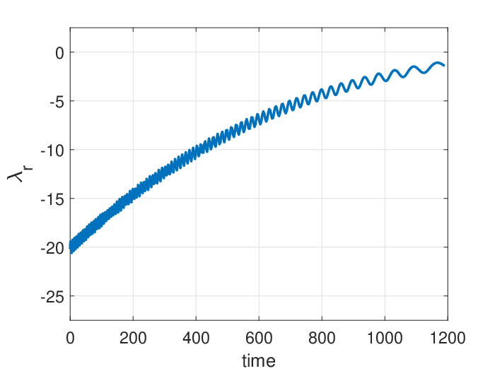
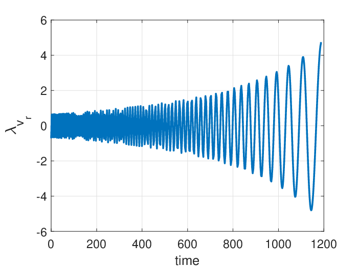
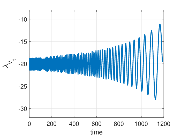
Thus, for example, the values of $\lambda_{r}$ in canonical-consistent units (see [7, 58]) has a range of about $2,000$ time units per distance units. By scaling down the cost function (time units) by a factor of $100$, the range of values of $\lambda_{r}$ was brought down roughly consistent with that of $r$ (of $6$ units, per (5.3)). As apparent from Fig. 8, the same scale factor generated a roughly balanced problem with respect to the other primal-dual pairs, namely, $(\theta,\lambda_{\theta})$, $(v_{r},\lambda_{v_{r}})$ and $(v_{t},\lambda_{v_{t}})$. Note also that, except for $\lambda_{\theta}$, the costates are highly oscillatory. Taken all together, i.e., grid density, oscillatory functions, condition numbers, scaling and balancing, it is clear why a low-thrust trajectory optimization problem is challenging.

Applying (48) to Problem $(O_{Xfer})$, it is straightforward to show that an optimal trajectory must satisfy the following necessary conditions:

That (78a) is satisfied is apparent from Fig. 8. The satisfaction of (78b) and (78c) over the primal-feasible solution of Fig. 7 is shown in Fig. 9.

References

- [1] I. M. Ross, “A Universal Birkhoff Theory for Fast Trajectory Optimization,” arXiv preprint, arXiv:2308.01400, 2023. https://arxiv.org/pdf/2308.01400.pdf
- [2] I. M. Ross, R. J. Proulx, C. F. Borges, “A Universal Birkhoff Pseudospectral Method for Solving Boundary Value Problems,” Applied Mathematics and Computation, Vol. 454, 128101, 2023.
- [3] L.-L Wang, M. D. Samson and X. Zhao, “A Well-Conditioned Collocation Method Using a Pseudospectral Integration Matrix,” SIAM Journal of Scientific Computaton, Vol. 36, No. 3, pp. A907-A929, 2014.
- [4] N. Koeppen, I. M. Ross, L. C. Wilcox and R. J. Proulx, “Fast Mesh Refinement in Pseudospectral Optimal Control,” Journal of Guidance, Control, and Dynamics, vol. 42 no. 4, pp. 711-722, 2018.
- [5] I. M. Ross and R. J. Proulx, “Further Results on Fast Birkhoff Pseudospectral Optimal Control Programming,” Journal of Guidance, Control, and Dynamics, vol. 42 no. 9, pp. 2086–2092, 2019.
- [6] I. M. Ross, “A Roadmap for Optimal Control: The Right Way to Commute,” Annals of the New York Academy of Sciences, 1065/1, 2005, 210–231.
- [7] I. M. Ross, A Primer on Pontryagin’s Principle in Optimal Control, Second Edition, Collegiate Publishers, San Francisco, CA, 2015.
- [8] Q. Gong, I. M. Ross, W. Kang and F. Fahroo, “On the Pseudospectral Covector Mapping Theorem for Nonlinear Optimal Control,” Proceedings of the 45th IEEE Conference on Decision and Control, 2006, pp. 2679-2686, doi: 10.1109/CDC.2006.377729.
- [9] I. M. Ross, “A Historical Introduction to the Covector Mapping Principle,” Advances in the Astronautical Sciences, Vol. 123, Univelt, San Diego, CA, 2006, pp. 1257–1278.
- [10] I. M. Ross and F. Fahroo, “A Perspective on Methods for Trajectory Optimization,” AIAA/AAS Astrodynamics Specialist Conference and Exhibit, 5-8 August, 2002, Monterey, CA. AIAA 2002-4727. https://doi.org/10.2514/6.2002-4727.
- [11] Fahroo, F., and Ross, I. M., “Costate estimation by a Legendre pseudospectral method,” AIAA Journal of Guidance, Control and Dynamics, Vol. 24, No. 2, pp. 270-277, 2001.
- [12] I. M. Ross and F. Fahroo, “Discrete Verification of Necessary Conditions for Switched Nonlinear Optimal Control Systems,” Proceedings of the American Control Conference, June 2004, Boston, MA.
- [13] F. Fahroo and I. M. Ross, “Advances in Pseudospectral Methods for Optimal Control,” AIAA Guidance, Navigation, and Control Conference, AIAA Paper 2008-7309, Honolulu, Hawaii, August 2008.
- [14] Q. Gong, I. M. Ross and F. Fahroo, “Costate Computation by a Chebyshev Pseudospectral Method,” Journal of Guidance, Control and Dynamics, Vol. 33, No. 2, pp. 623-628, 2010.
- [15] Q. Gong, I. M. Ross and F. Fahroo, “Pseudospectral Optimal Control On Arbitrary Grids,” AAS Astrodynamics Specialist Conference, AAS-09-405, 2009.
- [16] Q. Gong, I. M. Ross and F. Fahroo, “Spectral and Pseudospectral Optimal Control Over Arbitrary Grids,” Journal of Optimization Theory and Applications, vol. 169, no. 3, pp. 759-783, 2016.
- [17] I. M. Ross and M. Karpenko, “A Review of Pseudospectral Optimal Control: From Theory to Flight,” Annual Reviews in Control, Vol.36, No.2, pp.182–197, 2012.
- [18] B. Fornberg, A Practical Guide to Pseudospectral Methods. Cambridge University Press Cambridge, 1996.
- [19] J. Boyd, Chebyshev and Fourier Spectral Methods, Dover Publications, Inc., Minola, New York, 2001.
- [20] L. N. Trefethen, Spectral Methods in MATLAB. SIAM, Philadelphia, PA, 2000.
- [21] Hesthaven, J., Gottlieb, S., Gottlieb, D., Spectral Methods for Time-Dependent Problems Cambridge Monographs on Applied and Computational Mathematics, Cambridge University Press, Cambridge, UK, 2007.
- [22] J. S. Hesthaven, “Integration Preconditioning Of Pseudospectral Operators. I. Basic Linear Operators,” SIAM Journal of Numerical Analysis, Vol. 35, No. 4, pp. 1571-1593, 1998.
- [23] E. M. E. Elbarbary, “Integration Preconditioning Matrix for Ultraspherical Pseudospectral Operators,” SIAM Journal of Scientific Computaton, Vol. 28, No. 3, pp. 1186-1201, 2006.
- [24] L. N. Trefethen, Approximation Theory and Approximation Practice, SIAM, Philadelphia, PA, 2013.
- [25] I. Bogaert, Iteration-Free Computation of Gauss–Legendre Quadrature Nodes and Weights, SIAM J. Sci. Comput., 36/3 (2014), A1008-A1026.
- [26] L.-L. Wang, B.-Y. Guo, “Interpolation approximations based on Gauss-Lobatto-Legendre-Birkhoff quadrature,” Journal of Approximation Theory, Volume 161, Issue 1, 2009, Pages 142–173.
- [27] L. N. Trefethen, “Is Gauss Quadrature Better than Clenshaw-Curtis?” SIAM Review, Vol. 50, No. 1, pp. 67–87, 2008.
- [28] J. Waldvogel, “Fast Construction of the Fejér and Clenshaw-Curtis Quadrature Rules,” BIT Numerical Mathematics, 46, 2006, pp. 195–202.
- [29] F. Fahroo and I. M. Ross, “Convergence of the Costates Does Not Imply Convergence of the Control,” Journal of Guidance, Control and Dynamics, Vol. 31, No. 5, pp. 1492-1497, 2008.
- [30] Karpenko, M., Bhatt, S., Bedrossian, N., Ross, I. M., “Flight Implementation of Shortest-Time Maneuvers for Imaging Satellites,” Journal of Guidance, Control and Dynamics, Vol. 37, No. 4, pp. 1069–1079, 2014.
- [31] N. Bedrossian, S. Bhatt, W. Kang, I. M. Ross, “Zero Propellant Maneuver Guidance,” IEEE Control Systems Magazine, Vol. 29, Issue 5, October 2009, pp. 53-73.
- [32] N. Bedrossian, M. Karpenko, and S. Bhatt, “Overclock My Satellite: Sophisticated Algorithms Boost Satellite Performance on the Cheap,” IEEE Spectrum Magazine, Vol. 49, No. 11, 2012, pp. 54–62.
- [33] Q. Gong, F. Fahroo and I. M. Ross, “Spectral Algorithm for Pseudospectral Methods in Optimal Control,” Journal of Guidance, Control, and Dynamics, vol. 31 no. 3, pp. 460-471, 2008.
- [34] Q. Gong and I. M. Ross, “Autonomous Pseudospectral Knotting Methods for Space Mission Optimization,” Advances in the Astronatuical Sciences, Vol. 124, 2006, AAS 06-151, pp. 779–794.
- [35] I. M. Ross, “Enhancements to the DIDO Optimal Control Toolbox,” arXiv preprint, arXiv:2004.13112, 2020, https://arxiv.org/abs/2004.13112
- [36] I. M. Ross and F. Fahroo, “Pseudospectral Knotting Methods for Solving Optimal Control Problems,” Journal of Guidance, Control and Dynamics, Vol. 27, No. 3, pp. 397-405, 2004.
- [37] Ross, I. M., D’Souza, C. N., “Hybrid Optimal Control Framework for Mission Planning,” Journal of Guidance, Control and Dynamics, Vol. 28, No. 4, pp. 686–697, 2005.
- [38] I. M. Ross, F. Fahroo and J. Strizzi, “Adaptive Grids for Trajectory Optimization by Pseudospectral Methods,” AAS/AIAA Spaceflight Mechanics Conference, Paper No. AAS 03-142, Ponce, Puerto Rico, 9-13 February 2003.
- [39] I. M. Ross, Q. Gong and P. Sekhavat, “Low-Thrust, High-Accuracy Trajectory Optimization,” Journal of Guidance, Control and Dynamics, Vol. 30, No. 4, pp. 921–933, 2007.
- [40] I. M. Ross, Q. Gong and P. Sekhavat, “The Bellman Pseudospectral Method,” AIAA/AAS Astrodynamics Specialist Conference and Exhibit, Honolulu, Hawaii, AIAA-2008-6448, August 18-21, 2008.
- [41] F. Fahroo and I. M. Ross, “Pseudospectral Methods for Infinite-Horizon Nonlinear Optimal Control Problems,” Proceedings of the AIAA Guidance, Navigation and Control Conference, San Francisco, CA, August 15-18, 2005.
- [42] I. M. Ross, Q. Gong, F. Fahroo and W. Kang, “Practical stabilization through real-time optimal control,” Proceedings of the 2006 American Control Conference, Inst. of Electrical and Electronics Engineers, Piscataway, NJ, June 2006, pp. 14–16.
- [43] F. Fahroo and I. M. Ross, “Pseudospectral Methods for Infinite-Horizon Optimal Control Problems,” Journal of Guidance, Control and Dynamics, Vol. 31, No. 4, pp. 927–936, 2008.
- [44] T. A. Driscoll, N. Hale, and L. N. Trefethen, editors, Chebfun Guide, Pafnuty Publications, Oxford, 2014.
- [45] W. Chen, Z. Shao and L. T. Biegler, ”A Bilevel NLP Sensitivitybased Decomposition for Dynamic Optimization withMoving Finite Elements,” AIChE J., 2014, 60, 966–979.
- [46] W. Chen and L. T. Biegler, ”Nested Direct Transcription Optimization for Singular Optimal Control Problems,” AIChE J., 2016, 62, 3611–3627.
- [47] L. Ma, Z. Shao, W.Chen and Z. Song, ”Trajectory optimization for lunar soft landing with a Hamiltonian-based adaptive mesh refinement strategy,” Advances in Engineering Software Volume 100, October 2016, pp. 266–276.
- [48] I. M. Ross, “A Direct Shooting Method is Equivalent to An Indirect Method,” arXiv preprint (2020) arXiv:2003.02418.
- [49] H. Yan, Q. Gong, C. Park, I. M. Ross, and C. N. D’Souza, “High Accuracy Trajectory Optimization for a Trans-Earth Lunar Mission,” Journal of Guidance, Control and Dynamics, Vol. 34, No. 4, 2011, pp. 1219-1227.
- [50] S. Bhatt, N. Bedrossian, K. Longacre and L. Nguyen, “Optimal Propellant Maneuver Flight Demonstrations on ISS,” AIAA Guidance, Navigation, and Control Conference, August 19-22, 2013, Boston, MA. AIAA 2013-5027.
- [51] G. Minelli, M. Karpenko, I. M. Ross and J. Newman, “Autonomous Operations of Large-Scale Satellite Constellations and Ground Station Networks,” AAS/AIAA Astrodynamics Specialist Conference, August 20 - 24, 2017 Stevenson, WA. AAS-17-761
- [52] J. S. Meditch, “On the Problem of Optimal Thrust Programming for a Lunar Soft Landing,” IEEE Transactions on Automatic Control, AC-9, No. 4, pp. 477–484, 1964
- [53] Bryson, A. E., and Ho, Y.-C., Applied Optimal Control, Hemisphere, New York, 1975 (Revised Printing; original publication, 1969).
- [54] Dmitruk, A., Samylovskiy, I., “On the relation between two approaches to necessary optimality conditions in Problems with State Constraints,” J. Optim. Theory Appl., 173(2), 391–420 (2017)
- [55] A. Herman and B. A. Conway, “Direct Optimization Using Collocation Based on High-Order Gauss-Lobatto Quadrature Rules,” Journal of Guidance Control and Dynamics, Vol.39, No.3, 1996, pp.592–599.
- [56] B. A. Conway, “A Survey of Methods Available for the Numerical Optimization of Continuous Dynamic Systems,” Journal of Optimization Theory and Applications, Vol. 152, 2012, pp. 271–306.
- [57] E. Hairer, S. P. Nørsett, G. Wanner, Solving Ordinary Differential Equations I: Nonstiff Problems, Springer-Verlag Berlin Heidelberg, 1993.
- [58] I. M. Ross, Q. Gong, M. Karpenko and R. J. Proulx, “Scaling and Balancing for High-Performance Computation of Optimal Controls,” Journal of Guidance, Control and Dynamics, Vol. 41, No. 10, 2018, pp. 2086–2097.
- [59] Ross, I. M., “How to Find Minimum-Fuel Controllers,” AIAA Guidance, Navigation, and Control Conference and Exhibit, AIAA Paper 2004-5346, 2004.
- [60] N. Bedrossian, S. Bhatt, M. Lammers and L. Nguyen, “Zero Propellant Maneuver: Flight Results for 180∘ ISS Rotation,” 20th International Symposium on Space Flight Dynamics, September 24-28, 2007, Annapolis, MD, NASA/CP-2007-214158.
- [61] A. Fleming, P. Sekhavat, and I. M. Ross, “Minimum-Time Reorientation of a Rigid Body,” Journal of Guidance, Control, and Dynamics, Vol. 33, No.1, Jan-Feb 2010, pp. 160–170.
- [62] Karpenko, M., Lippman, T., Ross, I.M., Halverson, J.K., McClanahan, T., Barker, M., Mazarico, E., Besser, R., Dennehy, C.J., VanZwieten, T., and Wolf, A., “Fast Attitude Maneuvers for the Lunar Reconnaissance Orbiter,” 42nd Annual AAS Guidance & Control Conference, Jan. 31 to Feb. 6, 2019, Breckenridge, CO. Paper number: AAS 19-053.
- [63] Johnston, S. A., “Lunar Reconnaissance Orbiter gets an upgrade to capture new perspectives of the moon,” Universe Today, February 15, 2021, https://phys.org/news/2021-02-lunar-reconnaissance-orbiter-capture-perspectives.html
- [64] K. P. Bollino, High-Fidelity Real-Time Trajectory Optimization for Reusable Launch Vehicles, Ph.D. Dissertation, Naval Postgraduate School, Monterey, CA, Dec 2006.