Search for Galactic core-collapse supernovae in a decade of data taken with the IceCube Neutrino Observatory
Abstract
The IceCube Neutrino Observatory has been continuously taking data to search for s long neutrino bursts since 2007. Even if a Galactic core-collapse supernova is optically obscured or collapses to a black hole instead of exploding, it will be detectable via the MeV neutrino burst emitted during the collapse. We discuss a search for such events covering the time between April 17, 2008 and December 31, 2019. Considering the average data taking and analysis uptime of 91.7 % after all selection cuts, this is equivalent to 10.735 years of continuous data taking. In order to test the most conservative neutrino production scenario, the selection cuts were optimized for a model based on a 8.8 solar mass progenitor collapsing to an O-Ne-Mg core. Conservative assumptions on the effects of neutrino oscillations in the exploding star were made. The final selection cut was set to ensure that the probability to detect such a supernova within the Milky Way exceeds 99 %. No such neutrino burst was found in the data after performing a blind analysis. Hence, a 90 % C.L. upper limit on the rate of core-collapse supernovae out to distances of 25 kpc was determined to be 0.23/yr. For the more distant Magellanic Clouds, only high neutrino luminosity supernovae will be detectable by IceCube, unless external information on the burst time is available. We determined a model-independent limit by parameterizing the dependence on the neutrino luminosity and the energy spectrum.
Keywords:
supernova — neutrino — galacticI Introduction
Stars with masses larger than end their lives with the gravitational collapse of their core, followed by neutrino emission over a time scale of about 10 s and a shock-driven luminous explosion called a supernova. The expected volumetric rate of core-collapse supernovae (CCSNe) in the universe today is . By compiling results obtained with various methods, the rate of stellar collapses in the Milky Way, including those obscured in the optical waveband, was estimated to be per century (Rozwadowska et al. 2021). This corresponds to a mean time between CCSNe of years.
In spiral galaxies, observations indicate that CCSNe occur preferentially in the disc rather than the bulge component and therefore point to a relatively young progenitor population (Hakobyan et al. 2015). For this paper, we assume a Milky Way progenitor radial distribution model (Ahlers et al. 2009) that takes into account the geometry of the spiral arms (see Fig. 1).
In principle, it is simpler to estimate the CCSN rate in the Large and Small Magellanic Clouds at kpc and kpc distance, respectively, because our view is not obscured by the dense bulge of the Milky Way. The rate can be estimated by counting the number of observed supernova remnants (Vink 2020) and the use of an isotope measure to distinguish between core collapse and Type Ia supernovae (Maggi et al. 2016). In spite of the relatively small number of visible stars in the Large and Small Magellanic Clouds compared to the Milky Way, both add estimated CCSN rates of % to the Milky Way CCSN rate.
The detection of neutrinos from CCSNe is important as they reveal the conditions in the core region of the star at the time of the collapse. Neutrino experiments will also tell astronomers when and where they should point their telescopes, with several hours lead time (Abe et al. 2016; Brdar et al. 2018; Linzer & Scholberg 2019; Coleiro, A. et al. 2020).
The fraction of supernovae that will be missed in optical observations depends on how regularly the complete sky is monitored by astronomers and automated systems and on whether the supernova is obscured by dust. Infrared photons can penetrate dust in the inner region of the galaxy. Assuming an optimistic model of dust extinction and all-sky coverage by optical telescopes, 96 % of the supernovae in the Milky Way should be observable in the optical (Adams et al. 2013). For other dust models, this fraction may be lower, although dust extinction can be mitigated by automatic wide-angle infrared transient surveys (Moore & Kasliwal 2019). Predictions have also been obtained for the more distant Magellanic Clouds (Adams et al. 2013).
Massive stars may create a black hole that consumes the nascent supernova before the massive explosion. This is indicated by an observed deficit of supernova progenitors between 18 to 25 (Kochanek et al. 2008) and the merging of black holes observed by Advanced LIGO (Abbott et al. 2016) which were likely formed from failed supernovae. The fraction of supernovae that end up in black holes is not well known, however. A data-driven way to estimate the fraction is an optical search for progenitors that "suddenly disappear". An eleven year optical search (Neustadt et al. 2021) identified one clearly detected failed supernova candidate, corresponding to a 90 % confidence interval of for the fraction of core-collapses, resulting in failed or aborted supernovae. Failed supernovae would be identifiable by the fast drop of the neutrino emission and a longer lasting echo of higher energy neutrinos that may be observable by IceCube (Gullin et al. 2022).
It has been more than three decades since the first and only supernova has been observed by neutrino detection. On February 23, 1987, a burst of neutrinos with energies of a few tens of MeV emitted by the supernova SN1987A was recorded simultaneously by the Baksan (Alekseev et al. 1987), IMB (Bionta et al. 1987), and Kamiokande-II (Hirata et al. 1987; Hirata et al. 1988) detectors, a few hours before its optical counterpart was discovered. With just 24 neutrinos collected, important limits on the mass of the , its lifetime, its magnetic moment and the number of leptonic flavors were derived (Kotake et al. 2006).
The small observed number of events can be explained by the source distance ( kpc) and the limited active volumes of the detectors operational in 1987. As will be explained below, IceCube will register photons from interacting neutrinos if a supernova explodes at the Galactic Center. Such a high statistical accuracy will permit a study of detailed features of the neutrino emission that carries important information about the explosion dynamics and neutrino properties.
Several neutrino detectors have searched for nearby CCSNe in the last decades, e.g. water Cherenkov detectors (Ahrens et al. 2002; Ikeda et al. 2007; Abbasi et al. 2011; Aiello et al. 2022), scintillator detectors (Ambrosio et al. 2004; Novoseltsev et al. 2020; Agafonova et al. 2015; Aharmim et al. 2011; Rumleskie & Virtue 2020; Abe et al. 2022; Acero et al. 2021), lead-based detectors (Rosso 2021), as well as liquid noble gas neutrino (Abi et al. 2021) and dark matter detectors (Lang et al. 2016).
The most stringent experimental limits have been published by the Baksan Collaboration (Novoseltsev et al. 2022) over the period June 30, 1980 to June 30, 2021 with a livetime of 35.5 years. In the absence of a positive observation, they quote a rate of < 6.5 CCSNe per century within 20 kpc at 90 % C.L. The LVD Collaboration quotes a rate of < 8 CCSNe per century within 25 kpc at 90 % C.L. over the period 1992 to Jan 4, 2021 (Vigorito et al. 2021).
Both LVD and Baksan determined their limits referencing phenomenological models that have been parameterized to fit the 1987A observation, and thus correspond to massive progenitors. No neutrino oscillations were assumed by the Baksan Collaboration, whereas a normal neutrino hierarchy and MSW oscillations were taken into account in the LVD analysis.
The possibility to monitor supernovae in our Galaxy with high-energy neutrino telescopes was first pointed out by Pryor et al. 1988 and Halzen et al. 1996. A first search (Ahrens et al. 2002) based on 215 days of data taken in 1997 and 1998 with the still incomplete AMANDA detector demonstrated the feasibility of the approach. Since 2009, IceCube has been sending real-time messages to the Supernova Early Warning System SNEWS (Antonioli et al. 2004; Al Kharusi et al. 2021).
While the observation time of IceCube is shorter than that of Baksan and LVD, the large volume of IceCube provides sensitivity to a wide variety of models, ranging from the lightest CCSNe to heavy progenitors that end up in a black hole.
II Supernovae and Neutrinos
Neutrinos play a crucial role at all stages of the collapse of massive stars. In the initial phase of the collapse, the release of electron neutrinos by converting protons to neutrons accelerates the infall by removing the electron degeneracy pressure ("deleptonization phase"). The continuous accretion of outer layers of the progenitor star ("accretion phase") will eventually lead to the collapse and the formation of a dense and compact neutron star or a black hole. Matter bounces off this core ("core bounce") and emits a shock wave. The absorption of electron neutrinos and antineutrinos in the material surrounding the neutron star invigorates the shock so that the star is blown apart. Due to their small interaction cross section, only neutrinos and antineutrinos of all flavors carry away the gravitational binding energy of the compact and dense remnant ("cooling phase"). Subtleties in neutrino interactions, oscillations, and transport play a surprisingly large role. For a compilation on many aspects of supernova research see Alsabti & Murdin 2017.
The supernova core is sufficiently hot and dense to host a thermal population of neutrinos of all species that diffuse out and eventually reach the Earth. The neutrino thermal energy spectrum is expected to peak between 10 to 20 MeV, with and carrying lower energies as they are more strongly coupled to matter and evaporate later than and neutrinos. Neutrinos carry away 99 % of the gravitational binding energy released in the collapse, typically J, roughly equally distributed between the six neutrino and antineutrino species.
Flavor mixing effects can change the expected neutrino rates as well as the energy spectra compared to the original time-dependent flux, , and flux, . Deep inside the core, where the neutrino mean free path is comparable to the size of the proto-neutron star, flavor mixing may be ignored. Further away from the core, but within km from the center of the star, the density of neutrinos exceed that of electrons and the coherent scattering of neutrinos on each other can no longer be neglected (Lund & Kneller 2013). Such collective effects after the core bounce may lead to complex energy and time-dependent neutrino flavor conversions and the swapping of electron neutrinos with muon and tau neutrinos. At larger radii, the neutrino flavor conversion is driven by coherent scattering on electrons. Resonant enhancements for flavor conversion occur at densities around kg/m3 and kg/m3. Already in the vicinity of the supernova, the coherence of the mass eigenstates is lost, leading to wave packet separations at Earth of many meters (Kersten & Smirnov 2016).
The second and third generation neutrinos are mostly produced in the cooling phase and their fluxes are roughly equal. The mixing of the and fluxes is then given by
| (1) | |||||
| (2) |
The probabilities , depend on the mixing angle, collective effects, state transitions probabilities and matter densities (Mirizzi et al. 2016). If one neglects collective effects and assumes a static supernova matter profile with adiabatic state transitions, one obtains the simple relations
| (3) | |||||
| (4) |
for the normal neutrino mass hierarchy (NH) and inverted hierarchy (IH). When testing the effect of oscillations on models, we will use equations 3 and 4, as well as the no-oscillation case.
Oscillation effects can alter the detected signal as cross sections, fluxes, and energy spectra vary between flavors. While energies and fluxes are similar during the cooling phase, substantial differences in the early phase of neutrino emission may strongly modify the time-dependent flux. As the CCSN neutrino-induced hit rate in IceCube roughly rises with (Abbasi et al. 2011), it is particularly sensitive to oscillation-induced changes in the energy spectra. For each model we chose the oscillation scenario that leads to the lowest rate.
Finally, when neutrinos enter the material of the Earth, oscillations will occur that depend on the neutrino energy, the path length in matter and the material density. The resulting effect on the measured signal in IceCube will be discussed as part of the systematic uncertainties.
The initial phase of the neutrino emission is rather insensitive to the supernova progenitor mass. The total energy release in neutrinos depends directly on the mass of the neutron star (Lattimer & Prakash 2001) and only indirectly on the supernova progenitor mass. From 22 historic supernova remnants, Díaz-Rodríguez et al. 2021 find that the progenitor mass distribution is proportional to , with with a minimal progenitor mass of . Assuming these values, a substantial fraction, 10 % to 40 %, of all supernova progenitors, would have masses below 20 .
Various theory groups have performed extensive simulations of the supernova neutrino emission with ever increasing level of detail (e.g. Janka 2012; Burrows & Vartanyan 2021). Public codes exist that provide links between such simulations and simulations of neutrino detectors (Migenda et al. 2021; Baxter et al. 2022) and to quickly test physics signatures in current and future detectors (Scholberg et al. 2022; Malmenbeck & O’Sullivan 2019). While state-of-the-art calculations are performed in three-dimensional space, such calculations are very time consuming and only a few cover more than the first few hundred milliseconds until the explosion takes place (or not). For very low mass progenitors, and the early and late phases of neutrino emission, spherically symmetric simulations work reasonably well and will often lead to a neutrino-driven explosion in the simulation.
For the lowest expected signal we chose a s long simulation of a supernova from a 8.8 progenitor star that is triggered by electron-capture reactions and forms an O-Ne-Mg core (Hüdepohl et al. 2010), henceforth referred to as the “Hüdepohl model”. With a total emitted energy of J and a low mean neutrino energy of MeV, it represents a conservative lower limit for a supernova search.
The second choice is a 19 progenitor whose collapse was modeled in three dimensions up to 1.756 s after the core bounce (Bollig et al. 2021). Using an adaptive procedure, this simulation was stitched to a spherically symmetric simulation that continued into the cooling phase. The third model starts from a 27 model (Burrows & Vartanyan 2021) and follows the collapse and explosion with a cylindrically symmetric calculation that extends up to 4.5 s post-bounce.
On the high mass side, the gravitational collapse of stars exceeding will lead to a partial stellar explosion, while stars exceeding are not expected to explode at all (Smartt 2015; O’Connor 2017). In both cases, a black hole will develop (1) s after core bounce. At this point, the neutrino emission vanishes abruptly in non-rotating systems. For the analysis presented in this paper, we select a model assuming a 40 progenitor and a hard equation of state (Shen et al. 1998) for the neutron star (Sumiyoshi et al. 2007). This one-dimensional simulation of a non-rotating star ends in a black hole after 1.3 s. The model was also used in LVD’s result (Vigorito et al. 2021).
The time series of the neutrino emission differs substantially between the models. While it has been shown for one-dimensional simulations that most of the codes agree between various groups within 5 % (O’Connor et al. 2018), there are substantial differences when extending the calculations to more independent dimensions.
In the figures, we will refer to the models discussed in this section with the short forms "", "", "", and "". The two low (high) progenitor mass models yield the lowest rate in the no-oscillation (inverted hierarchy MSW) case.
To summarize, neutrinos are crucial during all stages of the stellar collapse and the explosion. They are, besides gravitational waves, the only means to obtain immediate information from the central regions of a dying star.
III The detection principle of IceCube
The IceCube Neutrino Observatory is a cubic-kilometer Cherenkov detector installed in the ice at the geographic South Pole (Aartsen et al. 2017) between depths of 1450 m and 2450 m. The detector was constructed from January 28, 2005 to December 18, 2010 by drilling holes into the Antarctic ice sheet in a hexagonal grid layout. Eighty-six cables (known as “strings”), instrumented with digital optical modules (DOMs) containing 10 inch hemispherical Hamamatsu R7081 photomultiplier tube (Abbasi et al. 2010), were lowered into the ice. Strings are spaced about 125 m apart and each contains 60 DOMs vertically separated by 17 m. Six central strings, with smaller string and sensor separations and equipped with 35 % higher quantum efficiency photosensors (HQE), are used in the DeepCore sub-array (Abbasi et al. 2012). The data used in this paper include the construction period where 2400, 3540, and 4740 DOMs became available to the data analysis during the first half of 2008, 2009 and 2010, respectively. The final detector consists of 5160 DOMs, of which 98.4 % are available to the analysis (Aartsen et al. 2017).
IceCube was designed to detect neutrinos with TeV energies and above. However, the neutrinos expected from CCSNe typically carry only MeV energies and only about 0.2 % of interactions within the detector volume will lead to at least one detected Cherenkov photon produced by secondary particles. Still, with a sufficient number of low-energy neutrinos interacting in the detector volume, a Galactic CCSN will produce a detectable correlated rise in the hit rate of all DOMs. Details of the detection method, the data acquisition system, and the physics capabilities can be found in Abbasi et al. 2011.
A dedicated pulse counter-based data acquisition is used to search for signatures of CCSNe. The search algorithm is based on count rates of individual DOMs stored in 1.67 ms time bins, which are downsampled to 500 ms intervals to perform various statistical analyses. An artificial deadtime of s was introduced to suppress time-correlated supra-Poissonian photomultiplier pulses at low temperatures that are most probably due to a temperature dependent radiative dissipation of energy deposited by radioactive decays in the glass (Meyer 2010; Heereman von Zuydtwyck 2015). This deadtime leads to an inefficiency that can be parameterized by , where denotes the excess rate per optical module from a CCSN (Abbasi et al. 2011). The resulting DOM background rate is below 300 Hz (see Fig. 2).
The stability of the DOM background rates is crucial for IceCube’s sensitivity to detect supernovae. By using automatic online procedures, faulty modules are excluded while acquiring the data. In the final 86-string configuration, 1.4 % of the 5160 modules were permanently excluded from the analysis and only modules with dynamically calculated background rates below 10 kHz were accepted. Operational modules were removed from the analysis if they exhibited either a variance much larger than the Poissonian expectation or a high skewness (Abbasi et al. 2011). Typically, only one or two DOMs are affected by the real time quality selection. In the very rare case where the number of qualified modules drops below a threshold of 100, the corresponding time periods were discarded as a safeguard to prevent sending false alerts to SNEWS.
By buffering the full photomultiplier raw data stream that is stored around candidate neutrino burst or external alerts, additional information can be retrieved (Heereman von Zuydtwyck 2015; Aartsen et al. 2017). For example, the average energy can be estimated from rare coincidences between adjacent DOMs (Fritz & Kappesser 2021) and the precision of the burst onset time can be improved.
Inverse beta decay, , dominates the interaction in water or ice (Abbasi et al. 2011). The signal hit rate per DOM for the inverse beta decay is given by
| (5) | |||||
where is the density of proton targets in ice, is the distance to the supernova, its neutrino luminosity, and is the normalized distribution depending on a shape parameter and on the average neutrino energy . denotes the energy of the positron emerging from the neutrino interaction. The effective volume for a single positron, , strongly varies with the photon absorption in the ice but shows little dependence on photon scattering. It is also directly proportional to the positron track length and thus to the positron energy (Abbasi et al. 2011).
IV Data preparation
The data used in this analysis cover the time between April 17, 2008, 03:43:54.16 UTC and December 31, 2019, 19:12:24.97 UTC (11.707 years) and were taken with four detector configurations of 40, 59, 79 and 86 strings, respectively. The data taking efficiency improved with time from 96 % in 2009 to 99.7 % in 2017. The average livetime was 98.4 % during this period.
The analysis requires that the detector works faultlessly in each of the million half-second time intervals studied. Therefore, additional measures are required to clean the data. Short runs (< 20 min), runs taken with calibration light sources, with an incomplete detector configuration, or containing data taking errors, were discarded. The total number of contributing DOMs was required to be larger than a minimum number, for example, 5060 DOMs out of a total of 5160 DOMs in case of the final IceCube detector configuration. We also required that the data acquisition for reconstructing muon tracks was working perfectly and that there was no known electromagnetic interference from external sources, such as radar surveys of the experimental site at the South Pole.
After rejecting such problematic data, the uptime available to the analysis ranged between 86.6 % and 96.8 %, with an average value of 91.7 %. The selected clean data, joined together, would correspond to 10.735 years of continuous data taking.
Atmospheric muons constitute a background to the search for CCSNe even though their energy when entering the ice sheet needs to be above 550 GeV to trigger the IceCube 8-fold majority trigger (Kelley 2015). Hence, hits from muon tracks that fail the trigger requirements are mostly found in the upper detector layers or clip the corners of the detector. Due to atmospheric density changes that are correlated to the air temperature, the muon rate shows a seasonal dependence and short term variations.
Because dust layers absorb light and many muons range out, the atmospheric muon-induced rate is depth-dependent and adds 3 Hz to 30 Hz to the Hz optical module background rate. This can be seen in Fig. 2, where the averaged count rate per DOM is shown as a function of time (blue points). The contribution from muons varies with the season. The red points show the rates after hits from identified muons were removed; the seasonal effect due to atmospheric muons is strongly reduced. The % reduction in rate is thought to be due to relieved stress in the refrozen ice near each DOM that decreases the effect of triboluminescence. It has been verified that the effect is not due to PMT aging (Aartsen et al. 2020a).
V Test statistic for the supernova search
The test statistic used to search for Galactic supernovae with IceCube is the significance proxy
| (6) |
where
| (7) |
is the most likely collective rate deviation of all rates from their running average. The average of the rates, , and the corresponding standard deviations are calculated from sliding 285 s time intervals before and after the central investigated time interval of 29.5 s duration. The factors account for quantum efficiency differences of the DOMs. Note that has the structure of a weighted average sum. The squared uncertainty on ,
| (8) |
is calculated from the data and thus accounts for non-Poissonian behavior in the background rates. In purely uncorrelated Poissonian processes, the significance should be centered at zero with unit width.
The calculation in the data acquisition was done in consecutive, non-overlapping 500 ms wide time intervals as well as in sliding 1.5, 4, 10 s time intervals overlapping by 500 ms. The sliding window approach introduces correlations and – picking the highest significance – distorts the Gaussian shape of the distribution by adding a high significance tail. We chose the 1.5 s time binning for all analyses as a conservative compromise among the models that were tested. As shown in Fig. 6, it covers the accretion phase with high neutrino intensity well.
The effect of muons on the significance proxy is much more pronounced than in the summed hits because muons create space and time-correlated hits. Therefore the optical sensor rates are no longer statistically independent and the central limit theorem is only partially fulfilled.
In fact, the vast majority of false positive alerts are due to a statistical clustering of atmospheric muon-induced hits: the rate of false alerts is cut by almost three orders of magnitude after removing hits associated with atmospheric muons.
In order to properly account for DOM rate variations, we correct for the muon contribution by a decorrelation method, which has been applied before in Aartsen et al. 2020b. We define a muon significance proxy by the relation
| (9) |
where all quantities are calculated on a per run basis. , the sum over all hits associated to a muon track, is taken as a measure of the atmospheric muon intensity.
A linear function is fit to the correlation between the supernova significance proxy and (see Fig. 3 for an example 8 hour run). A corrected significance proxy is calculated from the resulting offset and slope .
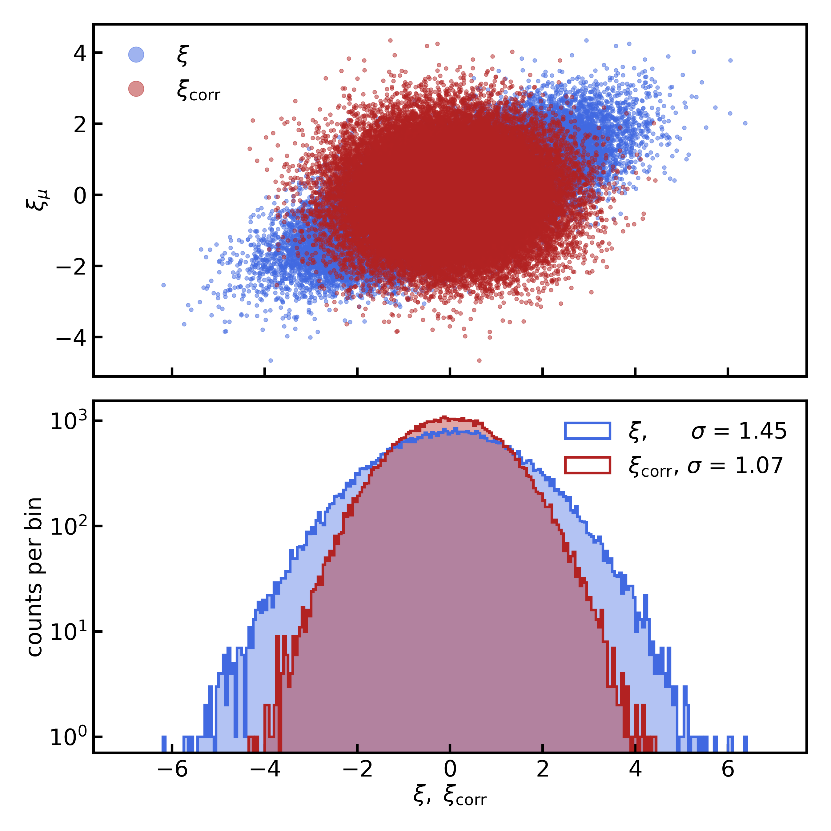
With the muon-corrected significance proxy defined, one can determine the false alert rate as function of the significance proxies and . Fig. 4 shows that the false alert rate can be reduced by a factor of for a significance proxy of 6, by applying the muon correction.
A slightly less effective atmospheric muon correction is already incorporated in the data acquisition by transmitting the subset of hits associated with IceCube’s simple majority triggers (Kelley 2015) to the supernova data acquisition system. The method has allowed us to lower the alert thresholds and reduce the number of false-positive alerts. For example, the SNEWS alert efficiency for potential supernovae in the Large Magellanic Cloud rose from 12 % to 82 % while meeting the SNEWS requirement that alerts are sent with a frequency of less than one alert per 14 days.
Lower threshold alerts are issued by the supernova data acquisition system at a rate of about 10 times per day. In this sense, the analysis discussed in this paper is not strictly "blind". However, the recalculation of the atmospheric muon-corrected data offline uses a much wider range of triggers and hits. We opted for an unblinding procedure to minimize the influence of prior knowledge by restricting the initial studies to a data set with .
VI Simulation
A GEANT4-based simulation of the interaction of individual supernova neutrinos in the ice and a computationally optimized tracking (Schwanekamp et al. 2022) of individual Cherenkov photons that can be run on graphical processing units was used to determine IceCube’s effective volume for supernova detection. Calibration measurements with light sources in the ice (Aartsen et al. 2017; Rongen et al. 2020) and a dust logger (Aartsen et al. 2013a) allow one to fit the depth-, position- and direction-dependent photon absorption and scattering lengths of the ice. The uncertainties in these measurements lead to a range of possible ice models. The model used in this paper incorporates position dependent scattering and absorption coefficients as well as an observed anisotropic attenuation effect aligned with the local flow of the ice (Rongen & Chirkin 2021; Abbasi et al. 2022).
Other important uncertainties arise from photon tracking in the presence of Mie scattering, optical module sensitivities, as well as from neutrino cross section uncertainties, though these are sizable only for interactions on 16O and 18O (Abbasi et al. 2011). The effective volume per optical module was determined by injecting positrons of 10 MeV energy with random directions and random positions inside a sphere with radius 250 m around every optical module along every string.
Fig. 5 shows the energy-independent quantity , which was determined from the fraction of positrons that generated photoelectrons at the cathode surface as function of depth. The higher quantum efficiency of the photomultipliers in the high density DeepCore sub-detector, installed in two ice regions below and above the main dust layer, is apparent. The effective volume scales linearly with the optical module sensitivities.
While a lot of effort has gone into in-situ calibrations of the ice properties (Aartsen et al. 2013b; Abbasi et al. 2022), uncertainties remain. The ice density is known to better than 0.2 %. The uncertainties on the scattering length, , and absorption length, , are presently estimated at 5 % each (Abbasi et al. 2023). Fig. 7 shows the result of studies with Monte Carlo samples of generated positrons each, where was varied within %. A quantitative evaluation shows a strong correlation between the effective volume uncertainty and the change in absorption length with for IceCube (DeepCore). The correlation with the scattering length, on the other hand, is very small: for IceCube (DeepCore). The color bands in Fig. 7 reflect the 5 % absorption coefficient uncertainty for IceCube and DeepCore. The result published in (Abbasi et al. 2011) is compatible with the new determination based on a much improved understanding of the ice properties.
Ice properties are not the only source of detector-related uncertainties (see Table 1). For example, the absolute DOM efficiency in-situ is presently known to 10 %. In addition, there are uncertainties on the cross sections. Neutrino interactions with oxygen are poorly known; however, they only play a role at neutrino energies beyond 20 MeV (see Tab. 1). Their contributions for 8.8 progenitor (Hüdepohl et al. 2010) and black hole forming (Sumiyoshi et al. 2007) models are estimated to be 1 % and 14 %, respectively.
We also studied potential uncertainties due to neutrino oscillations in the Earth matter. These become relevant when comparing the results of detectors at locations with different neutrino path lengths in the Earth or when the supernova position is unknown. The effect on the observed IceCube rate was studied as function of energy and incoming direction. The range of uncertainty for the low 8.8 model is given in Table 1. The uncertainty decreases once the position of the supernova is known.
| Source of | estimated relative |
|---|---|
| systematic uncertainty | uncertainty [%] |
| rate deviation in sliding average window | 1.6 |
| ice density as function of depth | 0.2 |
| mean track length in ice | 5 |
| ice properties | [-3.6, 4.1] |
| DOM efficiency | |
| artificial dead time | 3 |
| cross sections (, , scattering) | < 1, < 1, 0.2 |
| angle-dependent Earth oscillation | [-0.2,4.9] |
Since simulating events with the GEANT4-based Monte Carlo is computationally expensive, we calibrated a parameterized simulation program with these results. The fast Monte Carlo provides access to a large number of supernova models using time-dependent tables of luminosities, average neutrino energies and spectral shape parameters. The simulation also incorporates various oscillation mechanisms and is capable of injecting signal events into the data stream. One can do without a detailed time-dependent noise and atmospheric muon simulation by using random data sampled over the data taking period.
Fig. 8 shows the significance proxy versus the distance for the four selected models. The CCSN distances were simulated to follow the progenitor distribution of Ahlers et al. 2009.

Fig. 9 shows the probability densities as function of in our Galaxy within 25 kpc and the Magellanic Clouds for the four models. The data are shown in the range . The effect of varying the assumed progenitor distance distribution is small (not shown).
Large uncertainties in the modeling of supernovae may remain even if an optical counterpart can be studied in detail. This is also true for the complex neutrino oscillation effects in the core of the developing supernova. Addressing these uncertainties goes beyond the scope of this paper.
VII Results on the Galactic CCSN search
From the probability density distributions in Fig. 9, including systematic uncertainties, we determined the potential signal region by requiring that 99 % of all CCSNe in our galaxy for the lightest progenitor studied in this analysis should be detected. For the complete IceCube detector, including the systematic effects in Table 1, the signal region is defined by . The data with were then unblinded and the subthreshold range and the signal range were investigated. We present in Fig. 10 the accumulated result using the the distribution. No event in the signal region is found. However, two events entered the subthreshold range, with and . Both events are close in time to failed runs. The estimated background assuming a power law distribution (Pareto 1964) in the blinded region amounts to events.
A 90 % C.L.upper limit was determined using the Feldman-Cousins method (Feldman & Cousins 1998), conservatively assuming no background and the equivalent of 10.735 years of continuous data taking. The limit
| (10) |
covers supernovae within 25 kpc distance, including those that are optically hidden or failed to explode.
As can be seen from Fig. 9, only high neutrino luminosity supernovae can be detected in the Small and Large Magellanic Clouds by IceCube alone. However, the situation improves if the burst time is known from external sources, such as other neutrino detectors, a gravitational wave detector, or an astronomical observation with electromagnetic waves. Unfortunately, the progenitor mass does not uniquely define the observable neutrino flux. We therefore choose to define a progenitor mass-independent measure that is proportional to the observed rate of hits in IceCube. It scales roughly with the third power of the neutrino energy and depends on the spectral shape that is defined in this analysis by the numerical parameter (Keil et al. 2003). We introduce the quantity
| (11) |
to set a lower limit for the observation of supernovae in the Magellanic Clouds that fulfill the condition MeV3. Among the models investigated in this paper, the requirement is satisfied for the 27 model (Burrows & Vartanyan 2021) and the black hole model (Sumiyoshi et al. 2007).
The search discussed in this paper was optimized for the random occurrence of a supernova in the Milky Way and its dwarf galaxy companions. In principle, the sensitivity would be higher for phenomena that occur at fixed frequencies, such as a “neutrino pulsar” (Mushtukov et al. 2018). Checking the data quality is another reason to study the data set in the frequency domain. Lomb-Scargle periodograms were used to investigate the data sample in frequency space, up to Nyquist frequencies of 1 Hz (Fritz & Kappesser 2021; Fritz 2022). With the exception of a signature of the diurnal seasonal oscillation of the muon rate and artifacts from the run transitions and alias effects at high frequency, no significant signal was found.
VIII Conclusions
A search for neutrinos from core-collapse supernovae in the Milky Way and dwarf galaxy companions using IceCube data taken between April 17, 2008 and December 31, 2019 was performed. The period covers the equivalent of 10.735 years of uninterrupted data taking. With the cuts defined in this analysis and for distances smaller than 25 kpc, IceCube has the sensitivity to detect 99 % of all Galactic core-collapse supernovae with neutrino fluxes equal to or higher than that of the conservative progenitor model. No candidate event was found and a 90 % C.L. upper limit on the rate of core-collapse supernovae out to distances of 25 kpc was determined to be 0.23/yr. This limit can be extended to the Magellanic Clouds for models that fulfill the condition MeV3, with the progenitor mass independent measure defined in section VII.
As part of the approved IceCube Upgrade, multi-PMT modules (Abbasi et al. 2021) will be deployed and low-noise wavelength-shifting sensors (Bastian-Querner et al. 2022) will be tested. They have the potential to increase the distance reach (Lozano Mariscal et al. 2021) and will substantially improve the spectral sensitivity.
Acknowledgements
The IceCube collaboration acknowledges the significant contribution to this manuscript from Alexander Fritz. The authors gratefully acknowledge the support from the following gencies:
USA – U.S. National Science Foundation-Office of Polar Programs, U.S. National Science Foundation-Physics Division, U.S. National Science Foundation-EPSCoR, Wisconsin Alumni Research Foundation, Center for High Throughput Computing (CHTC) at the University of Wisconsin–Madison, Open Science Grid (OSG), Advanced Cyberinfrastructure Coordination Ecosystem: Services & Support (ACCESS), Frontera computing project at the Texas Advanced Computing Center, U.S. Department of Energy-National Energy Research Scientific Computing Center, Particle astrophysics research computing center at the University of Maryland, Institute for Cyber-Enabled Research at Michigan State University, and Astroparticle physics computational facility at Marquette University; Belgium – Funds for Scientific Research (FRS-FNRS and FWO), FWO Odysseus and Big Science programmes, and Belgian Federal Science Policy Office (Belspo); Germany – Bundesministerium für Bildung und Forschung (BMBF), Deutsche Forschungsgemeinschaft (DFG), Helmholtz Alliance for Astroparticle Physics (HAP), Initiative and Networking Fund of the Helmholtz Association, Deutsches Elektronen Synchrotron (DESY), and High Performance Computing cluster of the RWTH Aachen; Sweden – Swedish Research Council, Swedish Polar Research Secretariat, Swedish National Infrastructure for Computing (SNIC), and Knut and Alice Wallenberg Foundation; European Union – EGI Advanced Computing for research; Australia – Australian Research Council; Canada – Natural Sciences and Engineering Research Council of Canada, Calcul Québec, Compute Ontario, Canada Foundation for Innovation, WestGrid, and Compute Canada; Denmark – Villum Fonden, Carlsberg Foundation, and European Commission; New Zealand – Marsden Fund; Japan – Japan Society for Promotion of Science (JSPS) and Institute for Global Prominent Research (IGPR) of Chiba University; Korea – National Research Foundation of Korea (NRF); Switzerland – Swiss National Science Foundation (SNSF); United Kingdom – Department of Physics, University of Oxford.
References
- Aartsen et al. (2013a) Aartsen, M. G., et al. 2013a, Journal of Glaciology, 59, 1117–1128, doi: 10.3189/2013JoG13J068
- Aartsen et al. (2013b) —. 2013b, Nucl. Instrum. Meth. A, 711, 73, doi: 10.1016/j.nima.2013.01.054
- Aartsen et al. (2017) —. 2017, JINST, 12, P03012, doi: 10.1088/1748-0221/12/03/P03012
- Aartsen et al. (2020a) —. 2020a, JINST, 15, P06032, doi: 10.1088/1748-0221/15/06/P06032
- Aartsen et al. (2020b) —. 2020b, Astrophys. J., 890, 111, doi: 10.3847/1538-4357/ab564b
- Abbasi et al. (2010) Abbasi, R., et al. 2010, Nucl. Instrum. Meth. A, 618, 139, doi: 10.1016/j.nima.2010.03.102
- Abbasi et al. (2011) —. 2011, Astron. Astrophys., 535, A109, doi: 10.1051/0004-6361/201117810e
- Abbasi et al. (2012) —. 2012, Astropart. Phys., 35, 615, doi: 10.1016/j.astropartphys.2012.01.004
- Abbasi et al. (2021) —. 2021, PoS, ICRC2021, 1070, doi: 10.22323/1.395.1070
- Abbasi et al. (2022) —. 2022, The Cryosphere Discussions, 2022, 1, doi: 10.5194/tc-2022-174
- Abbasi et al. (2023) —. 2023, Measurement of Atmospheric Neutrino Mixing with Improved IceCube DeepCore Calibration and Data Processing. https://arxiv.org/abs/2304.12236
- Abbott et al. (2016) Abbott, B. P., et al. 2016, Phys. Rev. Lett., 116, 061102, doi: 10.1103/PhysRevLett.116.061102
- Abe et al. (2016) Abe, K., et al. 2016, Astropart. Phys., 81, 39, doi: 10.1016/j.astropartphys.2016.04.003
- Abe et al. (2022) Abe, S., et al. 2022, Astrophys. J., 934, 85, doi: 10.3847/1538-4357/ac7a3f
- Abi et al. (2021) Abi, B., et al. 2021, Eur. Phys. J. C, 81, doi: 10.1140/epjc/s10052-021-09166-w
- Acero et al. (2021) Acero, M. A., et al. 2021, Phys. Rev. D, 104, 063024, doi: 10.1103/PhysRevD.104.063024
- Adams et al. (2013) Adams, S. M., Kochanek, C. S., Beacom, J. F., Vagins, M. R., & Stanek, K. Z. 2013, Astrophys. J., 778, 164, doi: 10.1088/0004-637X/778/2/164
- Agafonova et al. (2015) Agafonova, N. Y., et al. 2015, Astrophys. J., 802, 47, doi: 10.1088/0004-637X/802/1/47
- Aharmim et al. (2011) Aharmim, B., et al. 2011, Astrophys. J., 728, 83, doi: 10.1088/0004-637X/728/2/83
- Ahlers et al. (2009) Ahlers, M., Mertsch, P., & Sarkar, S. 2009, Phys. Rev. D, 80, 123017, doi: 10.1103/PhysRevD.80.123017
- Ahrens et al. (2002) Ahrens, J., et al. 2002, Astropart. Phys., 16, 345, doi: 10.1016/S0927-6505(01)00154-2
- Aiello et al. (2022) Aiello, S., et al. 2022, Eur. Phys. J. C, 82, 317, doi: 10.1140/epjc/s10052-022-10137-y
- Al Kharusi et al. (2021) Al Kharusi, S., et al. 2021, New J. Phys., 23, 031201, doi: 10.1088/1367-2630/abde33
- Alekseev et al. (1987) Alekseev, E. N., Alekseeva, L. N., Volchenko, V. I., & Krivosheina, I. V. 1987, JETP Lett., 45, 589
- Alsabti & Murdin (2017) Alsabti, A. W., & Murdin, P., eds. 2017, Handbook of Supernovae (Springer International Publishing), doi: 10.1007/978-3-319-20794-0
- Ambrosio et al. (2004) Ambrosio, M., et al. 2004, Eur. Phys. J. C, 37, 265, doi: 10.1140/epjc/s2004-01981-3
- Antonioli et al. (2004) Antonioli, P., et al. 2004, New J. Phys., 6, 114, doi: 10.1088/1367-2630/6/1/114
- Bastian-Querner et al. (2022) Bastian-Querner, B., et al. 2022, Sensors, 22, 1385, doi: 10.3390/s22041385
- Baxter et al. (2022) Baxter, A. L., et al. 2022, Astrophys. J, 925, 107, doi: 10.3847/1538-4357/ac350f
- Bionta et al. (1987) Bionta, R. M., et al. 1987, Phys. Rev. Lett., 58, 1494, doi: 10.1103/PhysRevLett.58.1494
- Bollig et al. (2021) Bollig, R., et al. 2021, Astrophys. J., 915, 28, doi: 10.3847/1538-4357/abf82e
- Brdar et al. (2018) Brdar, V., Lindner, M., & Xu, X.-J. 2018, JCAP, 2018, 025, doi: 10.1088/1475-7516/2018/04/025
- Burrows & Vartanyan (2021) Burrows, A., & Vartanyan, D. 2021, Nature, 589, 29, doi: 10.1038/s41586-020-03059-w
- Coleiro, A. et al. (2020) Coleiro, A., Molla, M. Colomer, Dornic, D., Lincetto, M., & Kulikovskiy, V. 2020, Eur. Phys. J. C, 80, 856, doi: 10.1140/epjc/s10052-020-8407-7
- Díaz-Rodríguez et al. (2021) Díaz-Rodríguez, M., Murphy, J. W., Williams, B. F., Dalcanton, J. J., & Dolphin, A. E. 2021, Monthly Notices of the Royal Astronomical Society, 506, 781, doi: 10.1093/mnras/stab1800
- Feldman & Cousins (1998) Feldman, G. J., & Cousins, R. D. 1998, Phys. Rev. D, 57, 3873, doi: 10.1103/physrevd.57.3873
- Fritz (2022) Fritz, A. 2022, PhD thesis, Mainz U., doi: 10.25358/openscience-7825
- Fritz & Kappesser (2021) Fritz, A., & Kappesser, D. 2021. https://arxiv.org/abs/2108.05138
- Gullin et al. (2022) Gullin, S., O’Connor, E. P., Wang, J.-S., & Tseng, J. 2022, Astrophys. J., 926, 212, doi: 10.3847/1538-4357/ac4420
- Hakobyan et al. (2015) Hakobyan, A. A., Karapetyan, A. G., Barkhudaryan, L. V., et al. 2015, Monthly Notices of the Royal Astronomical Society, 456, 2848, doi: 10.1093/mnras/stv2853
- Halzen et al. (1996) Halzen, F., Jacobsen, J. E., & Zas, E. 1996, Phys. Rev. D, 53, 7359, doi: 10.1103/PhysRevD.53.7359
- Heereman von Zuydtwyck (2015) Heereman von Zuydtwyck, D. F. 2015, PhD thesis, U. Brussels (main). https://difusion.ulb.ac.be/vufind/Record/ULB-DIPOT:oai:dipot.ulb.ac.be:2013/209179/Holdings
- Hirata et al. (1987) Hirata, K., et al. 1987, Phys. Rev. Lett., 58, 1490, doi: 10.1103/PhysRevLett.58.1490
- Hirata et al. (1988) Hirata, K. S., et al. 1988, Phys. Rev. D, 38, 448, doi: 10.1103/PhysRevD.38.448
- Hüdepohl et al. (2010) Hüdepohl, L., Müller, B., Janka, H. T., Marek, A., & Raffelt, G. G. 2010, Phys. Rev. Lett., 104, 251101, doi: 10.1103/PhysRevLett.104.251101
- Ikeda et al. (2007) Ikeda, M., et al. 2007, Astrophys. J., 669, 519, doi: 10.1086/521547
- Janka (2012) Janka, H.-T. 2012, Annu. Rev. Nucl. Part. Sci., 62, 407, doi: 10.1146/annurev-nucl-102711-094901
- Keil et al. (2003) Keil, M. T., Raffelt, G. G., & Janka, H.-T. 2003, Astrophys. J., 590, 971, doi: 10.1086/375130
- Kelley (2015) Kelley, J. L. 2015, AIP Conf. Proc., 1630, 154, doi: 10.1063/1.4902795
- Kersten & Smirnov (2016) Kersten, J., & Smirnov, A. Y. 2016, Eur. Phys. J. C, 76, 339, doi: 10.1140/epjc/s10052-016-4187-5
- Kochanek et al. (2008) Kochanek, C. S., Beacom, J. F., Kistler, M. D., et al. 2008, Astrophys. J., 684, 1336, doi: 10.1086/590053
- Kotake et al. (2006) Kotake, K., Sato, K., & Takahashi, K. 2006, Rept. Prog. Phys., 69, 971, doi: 10.1088/0034-4885/69/4/R03
- Lang et al. (2016) Lang, R. F., McCabe, C., Reichard, S., Selvi, M., & Tamborra, I. 2016, Phys. Rev. D, 94, doi: 10.1103/physrevd.94.103009
- Lattimer & Prakash (2001) Lattimer, J. M., & Prakash, M. 2001, Astrophys. J., 550, 426, doi: 10.1086/319702
- Linzer & Scholberg (2019) Linzer, N. B., & Scholberg, K. 2019, Phys. Rev. D, 100, 103005, doi: 10.1103/PhysRevD.100.103005
- Lozano Mariscal et al. (2021) Lozano Mariscal, C. J., et al. 2021, Eur. Phys. J. C, 81, 1058, doi: 10.1140/epjc/s10052-021-09809-y
- Lund & Kneller (2013) Lund, T., & Kneller, J. P. 2013, Phys. Rev. D, 88, 023008, doi: 10.1103/PhysRevD.88.023008
- Maggi et al. (2016) Maggi, P., et al. 2016, Astron. Astrophys., 585, A162, doi: 10.1051/0004-6361/201526932
- Malmenbeck & O’Sullivan (2019) Malmenbeck, F., & O’Sullivan, E. 2019, in 36th International Cosmic Ray Conference. https://arxiv.org/abs/1909.00886
- Meyer (2010) Meyer, H. O. 2010, Europhysics Letters, 89, 58001, doi: 10.1209/0295-5075/89/58001
- Migenda et al. (2021) Migenda, J., Cartwright, S., Kneale, L., et al. 2021, J. Open Source Softw., 6, 2877, doi: 10.21105/joss.02877
- Mirizzi et al. (2016) Mirizzi, A., et al. 2016, La Rivista del Nuovo Cimento, 39, 1–112, doi: 10.1393/ncr/i2016-10120-8
- Moore & Kasliwal (2019) Moore, A. M., & Kasliwal, M. M. 2019, Nature Astronomy, 3, 109, doi: 10.1038/s41550-018-0675-x
- Mushtukov et al. (2018) Mushtukov, A. A., et al. 2018, Monthly Notices of the Royal Astronomical Society, 474, 5425, doi: 10.1093/mnras/stx2905
- Neustadt et al. (2021) Neustadt, J. M., et al. 2021, Monthly Notices of the Royal Astronomical Society, 508, 516, doi: 10.1093/mnras/stab2605
- Novoseltsev et al. (2020) Novoseltsev, Y. F., et al. 2020, Astropart. Phys., 117, 102404, doi: 10.1016/j.astropartphys.2019.102404
- Novoseltsev et al. (2022) —. 2022, J. Exp. Theor. Phys., 134, 390, doi: 10.1134/S1063776122040082
- O’Connor (2017) O’Connor, E. 2017, The Core-Collapse Supernova-Black Hole Connection, ed. A. W. Alsabti & P. Murdin (Springer International Publishing), doi: 10.1007/978-3-319-20794-0_129-1
- O’Connor et al. (2018) O’Connor, E., et al. 2018, J. Phys. G, 45, 104001, doi: 10.1088/1361-6471/aadeae
- Pareto (1964) Pareto, V. 1964, Cours d’Économie Politique: Nouvelle édition par G.-H. Bousquet et G. Busino, 299–345
- Pryor et al. (1988) Pryor, C., Roos, C. E., & Webster, M. S. 1988, Astrophys. J., 329, 335, doi: 10.1086/166381
- Rongen et al. (2020) Rongen, M., Bay, R. C., & Blot, S. 2020, The Cryosphere, 14, 2537, doi: 10.5194/tc-14-2537-2020
- Rongen & Chirkin (2021) Rongen, M., & Chirkin, D. 2021, Journal of Instrumentation, 16, C09014, doi: 10.1088/1748-0221/16/09/C09014
- Rosso (2021) Rosso, A. G. 2021, JCAP, 2021, 046, doi: 10.1088/1475-7516/2021/06/046
- Rozwadowska et al. (2021) Rozwadowska, K., Vissani, F., & Cappellaro, E. 2021, New Astron., 83, 101498, doi: 10.1016/j.newast.2020.101498
- Rumleskie & Virtue (2020) Rumleskie, J., & Virtue, C. 2020, J. Phys. Conf. Ser., 1342, 012135, doi: 10.1088/1742-6596/1342/1/012135
- Scholberg et al. (2022) Scholberg, K., et al. 2022, SNOwGLoBES, https://github.com/SNOwGLoBES/snowglobes, GitHub
- Schwanekamp et al. (2022) Schwanekamp, H., et al. 2022, Comput. Softw. Big Sci., 6, 4, doi: 10.1007/s41781-022-00080-8
- Shen et al. (1998) Shen, H., Toki, H., Oyamatsu, K., & Sumiyoshi, K. 1998, Nuclear Physics A, 637, 435, doi: https://doi.org/10.1016/S0375-9474(98)00236-X
- Smartt (2015) Smartt, S. J. 2015, Publications of the Astronomical Society of Australia, 32, doi: 10.1017/pasa.2015.17
- Sumiyoshi et al. (2007) Sumiyoshi, K., Yamada, S., & Suzuki, H. 2007, Astrophys. J., 667, 382, doi: 10.1086/520876
- Vigorito et al. (2021) Vigorito, C. F., Bruno, G., Fulgione, W., & Molinario, A. 2021, PoS, ICRC2021, 1111, doi: 10.22323/1.395.1111
- Vink (2020) Vink, J. 2020, Physics and Evolution of Supernova Remnants, doi: 10.1007/978-3-030-55231-2