Optimal design of plane elastic membranes using the convexified Föppl’s model

The out-of-plane equilibrium of a planar membrane occupying a domain $\Omega\subset\mathbb{R}^{2}$ and clamped on its boundary ${\partial\Omega}$ can be written down as follows:

The unknown function $w:\Omega\to\mathbb{R}$ represents the membrane’s out-of-plane displacement (normal displacement or deflection, for short). It must satisfy the Dirichlet boundary condition $w=0$ on ${\partial\Omega}$. The applied load $f:\Omega\to\mathbb{R}$ acts perpendicularly to the plane. The in-plane stress in the membrane is modeled by a function $\sigma:\Omega\to{\mathcal{S}^{2\times 2}_{+}}$, valued in symmetric positive semi-definite matrices. The positivity condition enforces that the membrane is capable of withstanding tensile stresses only, thus excluding the compressive ones. In the simplest variant, one assumes that the stress does not depend on the load $f$, and that it is homogeneous and hydrostatic, i.e. $\sigma=s\,\mathrm{I}_{2}$ where $s>0$ is a positive constant, $\mathrm{I}_{2}$ is the $2\times 2$ identity matrix. Such a setting is justified if on the boundary ${\partial\Omega}$ the membrane is subject to a pre-stress exerted by a normal traction of intensity $s$ that is sufficiently large, see e.g. [31, Section 5.10]. By taking such $\sigma$ we recast the most basic membrane model to be found as the leading example of a linear boundary value problem in some of the classical books on mathematical physics [34]. Indeed, in this case the equilibrium equation (1.1) reduces to the Poisson equation $-s\,\triangle w=f$.

In the sequel of this subsection $\Omega$ will not represent the membrane itself, but rather the design domain in which the material is to be optimally distributed. When addressing the issue of optimal design of membranes one cannot ignore the fact that equation (1.1) governs yet another problem in physics: the one of planar stationary heat flow where, in turn, $w$ is temperature, $f$ is the heat source/sink, and in place of $\sigma$ one has the conductivity tensor $A:\Omega\to{\mathcal{S}^{2\times 2}_{+}}$ that characterizes the 2D conductor. Meanwhile, optimization of conductors is a classical topic. Various settings are possible; in majority of them we essentially look for the field $A$ that satisfies some constraint on the amount of the material and that minimizes the adequately defined energy. If we assume that $A=a\mathbbm{1}_{\omega}\mathrm{I}_{2}$, where $a>0$ is a fixed positive constant and $\mathbbm{1}_{\omega}$ is the characteristic function of a subdomain $\omega\subset\Omega$ satisfying the constraint on the volume ${\left\lvert\omega\right\rvert}\leq V_{0}<{\left\lvert\Omega\right\rvert}$, then we find ourselves in the framework of shape optimization [70, 61, 27]. In general, optimal shapes do not exists, and it is when the relaxation by homogenization method [53, 2] intervenes. A different approach consists in finding an optimal mass or material distribution [20, 23] being a positive measure $\mu\in{\mathcal{M}}_{+}({\overline{\Omega}})$ satisfying $\mu({\overline{\Omega}})\leq V_{0}$, which generates a matrix valued measure $\mathcal{A}=(a\mathrm{I}_{2})\mu\in{\mathcal{M}}({\overline{\Omega}};{\mathcal{S}^{2\times 2}_{+}})$. The free material design [20, 58] is a variant of the latter formulation, when an arbitrary anisotropic measure $\mathcal{A}\in{\mathcal{M}}({\overline{\Omega}};{\mathcal{S}^{2\times 2}_{+}})$ is admissible provided that $\int_{\overline{\Omega}}{\mathrm{Tr}}\,\mathcal{A}\leq V_{0}$ . Most of the work cited above concerns not only the optimal design in conductivity, but also 2D or 3D linear elasticity. Then, one usually minimizes the compliance, defined as the work of the load on the induced displacements; cf. [18] for the free material design problem in this context.

Regardless of the aforementioned mathematical reminiscence between the statics of a membrane and the stationary heat flow, the far reaching advances in the optimal design of conductors quoted above cannot be transferred to optimizing membranes. We must mind that, unlike the conductivity tensor $A:\Omega\to{\mathcal{S}^{2\times 2}_{+}}$, the stress tensor $\sigma:\Omega\to{\mathcal{S}^{2\times 2}_{+}}$ is not a material property that we can control freely point by point as we see fit. Since $\sigma$ is an in-plane stress, it must meet the in-plane equilibrium equation:

where the zero right hand side reflects the lack of an in-plane loading. In the paper [17], co-written by the present author, a formulation of optimal design of membranes is proposed by adding (1.2) as a constraint in the free material design formulation. Formally, one seeks a stress tensor $\sigma:\Omega\to{\mathcal{S}^{2\times 2}_{+}}$ satisfying $\int_{\Omega}{\mathrm{Tr}}\,\sigma\,dx\leq V_{0}$ and $-{\mathrm{Div}}\,\sigma=0$ in $\Omega$; the target is to minimize the membrane’s compliance. Assuming that for a given $\sigma$ the equation (1.1) admits a solution $w_{\sigma}$, the compliance can be defined as $\int_{\Omega}w_{\sigma}f\,dx$. To the best of the present author’s knowledge, such an optimization setting is entirely new in the literature, and so are the optimal designs obtained in [17]. In fact, it is the author’s belief that the topic of optimizing membranes as mechanical systems is rather left out overall.

It is only fair to point out a drawback of the paper [17]: the premise for the optimal design formulation is heuristic from the mechanical point of view. Above all, it is not a priori justified to control the stress $\sigma$ in the whole domain ${\overline{\Omega}}$ as if it was a design variable – physically, we cannot impose the stress anywhere but on the boundary ${\partial\Omega}$. In the interior $\Omega$ the stress $\sigma$ should be induced via a constitutive law of elasticity, as a response to strain. The structure’s cost being an integral of the trace of $\sigma$ is just as debatable. Both of these ideas were inspired by the famous Michell problem [26, 57]; the latter formulation, however, received many justifications over the years, [3, 19, 8, 18] to name a few. One of the main goals of the present contribution is to pose a design formulation that is equivalent to [17] and, at the same time, more sound mechanically. For that purpose we will employ a more advanced membrane model that does not assume $\sigma$ in (1.1) to be pre-fixed but rather that $\sigma$ depends on the membrane’s deformation and, effectively, on the load $f$ itself.

Discussed above, the very simplistic membrane model revolving around the out-of-plane equilibrium equation (1.1) suffers from several defects in the view of physics. Firstly, the material does not play any role. Thus, such a membrane should not be considered an elastic body. Indeed, the model lacks a constitutive law of elasticity that, typically, establishes the relation between the stresses and strains, see [30]. In fact, as mentioned before, in (1.1) the in-plane stress $\sigma$ is predefined. Meanwhile, the strain itself is not defined at all. Consequently, such a model is not predestined for a rational optimization formulation where a material distribution is looked for, in one setting or the other.

A model that responds to the foregoing issues was put forth by A. Föppl [44] at the dawn of the 19th century. Therein, the in-plane strain $\xi$, being a function valued in symmetric matrices ${\mathcal{S}^{2\times 2}}$, depends not only on the deflection $w:\Omega\to\mathbb{R}$ but also on the in-plane (tangential) displacement function $u:\Omega\to\mathbb{R}^{2}$. Assuming smoothness of the two functions, the strain was proposed by Föppl as follows:

where $e(u)=\frac{1}{2}\big(\nabla u+(\nabla u)^{\top}\big)$ is the symmetric part of the gradient of $u$. We can see that the tangential displacement $u$ enters the strain formula to first order, whilst the normal one $w$ to the second. The formula (1.3) is better known from the von Kármán’s plate theory [52, 29] that emerged few years later; in the latter theory a bending term involving the Hessian $\nabla^{2}w$ is also present.

The quadratic term with respect to $\nabla w$ in (1.3) renders the Föppl’s membrane theory geometrically nonlinear as opposed to e.g.: linearized 2D and 3D elasticity, Kirchhoff’s plate theory, or, virtually, to the model described in the previous subsection. The nonlinearity, however, is not "full" since the quadratic term $\frac{1}{2}(\nabla u)^{\top}\nabla u$ is omitted. One can say that the Föppl’s model assumes small in-plane deformation and moderate deflections. The additional term is accounted for in the fully nonlinear membrane models, which may be found in e.g. [45, 56]. The Föppl’s model can be thus deemed as partially geometrically nonlinear.

Assuming a uniform thickness $b_{0}$ of a membrane that is clamped on the boundary ${\partial\Omega}$, let us now set the Föppl’s problem by writing down its variational formulation:

where $\mathcal{D}(\Omega;\mathbb{R}^{d})$ stands for the space of $\mathbb{R}^{d}$-valued smooth functions with compact support in $\Omega$. Above $j:{\mathcal{S}^{2\times 2}}\to\mathbb{R}_{+}$ is a quadratic energy potential, more accurately $j(\xi)=\frac{1}{2}{\left\langle\mathscr{H}\xi,\xi\right\rangle}$ for a symmetric positive semi-definite linear operator $\mathscr{H}$ on ${\mathcal{S}^{2\times 2}}$, which is known as the Hooke tensor. Of course, the smoothness conditions for $(u,w)$ must be relaxed: the natural functional space for a solution would be $W^{1,2}(\Omega;\mathbb{R}^{2})\times W^{1,4}(\Omega;\mathbb{R})$. However, the first term of the minimized functional, i.e. the stored elastic energy, is not weakly lower semi-continuous in this space. In particular, the problem ( ⁢ F ¨ o ) is not convex. All in all, the formulation ( ⁢ F ¨ o ) is not guaranteed to have a solution in general.

The sequences on which the weak lower semi-continuity fails have a clear and appealing physical interpretation, cf. [10, 33]. Let us take affine functions $(u,w):\Omega\to\mathbb{R}^{2}\times\mathbb{R}$ that generate a contraction of the membrane, that is a constant strain $\xi=\tfrac{1}{2}\nabla w\otimes\nabla w+e(u)$ which is non-zero and negative semi-definite. Then, one can point to a sequence of smooth functions $(u_{h},w_{h})$ such that $(u_{h},w_{h})\rightharpoonup(u,w)$ weakly in $W^{1,2}(\Omega;\mathbb{R}^{2})\times W^{1,4}(\Omega;\mathbb{R})$, and yet $\xi_{h}=\tfrac{1}{2}\nabla w_{h}\otimes\nabla w_{h}+e(u_{h})\to 0$ strongly in $L^{2}(\Omega;{\mathcal{S}^{2\times 2}})$. Accordingly, we find that $\int_{\Omega}j(\xi_{h})\,b_{0}\,dx$ converges to zero, whilst $\int_{\Omega}j(\xi)\,b_{0}\,dx$ is strictly positive, ultimately disapproving the weak lower semi-continuity. A loose conclusion can be drawn: contractions of the membrane should not contribute to the stored elastic energy. Mechanically, contracting a membrane made of thin film or canvas does not require compressive stresses; instead, it can be realized through fine-scale oscillation of the displacements that produce a near-isometric deformation of the membrane. Such oscillation – or, to put it differently, wrinkling of the membrane – is not captured by the functions $(u,w)$ themselves but is recovered through the sequence $(u_{h}-u,w_{h}-w)$ provided it is energetically profitable. The wrinkling phenomenon in thin films was the subject of many other works, see e.g. [11, 72].

The foregoing remarks point to a need for relaxation of the formulation ( ⁢ F ¨ o ) . In general, the fine-scale oscillation sequences can be constructed so that the strain $\xi:\Omega\to{\mathcal{S}^{2\times 2}}$ defined in (1.3) is energetically corrected by a positive semi-definite function $\zeta:\Omega\to{\mathcal{S}^{2\times 2}_{+}}$. Effectively, the stored elastic energy that recognizes the membrane’s capability to wrinkle must use the relaxed energy potential:

The relaxed potential $j_{+}$ enjoys a crucial property that the potential $j$ does not:

Accordingly, the following relaxation of the Föppl’s formulation ( ⁢ F ¨ o ) is its convexification:

Of course, above we delivered merely a sketch of the reasoning that leads to proposing the convexified Föppl’s model (or the relaxed Föppl’s model). Nonetheless, its rigorous justification can be found in [33] where the authors showed that ( ⁢ CoF ¨ o ) emerges as a $\Gamma$-limit of a sequence of nonlinear 3D elasticity problems posed in cylinders ${\underaccent{\bar}{\Omega}}_{\varepsilon}=\Omega\times(-\varepsilon/2,\varepsilon/2)$ for the thickness $\varepsilon$ approaching zero. To arrive exactly at the problem ( ⁢ CoF ¨ o ) certain assumptions have to be made. Firstly, the 3D bodies must be fully clamped on their sides ${\partial\Omega}\times(-\varepsilon/2,\varepsilon/2)$. Secondly, we must decide on how the load scales with the thickness by choosing a factor $\varepsilon^{\alpha}$, and then we must suitably rescale the total potential energy by a factor of $1/\varepsilon^{\beta}$. In [33] it is showed that the problem ( ⁢ CoF ¨ o ) is obtained through $\Gamma$-convergence whenever $\alpha\in(0,3)$ and $\beta=4/3\,\alpha$. The reader is also encouraged to confer the paper [46] which shows that driving the asymptotic 3D-to-2D process by the two exponents $\alpha,\beta$ leads to a whole hierarchy of different 2D theories, including the plate models of von Kármán and Kirchhoff.

Naturally, the smoothness conditions in ( ⁢ CoF ¨ o ) must be relaxed as well. The minimized functional is now weakly lower semi-continuous in $W^{1,2}(\Omega;\mathbb{R}^{2})\times W^{1,4}(\Omega;\mathbb{R})$, but it is not coercive in this space. In fact, for the minimizing sequence $(u_{h},w_{h})$ the relaxed potential $j_{+}$ controls only the positive part of the strain $\tfrac{1}{2}\nabla w_{h}\otimes\nabla w_{h}+e(u_{h})$. Therefore, the compactness result must be looked for in a larger functional space. It is here where the boundary condition intervenes: since $u_{h}=0$ on the boundary, the integral $\int_{\Omega}e(u_{h})dx$ is a zero matrix by Gauss’s divergence theorem. Effectively, this yields uniform bounds on the $L^{1}$ norm of $e(u_{h})$ and on the $L^{2}$ norm of the gradient $\nabla w_{h}$. Ultimately, a relaxed solution $(u,w)$ of ( ⁢ CoF ¨ o ) is guaranteed to exist in the space $BD(\Omega;\mathbb{R}^{2})\times W^{1,2}_{0}(\Omega;\mathbb{R})$, where $BD$ stands for the space of functions of bounded deformation [71]. Extra constraints are imposed on $u$. For instance, the singular part of the distributional symmetrized gradient, being a Radon measure $\varepsilon(u)\in{\mathcal{M}}(\Omega;{\mathcal{S}^{2\times 2}})$, must be negative semi-definite. The mechanical interpretation is that jump-type discontinuities of $u$ reflect membrane’s contraction by wrinkling concentration or folding: when one part of the membrane goes over the other part. The reader is referred to [33] for more details.

We conclude this subsection by addressing an aspect of the convexified Föppl’s model that was skipped in [33]: the one concerning stresses in the membrane. Contrarily, the work [56] on the fully nonlinear membrane model discusses this matter to large extent. However, the formulation ( ⁢ CoF ¨ o ) is exceptional, for it is convex. This unlocks the use of the convex duality methods [42]. In the present paper we will show that they lead to the following dual formulation of the convexified Föppl’s membrane problem:

where $j^{*}:{\mathcal{S}^{2\times 2}}\to\mathbb{R}_{+}$ is the convex conjugate of $j$, cf. [65]. The functions $\sigma$ and $q$ enjoy the interpretations of in-plane and out-of-plane stress components, whilst the two constraints are membrane’s equilibrium equations in the respective directions. It should be noted that the potential $j^{*}$ enters the formulation instead of the relaxed one $j_{+}^{*}$. However, the relaxation is manifested by the condition on positive semi-definiteness of $\sigma$. A dual face of the relaxation $j_{+}$ will be revealed: it is to guarantee that the membrane is subject to tensile stresses only.

To the best knowledge of the author the relaxed Föppl’s model [33] has not yet been employed in optimal design of membranes. Meanwhile, the model enjoys features that makes the optimization worthy of exploring. Despite its geometrical nonlinearity, reflected in the strain-displacement relation (1.3), its variational formulation ( ⁢ CoF ¨ o ) is convex. As a consequence, the dual stress-based formulation ( ⁢ CoF ¨ o ∗ ) is at hand. This, in turn, unlocks various convex compliance minimization methods that so far have been applied to bodies and structures modelled by geometrically linear theories. Below we will discuss several possibilities of optimal design formulations using the convexified Föppl’s model.

In the sequel, for the out-of-plane load of the membrane we shall take a signed Radon measure, namely $f\in{\mathcal{M}}({\overline{\Omega}};\mathbb{R})$. To facilitate optimization we will now let go of the assumption that the membrane has a constant thickness $b_{0}$. In fact, to encompass a more general class of feasible designs, a membrane will be identified with a positive Radon measure $\mu\in{\mathcal{M}}_{+}({\overline{\Omega}})$ representing its material distribution. For each such measure we define

Assuming that the initial potential $j$ is quadratic and that the above problem admits a continuous solution $(\check{u},\check{w})$, the following equality holds true: ${\mathcal{C}}(\mu)=\frac{3}{4}\int_{\overline{\Omega}}\check{w}\,df$, and this number is non-negative. Therefore, ${\mathcal{C}}(\mu)$ variationally defines the compliance of a membrane whose material distribution is $\mu$. A family of optimal membrane problems in the form of compliance minimization with a volume constraint may be thus put forward:

Above $V>0$ is an upper bound on the material’s volume, and ${\mathcal{M}}_{\mathrm{adm}}\subset{\mathcal{M}}_{+}({\overline{\Omega}})$ is a class of admissible material distributions. The set ${\mathcal{M}}_{\mathrm{adm}}$ essentially decides what optimization framework we are in, and below we discuss the three natural choices.

For a constant thickness parameter $b_{0}>0$ we start by considering

Effectively, we are in the shape optimization approach, being a well rooted topic in the context of 2D/3D linearized elasticity, see e.g. [70, 61]. Taking experience from this vast literature, we should not expect that the problem $(\mathrm{OM}_{{\mathcal{M}}_{\mathrm{shape}},V})$ admits a solution in general. Since the homogenization method is not yet developed for the convexified Föppl’s model, we could instead perform the shape sensitivity analysis for the functional $\omega\mapsto{\mathcal{C}}(\mu_{\omega})$. This potentially paves a way to a numerical scheme by the level-set method [4]. As we can find from the latter paper, computing the shape derivative within a geometrically nonlinear theory poses a significantly greater challenge than in case of, e.g., compliance minimization of a linearly elastic body. Meanwhile, the convexity of the relaxed Föppl’s model opens up the possibility of adopting an alternative method of shape sensitivity analysis that was put forth in [27]. The key lies in rewriting the stored energy in ( ⁢ CoF ¨ o μ ) by means of the jointly convex integrand $g\big(e(u),\nabla w\big)$ defined in (1.5). This embeds the shape optimization problem of membranes in the general framework of [27], at least at the formal level. As a result, we can recast an explicit formula for the shape derivative. It is analogous to the one known for linear models, except that the quadratic energy is now replaced by $j_{+}\bigl(\tfrac{1}{2}\,\nabla w\otimes\nabla w+e(u)\bigr)$. At this moment, however, this is merely conjecture since the function $g$ does not satisfy the growth conditions set in [27].

The second standard choice is

In this case the design variable is the function $b$ that represents membrane’s thickness. It is worth noting that $b$ may vanish on e.g. open subsets of $\Omega$, so effectively the shape of the membrane is parallelly optimized as well. Thickness optimization is a well established topic in the context of sheets in plane stress, see [60, 49, 37]. For Kirchhoff plates it is a more delicate subject since $b$ enters the elastic energy cubicly. As a result, the minimized functional is not weakly-* lower semi-continuous in $L^{\infty}$, see [54, 55] where this issue is remedied by working with suitably averaged plate stiffnesses that model oscillatory stiffeners. No similar difficulties occur for plane stress sheets [60, 49, 37] where $b$ enters the energy linearly, and an optimal $\check{b}\in L^{\infty}(\Omega;[0,b_{0}])$ does exist. An analogous existence result holds true for the optimal membrane problem $(\mathrm{OM}_{{\mathcal{M}}_{\mathrm{thi}},V})$.

Solution of the thickness optimization problem $(\mathrm{OM}_{{\mathcal{M}}_{\mathrm{thi}},V})$ depends on the ratio $V/(b_{0}{\left\lvert\Omega\right\rvert})$. It is natural to study the behaviour of the membrane’s optimization problem when this ratio becomes small, e.g. by considering the volume bounds $V=\varepsilon\,V_{0}$ when $\varepsilon$ approaches zero. This way we enter the very popular topic of optimal design under the conditions of vanishing material volume (or vanishing mass). In case of the shape optimization problem for linearly elastic plane stress sheet, sending $\varepsilon$ to zero leads to the Michell problem, see [3, 22, 19, 8]. Alternatively, in [22] a similar asymptotic analysis was also carried out for the fictitious material optimization formulation for 3D linear elasticity, and in this setting the vanishing mass limit yielded an optimization problem where a material distribution being any positive Radon measure is sought, see [22, Proposition 3.1]. In this fashion, the design formulation in the framework of mass optimization [20, 23] can be justified. Incidentally, for a sheet in plane stress the fictitious material approach coincides with the thickness optimization problem.

By the above token – the result [22, Proposition 3.1] in particular – one may conjecture a connection that justifies the third variant of the problem ( OM M adm , V ) :

i.e. when every material distribution $\mu\in{\mathcal{M}}_{+}({\overline{\Omega}})$ that satisfies the bound on the total mass is feasible. Readily, we consider a sequence of thickness optimization problems $(\mathrm{OM}_{{\mathcal{M}}_{\mathrm{thi}},\varepsilon V_{0}})$ for $\varepsilon$ going to zero, whilst by $\check{b}_{\varepsilon}\in L^{\infty}(\Omega;[0,b_{0}])$ we denote the corresponding solutions. Then, one can argue that the sequence of scaled optimal compliance $\varepsilon^{1/3}\,{\mathcal{C}_{\mathrm{min}}}\big({\mathcal{M}}_{\mathrm{thi}},\varepsilon V_{0}\big)$ converges to ${\mathcal{C}_{\mathrm{min}}}\big({\mathcal{M}}_{+}({\overline{\Omega}}),V_{0}\big)$, whereas (up to extracting a subsequence) the sequence of scaled absolutely continuous measures $\frac{1}{\varepsilon}\,\check{b}_{\varepsilon}\,\mathcal{L}^{2}$ weakly-* converges to a measure $\mu\in{\mathcal{M}}_{+}({\overline{\Omega}})$ that solves ( OM M adm , V ) in the framework $\#3$. Naturally, the measure $\mu$ may no longer be absolutely continuous. It may, for instance, charge lower dimensional subsets of ${\overline{\Omega}}$. The interpretation follows: if very little material is at disposal, then it is in our interest to locate it with a high precision where it matters the most. If these subsets are e.g. curves, then we gain the information that 1D strings are more efficient than a diffused thin film.

In this work we focus entirely on the framework $\#3$ of the optimal membrane problem ( OM M adm , V ) , which essentially renders this contribution a continuation of the stream of research on optimal mass distribution [20, 23]. While the seminal paper [20] concerned 2D or 3D elasticity, in [23] we find a general formulation assuming a geometrically linear model, which is then particularized for plates. The novelty of the relaxed Föppl’s model, to which we will extend this optimization method, lies in its geometric nonlinearity (1.3). The common feature is the models’ convexity, which facilitates the adoption of the mass optimization methods as proposed in this paper.

Of course, the justification of the mass optimization formulation $\#3$ using the relaxed Föppl’s membrane model is, for the most part, heuristic. A debate starts already at the level of the generalization ( ⁢ CoF ¨ o μ ) of the convexified Föppl’s model to membranes of variable thickness $b=b(x)$, let alone when an arbitrary material distribution $\mu\in{\mathcal{M}}_{+}({\overline{\Omega}})$ is considered. In fact, the rigorous 3D-to-2D analysis, that lead the authors of [33] to the model, assumed not only a constant thickness of the membrane, but also that the membrane is clamped on its whole boundary. According to [33], the latter condition is essential for providing stiffness to the membrane. This condition ceases to be true already in the shape optimization formulation: $\partial\omega\backslash{\partial\Omega}$ becomes the free part of the boundary. However, optimization is to guarantee an increase, not a loss of the stiffness. Therefore, heuristically speaking, we can hope that the occurrence of the free boundary in an optimal membrane does not compromise the validity of the relaxed Föppl’s model. As far as membranes of varying thickness are concerned, the present author is not aware of such generalization of the 3D-to-2D justification [33]. Such extensions, however, were successful in the case of other 2D models (see e.g. [54] in the case of Kirchhoff plates), so one can hope for an analogous result for the relaxed Föppl’s model. A more involved approach would consist in justifying the problem $\#3$ by performing a 3D-to-2D asymptotics for the optimal design problem directly, see e.g. [22].

Ultimately, these delicate issues fall out of the scope of this work, and here the variational formulation ( ⁢ CoF ¨ o μ ) will be a priori assumed for membranes of an arbitrary material distribution $\mu\in{\mathcal{M}}_{+}({\overline{\Omega}})$. Then, we directly attack the problem ( OM M adm , V ) in the framework of material distribution optimization $\#3$, without further reference to the thickness optimization problem $\#2$.

As announced at the end of the previous subsection in this paper we address the optimal design problem below:

where $\Omega\subset\mathbb{R}^{2}$ is a bounded domain, $V_{0}$ is a positive constant, and ${\mathcal{C}}:{\mathcal{M}}_{+}({\overline{\Omega}})\to[0,\infty]$ is the compliance functional defined variationally in ( ⁢ CoF ¨ o μ ) . The relaxed potential $j_{+}$ entering the definition of ${\mathcal{C}}$ is computed via the formula (1.4) for a convex, positively $p$-homogeneous potential $j$ that satisfies certain growth conditions to be named later, while $p\in(1,\infty)$ is a fixed exponent. Showing weak-* lower semi-continuity of ${\mathcal{C}}$ will be straightforward, and, thus, existence of solution to ( OM ) will follow by the Direct Method of the Calculus of Variations.

The main results of this work rest on the observation that the problem ( OM ) can be reduced to a pair of mutually dual convex problems that falls within the class of problems encompassed by the work [23], namely:

In the general setting $V$ is any finite dimensional space, $\Lambda:\mathcal{D}(\Omega;\mathbb{R}^{m})\to C({\overline{\Omega}};V)$ is a linear continuous operator, ${\mathrm{C}}$ is a closed convex subset of $V$, whilst $\mathscr{F}\in\mathcal{D}^{\prime}(\Omega;\mathbb{R}^{m})$ is a vector of $m$ distributions. The function $\chi_{\mathrm{C}}^{*}:V\to[0,\infty]$ is the support function of ${\mathrm{C}}$, whilst the operator $\Lambda^{*}:{\mathcal{M}}({\overline{\Omega}};V)\to\mathcal{D}^{\prime}(\Omega;\mathbb{R}^{m})$ is the adjoint of $\Lambda$. In ( P ∗ Λ , C , F ) the objective is to be understood in the sense of the integral representation of a convex functional on the space of measures, cf. [48]. When ${\mathrm{C}}$ contains a neighbourhood of the origin of $V$, a standard duality results yields the equality $\sup\text{\ref{eq:P}}=\inf\text{\ref{eq:dP}}$, whilst the minimum is attained whenever this number is other than $+\infty$.

If $m=2$ and $\Lambda=e({\,\cdot\,})$, then the pair ( P Λ , C , F ) , ( P ∗ Λ , C , F ) encodes the optimal material distribution of a plane-stress sheet [20, 49]. When $m=1$ and $\Lambda$ is the Hessian operator, this pair relates to optimal design of Kirchhoff plates [23]. In both these cases ${\mathrm{C}}\subset{\mathcal{S}^{2\times 2}}$ is a sub-level set of the energy potential $j$. In this paper we concentrate on the following framework:

Convexity of the set ${\mathrm{C}}$ follows by (1.5). The mathematical analysis of the pair of problems ( P Λ , C , F ) , ( P ∗ Λ , C , F ) in the setting (1.6) was precisely the topic of the recent work [17] co-written by the present author, yet only for a particular choice of the energy potential: $j(\xi)=j^{\mathrm{M}}(\xi):=\frac{1}{p}\big(\max_{i}{\left\lvert\lambda_{i}(\xi)\right\rvert}\big)^{p}$. The index "$\mathrm{M}$" is to invoke the Michell problem in which this energy plays the central role. In this scenario, the set ${\mathrm{C}}={\mathrm{C}}^{\mathrm{M}}$ enjoys special properties that led the authors of [17] to a new link with the Monge-Kantorovich optimal transport problem [73, 69]. Essentially, the paper [17] departs from the dual problem $(\mathcal{P}^{*}_{\Lambda,{\mathrm{C}}^{\mathrm{M}}\!,\mathscr{F}})$ whose very motivation was optimizing membranes. As discussed before, however, the mechanical justification of that formulation was superficial. One of the novelties of this paper consists in showing that the pair ( P Λ , C , F ) , ( P ∗ Λ , C , F ) factually underlies the optimal design problem ( OM ) which rests on the mechanically-sound relaxed Föppl’s model. In a natural way, this promotes working with a larger class of energy potentials $j$ rather than just $j^{\mathrm{M}}$.

The connection between the design formulation ( OM ) and the pair ( P Λ , C , F ) , ( P ∗ Λ , C , F ) particularized in (1.6) is multifold. Below we state its most important aspect, the one focusing on recasting a solution of the original problem upon solutions of the foregoing pair. Let us note that by $\rho^{0}:{\mathcal{S}^{2\times 2}}\to\mathbb{R}_{+}$ we understand the uniquely defined convex positively one-homogeneous continuous function satisfying the equality $j^{*}(\sigma)=\frac{1}{p^{\prime}}\big({\rho^{0}}(\sigma)\big)^{p^{\prime}}$ where $p^{\prime}=p/(p-1)$. The result below is a preview of Theorem 3.5:

After the material distribution $\check{\mu}$ is computed by means of Theorem 1.1, further information on such optimal membrane follow from the solutions of the pair of mutually dual problems. For a suitable constant $\alpha$, the Radon-Nikodym derivatives $\check{\sigma}=\alpha\,\frac{d\hat{{\varsigma}}}{d\check{\mu}}$ and $\check{q}=\frac{d\hat{\vartheta}}{d\check{\mu}}$ enjoy the interpretation of the stresses in the optimal membrane. Next, up to rescaling and subsequence extraction, every maximizing sequence $({u}_{h},w_{h})$ for ( P Λ , C , F ) converges in a suitable sense to functions that are the in-plane and out-of-plane displacements of the optimal membrane.

One should put an emphasis on the two significant differences with respect to the stream of works [20, 23, 18, 58]. The first difference concerns the way that the optimal design formulation and the pair of problems of problems ( P Λ , C , F ) , ( P ∗ Λ , C , F ) connect. This discrepancy virtually stems from the nonlinearity of the strain operator (1.3). We shall thus find that the passage from ( OM ) to this pair will not be a direct reapplication of the established methods, and certain modifications will be essential. The second novelty with respect to the aforementioned papers concerns the pair itself and is more subtle. In each of those works the closed convex set ${\mathrm{C}}$ was bounded. The one specified in (1.6) is not since $j_{+}$ vanishes on the cone of negative semi-definite matrices. The unboundedness of ${\mathrm{C}}$ affects the way that relaxation of the smoothness conditions in ( P Λ , C , F ) is handled and, effectively, influences the regularity of the relaxed solutions. In the papers [20, 23, 18, 58] the compactness of ${\mathrm{C}}$ yielded a uniform $L^{\infty}$ bound on $\Lambda v$. In case of conductor design, for instance, such bound furnished the $W^{1,\infty}$ regularity of the relaxed solutions $v$. Here, for the optimal membrane problem, the unboundedness of ${\mathrm{C}}$ causes a significant loss of the regularity comparing to those works. Nonetheless, from Proposition 3.8 in this work we will learn that the set of functions $(u,w)$ which are admissible in ( P Λ , C , F ) is precompact in $L^{1}(\Omega;\mathbb{R}^{2})\times C({\overline{\Omega}};\mathbb{R})$. Furthermore, each accumulation point $(\hat{u},\hat{w})$ of this set satisfies

and so does any relaxed solution of the problem ( P Λ , C , F ) . Proving this statement is a point of the present paper where the reader is redirected to the work [17]. Therein, the unique structure of the set ${\mathrm{C}}={\mathrm{C}}^{\mathrm{M}}$ allows rewriting the constraint in $(\mathcal{P}_{\Lambda,{\mathrm{C}}^{\mathrm{M}}\!,\mathscr{F}})$ so that it paves a way to (1.7). This way passes through the theory of maximal monotone maps [1]. In order to extend this result to sets ${\mathrm{C}}$ generated by functions $j$ other than $j^{\mathrm{M}}$, it is then necessary to show a type of equivalence between ${\mathrm{C}}$ and ${\mathrm{C}}^{\mathrm{M}}$. Thanks to the growth conditions imposed on $j$, this is achieved in Section 3.3. It is then essential to characterize the set of functions $(u,w)$ that are admissible in the primal problem after the relaxation. This characterization will be stated in Theorem 3.10. With such a characterization at hand, in Proposition 3.12 we will then pass to the necessary and sufficient conditions for optimality in the problems ( P Λ , C , F ) , ( P ∗ Λ , C , F ) .

The optimality criteria conclude the first, theoretical part of the work spanning Sections 2 and 3. In the second part we put forth a numerical method of solving the optimal membrane problem ( OM ) by a finite element approximation. The primary goal is to demonstrate the computational potential of the pair of mutually dual convex variational problems ( P Λ , C , F ) , ( P ∗ Λ , C , F ) . Building the numerical scheme around this pair is an alternative to the more standard approach of attacking the optimal design problem (here ( OM ) ) directly, see e.g. [2, 50, 60]. In the latter spirit, each iteration of the algorithm entails solving the state problem (here ( ⁢ CoF ¨ o μ ) ) for a current material distribution. The state problem is usually tackled via a finite element method which, for the sake of well-posedness, requires keeping a soft material in the whole domain $\Omega$. As a result, true voids are infeasible. In contrast, treating the pair ( P Λ , C , F ) , ( P ∗ Λ , C , F ) is free of such burden since the material distribution $\mu$ is absent from the formulation. Instead, one focuses on solving numerically the two abstract convex variational problems. Then, upon their approximate solutions $(u_{h},w_{h})$ and $({\varsigma}_{h},\vartheta_{h})$, we recast the approximately optimal material distribution $\mu_{h}$ by applying the formula in Theorem 1.1.

Working with the pair of the type ( P Λ , C , F ) , ( P ∗ Λ , C , F ) at the level of the numerical method may not be classical, but it is not new either when more standard settings $\Lambda,{\mathrm{C}},\mathscr{F}$ are considered: see e.g. [49] on optimizing sheet’s thickness or [9] on the Monge-Kantorovich optimal transport problem. Up to an affine transformation, in both contributions ${\mathrm{C}}$ is the unit ball with respect to the Euclidean norm. The authors’ strategy is to first regularize the pair of problems: for a large parameter $\wp>1$ the pointwise constraint in ( P Λ , C , F ) is replaced by the condition $(\int_{\Omega}{\left\lvert Av\right\rvert}^{\wp}\,dx)^{1/\wp}\leq 1$. The dual problem is affected accordingly, and its unique solution $\tau_{\wp}$ is now an $L^{\wp/(\wp-1)}$ function. Such a regularized pair of problems is equivalent to a non-linear system of equations, including the $\wp$-Laplacian equation, whose unique solutions converge to a solution of the original pair when $\wp\to\infty$, see [25]. Ultimately, the finite element methods in [49, 9] are aimed at solving this system of equations for a suitably large $\wp$.

In this paper the finite element method is developed directly for the pair of problems ( P Λ , C , F ) , ( P ∗ Λ , C , F ) in the setting (1.6), without prior regularization. The idea is to perform the discretization so that the finite dimensional counterpart of the pair is a convex programming problem that is in the reach of the modern optimization solvers, cf. [12]. The finite element part of the numerical scheme will be, in fact, very basic: for a triangulation of $\Omega$ the displacement functions $v=(u,w)$ will be approximated by continuous, element-wise affine functions $v_{h}=(u_{h},w_{h})$, whilst the stresses $\tau=({\varsigma},\vartheta)$ by absolutely continuous measures of densities $(\sigma_{h},q_{h})\in L^{\infty}(\Omega;{\mathcal{S}^{2\times 2}}\times\mathbb{R}^{2})$, constant in each element. Employing such low order finite elements creates an advantage that can be well explained in the realm of the primal formulation. Since the functions $\Lambda v_{h}=\big(e(u_{h}),\nabla w_{h}\big)$ are element-wise constant, the point-wise constraint $(\Lambda v_{h})(x)\in{\mathrm{C}}$ is rigorously reduced to an element-wise constraint, without the need for regularization. In Theorem 4.6 we will state the convergence result for the finite element method thus developed: upon selecting a subsequence, $(u_{h},w_{h})$ will converge in the norm topology of $L^{1}(\Omega;\mathbb{R}^{2})\times C({\overline{\Omega}};\mathbb{R})$ and $(\sigma_{h},q_{h})$ weakly-* in the space of measures to solutions of ( P Λ , C , F ) and, respectively, ( P ∗ Λ , C , F ) .

Similar numerical strategy was used by the present author in his Ph.D. thesis [15] but for the pair of problems corresponding to the free material design. Nonetheless, in terms of practical computations each setting $\Lambda,{\mathrm{C}},\mathscr{F}$ calls for an individual treatment when rewriting the discretized pair ( P Λ , C , F ) , ( P ∗ Λ , C , F ) to a format that is canonical in convex programming. Accordingly, in the work [15] on the free material design, it proved suitable to use a conic-quadratic programming reformulation [6, 12]. Here, in the case of the optimal membrane design, the more involved form of the set ${\mathrm{C}}$ in (1.6) requires more work. Relying on the Schur complement result, in Lemma 4.2 we will show that a pair $(\xi,\theta)\in{\mathcal{S}^{2\times 2}}\times\mathbb{R}^{2}$ belongs to ${\mathrm{C}}$ if and only if

where above $\theta$ is treated as a column vector, and so is the zero vector $0_{2}\in\mathbb{R}^{2}$. The benefit of such characterization is that both $\xi$ and $\theta$ enter linearly. It is at the expense of the two extra variables $\epsilon$ and $\zeta$ that are subject to the constraints: condition ii) and positive semi-definiteness, respectively. Although, if the potential $j$ is quadratic, then ii) can be rewritten as a conic-quadratic constraint, whilst the condition $\zeta\in\mathcal{S}^{3\times 3}_{+}$ can be implemented directly. In the end, we find that the discrete algebraic variant of the pair ( P Λ , C , F ) , ( P ∗ Λ , C , F ) can be written as a conic-quadratic & semi-definite programming problem. Its form is compatible with the MOSEK software [7] developed for tackling large scale convex optimization problems. Hence, notwithstanding the quite crude approximation by the first order finite elements, the numerical method herein developed is capable of producing high-resolution optimal membrane designs on a laptop computer.

The finite element method was implemented in MATLAB, for which MOSEK serves as a third-party toolbox. In Section 5 a number of simulations will be performed under the assumption that the material is linearly isotropic, namely that $j(\xi)=\frac{1}{2}{\left\langle\mathscr{H}\xi,\xi\right\rangle}$ for an isotropic Hooke operator $\mathscr{H}$. Such operator is defined by two constants, Young modulus $E>0$ and Poisson ratio $\nu\in(-1,1)$. For several load scenarios $f$ we will display the finite element approximations of optimal membranes for various $\nu$. It is the author’s belief that the designs emerging are new, and they do not resemble any of the shapes that are available in the form of optimal sheets, plates, or 3D bodies in the literature. In fact, the most intriguing membrane shapes will be obtained for negative Poisson ratios $\nu$, i.e. for auxetic materials [28]. In reality such materials are realized through certain porous microstructures. Physically speaking, employing such a material in a membrane and, moreover, describing it by the relaxed Föppl’s model may be considered questionable. In particular, we will be interested in optimal membranes for $\nu$ reaching $-1$ which, in the plane-stress elasticity, is attainable via the chiral honeycomb microstructures [62]. Ultimately, we shall not dwell on the physical justification of using such materials for membranes in this work.

In Section 2 we state the formulation of the optimal membrane problem ( OM ) from scratch. We start by examining the relaxed potential $j_{+}$ and the constitutive law it induces. In Proposition 2.6 we give an independent prove of the convexity of the relaxed Föppl’s model. Then, in Proposition 2.8, we establish the dual formulation ( ⁢ CoF ¨ o ∗ μ ) . We conclude the section with the existence result for ( OM ) .

Section 3 expounds the connection between ( OM ) and the pair of problems ( P Λ , C , F ) , ( P ∗ Λ , C , F ) in the setting (1.6), which in the sequel will be shortly denoted by ( P ) , ( P ∗ ) . After proving that the duality gap vanishes in Proposition 3.3, in Theorem 3.5 we show how to recast the optimal material distribution based on the solution of ( P ∗ ) . Further, we deal with the issue of relaxing the primal problem ( P ) ; in particular, Theorem 3.10 provides the characterization of the set of admissible displacement functions in the relaxed problem ( ¯ P ) . The necessary and sufficient optimality conditions for the solutions of the pair ( ¯ P ) , ( P ∗ ) are stated in Proposition 3.12.

Section 4 is where we build the finite element method. After a quite standard discretization procedure, in Lemma 4.2 the characterization (1.8) of the set ${\mathrm{C}}$ is proved. We are led to the algebraic pair of conic-quadratic & semi-definite programming problems ( P h ) , ( P ∗ h ) , whose duality is showed in Theorem 4.4 along with the optimality conditions. Convergence of the finite element method is then proved in Theorem 4.6.

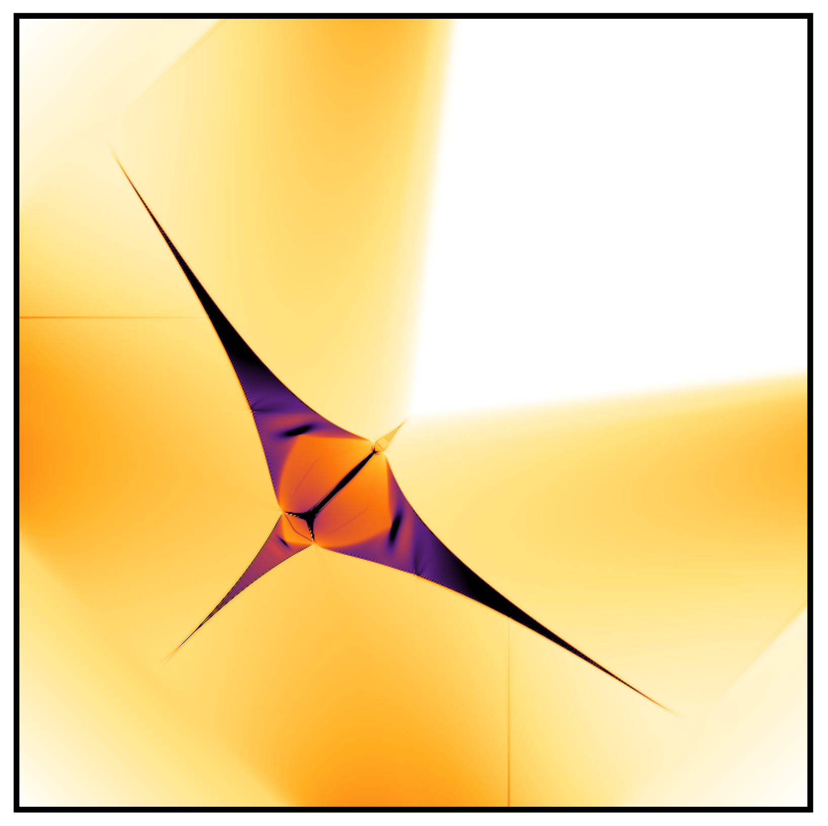
The numerical simulations are demonstrated in Section 5. While restricting to a quadratic domain $\Omega$, for four different loading conditions we perform a case study with respect to the Poisson ratio. Computational details, including mesh resolution, CPU time, and the obtained value functions, are listed in the tables.

The last section is devoted to the additional insight into the optimal membrane problem in the special case of the Michell energy potential $j=j^{\mathrm{M}}$. In this work, such framework is shown to be equivalent to working with the linearly isotropic material for $\nu=-1$. In Section 6.1 we explain how the Michell-energy setting can be additionally recast through the free material design formulation [18] provided that a particular set of admissible Hooke operators is chosen. Sections 6.2 and 6.3 revisit the results of [17] in order to recapitulate on the features of the pair ( P ) , ( P ∗ ) that are exclusive to this special choice of the energy potential. This includes the link to finding a metric that maximizes the Monge-Kanotrovich transport cost and an alternative numerical scheme by approximation through string systems. Finally, in Section 6.4 we show how a 2D optimal membrane design can can be exploited in solving a long standing problem in engineering optimization [67, 68, 57]: erecting an optimal 3D vault, a structure in pure compression that concentrates on a single surface. The present author has recently shown in [16] that such a construction can be rigorously made once $j=j^{\mathrm{M}}$ precisely.

The basic symbols used in the paper are listed in the index of notation. Below we explain in more details how vectors, matrices, and some of the differential operators are to be understood.

Elements $A\in\mathbb{R}^{m\times d}$ will be treated as matrices whose component in $i$-th row and $j$-th column is $A_{ij}$. Elements $\theta\in\mathbb{R}^{m}$ will be understood either as column vectors $[\theta_{1}\ \ldots\ \theta_{m}]^{\top}$ or as sequences of numbers $(\theta_{1},\ldots,\theta_{m})$, depending on the context. The tensor product $\theta\otimes\eta$ of two vectors $\theta,\eta\in\mathbb{R}^{m}$ is the quadratic matrix $A\in\mathbb{R}^{m\times m}$ of the components $A_{ij}=\theta_{i}\eta_{j}$. In Section 4 we will adapt a different notation for the vectors and matrices whose components $i$ and $j$ refer to $i$-th finite element and $j$-th node, respectively. Such vectors will be denoted in bold, e.g. ${\mathbf{q}}\in\mathbb{R}^{n}$, ${\mathbf{w}}\in\mathbb{R}^{m}$, ${\mathbf{D}}\in\mathbb{R}^{n\times m}$, and the components themselves will be written as ${\mathbf{q}}(i)$, ${\mathbf{w}}(j)$, ${\mathbf{D}}(i,j)$, etc.

For a smooth scalar function $w=w(x)=w(x_{1},\ldots,x_{d}):\mathbb{R}^{d}\to\mathbb{R}$ by the gradient $\nabla w$ we will mean the vector function $\theta:\mathbb{R}^{d}\to\mathbb{R}^{d}$ whose components are, point-wisely, $\theta_{i}=\frac{\partial w}{\partial x_{i}}$. For $m>1$ and a vector-valued function $u:\mathbb{R}^{d}\to\mathbb{R}^{m}$, the matrix-valued function $\xi=\nabla u:\mathbb{R}^{d}\to\mathbb{R}^{m\times d}$ is defined quite differently, namely $\xi_{ij}=\frac{\partial u_{i}}{\partial x_{j}}$. Note that we must not choose $m=1$ in the latter definition as it would give the transpose of the gradient defined for a scalar function. For a function $u:\mathbb{R}^{d}\to\mathbb{R}^{d}$ by $e(u)$ we understand the symmetric part of $\nabla u$, namely $\frac{1}{2}\big(\nabla u+(\nabla u)^{\top}\big)$.

For a bounded domain $\Omega\subset\mathbb{R}^{d}$ take Radon measures $\vartheta\in{\mathcal{M}}({\overline{\Omega}};\mathbb{R}^{d})$, ${\varsigma}\in{\mathcal{M}}({\overline{\Omega}};\mathbb{R}^{m\times d})$, $f\in{\mathcal{M}}({\overline{\Omega}};\mathbb{R})$, and $\mathcal{F}\in{\mathcal{M}}({\overline{\Omega}};\mathbb{R}^{m})$. We agree on the following definitions of the distributional divergences of vector- and, respectively, matrix-valued measures:

If $m=d$ and ${\varsigma}\in{\mathcal{M}}({\overline{\Omega}};\mathcal{S}^{d\times d})$, i.e. ${\varsigma}$ is valued in symmetric matrices, then above $\nabla\phi$ can be replaced by $e(\phi)$. If one assumes that $\vartheta,{\varsigma},f,\mathcal{F}$ are absolutely continuous with smooth densities $q,\sigma,\tilde{f},\tilde{\mathcal{F}}$, then (1.9) and (1.10) are equivalent to the equations $-\sum_{i}\frac{\partial q_{i}}{\partial x_{i}}=\tilde{f}$ and, respectively, $-\sum_{j}\frac{\partial\sigma_{ij}}{\partial x_{j}}=\tilde{\mathcal{F}}_{i}$, both holding in $\Omega$ only. Note that, due to the implied compactness of the supports of $\varphi,\phi$, no boundary conditions on ${\partial\Omega}$ follow from (1.9) or (1.10).

In most of the text the above notation will be adopted for $d=m=2$. In particular, $\Omega$ will be a domain in $\mathbb{R}^{2}$. In several places we will take a detour to three dimensional elasticity, and then we will use the under-bar symbol $\underaccent{\bar}{\argu}$ to distinguish 3D objects from the 2D ones, for example ${\underaccent{\bar}{\Omega}}\subset\mathbb{R}^{3},\underaccent{\bar}{\sigma}:{\underaccent{\bar}{\Omega}}\mapsto\mathcal{S}^{3\times 3}$, etc.

Let us agree that $\xi\in{\mathcal{S}^{2\times 2}}$ and $\sigma\in{\mathcal{S}^{2\times 2}}$ will stand for, respectively, the in-plane strain and the in-plane stress in the membrane. We depart from an elastic energy potential $j:{\mathcal{S}^{2\times 2}}\to\mathbb{R}_{+}$ that will be assumed to satisfy the conditions:

1. (H1)

   $j$ is real valued, non-negative and convex;

2. (H2)

   $j$ is positively $p$-homogeneous for a fixed exponent $p\in(1,\infty)$;

3. (H3)

   there exist positive constants $C_{1},C_{2}$ such that

   $$C_{1}{\left\lvert\xi\right\rvert}^{p}\leq j(\xi)\leq C_{2}{\left\lvert\xi\right\rvert}^{p}\qquad\forall\,\xi\in{\mathcal{S}^{2\times 2}}.$$

It is worth noting that existence of $C_{2}$ is already guaranteed by assumptions (H1) and (H2). It is also well established that $j$ must be continuous, see [65]. By $j^{*}:{\mathcal{S}^{2\times 2}}\to\overline{\mathbb{R}}=[-\infty,\infty]$ we will denote the convex conjugate of $j$, cf. Appendix A. By virtue of [65, Corollary 15.3.1] the function $j^{*}$ is convex positively $p^{\prime}$-homogeneous where $p^{\prime}=\frac{p}{p-1}$. On top of that, $j^{*}$ is also continuous and satisfies the bounds $\widetilde{C}_{2}{\left\lvert{\sigma}\right\rvert}^{p^{\prime}}\leq j^{*}({\sigma})\leq\widetilde{C}_{1}{\left\lvert{\sigma}\right\rvert}^{p^{\prime}}$ for suitably chosen $\widetilde{C}_{1},\widetilde{C}_{2}>0$.

An elastic material that is modelled by the energy potential $j$ is capable of withstanding both tension and compression, i.e. for any stress $\sigma\in{\mathcal{S}^{2\times 2}}$ the constitutive relation $\sigma\in\partial j(\xi)$ holds true for at least one strain $\xi\in{\mathcal{S}^{2\times 2}}$. In what follows, from a similar perspective we will analyse the relaxed energy potential

(note that, thanks to the lower bound in (H3), we have coerciveness of $j$, and thus attainment of the minimum follows). Earlier in Section 1.2, the energy $j_{+}$ was introduced as a relaxation of $j$, crucial from the point of view of the well-posedness of the Föppl’s membrane problem. In the process, the matrix $\zeta$ was interpreted as a strain correction aimed at lowering the stored energy and realized by means of fine-scale wrinkling. Apart from the mathematical properties of the relaxed potential, the following result is to show that $j_{+}$ is a modification of the initial energy potential $j$ which guarantees that the stress is purely tensile. Namely, the constitutive law ${{\sigma}}\in\partial j_{+}(\xi)$ implies that $\sigma\in{\mathcal{S}^{2\times 2}_{+}}$. Indeed, we will show that – on the dual side – the modification $j_{+}$ is aimed at penalizing non-tensile stresses $\sigma\notin{\mathcal{S}^{2\times 2}_{+}}$ exactly.

References

• Alberti and Ambrosio [1999] Alberti G, Ambrosio L (1999) A geometrical approach to monotone functions in ℝd\mathbb{R}^{d}. Math Z 230:259–316
• Allaire [2002] Allaire G (2002) Shape optimization by the homogenization method. Springer Science & Business Media
• Allaire and Kohn [1993] Allaire G, Kohn RV (1993) Optimal design for minimum weight and compliance in plane stress using extremal microstructures. Eur J Mech A-Solids 12:839–878
• Allaire et al [2004] Allaire G, Jouve F, Toader AM (2004) Structural optimization using sensitivity analysis and a level-set method. J Comput Phys 194:363–393
• Ambrosio et al [2000] Ambrosio L, Fusco N, Pallara D (2000) Functions of bounded variation and free discontinuity problems. Clarendon Press, Oxford
• Andersen et al [2003] Andersen ED, Roos C, Terlaky T (2003) On implementing a primal-dual interior-point method for conic quadratic optimization. Math Program 95:249–277
• ApS [2021] MOSEK ApS (2021) MOSEK optimization toolbox for MATLAB. User’s guide and reference manual, Release 9.2.35
• Babadjian et al [2023] Babadjian JF, Iurlano F, Rindler F (2023) Shape optimization of light structures and the vanishing mass conjecture. Duke Math J 172:43–103
• Barrett and Prigozhin [2007] Barrett JW, Prigozhin L (2007) A mixed formulation of the Monge-Kantorovich equations. Esaim Math Model Numer Anal 41:1041–1060
• Belgacem et al [2002] Belgacem HB, Conti S, DeSimone A, Müller S (2002) Energy scaling of compressed elastic films – three-dimensional elasticity and reduced theories. Arch Ration Mech Anal 164:1–37
• Bella and Kohn [2014] Bella P, Kohn RV (2014) Wrinkles as the result of compressive stresses in an annular thin film. Comm Pure Appl Math 67:693–747
• Ben-Tal and Nemirovski [2001] Ben-Tal A, Nemirovski A (2001) Lectures on modern convex optimization: analysis, algorithms, and engineering applications. SIAM
• Bendsøe et al [1994] Bendsøe MP, Guedes JM, Haber RB, Pedersen P, Taylor JE (1994) An analytical model to predict optimal material properties in the context of optimal structural design. J Appl Mech 61:930–937
• Bergos [1999] Bergos J (1999) Gaudí: The man and his work. Bulfinch Press
• Bołbotowski [2021] Bołbotowski K (2021) Elastic bodies and structures of the optimum form, material distribution, and anisotropy. Ph.D. thesis, Warsaw University of Technology
• Bołbotowski [2022] Bołbotowski K (2022) Optimal vault problem – form finding through 2D convex program. Comput Math Appl 109:280–324
• Bołbotowski and Bouchitté [2022] Bołbotowski K, Bouchitté G (2022) Optimal design versus maximal Monge–Kantorovich metrics. Arch Ration Mech Anal 243:1449–1524
• Bołbotowski and Lewiński [2022] Bołbotowski K, Lewiński T (2022) Setting the free material design problem through the methods of optimal mass distribution. Calc Var Partial Differ Equ 61:76
• Bouchitté [2020] Bouchitté G (2020) Optimization of light structures: the vanishing mass conjecture. arXiv preprint arXiv:200102022
• Bouchitté and Buttazzo [2001] Bouchitté G, Buttazzo G (2001) Characterization of optimal shapes and masses through Monge-Kantorovich equation. J Eur Math Soc 3:139–168
• Bouchitté and Fragalà [2003] Bouchitté G, Fragalà I (2003) Second-order energies on thin structures: variational theory and non-local effects. J Funct Anal 204:228–267
• Bouchitté and Fragalà [2007a] Bouchitté G, Fragalà I (2007a) Optimal design of thin plates by a dimension reduction for linear constrained problems. SIAM J Control Optim 46:1664–1682
• Bouchitté and Fragalà [2007b] Bouchitté G, Fragalà I (2007b) Optimality conditions for mass design problems and applications to thin plates. Arch Ration Mech Anal 184:257–284
• Bouchitté et al [1997] Bouchitté G, Buttazzo G, Seppecher P (1997) Energies with respect to a measure and applications to low dimensional structures. Calc Var Partial Differ Equ 5:37–54
• Bouchitté et al [2003] Bouchitté G, Buttazzo G, De Pascale L (2003) A p-Laplacian approximation for some mass optimization problems. J Optim Theory Appl 118:1–25
• Bouchitté et al [2008] Bouchitté G, Gangbo W, Seppecher P (2008) Michell trusses and lines of principal action. Math Models Meth Appl Sci 18:1571–1603
• Bouchitté et al [2014] Bouchitté G, Fragalà I, Lucardesi I (2014) Shape derivatives for minima of integral functionals. Math Program 148:111–142
• Caddock and Evans [1989] Caddock B, Evans K (1989) Microporous materials with negative Poisson’s ratios. I. Microstructure and mechanical properties. J Phys D: Appl Phys 22:1877–1882.
• Ciarlet [1980] Ciarlet PG (1980) A justification of the von Kármán equations. Arch Ration Mech Anal 73:349–389
• Ciarlet [2000a] Ciarlet PG (2000a) Mathematical Elasticity: Volume I: Three-Dimensional Elasticity. North-Holland
• Ciarlet [2000b] Ciarlet PG (2000b) Mathematical Elasticity: Volume II: Theory of Plates. North-Holland
• Ciarlet [2002] Ciarlet PG (2002) The finite element method for elliptic problems. SIAM
• Conti et al [2006] Conti S, Maggi F, Müller S (2006) Rigorous derivation of föppl’s theory for clamped elastic membranes leads to relaxation. SIAM J Math Anal 38:657–680
• Courant and Hilbert [1924] Courant R, Hilbert D (1953) Methods of mathematical physics. Interscience Publishers, New York
• Czarnecki [2015] Czarnecki S (2015) Isotropic material design. Computational Methods in Science and Technology 21:49–64
• Czarnecki and Lewiński [2012] Czarnecki S, Lewiński T (2012) A stress-based formulation of the free material design problem with the trace constraint and single loading condition. Bulletin of the Polish Academy of Sciences: Technical Sciences 60:191–204
• Czarnecki and Lewiński [2013] Czarnecki S, Lewiński T (2013) On minimum compliance problems of thin elastic plates of varying thickness. Struct Multidiscip Optim 48:17–31
• Czarnecki and Lewiński [2017] Czarnecki S, Lewiński T (2017) On material design by the optimal choice of Young’s modulus distribution. Int J Solids Struct 110:315–331
• Czubacki and Lewiński [2015] Czubacki R, Lewiński T (2015) Topology optimization of spatial continuum structures made of nonhomogeneous material of cubic symmetry. J Mech Mater Struct 10:519–535
• Czubacki and Lewiński [2020] Czubacki R, Lewiński T (2020) Optimal archgrids: a variational setting. Struct Multidiscip Optim 62:1371–1393
• Dzierzanowski and Czubacki [2021] Dzierzanowski G, Czubacki R (2021) Optimal archgrids spanning rectangular domains. Comput Struct 242:106371
• Ekeland and Temam [1999] Ekeland I, Temam R (1999) Convex analysis and variational problems. SIAM, Oxford
• Evans and Gariepy [1992] Evans L, Gariepy R (1992) Measure theory and fine properties of functions. CRC Press, Boca Raton
• Föppl [1907] Föppl A (1907) Vorlesungen über technische Mechanik. Vol. 5, Princeton University Press
• Fox et al [1993] Fox DD, Raoult A, Simo JC (1993) A justification of nonlinear properly invariant plate theories. Arch Ration Mech Anal 124:157–199
• Friesecke et al [2006] Friesecke G, James RD, Müller S (2006) A hierarchy of plate models derived from nonlinear elasticity by Gamma-convergence. Arch Ration Mech Anal 180:183–236
• Giaquinta and Giusti [1985] Giaquinta M, Giusti E (1985) Researches on the equilibrium of masonry structures. Arch Ration Mech Anal 88(4):359–392
• Goffman and Serrin [1964] Goffman C, Serrin J (1964) Sublinear functions of measures and variational integrals. Duke Math J 31:159–178
• Golay and Seppecher [2001] Golay F, Seppecher P (2001) Locking materials and the topology of optimal shapes. Eur. J. Mech. A-Solids 20:631–644
• Haslinger et al [2010] Haslinger J, Kočvara M, Leugering G, Stingl M (2010) Multidisciplinary free material optimization. SIAM J Appl Math 70:2709–2728
• Jiang et al [2018] Jiang Y, Zegard T, Baker WF, Paulino GH (2018) Form-finding of grid-shells using the ground structure and potential energy methods: a comparative study and assessment. Struct Multidiscip Optim 57:1187–1211
• von Kármán [1910] von Kármán T (1910) Festigkeitsprobleme im Maschinenbau in Encyclopädie der mathematischen Wissenschaften. vol. IV/4. Leipzig, pp 311–385
• Kohn and Strang [1986] Kohn RV, Strang G (1986) Optimal design and relaxation of variational problems, I, II, III. Comm Pure Appl Math 39:113–137, 139–182, 353–377
• Kohn and Vogelius [1984] Kohn RV, Vogelius M (1984) A new model for thin plates with rapidly varying thickness. Int J Solids Struct 20:333–350
• Kohn and Vogelius [1986] Kohn RV, Vogelius M (1986) Thin plates with rapidly varying thickness, and their relation to structural optimization. In: Homogenization and effective moduli of materials and media, Springer, pp 126–149
• Le Dret and Raoult [1995] Le Dret H, Raoult A (1995) The nonlinear membrane model as variational limit of nonlinear three-dimensional elasticity. J Math Pures Appl 74:549–578
• Lewiński et al [2019] Lewiński T, Sokół T, Graczykowski C (2019) Michell Structures. Springer International Publishing, Cham
• Lewiński et al [2023] Lewiński T, Rybka P, Zatorska-Goldstein A (2023) The free material design problem for the stationary heat equation on low dimensional structure. Nonlinearity 36:4501
• Merigot and Thibert [2021] Merigot Q, Thibert B (2021) Optimal transport: discretization and algorithms. In: Handbook of Numerical Analysis, vol. 22, Elsevier, pp 133–212
• Petersson [1999] Petersson J (1999) A finite element analysis of optimal variable thickness sheets. SIAM J Numer Anal 36:1759–1778
• Plotnikov and Sokolowski [2023] Plotnikov PI, Sokolowski J (2023) Geometric aspects of shape optimization. Geom Funct Anal 33:206
• Prall and Lakes [1997] Prall D, Lakes R (1997) Properties of a chiral honeycomb with a Poisson’s ratio of −1-1. Int J Mech Sci 39:305–314
• Ringertz [1993] Ringertz UT (1993) On finding the optimal distribution of material properties. Struct Optim 5:265–267
• Rockafellar [1968] Rockafellar R (1968) Integrals which are convex functionals. Pac J Math 24:525–539
• Rockafellar [1970] Rockafellar R (1970) Convex analysis. 28, Princeton University Press
• Rockafellar [1971] Rockafellar R (1971) Integrals which are convex functionals. II. Pac J Math 39:439–469
• Rozvany and Prager [1979] Rozvany GIN, Prager W (1979) A new class of structural optimization problems: optimal archgrids. Comput Meth Appl Mech Eng 19:127–150
• Rozvany et al [1982] Rozvany GIN, Wang CM, Dow M (1982) Prager-structures: archgrids and cable networks of optimal layout. Comput Meth Appl Mech Eng 31:91–113
• Santambrogio [2015] Santambrogio F (2015) Optimal transport for applied mathematicians. Birkäuser, New York
• Sokołowski and Zolésio [1992] Sokołowski J, Zolésio JP (1992) Introduction to shape optimization. Springer
• Temam [1985] Temam R (1985) Mathematical problems in plasticity. Paris
• Tobasco [2021] Tobasco I (2021) Curvature-driven wrinkling of thin elastic shells. Arch Ration Mech Anal 239:1211–1325
• Villani [2003] Villani C (2003) Topics in optimal transportation. American Mathematical Soc.
• Zalinescu [2002] Zalinescu C (2002) Convex analysis in general vector spaces. World Scientific