Copula for Instance-wise Feature Selection and Ranking
Abstract
Instance-wise feature selection and ranking methods can achieve a good selection of task-friendly features for each sample in the context of neural networks. However, existing approaches that assume feature subsets to be independent are imperfect when considering the dependency between features. To address this limitation, we propose to incorporate the Gaussian copula, a powerful mathematical technique for capturing correlations between variables, into the current feature selection framework with no additional changes needed. Experimental results on both synthetic and real datasets, in terms of performance comparison and interpretability, demonstrate that our method is capable of capturing meaningful correlations.
1 Introduction
The primary goal of feature selection is to select the most relevant features, and simultaneously help benefit the downstream tasks like recognition [Nilsson et al. 2007, Stańczyk and Jain 2015], clustering [Dash and Liu 2000, Liu and Yu 2005, Witten and Tibshirani 2010]. Traditional approaches view feature selection and downstream tasks as two separate entities. However, recent methods based on neural networks have achieved greater performance by combining the two, resulting in a differentiable optimization. Furthermore, the importance of features can vary from sample to sample; one set of features may be useful for recognizing one thing, while a completely different set of features may be necessary to identify something else. Therefore, it is necessary for feature selection to be done on a case-by-case basis, which is known as instance-wise feature selection [Yoon et al. 2019, Chen et al. 2018, Masoomi et al. 2020], it selects unique features for each sample.
Characteristics in reality are often correlated, such as a person’s height and weight, economic status and wealth, etc. The identification of feature correlations can minimize the redundancy of features. Yet, in the literature of instance-wise feature selection and ranking methods [Chen et al. 2018, Yoon et al. 2019, Abid et al. 2019, Masoomi et al. 2020, Wu and Liu 2018] that follow the context of neural networks, the dependencies between features has not been considered manifestly. For instance, L2X [Chen et al. 2018] performs a feature selection for maximizing the mutual information between selected feature subsets and corresponding outputs. Lowering the KL distance between the selected features and all features, is the guideline of INVASE [Yoon et al. 2019]. However, little or even no consideration in modeling correlations can pose a challenge to tasks.
To address this matter, we underscore the importance of capturing the pairwise relationship between features, and explicitly model it through a probabilistic framework. This paper examines both binary feature selection and top- feature ranking. Specifically, for the top- feature ranking problem, the number of features chosen is assumed to be known and unchanging. However, for binary feature selection, the number of features varies across samples, as different samples may have different feature significance. For both scenarios, two sampling policies are presented in the paper, along with a corresponding neural network implementation to unite feature selection and task learning.
Our contributions are summarized as follows:
- •
We explore the explicit dependence between features through copula, such as instance-wise feature selection and top- ranking, as the initial step.
- •
Two sampling schemes, implemented via neural networks, have been carefully crafted to ensure accuracy and efficiency. Moreover, they have been rigorously tested and verified to guarantee their efficacy.
- •
The experimental results have been found to be highly indicative and of superior quality, as evidenced by metrics such as accuracy, true positive rate (TPR), and false discovery rate (FDR). Indeed, these results demonstrate a remarkable explanatory power.
2 Preliminaries and Related Work
Notation: Lowercase typeface letters () represent scalar, lowercase bold typeface letters () represent vectors, uppercase typeface letters () stand for random variable, uppercase bold typeface letters () represent matrix.
2.1 Feature Selection
In recent decades, feature selection has evolved from a specialized field to a commonplace technology in the machine learning community [Guyon and Elisseeff 2003, Koller and Sahami 1996, Liu and Motoda 2007], and has been employed to simplify systems and make them more interpretable to researchers [Guyon and Aliferis 2007, Brown et al. 2012]. Existing works on instance-wise feature selection can be divided into two main categories: binary feature selection [Chen et al. 2018, Yoon et al. 2019] and top- feature ranking [Abid et al. 2019, Yamada et al. 2020]. The distinction between them is that the number of binary feature selection is dependent on the instance, while the number of top- feature ranking is user-defined and known. Our work is akin to Yoon et al. 2019 and [Chen et al. 2018], in that all have a 3-stage network structure. Sokar et al. 2022 is based on sparse autoencoders and uses a new sparse training algorithm to quickly attend to informative features, but does not provide theoretical analysis or justification for the algorithm. The second method, called Stochastic Gates Yamada et al. 2020, selects a small subset of features based on probabilistic relaxation of the ‘0 norm, and simultaneously learns a non-linear regression or classification function. However, it does not provide a direct differentiable top-k feature selection method and does not explore the correlation between features in a differentiable manner. Nevertheless, none of the aforementioned works have explicitly modeled the dependency; instead, we propose incorporating a Gaussian copula into binary feature selection and top- feature ranking.
2.2 Reminders on Copula
Copula [Cherubini et al. 2004, Trivedi and Zimmer 2007, Jaworski et al. 2010] is a powerful tool for describing the correlation between variables by modelling their joint distributions, given the known marginal distributions where each variable follows the uniform distribution . It can be combined with a variational auto-encoder (VAE) to address the issue of posterior collapse in the latent space [Wang and Wang 2019]. On the other side, Wang and Yin 2020 introduces a new distribution called the relaxed multivariate Bernoulli distribution (RelaxedMVB), which is a reparameterizable relaxation of the multivariate Bernoulli distribution. The RelaxedMVB combines the Gaussian copula and the Relaxed Bernoulli to create a continuous relaxation of the multivariate Bernoulli distribution. Furthermore, Suh and Choi 2016 proposed to employ Gaussian copula to model the local dependency. Additionally, copula has been extensively applied in finance applications [Cherubini et al. 2004, Cherubini et al. 2011].
We briefly review the copula theory. For any continuous random variables, , let their marginal distributions be correspondingly. Then it is easy to see that follows the uniform distribution on for . And the copula of is defined as the joint cumulative distribution function (C.D.F) of .
is a function from to . We can rewrite the above formula as:
One of the most helpful copula is known as the Gaussian copula, which is constructed from a multivariate normal distribution over by using the probability integral transform. Its explicit formula is given as
where is the joint cdf of multivariate normal distribution with mean zero and correlation/covariance matrix , is the inverse of a set of marginal Gaussian cdf. Off-diagonal elements in capture pairwise relation between different marginals.
3 Method
In this section, we shall commence by presenting the problem statement. Thereafter, we shall introduce two sampling schemes for binary feature selection and top- feature ranking, respectively. Subsequently, we shall provide the overall algorithm workflow. Lastly, we shall discuss the details of implementing neural networks in greater detail.
3.1 Problem Formulation
Given a collection of samples , where is a -dimension feature vector, is the corresponding output. Feature selection seeks to select a subset of features and simultaneously learn a task-specific objective function under certain loss metrics as follows:
| subject to |
where denote the learnable parameters, represents the learned score, represents the element-wise product, stands for the feature indicator, is the objective function, represents the sampling function, and stand for the mapping function to learn and infer prediction, respectively. For top- feature ranking, since the specific size of active features is established, we add an auxiliary constraint to loss function. In contrast, the number of binary feature selection is sample-dependent, the regularization term that controls selected features number, where is the trade-off parameter.
The above expression shows that the selection of features is dictated by the variable . Also on the other hand, is depended on . Thus the final performance is greatly affected by the way how we model . Due to expressive power and complexity of neural network, we naturally introduce neural network e.g. multilayer perceptron (MLP) to learn the mapping .
Despite we have known how to parameterize , sampling function usually is non-differentiable, as non-differentiable methods may have a large variance. It will hinder the usage of standard back-propagation algorithm and has large variance. Besides, mostly assumes elements of to be independent, like Gumbel-Softmax [Jang et al. 2017]. To address the first issue, we develop two sampling schemes as a continuous differentiable approximation to Bernoulli distribution and top- ranking without replacement. To address the second issue, we incorporate the copula function to model the dependency between features explicitly. In what follows, we drop the superscript for simplicity.
3.2 Sampling Scheme via Binary Mask
When the number of features is unknown and sample-dependent, for each , we define a binary-valued random variable which indicates whether the -th feature should be included in . Specifically, follows this distribution: and . Here ’s are obtained from weight layer.
By Gumbel-Max trick, we know that and have the same distribution, where and follow a standard logistic distribution. ’s follow the uniform distribution , and each element is independent to the other during the generation procedure in the classical Gumbel-Max algorithm. Also, as we can see, is an indicator function and hence is not differentiable with respect to . To circumvent this issue, we consider to replace by its soft counterpart, that is, . Here is a tuning parameter. When , it is not hard to see that .
In addition to characterizing the marginal distribution, we need to take into account the dependence among different ’s. It suffices to model the joint distribution of ’s. To do so, we incorporate a copula to accommodate its dependence structure. We write the joint C.D.F. of as . We assume the following parameterized form, , where is a Gaussian copula with as its correlation matrix and . In a summary, () is the output of the feature selection layer.
A natural question is how to guarantee the correlation matrix to be positive definite. We consider the following parameterization scheme. From the perspective of factor analysis [Harman 1976, Kline 2014], suppose a random vector lies in a lower-dimensional manifold:
where is a latent random -vector and is the coefficient/loading matrix with size being . Suppose and are mutually uncorrelated, covariance matrix of is an identity and the noise level of is , then we know
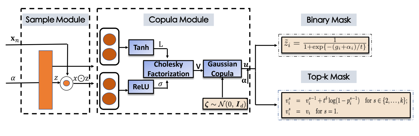
In other words, we can parameterize the correlation matrix as , where function maps a covariance matrix to a correlation matrix and satisfies . By adopting this parametrization, it’s guaranteed that the correlation matrix is positive definite. Procedure to obtain correlated noise via Gaussian copula is summarized in Algorithm 1, algorithm flow for binary feature selection in Algorithm 2. The proposed sampling scheme is first proposed in Wang and Yin 2020 and our sampling scheme is identical to this.
3.3 Sampling Scheme via Top- Ranking
When the number of features is known, without loss of generality, we let (). We aim to find the top- features with the most predictive power. Suppose we have obtained the weights from weight layer. A straightforward way to select the features randomly proportional to its weights, which is also known as the weighted random sampling (WRS) [Xie and Ermon 2019]. This procedure can be realized through the following ways: (i) For each , sample independently and compute keys . (ii) Select features with the largest keys .
Firstly, we can observe that are sampled independently in above procedure. We extend this by adding correlations between ’s. That is, their joint distribution satisfies
| (1) |
where correlation matrix should be learned through the network. Here, we assume admits the structure with as a hyper parameter controlling the magnitude of correlations. Observe to ourselves that certain equivalence of here and in (3.2) by giving .
Secondly, suppose the top- active feature set based on keys is . We then define the indicator to represent whether feature is selected or not. By such construction, we know that is not a differentiable function of ’s. This may bring difficulty in computing the backward gradients. To avoid this problem, we consider a continuous deterministic relaxation to approximate ’s. The specific procedure is described as follows. We define
for , where is defined recursively by
Here is a tuning parameter that determines the approximation level and is a hyper-parameter that adjusts the step size. We then define the relaxed value of which is and let . By writing into the vector form, we have
with . Via using this relaxation scheme, our method contains the classical weighted random sampling as special case. The algorithm workflow for top- ranking method is listed in Algorithm 3. On top of the above, we offer the following two theorems to shed light on role of in the convergence of the sampling scheme, with the proofs deferred to the Appendix.
Theorem 3.1.
As both , we have .
Here, “" represents the convergence in distribution. Function chooses the indices of largest elements in provided the length of is at least . When , the proposed converges to which follows the weighted sampling distribution. On the other hand, if we take and let , then the proposed method can also recover the situation top sampling based on weights .
Proof of Theorem 3.1.
Let be and it suffices to show that
| (2) | |||||
By recursive formula of , it can directly verified that for any , there exists a constant such that
| (3) |
holds when . Here, is defined to be the set of indices of largest keys . (Here is called as the key for -th feature.) In other words, returns the indices of top keys when .
On the other hand, when , we know that the correlation matrix converges to . By Fubini’s Theorem and following the proof strategy of Proposition 3 in Efraimidis and Spirakis 2006, we know that
| (4) |
Theorem 3.2.
When , we have as both , where .
Proof of Theorem 3.2.
Similar to the proof of Theorem 3.1, we again know that returns the indices of top keys when . It remains to show that the order of ’s is the same as the order of ’s when .
We only need to show that the probability that, for any pair , it holds
| (5) |
if . By straightforward calculation, we get
The right hand side goes to 0 as . This leads to the desired result. ∎
3.4 The Overall Architecture
We now turn to the detailed implementation via neural networks, which merges the deep neural networks and the proposed framework of feature selection.
As illustrated in Figure 1, our architecture is composed of three parts: (i) ChoiceNet (abbreviation of Choice Network), which models the mapping and is responsible for selecting features and outputting the learned score for each sample. (ii) Sampler Module, which models the sampling function and receives the input to output , where indicates that the -th feature is preserved or otherwise removed, and the selected feature can be expressed as . (iii) PredictNet (abbreviation of Predictor Network), which receives the selected feature as input and outputs the corresponding prediction. For further details on the practical applications of this architecture in terms of neural networks, please refer to the Appendix.
3.4.1 Architecture of ChoiceNet and PredictNet
Both ChoiceNet and CriticNet are three-layer MLPs with ReLU [Brownlee 2019] or SeLU [Klambauer et al. 2017] activations. For ChoiceNet, the size of the input layer is , a fully connected layer with the dimension of is added after the input layer, and the dimension of the final layer is also equivalent to . PredictNet differs from ChoiceNet in that the number of units in the last layer is , where is the number of labels for classification tasks, and is the dimension of the hidden layer. Additionally, a Softmax layer is added to the last layer for prediction, and Batch Normalization is added after the activation function to reduce overfitting.
3.4.2 Architecture of Sampler Module
Architecture of Binary Sampler Module
It is not straightforward to implement a copula using a neural network, as the covariance matrix must be guaranteed to be positive semi-definite (PSD). To this end, two extra fully connected layers are included to infer and , with tanh and relu activation functions applied after the fully connected layer. After obtaining the covariance function, Cholesky decomposition can be used to obtain the factor matrix , ensuring that the covariance matrix is PSD. During the inference stage, a Bernoulli distribution is sampled for each sample. Algorithm 2 can be leveraged to generate the feature indicator vector, as illustrated in Figure 2.
Architecture of Top- Sampler Module
WRS generates the key for the associated feature as . By taking the log transformation, the key can be written as , since the log transformation is monotonic, the induced construction of is still consistent with the original key . For concrete realization, we propose to reparameterize the key as a deterministic mapping of the parameters and via a neural network. Then, by leveraging the top- relaxation in Algorithm 3, we can build a differentiable approximation with respect to the key . The architecture of the top- sampling scheme in the context of neural networks is similar to that of binary feature selection, except for the block representation. We also provide a demonstration of the block in Figure 2.
4 Experimental Results
In this section, we empirically compare our algorithm with the advanced feature selection methods. For binary feature selection, we quantitatively compare our work with several powerful algorithms including methods based on neural networks like INVASE [Yoon et al. 2019], L2X [Chen et al. 2018], LIME [Ribeiro et al. 2016], Shap [Lundberg and Lee 2017], Knockoff [Barber and Candès 2015], and classical methods like Tree [Geurts et al. 2006], SCFS [Hall 2000], LASSO [Tibshirani 1996]. For top- feature selection, we also validate our algorithm with several dominant approaches such as STG [Yamada et al. 2020], CAE [Abid et al. 2019], L2X [Chen et al. 2018], Shap [Lundberg and Lee 2017], LASSO [Tibshirani 1996], RF [Díaz-Uriarte and De Andres 2006], boosting [Friedman et al. 2000]. In the comparison of classical methods, the advantages of neural network-based methods in an end-to-end fashion are highlighted. It should be noted that, although these approaches vary in type, they all serve the purpose of feature selection, which is also widely employed in the preceding methods. See Appendix for the details of implementation and baseline methods.
| Dataset | Syn1 | Syn2 | Syn3 | Syn4 | Syn5 | Syn6 | ||||||
|---|---|---|---|---|---|---|---|---|---|---|---|---|
| Metric | TPR | FDR | TPR | FDR | TPR | FDR | TPR | FDR | TPR | FDR | TPR | FDR |
| Ours | 100.0 | 0.0 | 86.4 | 4.8 | 96.8 | 2.0 | 95.5 | 2.0 | 89.3 | 3.78 | 93.8 | 6.6 |
| INVASE [Yoon et al. 2019] | 100.0 | 0.0 | 100.0 | 0.0 | 92.0 | 0.0 | 99.8 | 10.3 | 84.8 | 1.1 | 90.1 | 7.4 |
| L2X [Chen et al. 2018] | 100.0 | 0.0 | 100.0 | 0.0 | 69.4 | 30.6 | 79.5 | 21.8 | 74.8 | 26.3 | 83.3 | 16.7 |
| Shap [Lundberg and Lee 2017] | 60.4 | 39.6 | 93.3 | 6.7 | 90.9 | 9.1 | 65.2 | 31.9 | 62.9 | 33.7 | 71.2 | 28.8 |
| LIME [Ribeiro et al. 2016] | 13.8 | 86.2 | 100.0 | 0.0 | 98.1 | 1.9 | 40.7 | 49.4 | 41.1 | 50.6 | 50.5 | 49.5 |
| Knockoff [Barber and Candès 2015] | 10.0 | 70.0 | 8.7 | 36.2 | 81.2 | 17.5 | 38.8 | 35.1 | 41.0 | 51.1 | 56.6 | 42.1 |
| Tree [Geurts et al. 2006] | 100.0 | 0.0 | 100.0 | 0.0 | 100.0 | 0.0 | 54.7 | 39.0 | 56.8 | 37.5 | 60.0 | 40.0 |
| LASSO [Tibshirani 1996] | 19.0 | 81.0 | 39.8 | 60.2 | 78.3 | 21.7 | 49.9 | 50.9 | 45.5 | 48.2 | 56.4 | 43.6 |
| SCFS [Hall 2000] | 23.5 | 76.5 | 39.5 | 60.5 | 78.3 | 22.0 | 48.9 | 52.4 | 42.4 | 51.2 | 56.1 | 43.9 |
| Dataset | Syn1 | Syn2 | Syn3 | Syn4 | Syn5 | Syn6 | ||||||
|---|---|---|---|---|---|---|---|---|---|---|---|---|
| Metric | TPR | FDR | TPR | FDR | TPR | FDR | TPR | FDR | TPR | FDR | TPR | FDR |
| Ours | 100.0 | 0.0 | 100.0 | 0.0 | 100.0 | 1.2 | 94.5 | 40.3 | 88.4 | 9.4 | 99.5 | 14.6 |
| INVASE [Yoon et al. 2019] | 100.0 | 0.0 | 100.0 | 0.0 | 100.0 | 0.0 | 66.3 | 40.5 | 73.2 | 23.7 | 90.5 | 15.4 |
| L2X [Chen et al. 2018] | 6.1 | 93.9 | 81.4 | 18.6 | 57.7 | 42.3 | 48.5 | 46.5 | 35.4 | 60.8 | 66.3 | 33.7 |
| Shap [Lundberg and Lee 2017] | 4.4 | 85.6 | 95.1 | 4.9 | 88.8 | 11.2 | 50.2 | 43.4 | 49.9 | 44.2 | 62.5 | 37.5 |
| LIME [Ribeiro et al. 2016] | 0.0 | 100.0 | 100.0 | 0.0 | 92.7 | 7.3 | 43.8 | 47.4 | 49.9 | 44.2 | 50.1 | 49.9 |
| Knockoff [Barber and Candès 2015] | 0.0 | 64.9 | 3.7 | 71.2 | 74.9 | 24.9 | 28.2 | 59.8 | 33.1 | 59.4 | 46.9 | 53.0 |
| Tree [Geurts et al. 2006] | 49.9 | 50.1 | 100.0 | 0.0 | 100.0 | 0.0 | 40.7 | 49.5 | 56.7 | 37.5 | 58.4 | 41.6 |
| LASSO [Tibshirani 1996] | 2.5 | 97.5 | 4.0 | 96.0 | 75.3 | 24.7 | 28.3 | 73.2 | 36.0 | 56.9 | 45.9 | 54.1 |
| SCFS [Hall 2000] | 2.5 | 97.5 | 5.3 | 94.7 | 74.9 | 25.1 | 27.0 | 74.6 | 30.6 | 62.1 | 38.3 | 61.7 |
| Dataset | Syn1 | Syn2 | Syn3 | Syn4 | Syn5 | Syn6 | ||||||
|---|---|---|---|---|---|---|---|---|---|---|---|---|
| Metric | TPR | FDR | TPR | FDR | TPR | FDR | TPR | FDR | TPR | FDR | TPR | FDR |
| Ours | 100.0 | 0.0 | 100.0 | 0.0 | 100.0 | 0.0 | 91.95 | 41.6 | 90.9 | 42.0 | 90.1 | 43.9 |
| NOLA | 74.8 | 18.3 | 96.4 | 16.7 | 99.7 | 78.4 | 48.5 | 84.0 | 66.8 | 49.3 | 50.0 | 46.2 |
| INVASE [Yoon et al. 2019] | 69.3 | 27.5 | 93.6 | 14.5 | 91.8 | 72.5 | 62.5 | 87.3 | 46.2 | 53.8 | 37.9 | 41.7 |
We begin our experiments with six challenging synthetic datasets as suggested in INVASE [Yoon et al. 2019]. ’s are sampled from a multivariate Gaussian distribution with 11 dimensions, and the covariance matrix is an identity matrix. is dependent on informative and relevant features in , and is set as a Bernoulli random variable that is 1 with probability . By varying , we can generate different values across datasets.
- •
Syn1:
- •
Syn2:
- •
Syn3:
- •
Syn4: if , , otherwise, .
- •
Syn5: if , , otherwise, .
- •
Syn6:if , , otherwise, .
We generate 10,000 samples for training and 10,000 samples for testing. The response in the Syn1, Syn2, and Syn3 datasets is determined by the identical subset of features. In contrast, the number of relevant features differs across samples in the Syn4, Syn5, and Syn6 datasets; performance on these datasets can demonstrate the ability of methods to detect instance-wise and population-aware features. We evaluate the performance in terms of true positive rate (TPR) and false discovery rate (FDR). As shown in Table 1, our method achieves comparable or even better performance than the previous best method INVASE [Yoon et al. 2019] on Syn1 and Syn3 datasets, demonstrating its capability in selecting relevant features for real data. Moreover, on Syn5 and Syn6 datasets, which are specifically designed for instance-wise feature selection, our algorithm outperforms INVASE [Yoon et al. 2019] in terms of instance-wise feature selection.
4.0.1 100-dimensional Synthetic Dataset
To further demonstrate the generality of our framework, we experimented on the 100-dimensional synthetic dataset, adding 89 auxiliary, unrelated features and increasing the feature dimension to 100, while still keeping the produced features uncorrelated. As illustrated in Table 2, our method remains the best-performing approach across most datasets.
4.0.2 Correlated Feature Selection
We use the same dataset in Section 4.0.1, but with a specially designed covariance matrix , where and denote the indices of features. To validate whether copula can capture the dependence between features, we compare our method with INVASE, the best competing baseline approach, and a variant of our method, NOLA (No cOpuLA), where only copula is removed from our framework. The results in Table 3 demonstrate that copula performs better than both INVASE and NOLA.
4.1 Feature Ranking Experiments on Real Datasets
4.1.1 Dataset Description
MNIST is a hand-digital dataset comprising 50,000 training samples and 10,000 test samples, drawn from ten classes. Fashion-MNIST is a clothing dataset, containing 60,000 training samples and 10,000 test samples. ISOLET is a speech dataset for predicting which letter-name was spoken, and it includes approximately 8,000 samples with 617 features. We randomly split it into the training set and test set in a 75-25 ratio. The dimensions and sample sizes of the data are summarized in Table 4.
| Dataset | dimension | size | type | labels |
|---|---|---|---|---|
| MNIST | 784 | 60k | Image | 10 |
| Fashion MNIST | 784 | 70k | Image | 10 |
| ISOLET | 617 | 7.8k | Audio | 26 |
We now turn to instance-wise top- feature ranking on real datasets, including MNIST [LeCun 1998], Fashion MNIST [Xiao et al. 2017], and the ISOLET dataset [Cole et al. 1990]. For details of the datasets, ablation studies, and visualization results, please refer to the Appendices.
We measure performance by utilizing accuracy metrics and compare each method varying the number of selected features. Figure 3 shows the resulting prediction accuracy, which mostly outperforms other baselines, indicating that our method is a strong candidate in selecting top- predictive features. The impact of copula and low-rank approximation on final performance is also investigated in the Appendix.

4.2 Instance-wise Binary Feature Selection on Synthetic Datasets
4.3 Visualization on PSD Matrix
To provide an intuitive illustration of the structure of the PSD matrix, we conducted an experiment on the MNIST dataset using copula to perform instance-wise feature selection. We then utilized t-SNE [van der Maaten and Hinton 2008] on the induced PSD matrix to visualize the structure. The left image in Figure 4 provides a demonstration; we can observe that the features with label 0 and label 1 are well separable, since these labels are not similar. Additionally, features with labels 4, 7, and 9 are close to each other, due to their similar appearance. The visualization reflects that the PSD matrix indeed captures the intrinsic character of the feature.
As illustrated in the geometry structure of on the MNIST dataset for binary feature selection, we provide another visualization on the PSD matrix for top- feature ranking. Following the same profile in Section 4.1, we set to 40 while keeping all other experimental parameters unchanged. The middle image of Figure 4 shows a similar experimental phenomenon and leads to the same conclusion, indicating that the learned can effectively capture the correlated relationship.
We also visualize on the Fashion-MNIST dataset, as shown in the right image of Figure 4. We observe that the low-dimensional embeddings of Sneaker and Ankle boot are close, as they share similar characteristics. The same conclusion applies to Coat and Pullover, while the embeddings for Trouser are more concentrated and distant from the other image embeddings. This illustrates that copula can effectively capture the relationship between features. Further visualizations can be found in the Appendix.
4.4 Ablation Studies
4.4.1 Effects of Low-Rank Approximation
We conducted experiments on the MNIST dataset with varying sizes of low-rank approximations. When we performed top- feature ranking, we set equal to . The results are presented in Table 5, which demonstrate that low-rank approximations can achieve comparable performance to a full-rank scheme. Despite the time-consuming nature of low-rank approximations, whose time complexity is , the value of the Gaussian copula cannot be overlooked.
| Dataset | MNIST | ||
|---|---|---|---|
| k | 10 | 20 | 30 |
| Full-rank | 91.77 | 92.94 | 93.57 |
| Low-rank | 91.34 | 92.40 | 93.93 |
4.4.2 Effects of Copula in Top- Feature Ranking
To investigate the effect of copula on the ultimate performance of top- feature ranking, we conducted an experiment in accordance with the same protocol outlined in Section 4.0.2, wherein only the copula was removed from the framework while all other experimental settings remained the same (hereafter referred to as NOLA). We tested our method on the MNIST dataset, and the results are summarized in Table 6. It is evident that our approach significantly enhances the performance when compared to NOLA.
| Dataset | MNIST | |||
|---|---|---|---|---|
| k | 10 | 20 | 30 | 40 |
| Ours | 91.77 | 92.94 | 93.57 | 93.79 |
| NOLA | 86.93 | 87.61 | 88.90 | 92.73 |
5 Conclusion
In this paper, we have explored the potential of capturing the relationship between correlated features for binary feature selection and top- feature ranking. To this end, we have successfully incorporated Gaussian copula into the existing feature selection framework with minimal modifications. Our proposed implementation via neural networks has yielded promising results, outperforming many classical and leading methods. We are confident that our work will inspire further research into more effective methods for mining the correlation between features. Possible future directions include capturing tail dependency in features with more sophisticated copulas, or the correlations can be generated via an implicit generative model [Janke et al. 2021].
Appendix A Analysis with respect to complexity
The computational complexity can be estimated as , where is the number of features. Since we have to do matrix decomposition. To reduce the computational complexity even further, additional techniques can be applied. As one of the proposed solutions in the article Lee et al. 2022, we can threshold the correlation matrix , and grouping features based on agglomerative clustering using the correlation matrix as the similarity measure. This reduces the number of computations required by conducting block-wise matrix multiplication, which scales quadratically with respect to the largest block size (i.e., the number of features grouped in the largest block). By maintaining the correlation structure within each group, the generated gates for features within the same group can be used to select features that are highly correlated with the target variable, while reducing the computational complexity of the algorithm. If the largest block size remains the same, the complexity of generating the correlated gate vectors will only increase linearly with the feature dimension (since the number of blocks would increase linearly).
The CPU calculation time for copula-based feature selection also depends on the implementation, hardware, and software used. To reduce CPU calculation time, some techniques such as parallelization and approximation methods can be used. For example, using GPU computation can significantly speed up feature selection process, particularly for large datasets.
In summary, copula-based feature selection can be computationally expensive, particularly for large datasets with many features. The computational complexity can be estimated as , and the CPU calculation time depends on the implementation, hardware, and software used. However, optimization techniques such as parallelization and approximation methods can be used to reduce the computational complexity and CPU calculation time.
Appendix B Visualization of Chosen Pixels
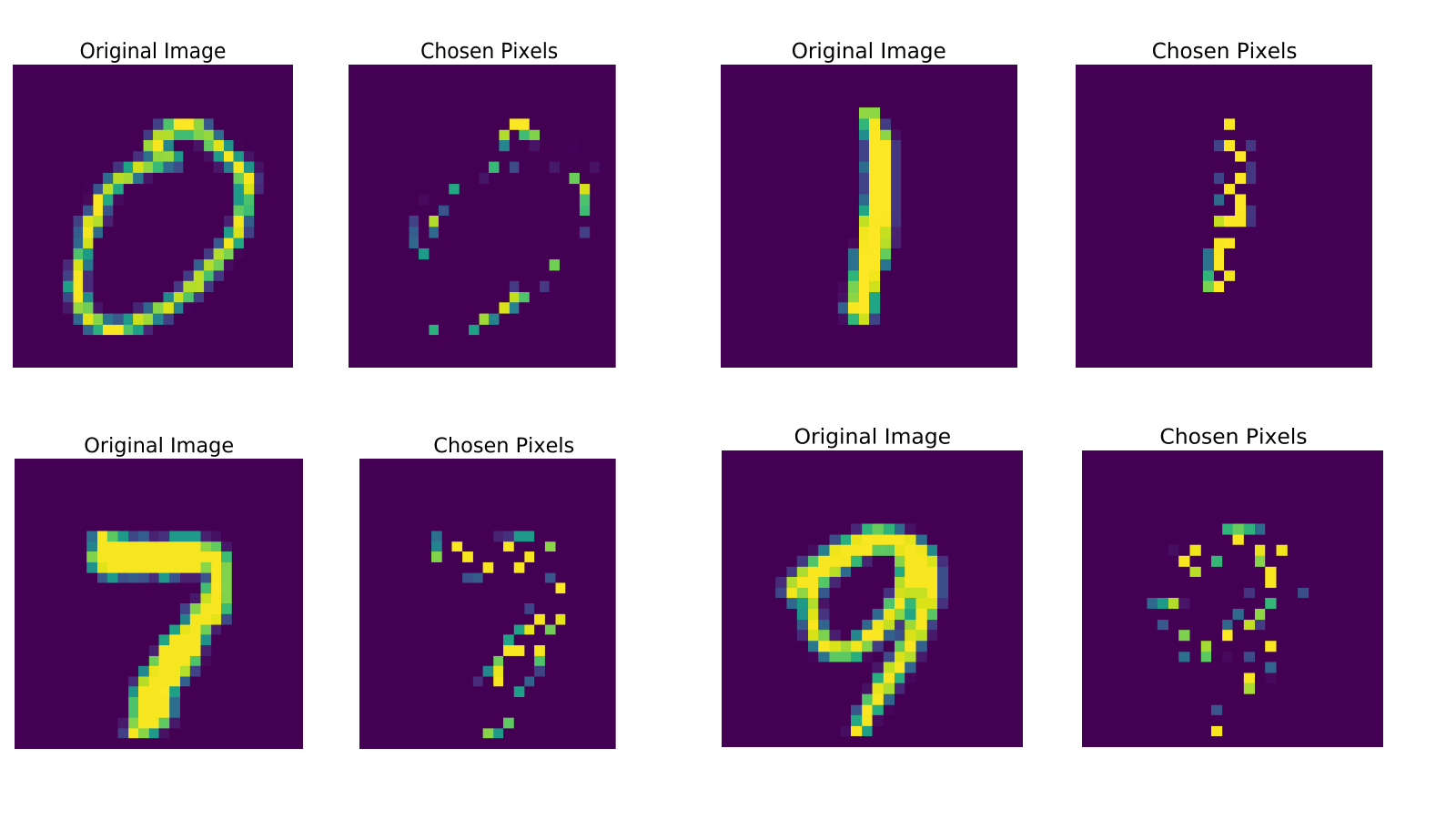
Now, we present a visual representation of the top-120 features with the most significant values in the for each sample on the MNIST dataset. For each image, we display the most informative features. As is evident from Figure 5, we can observe a clear segmentation in the shape of the classification object, indicating that our method is capable of identifying the most important and meaningful features. This visualization demonstrates the remarkable interpretive power of our method.
Appendix C Neural Reparameterization of Correlated Uniform Noise
In Algorithm 4, we present the workflow to produce correlated uniform noise . Here, we offer a further elucidation of the neural reparameterization of it. We denote the output of the hidden layer in ChoiceNet as as , and the weight parameter of the layer which produces as . Additionally, stands for the weight parameter of the layer which generates matrix . If we opt for the low-rank approximation, the shape of is , otherwise . The concrete implementation via neural reparameterization is provided as follows:
Appendix D Details of Baseline Methods
The summary of some baseline methods of binary feature selection are as follows.
- •
Xgboost We used the Gini index as the splitting criterion. Specifically, we used the DecisionTreeClassifier function from the scikit-learn library with default parameters. The DecisionTreeClassifier function builds a decision tree by recursively splitting the data based on the feature with the highest Gini importance score. The Gini importance score measures the total reduction of impurity brought by a feature in the decision tree, and features with higher Gini importance scores are considered more important. After building the decision tree, we selected the top- features with the highest Gini importance scores as the selected features. The value of was determined using the same experimental setup and evaluation protocol as our proposed method.
LASSO In the paper, LASSO is a linear regression-based feature selection method, where we used regularization to encourage sparsity in the model coefficients. Specifically, we used the LogisticRegression function from the scikit-learn library with penalty and default parameters. The penalty in the LogisticRegression function encourages sparsity in the model coefficients by adding a penalty term to the loss function that is proportional to the absolute value of the coefficients. This penalty term forces the model to select only a subset of the most important features, effectively performing feature selection. After fitting the logistic regression model with regularization, we selected the top- features with the highest absolute coefficients as the selected features. The value of was determined using the same experimental setup and evaluation protocol as our proposed method, including a hold-out strategy and 5-fold cross-validation for hyperparameter tuning.
- •
L2X [Chen et al. 2018] introduces a new model interpretation way from the feature selection perspective, it aims to learn a feature selection network that maximizes the mutual information between selected feature subsets and corresponding outputs, we use the official implementation to evaluate the result from the link:
https://github.com/Jianbo-Lab/L2X
- •
INVASE [Yoon et al. 2019] proposes an instance-wise feature selection algorithm based on the actor-critic framework to selects most relevant features that minimizes the Kullback-Leibler (KL) divergence between full conditional distribution and suppressed feature distribution, we use the official implementation to evaluate the result from the link:
https://github.com/jsyoon0823/INVASE
- •
LIME [Ribeiro et al. 2016] is a model-agnostic explanation algorithm, it learns an interpretable model locally in a non-redundant and faithful manner by formulating the task as a submodular optimization problem, we use the official implementation to evaluate the result from the link:
https://github.com/marcotcr/lime
- •
Shap [Lundberg and Lee 2017] proposes a novel framework that employs the shapely value to calculate the feature importance, we use the official implementation to evaluate the result from the link:
https://github.com/slundberg/shap
- •
Knockoff [Barber and Candès 2015] aims to find which variables are important to the response by comparison between knock-off variables and original variables. we use the official implementation to evaluate the result from the link:
http://web.stanford.edu/group/candes/knockoffs/software/knockoff/
In our experiments, we used a neural network as the predictive model in conjunction with Shap and LIME. The neural network had the same size and architecture as the one in our proposed method, in order to ensure fairness and exclude the influence of other factors such as network architecture and size. Regarding the cutoffs, we used a threshold of 0.5 for the neural network to predict the binary class labels. We applied the same threshold when generating the Shap and LIME explanations, to ensure consistency in the interpretation of feature importance across different methods.
The description of some baseline methods of top- feature ranking are as follows:
- •
STG [Yamada et al. 2020] provides a novel algorithm that depends on the Gaussian-based relaxation of the Bernoulli distribution to select relevant features, we use the official implementation to evaluate the result from the link:
https://github.com/runopti/stg
- •
CAE [Abid et al. 2019] introduces an auto-encoder architecture for global feature selection while reconstructing the input, we use the official implementation to evaluate the result from the link:
https://github.com/mfbalin/Concrete-Autoencoders
D.1 Discussions of Baseline Methods
Our method is capable of discerning pertinent features on a global scale (Syn1, Syn2, and Syn3) as well as on an individual basis (Syn4, Syn5, and Syn6). Notably, our approach surpasses prior neural network-based approaches (INVASE, L2X) in terms of individual performance, with the improvement being more pronounced in Syn4 and Syn5 than in Syn6. Random Forests (RFs) can select global features, thus performing better on Syn1, Syn2, and Syn3, but not as well on Syn4, Syn5, and Syn6. Shapley-based methods calculate the variable importance to elucidate the linear dependency for each sample; however, it is difficult to capture the non-linear relationships in synthetic data, thus rendering it less effective in high-dimensional data. LIME utilizes simple functions to interpret complexity locally; however, it can only explain the particular instance, meaning that it may not be able to accommodate for unseen instances. Knockoff filters features according to certain criteria, yet there is no assurance that this metric is uniquely optimal, thus its performance may vary across datasets.
Appendix E Implementation Details
E.1 Synthetic Datasets
We have employed the same datasets and network structure as in Yoon et al. 2019. For all experiments on the six synthetic datasets, the hyperparameters and were set to 100 and 200, respectively. The activation function of the last layer was a sigmoid. The entire network (ChoiceNet and PredictNet) was trained for 1,000 epochs using Adam with a batch size of 1,000, a weight decay of 0.001, and coefficients of 0.9 and 0.999 for computing running averages of gradient and its square. The constant learning rate was set to 0.0001, and the temperature parameter was set to either 3 or 5. Finally, cross-validation was employed to tune the hyperparameter .
E.2 Real Datasets
When performing top- feature ranking, and were both set to 16. In all the experiments, we discovered that the Cholesky decomposition to obtain the Cholesky factor matrix was time-consuming, so we employed the full-rank scheme. We trained the network for 100 epochs using Adam, with coefficients used for computing running averages of gradient set to 0.9 and 0.999. The constant learning rate was set to 0.001 for Fashion-MNIST and MNIST, and 0.0001 for ISOLET. The batch size was set to 1,000 for MNIST and Fashion-MNIST, and 64 for ISOLET, while the temperature was set to for all the experiments evaluated on real datasets. All the parameters of the neural networks were randomly initialized. For a fair comparison with baseline methods based on neural networks such as INVASE, L2X, STG, and CAE, we employed the same hyper-parameters and architecture to evaluate the performance.
References
- Abid et al. [2019] Abubakar Abid, Muhammad Fatih Balin, and James Zou. Concrete autoencoders for differentiable feature selection and reconstruction. arXiv preprint arXiv:1901.09346, 2019.
- Barber and Candès [2015] Rina Foygel Barber and Emmanuel J Candès. Controlling the false discovery rate via knockoffs. The Annals of Statistics, 43(5):2055–2085, 2015.
- Brown et al. [2012] Gavin Brown, Adam Craig Pocock, Ming-Jie Zhao, and Mikel Luján. Conditional likelihood maximisation: A unifying framework for information theoretic feature selection. J. Mach. Learn. Res., 13:27–66, 2012.
- Brownlee [2019] Jason Brownlee. A gentle introduction to the rectified linear unit (relu). Machine learning mastery, 6, 2019.
- Chen et al. [2018] Jianbo Chen, Le Song, Martin J. Wainwright, and Michael I. Jordan. Learning to explain: An information-theoretic perspective on model interpretation. In Proceedings of the 35th International Conference on Machine Learning (ICML), pages 882–891, Stockholmsmässan, Stockholm, Sweden, 2018.
- Cherubini et al. [2004] Umberto Cherubini, Elisa Luciano, and Walter Vecchiato. Copula Methods in Finance. John Wiley & Sons, 2004.
- Cherubini et al. [2011] Umberto Cherubini, Sabrina Mulinacci, Fabio Gobbi, and Silvia Romagnoli. Dynamic Copula Methods in Finance. John Wiley & Sons, 2011.
- Cole et al. [1990] Ron Cole, Yeshwant Muthusamy, and Mark Fanty. The ISOLET spoken letter database, 1990.
- Dash and Liu [2000] Manoranjan Dash and Huan Liu. Feature selection for clustering. In Proceedings of the 4th Pacific-Asia Conference on Knowledge Discovery and Data Mining, Current Issues and New Applications (PADKK), pages 110–121, Kyoto, Japan, 2000.
- Díaz-Uriarte and De Andres [2006] Ramón Díaz-Uriarte and Sara Alvarez De Andres. Gene selection and classification of microarray data using random forest. BMC bioinformatics, 7(1):1–13, 2006.
- Efraimidis and Spirakis [2006] Pavlos S Efraimidis and Paul G Spirakis. Weighted random sampling with a reservoir. Information Processing Letters, 97(5):181–185, 2006.
- Friedman et al. [2000] Jerome H. Friedman, Trevor J. Hastie, and Robert Tibshirani. Additive logistic regression: a statistical view of boosting. The Annals of Statistics, 28(2):337–407, 2000.
- Geurts et al. [2006] Pierre Geurts, Damien Ernst, and Louis Wehenkel. Extremely randomized trees. Mach. Learn., 63(1):3–42, 2006.
- Guyon and Aliferis [2007] Isabelle Guyon and Constantin Aliferis. Causal feature selection. In Computational Methods of Feature Selection, pages 79–102. Chapman and Hall/CRC, 2007.
- Guyon and Elisseeff [2003] Isabelle Guyon and André Elisseeff. An introduction to variable and feature selection. J. Mach. Learn. Res., 3(Mar):1157–1182, 2003.
- Hall [2000] Mark A. Hall. Correlation-based feature selection for discrete and numeric class machine learning. In Proceedings of the Seventeenth International Conference on Machine Learning (ICML), pages 359–366, Stanford, CA, 2000.
- Harman [1976] Harry H Harman. Modern Factor Analysis. University of Chicago press, 1976.
- Jang et al. [2017] Eric Jang, Shixiang Gu, and Ben Poole. Categorical reparameterization with gumbel-softmax. In Proceedings of the 5th International Conference on Learning Representations (ICLR), Toulon, France, 2017.
- Janke et al. [2021] Tim Janke, Mohamed Ghanmi, and Florian Steinke. Implicit generative copulas. In Advances in Neural Information Processing Systems (NeurIPS), pages 26028–26039, Virtual, 2021.
- Jaworski et al. [2010] Piotr Jaworski, Fabrizio Durante, Wolfgang Karl Hardle, and Tomasz Rychlik. Copula Theory and its Applications, volume 198. Springer, 2010.
- Klambauer et al. [2017] Günter Klambauer, Thomas Unterthiner, Andreas Mayr, and Sepp Hochreiter. Self-normalizing neural networks. In Advances in Neural Information Processing Systems (NIPS), pages 971–980, Long Beach, CA, 2017.
- Kline [2014] Paul Kline. An Easy Guide to Factor Analysis. Routledge, 2014.
- Koller and Sahami [1996] Daphne Koller and Mehran Sahami. Toward optimal feature selection. In Proceedings of the Thirteenth International Conference on Machine Learning (ICML), pages 284–292, Bari, Italy, 1996.
- LeCun [1998] Yann LeCun. The mnist database of handwritten digits. http://yann. lecun. com/exdb/mnist/, 1998.
- Lee et al. [2022] Changhee Lee, Fergus Imrie, and Mihaela van der Schaar. Self-supervision enhanced feature selection with correlated gates. In International Conference on Learning Representations, 2022.
- Liu and Motoda [2007] Huan Liu and Hiroshi Motoda. Computational Methods of Feature Selection. CRC Press, 2007.
- Liu and Yu [2005] Huan Liu and Lei Yu. Toward integrating feature selection algorithms for classification and clustering. IEEE Trans. Knowl. Data Eng., 17(4):491–502, 2005.
- Lundberg and Lee [2017] Scott M. Lundberg and Su-In Lee. A unified approach to interpreting model predictions. In Advances in Neural Information Processing Systems (NIPS), pages 4765–4774, Long Beach, CA, 2017.
- Masoomi et al. [2020] Aria Masoomi, Chieh Wu, Tingting Zhao, Zifeng Wang, Peter J. Castaldi, and Jennifer G. Dy. Instance-wise feature grouping. In Advances in Neural Information Processing Systems (NeurIPS), virtual, 2020.
- Nilsson et al. [2007] Roland Nilsson, José M. Peña, Johan Björkegren, and Jesper Tegnér. Consistent feature selection for pattern recognition in polynomial time. J. Mach. Learn. Res., 8:589–612, 2007.
- Ribeiro et al. [2016] Marco Tulio Ribeiro, Sameer Singh, and Carlos Guestrin. “why should I trust you?”: Explaining the predictions of any classifier. In Proceedings of the 22nd ACM SIGKDD International Conference on Knowledge Discovery and Data Mining (KDD), pages 1135–1144, San Francisco, CA, 2016.
- Sokar et al. [2022] Ghada Sokar, Zahra Atashgahi, Mykola Pechenizkiy, and Decebal Constantin Mocanu. Where to pay attention in sparse training for feature selection? arXiv preprint arXiv:2211.14627, 2022.
- Stańczyk and Jain [2015] Urszula Stańczyk and Lakhmi C Jain. Feature Selection for Data and Pattern Recognition. Springer, 2015.
- Suh and Choi [2016] Suwon Suh and Seungjin Choi. Gaussian copula variational autoencoders for mixed data. arXiv preprint arXiv:1604.04960, 2016.
- Tibshirani [1996] Robert Tibshirani. Regression shrinkage and selection via the lasso. Journal of the Royal Statistical Society: Series B (Methodological), 58(1):267–288, 1996.
- Trivedi and Zimmer [2007] Pravin K Trivedi and David M Zimmer. Copula Modeling: an Introduction for Practitioners. Now Publishers Inc, 2007.
- van der Maaten and Hinton [2008] Laurens van der Maaten and Geoffrey Hinton. Visualizing data using t-SNE. J. Mach. Learn. Res., 9(86):2579–2605, 2008.
- Wang and Wang [2019] Prince Zizhuang Wang and William Yang Wang. Neural gaussian copula for variational autoencoder. In Proceedings of the 2019 Conference on Empirical Methods in Natural Language Processing and the 9th International Joint Conference on Natural Language Processing (EMNLP-IJCNLP), pages 4332–4342, Hong Kong, China, 2019.
- Wang and Yin [2020] Xi Wang and Junming Yin. Relaxed multivariate bernoulli distribution and its applications to deep generative models. In Conference on Uncertainty in Artificial Intelligence, pages 500–509. PMLR, 2020.
- Witten and Tibshirani [2010] Daniela M Witten and Robert Tibshirani. A framework for feature selection in clustering. Journal of the American Statistical Association, 105(490):713–726, 2010.
- Wu and Liu [2018] Liang Wu and Huan Liu. Tracing fake-news footprints: Characterizing social media messages by how they propagate. In Proceedings of the Eleventh ACM International Conference on Web Search and Data Mining (WSDM), pages 637–645, Marina Del Rey, CA, 2018.
- Xiao et al. [2017] Han Xiao, Kashif Rasul, and Roland Vollgraf. Fashion-mnist: a novel image dataset for benchmarking machine learning algorithms. arXiv preprint arXiv:1708.07747, 2017.
- Xie and Ermon [2019] Sang Michael Xie and Stefano Ermon. Reparameterizable subset sampling via continuous relaxations. In Proceedings of the Twenty-Eighth International Joint Conference on Artificial Intelligence (IJCAI), pages 3919–3925, Macao, China, 2019.
- Yamada et al. [2020] Yutaro Yamada, Ofir Lindenbaum, Sahand Negahban, and Yuval Kluger. Feature selection using stochastic gates. In Proceedings of the 37th International Conference on Machine Learning (ICML), pages 10648–10659, Virtual Event, 2020.
- Yoon et al. [2019] Jinsung Yoon, James Jordon, and Mihaela van der Schaar. INVASE: instance-wise variable selection using neural networks. In Proceedings of the 7th International Conference on Learning Representations (ICLR), 2019.