Marvin Jahn
Address: Department of Mathematics
Technical University of Munich
Boltzmannstr. 3
85748 Garching b. München
Germany
Email: marvin.jahn@tum.de and Peter Massopust
Address: Department of Mathematics
Technical University of Munich
Boltzmannstr. 3
85748 Garching b. München
Germany
Email: massopust@ma.tum.de
Abstract.
We introduce the novel concept of integral Read-Bajraktarević (iRB) operator and discuss some of its properties. We show that this iRB operator generalizes the known Read-Bajraktarević (RB) operator and we derive conditions for the fixed point of the iRB operator to belong to certain function spaces.
Key words and phrases:
Fractal interpolation, Read-Bajraktarević operator, fixed point, function space
1991 Mathematics Subject Classification
Primary 47H10; Secondary 28A80, 41A30, 54A50
1. Introduction
The idea of interpolating a given set of data points by well-behaved functions is a prominent and very important concept in many areas of mathematics and the natural sciences. Typical choices for such functions are, for instance, polynomials or splines, but one may also wish to interpolate the points using less smooth or even non-differentiable functions. This is the case when the data come from an underlying model that describes highly irregular and complex signals or images.
This desire to approximate a data set by a non-smooth function leads to the concept of fractal interpolation originally introduced in [1] and in a slightly different setting in [7]. Since then, numerous variants of this concept have been studied. The interested reader is referred to the following albeit incomplete list of references regarding fractal interpolation and some of its applications: [2, 3, 4, 5, 6, 8, 9, 10, 11, 13, 14, 15]. More pointers to the flexibility and versatility of fractal interpolation theory are found in the literature part of these papers.
For some of these variations, the focus has shifted from trying to interpolate certain points to the general construction of fractal functions given some parameters. This is also the setup considered in [12], an approach which we seek to generalize in this paper.
In [12], a normed vector space , a Banach space and a subset are fixed and one is interested in finding a function satisfying functional equations of the form
(1.1)
where , , are certain fixed functions. Here and throughout the paper, we use the notation to denote the initial segment of length of the natural numbers .
One of the assumptions in [12] is that the functions are injective and that their images partition . (The case where some of the have points in common is treated in [14, 15].)
The functional equations (1.1) express a kind of self-referentiability that their solutions must exhibit. (Cf. for instance, [1, 10].) Thus, these solutions are also called fractal (interpolation) functions as the graph of is in general a fractal (set), i.e., a set with in general non-integral (box or Hausdorff) dimension.
A key realization is that finding a solution of (1.1) is equivalent to determining a fixed point of the Read-Bajraktarević (RB) operator [4, 14, 15] ,
(1.2)
where denotes a suitable subset of the vector space of all functions and the indicator or characteristic function of a set .
The key insight is to choose in such a way that it can be endowed with a metric (usually even a norm) such that becomes a complete metric space.
It suffices then to show that is a contraction on in order to establish the existence and uniqueness of a fixed point
of by the Banach fixed point theorem.
The novel idea presented in this paper is to replace the sums appearing in the RB operator (1) by integrals (with respect to Lebesgue measure). This leads us to the definition of an integral Read-Bajraktarević (iRB) operator,
a new concept that is formulated in Section2. In the subsequent Section 3, we introduce a method to extend a discrete collection of maps to a function which may be thought of as a family of functions for by a suitable homotopy.
This construction serves two purposes. On the one hand, we use it to specify in Section5 in what sense the iRB operator generalizes the RB operator (1), and on the other hand, it allows to present some concrete examples.
In Section4, we consider the case that , the subspace of consisting of bounded functions equipped with the supremum norm, and explore under what assumptions on the parameter functions , , and , we can guarantee that the iRB operator is a contraction on thus yielding a unique fixed point in by the Banach fixed point theorem.
In the subsequent Section5, we exhibit the RB operator (1) as a special case of the iRB operator. In the following section, we investigate under what conditions the bounded fixed point is continuous. Finally, in Section7, we turn our attention to the space of -functions, , endowed with the usual -norm and investigate under what assumptions the fixed point of the iRB operator exists and is unique.
2. An integral RB Operator
Throughout this paper, let denote a normed vector space, a Banach space, and a nonempty subset of . Moreover, let denote a fixed subset of the vector space of all functions , to be specified later.
Our first goal is to derive an “integral” version of the RB operator (1) described in the introduction.
To this end, we observe that the sums within the RB operator (1)
are just integrals with respect to counting measure .
Indeed, for a fixed , we may define in order to rewrite the first sum in (1) as
and similarly for the second sum. Thus, it seems natural to replace the sums by integrals with respect to Lebesgue measure:
We call this new mapping an integral Read-Bajraktarević (iRB) operator.
Note that just like the RB operator (1), the iRB operator consists of a linear part (the second term) and an affine part (the first term), i.e., it is also an affine operator.
Instead of functional equations (1.1), a fixed point of must now satisfy the integral equation
Therefore, we also call the fixed points of solutions.
Of course, the step of replacing sums by integrals requires modifying our setup.
Instead of injective functions for , we consider
a family of measurable functions such that the are injective for almost all .
Following the above notation, we write for the image of each of the again . However, we do not assume that the (for ) are disjoint or cover . Note that is zero whenever which means that those are not of particular interest.
In a similar way, we proceed with the and . Instead of such functions we now have two measurable functions and .
For , we call the sets
-hit times.
Thus, we may rewrite the iRB operator as follows:
(2.1)
Therefore, in order for the iRB operator to be well-defined, we have to require that is measurable for every . Otherwise, could be, e.g., the identity function on the Vitali set for every so that is the Vitali set for every and thus not measurable.
If is compact, then is closed and therefore measurable, as the following lemma shows.
Lemma 2.1.
Suppose that is compact and that is continuous.
Then the -hit times are closed for every .
Proof.
Let be a convergent sequence in , such that for every ,
there exists an with .
Since is compact, there exists a subsequence of
converging to some .
Replacing the original sequence with this subsequence,
we have , so that the continuity of yields ,
which had to be shown.
∎
It turns out that plays an important role in characterizing the behavior of the iRB operator. (See 4.1 below.)
Note that in the discrete setting, it is common to assume that the are pairwise disjoint for so that the discrete analogue of the -hit times is just a singleton for every .
3. Construction of an Extension
Having introduced the iRB operator, we now outline a method to construct a map given functions .
This new function is then an extension of the in the sense that
for all .
Our interest in this construction is motivated by the fact that it will allow us to understand the iRB operator
as a generalization of the RB operator (1).
Furthermore, it will enable us to easily provide some examples for the solutions that may arise for typical choices of
the parameter functions , and .
The construction relies on choosing a particular function ,
which we often just take to be the identity function .
Definition 3.1.
Let and be subsets of the normed vector spaces and , respectively, with being convex.
Furthermore, let be a function with and .
For a collection of functions (), define their extension with respect to to be the function
Here and below, denotes the floor function.
Intuitively, the function distributes the “influence” that and
have on . If is small, then “is close to” and
if is close to , then approximates .
The extension inherits some properties from the , which we summarize in the following lemma.
Lemma 3.2.
The extension given in 3.1 has the following properties:
(1)
If and all the are continuous, then is continuous.
(2)
If all are bounded by some positive constant, then is bounded by that same constant.
Proof.
(1)
Let be a sequence in the interval and a sequence in .
If then is constant for sufficiently large and the claim
follows by continuity of and all the .
In case that , we split the sequence into two subsequences with and , respectively. Then we show that both subsequences converge to the same limit by considering the following two cases:
Case 1: :
Then, for sufficiently large , we have
so since .
Case 2: :
Similarly, for sufficiently large , we observe that
showing that as .
(2)
This is immediate, because on each interval (), is a convex combination of
and . ∎
3.2 shows that if and all are continuous, then amounts to a
homotopy between and for every :
Note that the () resulting from our construction of the extension need not be injective, even if all () are injective. We now give a simple example demonstrating this phenomenon.
Example 3.3.
Let and a continuous function with and .
The affine linear functions
are injective and have the extension
By continuity of , the preimage is nonempty and any element in this preimage
has the property that is constant.
For instance, by choosing , we have .
Similarly, replacing by the injective function
yields the extension (for )
In this case, the quadratic polynomial is not injective if and only if its maximum lies in the interval ,
which turns out to be the case for .
This shows that it need not be the case that is injective for almost all ,
even though all are injective.
4. Bounded Solutions
We now seek bounded solutions for the iRB operator, that is, we ask under what conditions the iRB operator maps the Banach space
of bounded functions to itself and when it is a contraction.
Here, is equipped with the supremum norm .
Note that is certainly bounded if , and
are bounded.
Theorem 4.1.
Suppose that and are bounded.
Let be the supremum of and
denotes the maximal Lebesgue measure of all hit times .
If , then the iRB operator possesses a unique fixed point.
Proof.
As endowed with the supremum norm is a Banach space, it suffices to show that is a contraction, since the result is then a consequence of the Banach fixed point theorem.
By virtue of the constructive nature of the proof of the Banach fixed point theorem, we obtain immediately the following corollary.
Corollary 4.2.
The fixed point of the iRB operator from 4.1 is the limit of the iterates
, for , and an arbitrarily chosen .
Furthermore, we have the estimate
We illustrate the above theorem by hand of two examples.
Example 4.3.
Let and . Consider the affine linear functions
Their extension for is
(4.1)
For the inverse of is thus given by .
The -hit times trivially satisfy in 4.1.
Furthermore, we choose and set
Since , the theorem yields the existence of a unique fixed point of the iRB operator,
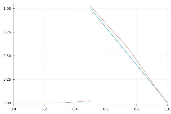
which is plotted in the figure below.
Figure 1. The graphs of the first (blue) and second (orange) iterate of the iRB operator,
when starting with the zero function. The third iterate (not plotted) is almost indistinguishable
from the second one . The estimate
from 4.2 for the fixed point implies that
“essentially looks like” (at least at this scale).
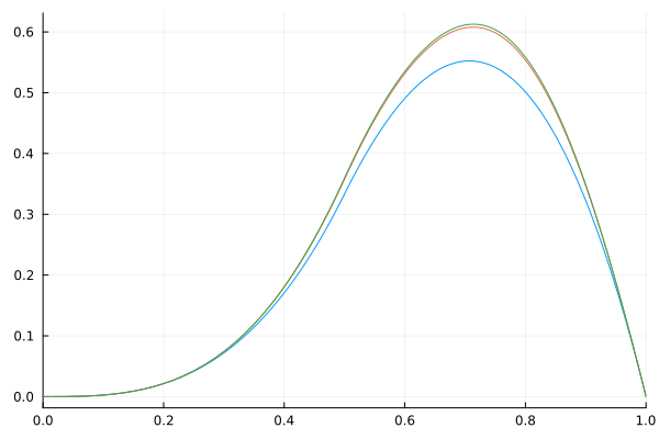
Figure 2. The graphs of the first (blue), second (orange) and third (green) iterate of the iRB operator,
when starting with the zero function.
These two examples show that depending on the choice of the parameter functions and ,
the solutions can have a smooth or discontinuous character.
In Section6, we derive a criterion guaranteeing continuity of the solution.
Furthermore, we will see in the next section that any solution of an RB operator can also be realized as a
solution of a corresponding iRB operator.
Therefore, the solutions of iRB operators can display the same “richness” in behavior as those of RB operators.
5. The iRB Operator as a Generalization of the RB Operator
The iRB operator can be seen to be a generalization of the RB operator (1) using the construction of an extension presented in 3.1.
To this end, let , and be given parameter functions of the RB operator (1),
which we want to exhibit as a special case of the iRB operator (2.1).
For , we denote the extensions of , and
by , , and , respectively.
This means that
and similarly for and .
In other words, for and , is equal to .
Furthermore, is equal to if and to for .
Notice that the situation is slightly asymmetrical because
agrees with the for on an interval of length (after projecting onto the first component),
whereas is equal to or only on an interval of length .
To remedy this, we need to replace by and do the same for , , and .
To simplify notation, we also set
for , , and .
Then, the iRB operator induced by , and agrees with the ordinary RB operator (1) for , , and :
We summarize our result in the next theorem.
Theorem 5.1(iRB operator generalizes the RB operator).
With , and constructed as above, their induced iRB operator is equal to
the RB operator of , and .
In particular, any function that is a solution of the RB operator can also be realized as a solution of the corresponding iRB operator.
A straightforward calculation shows that the parabola is a fixed point of .
We replace by , by ,
by and by
and then form the extensions , and with respect to .
By 5.1, the resulting iRB operator is precisely the RB operator .
As the iRB operator has a unique fixed point by 4.1,
the iterates (when, e.g., starting with the zero function)
must converge to this parabola.
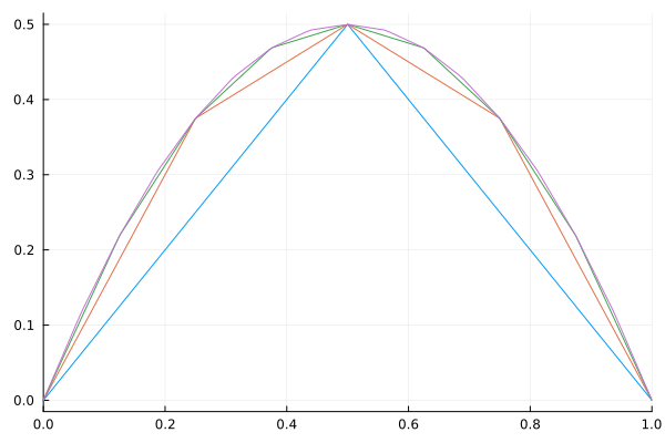
This is confirmed by plotting a couple of iterations.
Figure 3. The first four (blue, orange, green, purple) iterates of the iRB operator
when starting with the zero function. It is apparent that they converge to the parabola .
Similarly, we can realize the Takagi function (see [16]) as a fixed point of the iRB operator (by multiplying and in the previous example by ) as it is the fixed point of an RB operator.
It should be noted that the extensions , and in 5.1 are generally discontinuous
due to the discontinuity of at .
We might also want to understand the RB operator as a special case of the iRB operator
that is induced by continuous , and .
For this purpose, we set and assume that we are given continuous , and
inducing an RB operator as in (1).
Then the idea is to replace the expression for given above by a sequence of continuous functions
that converges pointwise to ;
for instance we can choose (for )
Applying the above construction (with respect to ) to , , and
(and again replacing by and similarly for , and )
yields a sequence of functions , , and .
However, two subtleties arise in this context.
On the one hand, we need to assume that is convex in order for to be a function
(instead of having codomain ), which is the setting we are interested in. (See Section2.)
On the other hand, we need to ensure that the extensions have the property that for every ,
is injective for almost all .
This is not automatically satisfied, as demonstrated by 3.3,
but it is guaranteed if the set
is a (Lebesgue) null set for all .
Hence, for every , we may construct a corresponding iRB operator .
By 3.2, all are induced by continuous , and .
This construction allows us to approximate the RB operator, as demonstrated by the following theorem.
Theorem 5.3(iRB operator approximates the RB operator).
Let be convex. For , let be injective and , be bounded.
Furthermore, assume that all these functions are continuous.
Denote their RB operator as defined in (1) by .
If for all , the set
is a null set, then the sequence of iRB operators constructed above
is well-defined.
It converges pointwise to the RB operator .
Proof.
We need to verify the pointwise convergence .
By 5.1, we can construct , and , such that the iRB operator induced
by them is equal to the RB operator .
Therefore, it suffices to show that .
Let , and set
and
so that . We employ a similar notation for to obtain and with . Then we have
By construction, agrees with for all .
The analogous statement is true for and .
Therefore, the first summand simplifies to
(5.1)
By 3.2, all and are bounded by .
Since this constant is independent of , and , (5.1) is bounded above by
The analogous argument applies to the second summand which establishes the assertion.
∎
In general, this convergence is not uniform, as the following example shows.
Additionally, we choose and .
Then the extension of the is and the extension of the is ,
so that the iRB operator is just
We construct , and as above and
note that and for all and .
Moreover, just like in the previous proof, we observe that
for and .
On the other hand, if
then , implying that
Note that contains for every , since
it is a closed interval of length with infimum between and .
Choosing such that , it follows that
where we used first and then made the substitution .
Therefore, for an arbitrary , we may choose which implies that
, showing that the convergence is not uniform.
6. Continuous Solutions
We now examine the continuity of the unique fixed point that is guaranteed by 4.1.
That is, we restrict the iRB operator to the space of bounded, continuous functions .
More precisely, we assume that and that all assumptions of 4.1 are satisfied and investigate what conditions guarantee that .
To that end, we consider a convergent sequence in
and first focus on the affine part
of the iRB operator.
As is bounded,
the dominated convergence theorem (for Bochner integrals) implies that
assuming the limit exists
for almost all .
Since we want to be continuous, we must ensure that this limit is equal to
.
For this purpose, we introduce the following terminology.
Given an arbitrary family of functions , their set of discontinuity times at is
If we demand that for every , the set of discontinuity times
is a null set and that the same is true for , then as desired
for almost all .
By the following lemma, the latter assumption can be simplified.
Lemma 6.1.
For , we have
Here, the boundary operator is understood with respect to .
Proof.
Assume that and consider the case that .
As (the closure of ) there exists a sequence that converges to such that is discontinuous at .
If instead , then there exists a sequence that converges to ;
for if not, then there must be some open neighborhood of in that is contained in ,
implying that is in the interior of .
On the other hand, suppose that .
If , then any sequence converging to must eventually lie in the complement of ,
so that is continuous at .
Similarly, if is in the interior of , then any sequence converging to must eventually lie in
that interior, showing that is continuous at .
∎
Therefore, for any , we have
and we demand that this latter set is a null set.
An analogous argument for the linear part
of the iRB operator shows that is continuous
if we additionally require and to be null sets for all .
Note that this is in particular the case when these functions are continuous for almost all .
Under these assumptions, the iRB operator restricts to and by applying the Banach fixed point theorem, we obtain a bounded continuous fixed point. By uniqueness, it must also be the fixed point of .
This establishes the following theorem.
Theorem 6.2.
Within the setting of 4.1,
assume further that for all , the discontinuity times , and are null sets
(which in particular is the case if these functions are continuous for almost all )
and that the set is also a null set for all .
Then, the unique fixed point of the iRB operator is continuous.
Example 6.3.
Returning to 4.3, we first observe that since
for , the set
contains at most two points and is thus a null set for all .
Let be a sequence converging to from below (so for all ). Then
implying , even though ,
which shows that is discontinuous at for all .
Therefore, the assumptions of 6.2 are not fulfilled.
Instead, the affine part of the iRB operator satisfies
and thus does not converge to
If is continuous, then the linear part of the iRB operator is continuous, as and are continuous for all .
Consequently, is discontinuous and in particular the unique fixed point must be discontinuous as well.
This is confirmed by Fig.1.
Example 6.4.
In 4.4, it is clear that , and are continuous, which together with the observation regarding
from the previous example implies that the solution must be continuous.
This is also apparent from Fig.2.
7. Solutions in
Let us now consider and with the usual Euclidean norm and the space (for ), which is equipped with the -norm
As before, we first need to ensure that maps from to ,
meaning that whenever .
To this end, we calculate (for arbitrary )
where we first utilized Jensen’s inequality and then the monotonicity of .
Another application of Jensen’s inequality reveals that
The second summand can be estimated analogously. Putting these inequalities together, we obtain
By Tonelli’s theorem, this is equal to
Assuming that is a diffeomorphism for almost all ,
we may apply the Jacobi transformation formula to simplify this expression to
Moreover, assuming that is bounded and that is finite,
it suffices to require that
in order to guarantee that the above expression is finite.
This leads us to the following theorem, which is similar to 4.1.
Theorem 7.1.
Let be a bounded subset, and a diffeomorphism for almost all . Furthermore assume that the suprema
are finite and satisfy
Then, there exists a unique fixed point of the iRB operator
.
Proof.
We need to verify that is contraction. By definition, we have
and arguments similar to those above yield the upper bound
Then and , so that and
thus 7.1 implies the existence of a unique fixed point of the iRB operator
.
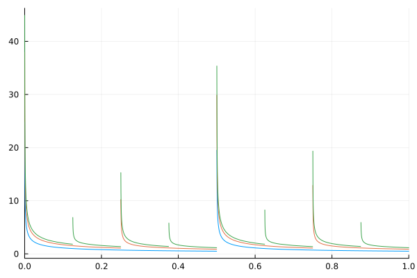
Figure 4. The first three (blue, orange, green) iterates of the iRB operator
when starting with the zero function.
The first iterate has two “spikes” at and and their number doubles with each iteration.
References
[1] M. F. Barnsley, Fractal Functions and Interpolation. Constr. Approx.2(1) (1986), 303–329.
[2] M.F. Barnsley, B. Harding, C. Vince, P. Viswanathan, Approximation of Rough Functions. J. Approx. Th.209 (2016), 23–43.
[3] M. F. Barnsley, M. Hegland, P. Massopust, Numerics and Fractals. Bull. Inst. Math. Acad. Sin. (N.S.)9(3) (2014), 389–430.
[4] T. Bedford, M. Dekking, M. Keane, Fractal Image Coding Techniques and Contraction Operators. Delft University of Technology Report (1992), 92–93.
[5] N. Dira, D. Levin, P. Massopust, Attractors of Trees of Maps and of Sequences of Maps Between Spaces and Applications to Dubdivision. J. Fixed Point Theory Appl.22(14) (2020), 1–24.
[6] S. Dubuc, Interpolation Fractale. In Fractal Geomety and Analysis, J. Bélais and S. Dubuc, eds., Kluwer Academic Publishers, Dordrecht, The Netherlands, 1989.
[7] J. E. Hutchinson, Fractals and Self-similarity. Indiana Univ. Math. J.30 (1981), 713–747.
[8] D. Kumar, A. K. B. Chand, P. Massopust, Approximation by Quantum Meyer-König-Zeller Fractal Functions. fractal and fractional6(12) (2022), 704.
[9] D. Levin, N. Dyn, P. Viswanathan, Non-stationary Versions of Fixed-Point Theory, with Applications to Fractals and Subdivision. J. Fixed Point Theory Appl.21 (2019), 1–25.
[10] Massopust, P.R. Fractal Functions, Fractal Surfaces, and Wavelets, 2nd ed., Academic Press: San Diego, USA, 2016.
[11] Massopust, P.R. Hypercomplex Iterated Function Systems. In: Current Trends in Analysis, its Applications and Computation.
Proceedings of the 12th ISAAC Congress, Aveiro, Portugal, Cereijeras, P.; Reissig, M.; Sabadini, I.; Toft, J. (eds.), Birkhäuser (2022), 589–598.
[12] P. Massopust, Fractal Interpolation: From Global to Local, to Nonstationary and Quaternionic. In: Frontiers of Fractal Analysis. Recent Advances and Challenges, CRC Press (2022), 24–48.
Birkhäuser, 2000.
[13] Navascués, M.A. Fractal Polynomial Interpolation. Z. Anal. Anwendungen24(2) (2005), 401–418.
[14] C. Serpa, J. Buescu, Constructive Solutions for Systems of Iterative Functional Equations. Constructive Approx.45(2) (2017), 273–299.
[15] C. Serpa, J. Buescu, Compatibility conditions for systems of iterative functional equations with non-trivial contact sets. Results Math.2 (2021), 1–19.
[16] T. Takagi, A Simple Example of a Continuous Function Without Derivative. Proc. Soc. Japan1 (1903), 176–177.