No Strings Attached: Boundaries and Defects in the Cubic Code
Abstract
Haah’s cubic code is the prototypical type-II fracton topological order. It instantiates the no string-like operator property that underlies the favorable scaling of its code distance and logical energy barrier. Previously, the cubic code was only explored in translation-invariant systems on infinite and periodic lattices. In these settings, the code distance scales superlinearly with the linear system size, while the number of logical qubits within the degenerate ground space exhibits a complicated functional dependence that undergoes large fluctuations within a linear envelope. Here, we extend the cubic code to systems with open boundary conditions and crystal lattice defects. We characterize the condensation of topological excitations in the vicinity of these boundaries and defects, finding that their inclusion can introduce local string-like operators and enhance the mobility of otherwise fractonic excitations. Despite this, we use these boundaries and defects to define new encodings where the number of logical qubits scales linearly without fluctuations, and the code distance scales superlinearly, with the linear system size. These include a subsystem encoding with open boundary conditions and a subspace encoding using lattice defects.
I Introduction
Quantum computers are required to operate effectively in the presence of errors and noisy operations Shor 1995; Steane 1996; Shor 1997; Preskill 1998. A primitive component of a quantum computer is the quantum hard drive: a system capable of safely storing quantum information for long periods of time. In comparison to leading approaches such as the surface code Kitaev 2003; Bravyi and Kitaev 1998, which require active procedures to continually detect and correct for errors Dennis et al. 2002, such a hard drive should be passively self-correcting. To this end, one can envision a system where quantum information is encoded in an energetic ground state and errors that corrupt this information are suppressed by macroscopic energy barriers Brown et al. 2016. Unfortunately, this behavior is impossible to achieve in many cases - such as the surface code - due to no-go theorems that prohibit self-correction in D systems Alicki et al. 2009; Bravyi and Terhal 2009; Bravyi et al. 2010a; Alicki et al. 2010; Yoshida 2011; Haah and Preskill 2012; Landon-Cardinal and Poulin 2013; Brown et al. 2016.
Fortunately, these theorems do not apply to higher spatial dimensions. Already in D there are topological codes with no string-like logical operators that have significantly better energy barriers than any D code Haah 2011; Haah 2013a. The earliest such example is Haah’s cubic code, which was found via a computational search Haah 2011. The cubic code model is part of a larger classification of unconventional topological phases of matter, known as fracton topological orders Chamon 2005; Bravyi et al. 2011; Haah 2011; Castelnovo and Chamon 2012; Kim 2012; Haah 2013a; Yoshida 2013; Vijay et al. 2015; Vijay et al. 2016; Williamson 2016. In this classification, topological codes with no string-like operators are called type-II fracton phases Vijay et al. 2016. As a type-II fracton phase, the cubic code only supports topological excitations that are completely immobile Haah 2011. When used as an error-correcting code, this immobility results in a code distance that scales superlinearly with the linear system size i.e., for , where is the number of lattice sites along one axis. Moreover, the minimum energy required to map between degenerate ground states via local operations - also known as the energy barrier - scales as Bravyi and Haah 2011. This energy barrier enables the cubic code to be partially self-correcting: its quantum memory time increases with the system size only up to a finite threshold that decreases with temperature Bravyi and Haah 2011. For comparison, the surface code in D has a memory time independent of system size. This property makes the cubic code a leading candidate for creating a quantum hard drive in D.
There are, however, additional features of the cubic code that are undesirable for applications to quantum error correction (QEC). The number of encoded qubits, , varies sporadically with the system size Haah 2013a (see Fig. 3). In an actual implementation, achieving a large , therefore, requires the system to be from a family of carefully chosen system sizes that have large jumps between them. Moreover, the model was formulated in a translation-invariant setting with periodic boundary conditions, arranging the physical qubits on a -torus. This topology is not feasible in a strictly local architecture.
Since the discovery of the cubic code, there has not yet been an examination into how the model’s topology or geometry may be modified, and how these modifications may affect its core characteristics, such as its no-string property or fracton topological order. A significant question is whether open boundary conditions or the inclusion of lattice defects affect the error-correcting properties of the code, either by improving or worsening them. In other codes, including such modifications has the potential to increase the number of encoded qubits or enable additional fault-tolerant quantum gates Bravyi and Kitaev 1998; Bombin 2010a; Brown et al. 2017; Bulmash and Iadecola 2019. However, in our setting, open boundary conditions and defects have the potential to introduce string-like operators and reduce the energy barrier for logical errors.
In this work, we characterize the properties of boundaries and defects in the cubic code, including their interactions with quasiparticle excitations. We investigate whether modifying the cubic code by introducing boundaries and defects can affect the scaling of the number of qubits while maintaining the superlinear code distance and favorable energy barrier of the periodic model. We approach this with a combination of analytic arguments, visualizations, and numerical computations. For the latter, we simulate lattices with up to approximately qubits, and assume a consistent extrapolation for larger systems.
I.1 Summary of Results
| Diagram | Notation | Name | Encoded Qubits () | Logical Weight |
![[Uncaptioned image]](2308.00138v1/boundary_pure.png) |
Only | - | ||
![[Uncaptioned image]](2308.00138v1/boundary_m.png) |
One | - | ||
![[Uncaptioned image]](2308.00138v1/boundary_mabc.png) |
One | - | ||
![[Uncaptioned image]](2308.00138v1/eeemem.png) |
Two | Constant, Superlinear | ||
![[Uncaptioned image]](2308.00138v1/memeee.png) |
Two | - | ||
![[Uncaptioned image]](2308.00138v1/meeeme.png) |
& | - | ||
![[Uncaptioned image]](2308.00138v1/boundary_tennis_1.png) |
Tennis ball 1 | Linear, Superlinear | ||
![[Uncaptioned image]](2308.00138v1/boundary_tennis_2.png) |
Tennis ball 2 | Constant, Superlinear | ||
![[Uncaptioned image]](2308.00138v1/boundary_tube.png) |
Tube | Constant, Linear, Superlinear | ||
![[Uncaptioned image]](2308.00138v1/boundary_half_B.png) |
Half-half 1 | - | ||
![[Uncaptioned image]](2308.00138v1/boundary_half_A.png) |
Half-half 2 | Constant, Superlinear | ||
![[Uncaptioned image]](2308.00138v1/boundary_trapezoidal.png) |
- | Triangular | Linear, Superlinear |
In this paper, we consider the construction of - or -type open boundaries normal to a crystallographic axis. These boundaries are gapped using plaquette stabilizers formed from truncated bulk and cube stabilizers respectively. Both cases exhibit two topologically distinct interactions with the fractonic excitations: -type boundaries on the negative-oriented faces of the lattice (and -type on the positive faces) condense single fractons. Conversely, -type positive faces (and -type negative faces) cause their corresponding fractons to gain a D mobility within diagonal subsystems along the surface. These boundary layers have a direct correspondence to the 6-6-6 color code Bombin and Martin-Delgado 2006.
Our results demonstrate that the no-string property of the closed cubic code model is not readily retained in the presence of open boundary conditions. Because of this, it is nontrivial to construct QEC codes with open boundary conditions that have the desired superlinear code distance. Table 1 summarizes the different configurations of open boundary conditions considered in this paper; none contain only logical operators with superlinear weight. Notably, however, the scaling of in all nontrivial cases is now a simple function of the linear system size that does not exhibit large fluctuations.
It is nevertheless possible to create a cubic code with open boundary conditions that has a superlinear distance. For this, we use the tennis ball 1 configuration from Table 1. In the corresponding code, logical and operators stretch between two boundaries in the and lattice directions respectively. There exist logical operators supported solely near the face, and operators near the face, that have linear weights. However, those further in the bulk have weight superlinear in . A subsystem code Bacon 2005; Poulin 2005 can be used to gauge out the logical qubits with either an or that can be supported near a boundary face - thus producing a code with superlinear distance.
Alternatively, with boundary conditions that are periodic in the direction only, we are able to construct stabilizer codes with simple linear scaling of and a superlinear code distance without resorting to subsystem codes. This result, along with other periodic boundary condition codes, is summarized in Table 2.
In addition to open boundary conditions, we study the inclusion of crystal lattice defects including vacancies, edge dislocations, and screw dislocations. Similar to the open boundaries, we focus on configurations that are aligned with the crystallographic axes. While modified stabilizer terms are provided for vacancies and edge dislocations, screw dislocations do not admit additional deformed stabilizers. We explore how condensation of fractons on defects affects the fracton mobility in the vicinity of these features. We propose several encodings using defects; configurations such as a pair of edge dislocations or multiple vacancies wrapped around a periodic boundary can form stabilizer code families with superlinear distances and a simple linear scaling of . These results are discussed in detail in Section VI.
To the best of our knowledge, this work constitutes the first exploration of boundaries and defects in a type-II fracton topological order. Our results demonstrate that introducing defects and boundaries into the cubic code leads to encodings with new features that could prove advantageous over encodings based on periodic boundary conditions. This includes encodings with a number of logical qubits that scales linearly with the linear system size, without fluctuations. This work is a first step towards a general theory of translation symmetry enrichment in type-II fracton topological orders.
| Notation | Encoded Qubits () | Code Distance |
| Eq. (6) | Superlinear | |
| Linear | ||
| Linear | ||
| 0 | - | |
| Linear | ||
| Superlinear∗ | ||
| 0 | - | |
| 0 | - | |
| 0 | - | |
| 0 | - | |
| 0 | - |
I.2 Outline of Paper
This paper is organized as follows: In Section II we present background on quantum error-correcting codes and outline the key properties of the cubic code. In Section III we characterize the open boundary conditions of the cubic code. In Section IV we discuss constructions of superlinear-distance codes. In Section V we characterize the inclusion of defects - vacancies, edge dislocations, and screw dislocations. In Section VI we discuss the use of defects to construct superlinear-distance codes. In Section VII we present our conclusions. The appendices include a discussion of further open and periodic boundary codes (Appendix A) and defect codes (Appendix B) considered in this study. A summary of all the potential boundary encodings is provided in Tables 1 and 2.
II Background
We begin with a brief review of quantum error-correcting codes and self-correcting quantum memories, before discussing the cubic code in particular.
II.1 Review of Quantum Error-Correcting Codes
A quantum error-correcting (QEC) code is a scheme to encode one or more quantum states within a higher-dimensional Hilbert space in order to provide the ability to detect and correct a class of errors. Arbitrary errors are generated by the algebra of single-qubit Pauli errors, spanned by the Pauli and operators
| (1) |
written in the computational basis corresponding to the two states of a physical qubit. One approach for constructing QEC codes is to employ the stabilizer formalism Calderbank et al. 1997; Gottesman 1998: Consider a system of physical qubits. We select a commuting collection of (tensor) products of Pauli operators and consider the stabilizer group that they generate. We require that , where is the identity operator. Quantum information is then encoded in the eigenvectors of the degenerate -eigenspace common to all elements of . That is, any physical measurement of the encoded state using returns a value. Importantly, single-qubit and operators anti-commute with some , thus mapping any encoded state out of the -eigenspace and producing a change in the measurement outcomes. This can be detected and corrected with appropriate QEC codes.
For a system with independent stabilizer generators and physical qubits, the degeneracy of the -eigenspace is . Equivalently, the number of encoded logical qubits that are protected from errors is .
An effective QEC code should have a large number of encoded qubits but also should make it difficult for errors to affect the encoded information. A logical operator, denoted as or , is an operator that commutes with all stabilizers, yet is not itself in the stabilizer group. In this way, logical operators act on the encoded states within the -subspace, changing the state of the logical qubit while not being detectable using stabilizer measurements. Effective QEC codes must therefore make it difficult for errors to create a logical operator (logical error). We quantify this difficulty in two ways: code distance and energy barriers.
Code Distance
Operators that act on encoded quantum states are only uniquely defined modulo multiplication by stabilizers. The weight of a logical operator - the number of single-qubit Pauli operators required to construct it - is therefore variable. The code distance is defined as the minimum weight operator that can create a logical error on the code, taking into account this multiplication by stabilizers.
Energy Barriers
Additionally, we can consider the physical qubits in a QEC code as forming a quantum condensed matter system, evolving under a Hamiltonian
| (2) |
where are spatially-local operators that generate the stabilizer group . Since the encoded states belong to the -eigenspace of all , they also correspond to the ground state (minimum energy state) of this system. Pauli errors then map an encoded state into the -eigenspace of some , thus increasing the energy. These flipped or excited stabilizers can be interpreted as the location of excitations or quasiparticles, with emergent behavior such as mobility, charge, and even braiding statistics. The ability of a code to correct against local errors is equivalent to the condition of topological order: the state of the system cannot be determined solely by local operations Wen 1990; Dennis et al. 2002; Bravyi et al. 2010b; Wen 2017.

The energy barrier of this system is then defined as the minimum energy that must be surpassed in order to create a logical error by sequentially applying single-qubit Pauli errors. Importantly, larger energy barriers will cause the evolution of the system to naturally suppress the creation of logical errors when at nonzero temperatures. That is, for an energy barrier , entropy change , temperature and Boltzmann constant , the time a system can remain in its encoded state (quantum memory time) scales approximately via the Arrhenius Law Roberts and Bartlett 2020
| (3) |
A self-correcting quantum memory at finite temperature is then defined as a QEC code where the lifetime grows without bound in the number of physical qubits, at sufficiently small nonzero temperature Bombin et al. 2013. A necessary condition for this, therefore, is that the energy barrier must grow with the system size. However, this behavior is impossible in all stabilizer codes formed by arranging the qubits in D and demanding the stabilizers be spatially local Alicki et al. 2009; Bravyi and Terhal 2009; Bravyi et al. 2010a; Alicki et al. 2010; Yoshida 2011; Haah and Preskill 2012; Landon-Cardinal and Poulin 2013; Brown et al. 2016. These no-go theorems do not necessarily apply to higher dimensions. In particular, self-correction is readily possible in D Dennis et al. 2002; Alicki et al. 2010. In D, there have been several attempts at creating such behavior Chesi et al. 2010; Yoshida 2011; Bombin et al. 2013; Becker et al. 2013; Brell 2016; Brown et al. 2016; Roberts and Bartlett 2020. One of the more promising candidates, and one of the only exactly-solvable candidates, is known as the cubic code.


| Charge | Created By | Excited Stabilizer | Color |
![[Uncaptioned image]](2308.00138v1/figures/bg/e_charge.png) | |||
![[Uncaptioned image]](2308.00138v1/figures/bg/m_charge.png) |
II.2 The Cubic Code
Initially proposed in Ref. Haah 2011, the cubic code is defined on a D simple cubic lattice with two qubits at each lattice site and periodically identified boundaries in all directions, forming a -torus. We use the notation to denote the operator acting on the two qubits at a particular lattice site, with the identity on all other qubits. The model has two kinds of stabilizer generators, both with support on a subset of the 16 qubits at the 8 vertices of a unit cube. These generators, referred to here as and , are shown in Fig. 1.
Pauli operators create tetrahedral excitation patterns in the neighboring stabilizers, highlighted in Fig. 2. Following the convention with the surface code, we denote these two types of excitations as and as in Table 3.
II.2.1 Lattice Symmetries
Noting the form of the stabilizers and their excitation patterns, there are three lattice symmetries of the cubic code relevant for discussions in this paper:
- 1.
-fold rotation about .
- 2.
Mirror symmetry about the plane normal to .
- 3.
The map combined with spatial inversion.
These symmetries are used to relate boundaries and defects with different orientations in later sections.
II.2.2 Encoding Properties
The defining property of the cubic code is that all its nontrivial topological quasiparticle excitations11 1 A nontrivial topological excitation is one that cannot be created locally. are fundamentally immobile fractons. This is equivalent to a property called “no string-like operators” Haah 2011. A string-like operator is any operator that creates two constant-sized regions of nontrivial topological excitations, separated by an arbitrary distance , with a weight that scales linearly with . In doing so, these operators incur a maximum energy cost that is independent of . Since such string-like operators do not exist in the cubic code, fractons cannot be moved large distances with constant energy. This immobility property is discussed further in Section II.2.3.
Importantly, this behavior results in a code distance that scales superlinearly with the linear system size (the number of sites in each lattice direction), and an energy barrier that scales logarithmically with . Although seemingly promising for use in self-correction, we also need to consider the effects of entropy. The entropy of a system is typically extensive, scaling polynomially with system size Bravyi and Haah 2011. As per Eq. (3), at finite temperature there will thus exist a given system size where increasing further results in a decrease to the lifetime, as entropic contributions overwhelm the system. This energy barrier is therefore enough to ensure only partial self-correction of the system Bravyi and Haah 2013. Nevertheless, it remains one of the only stabilizer codes to achieve even this behavior.
A key theorem for self-correcting quantum memories is that for there to be no string-like operators, the ground state degeneracy - or equivalently, the number of encoded qubits - in a D translation-invariant stabilizer code must depend on the system size Yoshida 2011. In the case of the cubic code, fluctuates significantly, bounded by , where we take a geometry with equal linear system size in and . For notation, we define
| (4) |
and
| (5) |
Using this, the exact empirical formula for is given by (see Ref. Haah 2011)
| (6) |
where we have written etc. for readability. This relationship is plotted in Fig. 3. A number-theoretic exact formula for is known for all but the formula is cumbersome to write down and not enlightening for our purposes Haah 2013b. Importantly, there is a strong dependence on the exact divisibility of ; changing can cause to fluctuate by several orders of magnitude. A guiding question for this work is whether the scaling can become a more consistent - ideally linear - function of by introducing open boundaries and lattice defects.
II.2.3 Fracton Mobility
As noted previously, there are no string-like operators through the bulk of the cubic code model. Consequently, the topological quasiparticle excitations are strictly immobile and cannot be moved through the lattice without incurring an additional energy penalty that scales with the distance, . There are three sufficient behaviors, presented below, that describe this generalized motion and form the basis of our arguments for code distance and energy barriers in later sections:

Fractal Operators
Firstly, fractons can be moved through the bulk of the model using operators arranged in the shape of fractal tetrahedra. Originally described in Ref. Haah 2011, the excitation patterns in Fig. 2 can be repeated in a fractal pattern to create increasingly larger separations of charge, as in Fig. 4. Notably, doing so requires multiple excitations to move outwards and it involves intermediary high-energy states. It was from this fractal behavior that the logarithmic energy barrier of the periodic cubic code was derived Bravyi and Haah 2011. Due to this fractal nature, this process can create excitations separated by a distance where for . This dependence on powers of contributes towards the sporadic scaling of logical qubits in the periodic cubic code: if the width of the lattice is not a power of , multiple smaller tetrahedra need to be combined in a nontrivial way, wrapping around the periodic boundary to annihilate all charges. This motivates the form of Eq. (5).

Cascade Operators
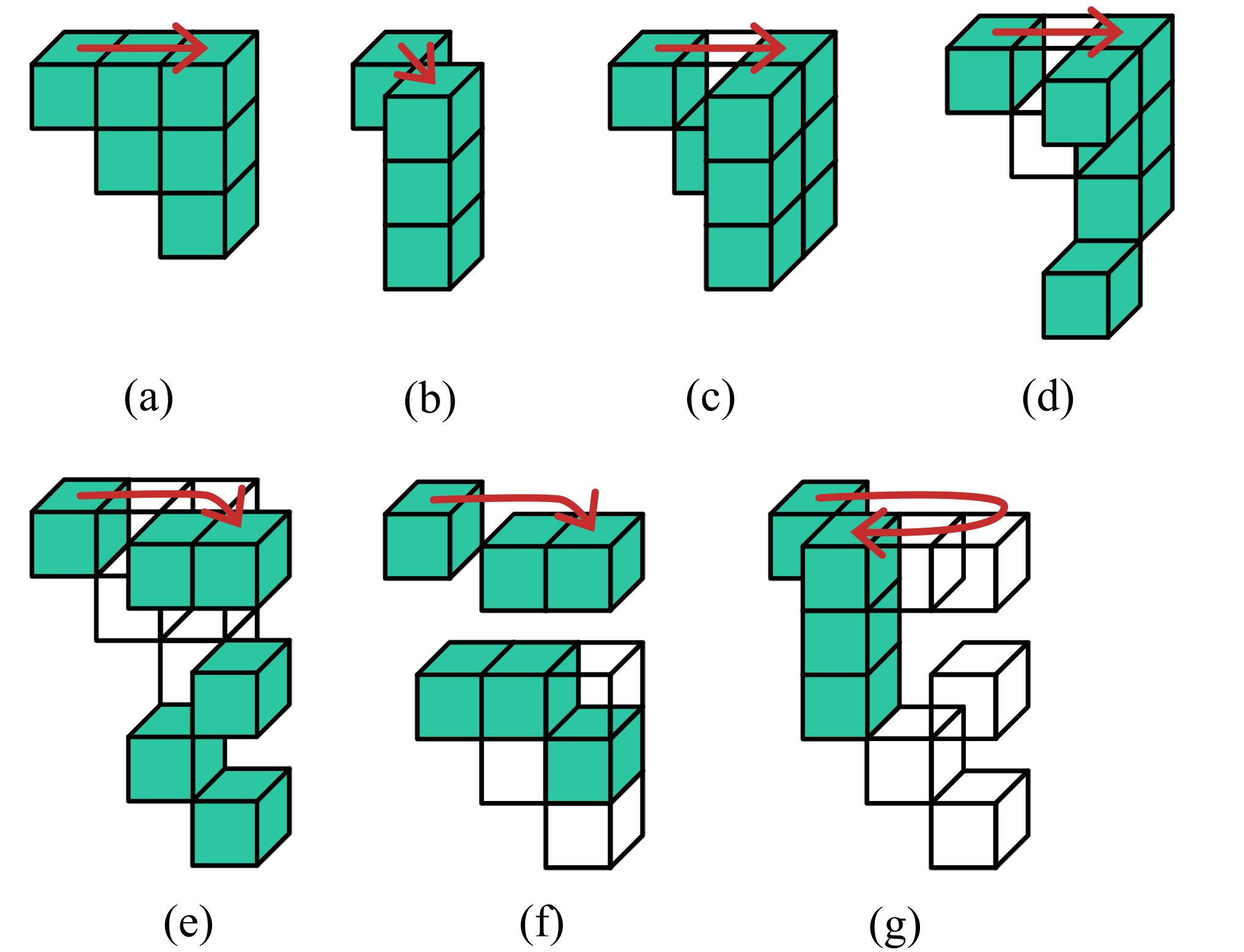
Secondly, excitations can be moved in a cascading operation (using the terminology from Ref. Bulmash and Iadecola 2019) that creates additional excitations at each step of the motion. To highlight this, we introduce three operators for and , as in Fig. 5. Using these operators repeatedly creates the cascading procedure shown in Fig. 6. Importantly, this process moves excitations through the bulk while requiring a Pauli weight that scales superlinearly with the distance , and creates additional excitations whose number scales linearly with . Numerically continuing this process for larger separations produces the results in Fig. 7.
Cage Operators
Thirdly, following the terminology of Ref. Bulmash and Iadecola 2019, a cage operator is a generalization of a Wilson loop that moves excitations around a closed path in the bulk, starting and ending from the vacuum state (ground state). This process is shown in Fig. 8. Notably, the locations of Pauli operators, as well as the intermediary excitations, occupy a cylindrical shell with the required height of the cylinder scaling linearly with the radius. When viewed from a particular direction ( in Fig. 8), this height can be compacted, leaving a D loop. Cage operators are particularly relevant for the discussion of defects in Section V.


II.3 Numerical Methods
In this work, we aim to derive formulae for the number of encoded qubits, , and the distance, , of variants of the cubic code with defects and modified boundary conditions. In general, however, it is difficult to rigorously derive exact equations for these properties. Therefore, we present motivating discussions, backed up by numerical computations of small system sizes where we can determine empirical formulae for these results. We then assume a consistent extrapolation for larger models.
To perform these calculations, the stabilizers in a system of qubits are represented by a binary vector in , with a corresponding to a Pauli or acting on a particular qubit Gottesman 1997. Commutation is a bilinear map between two such vectors, and finding nontrivial logical operators reduces to determining the kernel of this map when applied to the stabilizers. In this way, the number of logical operators (or equivalently, the ground-state degeneracy), and also examples of particular logical algebras, can be computed exactly for system sizes up to the order of qubits. By restricting to a subset of the physical qubits, we can also determine the properties of the support of these logical operators. These results form the basis for the conclusions drawn in the following sections. Code for these calculations is provided in Appendix C.3.
III Boundaries
In this section, we present and analyze formulations of the cubic code that incorporate combinations of open and periodic boundaries. By doing so, we identify the behavior of excitations on and near these boundaries, to inform the discussion of encoding properties in Section IV. We first consider isolated open boundaries in a semi-infinite system, before combining multiple boundaries via edges and vertices.
To characterize these boundaries, we introduce the following notation: Consider a rectangular prism centered at the origin of a Cartesian D coordinate system, with the terminating boundaries normal to the axes. In similar notation to Miller indices, we use ) to denote the boundary that forms across the positive side of the prism and ) to denote the boundary on the negative side. Additionally, define the sign of a boundary to be positive for , , and orientations and negative for , , and . An additional notation for specifying the types of stabilizers on these boundary faces is introduced in Section III.2. It is possible to consider other more general boundaries, such as those with Miller index . We present one such example in Appendix C.2 but will defer the systematic study of these boundaries to future work.
III.1 Semi-Infinite Boundaries
We first consider the family of semi-infinite systems, such as with a single terminating boundary corresponding to a crystallographic plane, and propose a set of maximal stabilizer generators to populate this boundary. There are two possible constructions of translation-invariant Hamiltonian terms that maintain the required commutation relations with both the neighboring bulk and boundary stabilizers. These correspond to truncated and operators, as shown in Fig. 9, where the bulk operator is continued outwards and all terms that lie beyond the system boundaries are ignored. We denote these single-face (or plaquette) operators as and .

Let -type denote a boundary Hamiltonian consisting of only , and -type for . More general configurations are possible, such as the triangular code in Table 1, but their properties can be explained solely by a discussion of the purely or -type boundaries.
Importantly, the orientation of a boundary affects its behavior. That is, the boundary Hamiltonian of an -type is not equivalent to that of an -type . We see this by observing the two inequivalent forms of truncated operators, as well as the symmetries noted in Section II.2.1.

III.1.1 Boundary Excitations
Various applications of Pauli operators on a boundary are shown in Fig. 10. When a single particle is able to be created or destroyed in isolation by a local operator in the vicinity of the boundary layer, we refer to this process as condensation. Of note, positive -type boundaries condense excitations, while negative -type boundaries condense excitations; we refer to these boundaries as and type respectively. However, on negative -type and positive -type boundaries, single excitations cannot be condensed. Instead, to describe their behavior, we introduce three new charges as subtypes of both the and : denoted and .
Consider a positive -type boundary in Fig. 11, where we striate the lattice to color squares along the diagonals as , or (such that an excitation on an -type square will have an charge, etc.). Importantly, a single (or an and an , for example) cannot be condensed in isolation. Instead, it gains D mobility along the boundary plane: charges are mobile along the diagonals via applications of , and can hop to other diagonals using a combination of . Equivalent results hold for and . This increased mobility resembles phenomena observed on the boundaries of type-I fracton models, like the X-cube model Vijay et al. 2016; Bulmash and Iadecola 2019.
Moreover, creates a topologically nontrivial composite of , , and excitations on the boundary. Motivated by these behaviors, we define the fusion rules
| (7) |
that describe how combinations of excitations can be created via local operators. We note that these are fusion rules. An analogous result holds for , and by substituting . Given this fundamentally different behavior to boundaries, we denote these positive -type boundaries as , and similarly for negative -type boundaries. A summary of the new boundary notation is given in Table 4.
For these charges to be considered topologically distinct, there must not be a local operator that can fuse , for example. By considering the action of and , this is trivially true using only operators with support on the boundary. Since such a fusion operator will create excitations only along the boundary, we complete the argument by using the cleaning process from Refs. Haah 2011; Dua et al. 2019a to reduce the support of any bulk operator to just terms on the boundary; we refer the reader there for a more detailed description. This argument holds when we consider operators stretching from the boundary into the bulk, as long as the operator does not have support on other boundaries (such as an opposing ). Therefore, it is valid to consider , , and as distinct charges with the boundary fusion properties above, if they are separated from additional boundaries by distances larger than the correlation length of the ground state.

| Boundary | Stabiliser | Sign | Color | Behavior |
| condenses | ||||
| Eq. (7) | ||||
| condenses | ||||
| Eq. (7) (for ) |
Due to the triplet fusion nature of these charges, these fusion rules bear a resemblance to that of the color code Bombin and Martin-Delgado 2006; Bombín 2015; Kesselring et al. 2018. In fact, the color code can be directly transformed into this D layer: Consider the hexagonal lattice of the 6-6-6 color code in Fig. 12, with a qubit at each lattice point (white circle). The stabilizers of this code are the product of or on all qubits of each hexagon. We begin the transformation by first overlaying a rhomboidal lattice such that its vertices lie between exactly two qubits , as shown in the inset. Note that acting on both qubits with , for example, excites the two adjacent stabilizers on the green hexagons. This is equivalent to exciting two squares along the diagonal of the cubic code’s using in Fig. 11. Moreover, acting with just excites the three adjacent red, green, and blue hexagons - equivalent to exciting , and using on the cubic code. Corresponding similarities also apply for operators acting on an boundary. We, therefore, have the following map relating excitations of the color code to excitations of the cubic code boundaries:
| (8) |
Notably, in the Heisenberg representation this transformation is equivalent to
acting on each pair with a CNOT gate, controlled on qubit Gottesman 1998. If we consider
the boundary on ) and on , then this
transformation directly maps the truncated boundary and stabilizers of the cubic code onto the and stabilizers of the color code. This property is discussed further
in Appendix C.2. It remains an open question as to how or whether this correspondence generalizes to the bulk stabilizers of the cubic code, and moreover for the other cubic codes proposed by Haah Haah 2011.
III.1.2 Periodic Behavior
Consider a lattice that is periodic in and occupies . Along the face we construct an boundary using stabilizers. If , then the diagonal striation (as in Fig. 11) of this boundary layer is self-consistent and we have distinct , and charges that are mobile within their D diagonal subspaces. That is, if an were to move around the periodic boundary, it would retain its charge. We can thus consider an operator that creates two out of the vacuum, hops one around the periodic boundary, and annihilates it with the other to create a logical operator - comparable to those in the D toric code, for example, Kitaev 2003. Due to the two unique charges (as by the fusion rules), these surface string operators define two independent logical operators along an or boundary. When , it can be checked that hopping an excitation three times around a boundary (to return it to its original labeling) produces the identity operator.
However, these string operators can be extended to additional layers beyond the boundary, creating operators that extend into the bulk while requiring longer periods. To describe this procedure, we consider each plane to be a generalization of the boundary layer. That is, acting with or at creates charges in both the and layers. Repeating the hopping process at to move an around the periodic boundary will remove all charges in that layer while introducing residual charge at . If this residual charge is trivial - that is, it is equivalent to the vacuum state up to the fusion operators in Eq. (7) - then the charge in that layer can also be cleaned away. Importantly, these processes only deposit residual charge in layers at smaller , not affecting layers that have already been cleaned of excitations. Since restricts any remaining charge from forming beyond the face itself, completing the process by annihilating charges at results in a (nontrivial) logical operator.
If this process were started instead at , then this cleaning can be continued downwards until either the topmost remaining layer has a nontrivial residual charge or all charges are annihilated or condensed into the boundary. In this way, nontrivial logical operators can be constructed at varying depths within the bulk, which wrap around the periodic boundary and iteratively clean layers of charge down to .
It can be shown (see Appendix C.1) that for a given lattice that is periodic in linear system size , the maximum number of layers that can be cleaned until a nontrivial residual charge is created is
| (9) |
using the notation in Eq. (5). This function is plotted in Fig. 13. Each layer introduces two additional nontrivial mutually commuting logical operators, giving
| (10) |
Note that if and the boundary is of type or , then since the maximum number of layers cannot fit in the given lattice. Incorporating this, we define the function
| (11) |
For rectangular lattices with , then we instead have
| (12) |
defined by the shortest path around the periodic boundary. As a result, if one of or is not a multiple of .
III.1.3 Translational-Symmetry Violations
If translational invariance is relaxed, there are additional possible commuting configurations of the boundary Hamiltonian. The commutation relation between neighboring plaquette terms is given in Fig 14. Notably, these relations allow for the construction of a natural diagonal commuting interface between operators, such as the configuration labeled triangular in Table 1.

As with the other boundaries discussed so far, each sector of the mixed boundary is associated with an or behavior. Due to this equivalence, this paper focuses on pure and boundary configurations.
III.2 Boundary Seams
As in Fig. 9, two adjacent boundaries can be joined along an edge, and three boundaries at a vertex. These features are required to construct the full codes discussed in Section IV.
Notably, the plaquette-plaquette commutation relations in Fig. 14 are equivalent for edge-plaquette commutation since geometrically, neighboring plaquettes only share support on at most two sites - identical to plaquettes. Given these constraints, we can thus specify a fully-gapped configuration for a finite prism such as in Table 1. To describe these configurations, the notation is used to specify the boundary type on each of the six lattice boundaries (see Fig. 15). For open boundaries, we use and as defined in Table 4, where the subscript is dropped for readability. Periodic boundaries are denoted by . It is assumed in each case that the edge and vertex stabilizers are chosen to create a maximally commuting stabilizer group of local operators (that is, where possible there are no local Pauli operators with support on a single plaquette, edge, or vertex that commute with all the stabilizers).
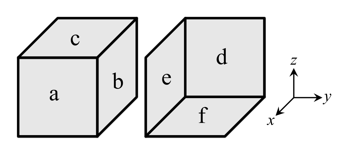
Using this notation, we can revisit the symmetries described in Section II.2.1:
- 1.
is equivalent to and .
- 2.
is equivalent to .
- 3.
is equivalent to with all swapped.
Combined, the first two symmetries imply that for , all permutations of produce equivalent codes, given that the same permutation is also applied to .
IV Superlinear-Distance Boundary Codes
A core motivation for this work is to maintain the partial self-correction of the cubic code, without the requirement of nonlocality to implement a -torus. Given the discussion in Section II, operators with superlinear weight (necessary for self-correction) arise when excitations cascade through the bulk of the lattice, while unwanted string-like operators appear near certain boundary configurations. Motivated by this, we thus consider codes that contain opposing boundaries and opposing boundaries. This specifies four of the six faces of the lattice, leaving (up to symmetries) a potential three unique configurations. In the following section, we highlight one such case, dubbed tennis ball 1, while the others are discussed in Appendix A.
IV.1 Tennis Ball 1
This configuration is constructed with and on the remaining two unspecified faces. For example, as shown in Table 1.
To construct logical operators, charges must cascade from and condense at using and , as shown in Fig. 16. If the excitations produced in the cascade cannot appear on the boundary, this procedure produces an operator with a weight superlinear in and an increasing energy barrier, since excitations must cascade through the bulk by a distance . However, if excitations can be produced on the boundary during the cascade, these excitations become mobile on the surface and can hop to the face using a string operator. Hence, any cascade that begins less than a distance of order from the boundary creates a string-like operator: the height is constant in , the weight is linear, and the energy cost is constant. An analogous argument holds for producing logical operators by cascading excitations; only cascades which begin a distance at least from the boundary produce logical operators with superlinear weight.


Notably, the logical operators extend in the direction and in the direction when cascading. Pairs of and must then anti-commute along their shared -plane. To determine the number of independent logical pairs, first note that using the long edge of the operators to move charges through the bulk is equivalent to the hopping operator in Fig. 11. We can then identify this cascading procedure with hopping an or charge from one boundary to the other, creating neighboring intermediary excitations that must also be hopped into a condensing boundary. In a similar argument to Section III.1.2, we, therefore, expect each layer to contribute encoded qubits. Since only one orientation, namely the planes, have opposing and -condensing boundaries - and therefore can support mutually anti-commuting pairs of both and operators - the scaling is thus expected to be . We confirm this by numerically computing the ground state degeneracy for small values of ; an example of the computed logical algebra cleaned into a single plane is shown in Fig. 17. This same analysis cannot be conducted with planes, for example, since these will have three adjoining -type boundaries and only one -type. As with the surface code, such a configuration does not support any nontrivial logical operators.
Notably, this scaling confirms the results in Ref. Dua et al. 2019b, where Dua et al. showed that the periodic cubic code can be interpreted as interwoven layers of toric code. Specifically, a model of linear system size is equivalent to copies of toric code, up to a unitary that is non-local in . When placed on open boundaries as done here, the corresponding surface codes should each contain one encoded qubit, thus giving total.
IV.2 Subsystem Codes
The presence of the string-like operators initially appears detrimental to the desired self-correcting behavior of the tennis ball code. However, we can still ensure a superlinear-distance encoding by using a subsystem code Bombin 2010b. By treating all logical qubits with linear distance as gauge qubits, the subsequent dressed logical operators should remain superlinear in weight. We argue this claim as follows:
First, note that the support of the bare superlinear-weight logical operators extends further in the direction than the bare linear-weight logical operators, by definition. This extra support includes a region in the bulk where the and pairs intersect and anti-commute. Since commutes with all stabilizers and all other operators apart from its pair, this anti-commutation relation must be maintained when multiplied with these other operators. Therefore, the product of bare superlinear and bare linear weight operators will always contain support on a region in the bulk of the lattice. This region is either entirely isolated from the boundary or extends to the boundary. In the former case, by the properties of the original cubic code, there are no string-like operators in the bulk of the lattice. For the latter, the operator now occupies a support that is larger than the original superlinear-weight support, which didn’t extend to the boundary. In both situations, the dressed operator must still have superlinear weight.
With tennis ball 1, we can, for example, label all logical operators that can be supported solely in or as ancillary. Computing the remaining ground state degeneracy numerically, the number of logical qubits is
| (13) |
The periodic scaling is a result of specifying discrete lattice points for the cut-off regions when may not divide .
It is therefore possible to modify the family of cubic codes such that we maintain the superlinear distance and partial self-correction while improving to be a simple linear function of , with only a constant-order periodic correction. Moreover, these codes do not require any periodic boundaries and are thus comparably more realistic for implementations in physical systems.
V Defects
Having presented the key properties of boundaries in the cubic code in the previous section, in the following section we similarly introduce and characterize three defect types: vacancies, edge dislocations, and screw dislocations. A discussion of their use in QEC codes is then provided in Section VI. Defects have been used in previous work to encode additional quantum information and to perform logical Clifford operations Bombin 2010a; Brown et al. 2013; Barkeshli et al. 2019; You 2019; Barkeshli et al. 2022; Krishna and Poulin 2020; Kesselring et al. 2018; Brown et al. 2017.
From a condensed matter perspective, defects are an important consideration when forming a complete understanding of a given phase of matter. For example, encircling a defect can induce a lattice translation. Since fractons are fundamentally immobile, this translation has the potential to cause nontrivial changes to the fracton topological order Manoj et al. 2021, such as in the form of increased mobility.
V.1 Vacancies
Vacancies, the removal of lattice sites (and qubits) within the bulk of the model, behave similarly to boundaries. Stabilizers obtained by truncating the operators acting on the vacant site still commute with all stabilizers away from the vacancy and with other truncated stabilizers of the same type. For simplicity, we consider only vacancies with single choices of truncated stabilizers, which we denote as and for and respectively. As with the boundaries, these results could be generalized to more complex constructions, such as orientations or combinations of and faces, in future works.
| Vacancy Type | Vacancy Boundary | Stabilizer | Boundary Sign | Behavior |
| condenses | ||||
| Eq. (7) | ||||
| condenses | ||||
| Eq. (7) (for ) |
We identify here three key ways in which bulk excitations interact with nearby vacancies, the first two of which are equivalent to the boundary interactions.
Firstly, fractons can condense into certain faces of and vacancies, just as with the exterior lattice boundaries. The analogous results to Table 4 are summarized in Table 5.
Secondly, if the vacancy extends in a particular direction, such as , mobilized charges on and faces of the vacancy are able to repeatedly hop along . If the vacancy extends around a lattice periodic in , and with , then an operator can create two out of the vacuum, hop one charge around the periodic boundary and annihilate it with the other. This is equivalent to the boundary behavior in Section III.1.2.
Finally, by employing a cage operator, fractons can encircle a vacancy. As described in Ref. Bulmash and Iadecola 2019 and Section II.2.3, these operators create a set of fractons out of the vacuum, separate them via a cascading procedure in two directions, before inverting the cascading operation to bring the excitations back together to annihilate - returning to the vacuum state. Such an operation in the bulk will typically be trivial, resulting in a product of stabilizers. However, the vacancy removes terms from the stabilizer group, causing a cage that encircles a vacancy to be potentially nontrivial.


V.2 Edge Dislocations
Edge dislocations in (3+1)D are analogous to those in the (2+1)D surface code Bombin 2010a, with the additional feature that the dislocation becomes a line extending into the third spatial dimension, as in Fig. 18. Along the dislocation line, we include trapezoidal prism stabilizer terms - known as twists in Refs. Bombin 2010a; Brown et al. 2013. Joining the twists are a region of slanted and operators (shown as white in Fig. 18) that naturally commute with the adjoining bulk stabilizers. For the twists themselves, however, there are only two choices of stabilizers: one from terms (denoted ) and another from (). These are provided in Fig. 19. Importantly, although and commute at the same location, adjacent and anti-commute. Constructing a gapped edge dislocation, therefore, requires taking either pure , pure , or and jointly on every second stabilizer (or some combination of the above). We could further consider a non-commuting, potentially gapless, Hamiltonian along the defect including all and terms with arbitrary weights. Due to the commutation relations, this Hamiltonian is seen to be equivalent to two copies of the quantum Ising model. We proceed to consider only the pure or defects, leaving more complicated configurations to future work.
As sketched in Fig. 18b, using a cage operator to propagate a fracton around a twist does not return the fracton to its original position; instead, the fracton moves by the Burgers vector of the dislocation. The once-immobile fractons thus gain limited mobility in the vicinity of a twist. This behavior has the potential to introduce nontrivial logical operators.
As with boundaries and vacancies, bulk excitations can condense onto particular twists. A twist condenses charges, while twist condenses . Since an edge dislocation is characterized by two twists, we denote, for example, to be a twist on the positive side of the pair, and on the negative side.
V.3 Screw Dislocations
The final defect type we consider is the screw dislocation, shown in Fig. 20. We label the screw as or by the handedness of the Burgers vector when traversing around the dislocation. Unlike the edge dislocation, the screw invokes a translation vector along the defect line itself. Importantly, this means that a fracton can continuously wind around the defect via cage operators while translating along the screw. Fractons thus gain 1D mobility in the vicinity of screw dislocations.
Unlike vacancies and twists, however, for the screw dislocations with a Burgers vector of considered here, there is no local operator supported on the dislocation line that commutes with the bulk stabilizers. Because of this, and screws have no inherent stabilizer and can condense both and excitations. Notably, this condensation behavior largely negates any change to the mobility of fractons near this screw, since individual and can be created or destroyed at any location along the defect, and thus become trivial.

VI Superlinear-Distance Defect Codes
Similar to the discussion of boundary codes in Section IV, in this section we examine how defects can be used with the cubic code to create QEC codes with superlinear distances. Further configurations without this property are discussed in Appendix B. Notably, although there are codes using screw dislocations with a superlinear distance, the number of encoded qubits there is constant. We therefore defer the discussion of screw-dislocation codes to Appendix B.3.

VI.1 Vacancy Encodings
Consider a lattice of size , where with the correlation length of the ground state, such that interactions with the boundaries are negligible. We also place periodic boundary conditions in the direction. Within this, there is an vacancy of width such that it extends around the periodic boundary. We expect that a single vacancy in this configuration does not modify the ground state degeneracy, since creating and annihilating on the same vacancy is trivial. Indeed, this result is confirmed by numerical computation, in all cases except when . As discussed in Section III.1.2, charges gain 1D mobility along a periodic boundary, producing additional logical operators. This gives a number of encoded qubits
| (14) |
where is defined in Eq. (11), with the factor of arising from the two unique string-like operators on the two boundaries of the vacancy. These logical operators all have a linear weight.
Once additional vacancies are introduced, however, additional logical operators arise. Numerically computing the ground state degeneracies, the number of encoded qubits scales with
| (15) |
where is the number of vacancies.
excitations can now cascade through the bulk from one vacancy to another, creating an logical operator with a weight that is superlinear in the vacancy separation (using the Manhattan distance). Each additional vacancy introduces an additional independent site for condensation, thus increasing . Moreover, since translation is a nontrivial action in the bulk of the model, performing the cascading procedure at different values of produces independent operators. This gives the dependence on .
On the other hand, the logical operators are formed from cages of excitations encircling a vacancy. Importantly, because these cage operators are moving charges through the bulk around the vacancy, these must also have a weight that scales superlinearly with the widths . If these widths were scaled with the separation between the vacancies, this encoding has the potential to be partially self-correcting (when ), while also supporting a number of encoded qubits that scale linearly in and the number of vacancies.
If the assumption of is relaxed, such as for an code with number of vacancies wrapping around the periodic boundary, we get two additional logical operators per , giving
| (16) |
in comparison to Eq. (15). This is because charges can now also cascade from the vacancies to a boundary.
Overall, this code is a notable improvement over the original cubic code model and does not require a subsystem code as in Section IV. Unlike vacancies in the surface code, there is also no significant trade-off between the code distance and the number of encoded qubits, since can be kept constant while using to increase , and using the dimensions (vacancy width and linear system size) to increase the code distance. However, this construction does require a topology with one periodic direction.
VI.2 Edge Dislocation Encodings
A single edge dislocation in the bulk, far from any boundary, encodes no additional logical qubits.
However, more appealing behavior arises using multiple edge dislocations. Consider two dislocations, in Fig. 21a, each of height in the direction and separated by perpendicular distance in the direction. The dislocation line extends along . Numerically computing the ground space degeneracy yields
| (17) |
for some additional constant arising depending on the exact choice of twist stabilizers, , and .
Effectively, these logical operators consist of movement of and excitations around and between two of the four twists, as in Fig. 21a. Importantly, because these cage operators are moving charges through the bulk, the prohibition of string-like operators means that the width of the support in the direction must increase with and . This result is confirmed by numerically computing the minimum width that supports logical operators as we scale in Fig. 21b. Slight variations in the widths are due to the particulars for constructing the operators around the twists. However, in all cases, we observe an overall linear trend.
If the analysis above is repeated except with open or periodic boundary conditions in , we observe the same scaling as in Eq. (17). There is an additional, constant number of logical operators that have support solely on a single twist and are string-like in the direction. Unlike the case with vacancies, these operators remain even if . As with the case for tennis ball 1, considering a subsystem code to ignore these extra logical operators may be sufficient to ensure the dressed code has a superlinear distance as and are increased. A rigorous proof of this solution is deferred to future works.
As with periodic vacancies, pairs of twists provide a promising approach to improve the cubic code: maintaining the desirable code distance while encoding a number of qubits that scales linearly with .
VII Conclusion
In this work, we have presented a systematic study of open boundaries and defects in Haah’s cubic code. We focused on planar -like boundaries normal to the crystallographic axes and constructed - and -type open boundary conditions using truncated plaquette, edge and vertex stabilizer terms. The interaction of these boundaries with fractonic topological excitations depends intrinsically on their orientation: -type negative faces and -type positive faces condense single fractons of the respective type, while the opposing faces lead to increased fracton mobility within their vicinity. These otherwise fractonic excitations become mobile within a D diagonal subsystem along the surface. This implies that the fundamental no string-like operator property of the original cubic code is violated in the vicinity of these boundaries.
Similar behavior was observed in the vicinity of vacancies, edge dislocations, and screw dislocations: patterns of fracton condensation that lead to increased mobility were seen to depend on the orientation and stabilizer type of each defect. The nontrivial action of translation symmetry on a type-II fracton topological phase means that encircling a dislocation defect with a cage operator can also lead to increased topological excitation mobility. We found that dislocation defect encodings were therefore able to support additional forms of logical operators that do not appear for encodings constructed from boundaries and vacancies.
The cubic code is known to form a partially self-correcting quantum memory on periodic boundary conditions Bravyi and Haah 2013. The absence of any string-like logical operator is essential to enable such a quantum memory Haah 2011. With this in mind, we aimed to determine if it is possible to retain the superlinear distance of the original cubic code model while making the number of encoded qubits scale as a simple linear function of the linear system size, without sporadic fluctuation. We have shown that it is possible to achieve this using a combination of open and periodic boundaries, vacancies, and defects, despite the no string-like operator property potentially being lost when translation-invariance is violated by the introduction of defects. For cubic codes with open boundary conditions - which are typically easier to realize in a physical implementation - it is possible to achieve a superlinear code distance by restricting the encoded states to a subsystem, with all dressed logical operators maintaining a weight that scales superlinearly with the linear system size. We have shown this to be possible with the tennis ball 1 code construction. It is an open question whether this can be generalized to other open boundary condition codes, such as those in Appendix A. Our results also focused on planar -like boundaries; it remains an open question as to whether alternate constructions such as boundaries yield fundamentally different behavior.
We showed that emergent D topological order arises on certain open boundary conditions, supporting particles with increased mobility. Interestingly, this phase can be unitarily transformed into the 6-6-6 color code. We leave a further investigation of this correspondence, such as how it extends into the bulk, to future research. Similarly, it would be interesting to relate the bulk cubic code defects to defects of the color code Kesselring et al. 2018 on the boundary. Presumably, the emergent color code on the boundary has an associated non-invertible anomaly Ji and Wen 2019 which is a property of the type-II fracton bulk phase. Understanding the nature of the surface topological order could uncover further insights into type-II fracton topological order via a bulk-boundary correspondence.
In this work we have only explored Pauli- or type boundaries of the cubic code, rather than more complicated mixed or twisted boundary conditions. We suspect that such boundary conditions exist and are inequivalent to those we have studied. Our reasoning uses the construction of twisted boundaries via gauging symmetry-protected topological (SPT) domain walls Yoshida 2017. For the cubic code, this allows a construction of boundaries via the gauging duality to a 3D fractal Ising model Vijay et al. 2016; Williamson 2016. For one type of boundary condition of the fractal Ising model, the symmetry action on the boundary is simply the action of the bulk fractal symmetry restricted to the boundary plane. This symmetry action on the boundary appears to also be a fractal of the form considered in Ref. Devakul 2019. Following Ref. Devakul 2019, one can consider stacking the fractal Ising model with a reflected copy of itself such that the resulting boundary fractal symmetry supports a nontrivial fractal SPT phase. We can then twist the boundary condition by the associated SPT entangler and gauge the resulting model to obtain a twisted boundary condition of a cubic code stacked with a reflected cubic code. We leave the detailed study and classification of such twisted boundary conditions to future work. We anticipate that existing constructions of type-II fracton models from layers of fractal SPTs may prove advantageous for this study Williamson and Devakul 2021.
We now highlight several further directions for future consideration. It remains to be seen how the results in this paper can be generalized to other type-II fracton topological phases, such as the additional codes introduced in Ref. Haah 2011 or the fractal spin liquid codes Yoshida 2013. It would be interesting to relate defects in the latter codes to known defects in D topological codes via the fractalization procedure of Ref. Devakul and Williamson 2021. Our work, together with previous work on type-I fracton phases Bulmash and Iadecola 2019, raises the question of developing a general theory of boundaries and defects for fracton topological orders. A promising approach to this is the inclusion of conventional topological boundaries and defects into the topological defect network framework for fracton topological order Slagle et al. 2019; Aasen et al. 2020; Song et al. 2023a. Another interesting open question is the development of a notion of Lagrangian algebra objects Levin 2013; Beigi et al. 2011; Kitaev and Kong 2012; Kong 2014 for fracton topological orders that can be used to classify possible gapped boundaries in relation to fracton braiding statistics Pai and Hermele 2019; Song et al. 2023b. A further challenge is the extension of these concepts to nonabelian fracton models Vijay and Fu 2017; Prem et al. 2019; Song et al. 2019; Prem and Williamson 2019; Bulmash and Barkeshli 2019; Williamson and Cheng 2023; Sullivan et al. 2021; Tantivasadakarn et al. 2021.
Our work leaves open the question of superlinear code distances for subspace stabilizer encodings in type-II codes with open boundary conditions. It could be interesting to search for bounds on the best achievable parameters for a topological subspace stabilizer code with open boundary conditions in D. Proving rigorous lower bounds on the code distance and energy barriers, as well as modifying the decoding algorithms from Ref. Haah 2013a and Brown and Williamson 2020 in the presence of boundaries and defects, would allow us to make a more definitive judgment on the feasibility of these codes as self-correcting quantum memories. It would also be useful to consider how lattice defects can be braided to produce Clifford gate sets, such as with the surface code Bombin 2010a. Another open direction for future work is calculating the fusion of multiple twist and screw dislocations to create defects with larger Burgers vectors, and the relationship between braiding and condensations on these defects. This raises the challenge of developing a theory of translation symmetry enrichment for fracton topological orders, extending the D results of Ref. Barkeshli et al. 2019. This is a promising lens through which to understand the general structure of fracton topological orders on crystal lattices. We remark that the possible phenomena exhibited by known fracton models reveal a far richer theory than the two-dimensional analog Else and Thorngren 2019. In particular, a general theory should capture the interplay between subgroups of translation symmetry and bifurcating entanglement-renormalization group flows satisfied by fracton topological orders including the cubic code Evenbly and Vidal 2014; Haah 2014; Shirley et al. 2018; Dua et al. 2019c.
Acknowledgements.
The authors acknowledge fruitful collaboration with Tom Iadecola and Meng Cheng during the early stages of this work. AD and DB are supported by the Simons Collaboration on Ultra-Quantum Matter, which is a grant from the Simons Foundation (651438, AD; 651440, DB). AD is also supported by the Institute for Quantum Information and Matter, an NSF Physics Frontiers Center (PHY-1733907). ACD is supported by the Australian Research Council Centre of Excellence for Engineered Quantum Systems (EQUS, CE170100009). DW is supported by the Australian Research Council Discovery Early Career Research Award (DE220100625).References
- Shor (1995) P. W. Shor, Scheme for reducing decoherence in quantum computer memory, Physical Review A 52, R2493 (1995).
- Steane (1996) A. M. Steane, Error Correcting Codes in Quantum Theory, Physical Review Letters 77, 793 (1996).
- Shor (1997) P. W. Shor, Fault-tolerant quantum computation (1997), arxiv:quant-ph/9605011 .
- Preskill (1998) J. Preskill, Fault-Tolerant Quantum Computation, in Introduction to Quantum Computation and Information (WORLD SCIENTIFIC, 1998) pp. 213–269.
- Kitaev (2003) A. Y. Kitaev, Fault-tolerant quantum computation by anyons, Annals of Physics 303, 2 (2003), arxiv:quant-ph/9707021 .
- Bravyi and Kitaev (1998) S. B. Bravyi and A. Y. Kitaev, Quantum codes on a lattice with boundary, arXiv:quant-ph/9811052 (1998), arxiv:quant-ph/9811052 .
- Dennis et al. (2002) E. Dennis, A. Kitaev, A. Landahl, and J. Preskill, Topological quantum memory, Journal of Mathematical Physics 43, 4452 (2002), arxiv:quant-ph/0110143 .
- Brown et al. (2016) B. J. Brown, D. Loss, J. K. Pachos, C. N. Self, and J. R. Wootton, Quantum memories at finite temperature, Reviews of Modern Physics 88, 045005 (2016), arxiv:1411.6643 [cond-mat, physics:quant-ph] .
- Alicki et al. (2009) R. Alicki, M. Fannes, and M. Horodecki, On thermalization in Kitaev’s 2D model, Journal of Physics A: Mathematical and Theoretical 42, 065303 (2009).
- Bravyi and Terhal (2009) S. Bravyi and B. Terhal, A no-go theorem for a two-dimensional self-correcting quantum memory based on stabilizer codes, New Journal of Physics 11, 043029 (2009).
- Bravyi et al. (2010a) S. Bravyi, D. Poulin, and B. Terhal, Tradeoffs for Reliable Quantum Information Storage in 2D Systems, Physical Review Letters 104, 050503 (2010a).
- Alicki et al. (2010) R. Alicki, M. Horodecki, P. Horodecki, and R. Horodecki, On Thermal Stability of Topological Qubit in Kitaev’s 4D Model, Open Systems & Information Dynamics 17, 1 (2010).
- Yoshida (2011) B. Yoshida, Feasibility of self-correcting quantum memory and thermal stability of topological order, Annals of Physics 326, 2566 (2011).
- Haah and Preskill (2012) J. Haah and J. Preskill, Logical-operator tradeoff for local quantum codes, Physical Review A 86, 032308 (2012).
- Landon-Cardinal and Poulin (2013) O. Landon-Cardinal and D. Poulin, Local Topological Order Inhibits Thermal Stability in 2D, Physical Review Letters 110, 090502 (2013).
- Haah (2011) J. Haah, Local stabilizer codes in three dimensions without string logical operators, Physical Review A 83, 042330 (2011), arxiv:1101.1962 .
- Haah (2013a) J. Haah, Lattice quantum codes and exotic topological phases of matter, arXiv:1305.6973 [quant-ph] (2013a), arxiv:1305.6973 [quant-ph] .
- Chamon (2005) C. Chamon, Quantum Glassiness in Strongly Correlated Clean Systems: An Example of Topological Overprotection, Physical Review Letters 94, 040402 (2005).
- Bravyi et al. (2011) S. Bravyi, B. Leemhuis, and B. M. Terhal, Topological order in an exactly solvable 3D spin model, Annals of Physics 326, 839 (2011).
- Castelnovo and Chamon (2012) C. Castelnovo and C. Chamon, Topological quantum glassiness, Philosophical Magazine 92, 304 (2012).
- Kim (2012) I. H. Kim, D local qupit quantum code without string logical operator, arXiv , 9 (2012), arXiv:1202.0052 .
- Yoshida (2013) B. Yoshida, Exotic topological order in fractal spin liquids, Physical Review B 88, 125122 (2013), arxiv:1302.6248 .
- Vijay et al. (2015) S. Vijay, J. Haah, and L. Fu, A new kind of topological quantum order: A dimensional hierarchy of quasiparticles built from stationary excitations, Physical Review B 92, 235136 (2015).
- Vijay et al. (2016) S. Vijay, J. Haah, and L. Fu, Fracton Topological Order, Generalized Lattice Gauge Theory and Duality, Physical Review B 94, 235157 (2016), arxiv:1603.04442 .
- Williamson (2016) D. J. Williamson, Fractal symmetries: Ungauging the cubic code, Physical Review B 94, 155128 (2016), arxiv:1603.05182 [cond-mat, physics:hep-lat, physics:quant-ph] .
- Bravyi and Haah (2011) S. Bravyi and J. Haah, On the energy landscape of 3D spin Hamiltonians with topological order, Physical Review Letters 107, 150504 (2011), arxiv:1105.4159 .
- Bombin (2010a) H. Bombin, Topological Order with a Twist: Ising Anyons from an Abelian Model, Physical Review Letters 105, 030403 (2010a), arxiv:1004.1838 .
- Brown et al. (2017) B. J. Brown, K. Laubscher, M. S. Kesselring, and J. R. Wootton, Poking holes and cutting corners to achieve Clifford gates with the surface code, Physical Review X 7, 021029 (2017), arxiv:1609.04673 [cond-mat, physics:quant-ph] .
- Bulmash and Iadecola (2019) D. Bulmash and T. Iadecola, Braiding and Gapped Boundaries in Fracton Topological Phases, Physical Review B 99, 125132 (2019), arxiv:1810.00012 .
- Bombin and Martin-Delgado (2006) H. Bombin and M. A. Martin-Delgado, Topological Quantum Distillation, Physical Review Letters 97, 180501 (2006).
- Bacon (2005) D. Bacon, Operator Quantum Error Correcting Subsystems for Self-Correcting Quantum Memories, Physical Review A - Atomic, Molecular, and Optical Physics 73, 10.1103/PhysRevA.73.012340 (2005), arXiv:0506023 [quant-ph] .
- Poulin (2005) D. Poulin, Stabilizer Formalism for Operator Quantum Error Correction, Physical Review Letters 95, 10.1103/PhysRevLett.95.230504 (2005), arXiv:0508131 [quant-ph] .
- Calderbank et al. (1997) A. R. Calderbank, E. M. Rains, P. W. Shor, and N. J. A. Sloane, Quantum Error Correction and Orthogonal Geometry, Physical Review Letters 78, 405 (1997).
- Gottesman (1998) D. Gottesman, The Heisenberg Representation of Quantum Computers, arXiv:quant-ph/9807006 (1998), arxiv:quant-ph/9807006 .
- Wen (1990) X. G. Wen, Topological Orders in Rigid States, International Journal of Modern Physics B 04, 239 (1990).
- Bravyi et al. (2010b) S. Bravyi, M. B. Hastings, and S. Michalakis, Topological quantum order: Stability under local perturbations, Journal of Mathematical Physics 51, 093512 (2010b).
- Wen (2017) X.-G. Wen, Colloquium: Zoo of quantum-topological phases of matter, Reviews of Modern Physics 89, 041004 (2017).
- Roberts and Bartlett (2020) S. Roberts and S. D. Bartlett, Symmetry-Protected Self-Correcting Quantum Memories, Physical Review X 10, 031041 (2020).
- Bombin et al. (2013) H. Bombin, R. W. Chhajlany, M. Horodecki, and M. A. Martin-Delgado, Self-correcting quantum computers, New Journal of Physics 15, 055023 (2013).
- Chesi et al. (2010) S. Chesi, B. Röthlisberger, and D. Loss, Self-correcting quantum memory in a thermal environment, Physical Review A 82, 022305 (2010).
- Becker et al. (2013) D. Becker, T. Tanamoto, A. Hutter, F. L. Pedrocchi, and D. Loss, Dynamic generation of topologically protected self-correcting quantum memory, Physical Review A 87, 042340 (2013).
- Brell (2016) C. G. Brell, A proposal for self-correcting stabilizer quantum memories in 3 dimensions (or slightly less), New Journal of Physics 18, 013050 (2016).
- Bravyi and Haah (2013) S. Bravyi and J. Haah, Analytic and numerical demonstration of quantum self-correction in the 3D Cubic Code, Physical Review Letters 111, 200501 (2013), arxiv:1112.3252 .
- Haah (2013b) J. Haah, Commuting Pauli Hamiltonians as Maps between Free Modules, Communications in Mathematical Physics 324, 351 (2013b).
- Gottesman (1997) D. E. Gottesman, Stabilizer Codes and Quantum Error Correction, Ph.D. thesis, California Institute of Technology (1997).
- Dua et al. (2019a) A. Dua, I. H. Kim, M. Cheng, and D. J. Williamson, Sorting topological stabilizer models in three dimensions, Physical Review B 100, 155137 (2019a), arxiv:1908.08049 .
- Bombín (2015) H. Bombín, Gauge color codes: Optimal transversal gates and gauge fixing in topological stabilizer codes, New Journal of Physics 17, 083002 (2015).
- Kesselring et al. (2018) M. S. Kesselring, F. Pastawski, J. Eisert, and B. J. Brown, The boundaries and twist defects of the color code and their applications to topological quantum computation, Quantum 2, 101 (2018).
- Dua et al. (2019b) A. Dua, D. J. Williamson, J. Haah, and M. Cheng, Compactifying fracton stabilizer models, Physical Review B 99, 245135 (2019b).
- Bombin (2010b) H. Bombin, Topological subsystem codes, Physical Review A 81, 032301 (2010b).
- Brown et al. (2013) B. J. Brown, S. D. Bartlett, A. C. Doherty, and S. D. Barrett, Topological Entanglement Entropy with a Twist, Physical Review Letters 111, 220402 (2013), arxiv:1303.4455 .
- Barkeshli et al. (2019) M. Barkeshli, P. Bonderson, M. Cheng, and Z. Wang, Symmetry fractionalization, defects, and gauging of topological phases, Physical Review B 100, 10.1103/PhysRevB.100.115147 (2019), arXiv:1410.4540 .
- You (2019) Y. You, Non-Abelian defects in fracton phases of matter, Physical Review B 100, 075148 (2019).
- Barkeshli et al. (2022) M. Barkeshli, Y.-A. Chen, S.-J. Huang, R. Kobayashi, N. Tantivasadakarn, and G. Zhu, Codimension 2 defects and higher symmetries in (3+1)D topological phases (2022), arxiv:2208.07367 [cond-mat, physics:hep-th, physics:math-ph, physics:quant-ph] .
- Krishna and Poulin (2020) A. Krishna and D. Poulin, Topological wormholes: Nonlocal defects on the toric code, Physical Review Research 2, 023116 (2020).
- Manoj et al. (2021) N. Manoj, K. Slagle, W. Shirley, and X. Chen, Screw dislocations in the X-cube fracton model, SciPost Physics 10, 094 (2021), arxiv:2012.07263 .
- Ji and Wen (2019) W. Ji and X. G. Wen, Noninvertible anomalies and mapping-class-group transformation of anomalous partition functions, Physical Review Research 1, 10.1103/PhysRevResearch.1.033054 (2019), arXiv:1905.13279 .
- Yoshida (2017) B. Yoshida, Gapped boundaries, group cohomology and fault-tolerant logical gates, Annals of Physics 377, 387 (2017), arXiv:1509.03626 .
- Devakul (2019) T. Devakul, Classifying local fractal subsystem symmetry-protected topological phases, Physical Review B 99, 235131 (2019).
- Williamson and Devakul (2021) D. J. Williamson and T. Devakul, Type-II fractons from coupled spin chains and layers, Physical Review B 103, 155140 (2021).
- Devakul and Williamson (2021) T. Devakul and D. J. Williamson, Fractalizing quantum codes, Quantum 5, 438 (2021).
- Slagle et al. (2019) K. Slagle, D. Aasen, and D. Williamson, Foliated field theory and string-membrane-net condensation picture of fracton order, SciPost Physics 6, 10.21468/scipostphys.6.4.043 (2019), arXiv:1812.01613 .
- Aasen et al. (2020) D. Aasen, D. Bulmash, A. Prem, K. Slagle, and D. J. Williamson, Topological defect networks for fractons of all types, Physical Review Research 2, 043165 (2020).
- Song et al. (2023a) Z. Song, A. Dua, W. Shirley, and D. J. Williamson, Topological Defect Network Representations of Fracton Stabilizer Codes, PRX Quantum 4, 010304 (2023a).
- Levin (2013) M. Levin, Protected Edge Modes without Symmetry, Physical Review X 3, 021009 (2013).
- Beigi et al. (2011) S. Beigi, P. W. Shor, and D. Whalen, The Quantum Double Model with Boundary: Condensations and Symmetries, Communications in Mathematical Physics 306, 663 (2011), arXiv:1006.5479 .
- Kitaev and Kong (2012) A. Kitaev and L. Kong, Models for Gapped Boundaries and Domain Walls, Communications in Mathematical Physics 313, 351 (2012), arXiv:1104.5047 .
- Kong (2014) L. Kong, Anyon condensation and tensor categories, Nuclear Physics B 886, 436 (2014), arXiv:1307.8244 .
- Pai and Hermele (2019) S. Pai and M. Hermele, Fracton fusion and statistics, Physical Review B 100, 10.1103/PhysRevB.100.195136 (2019), arXiv:1903.11625 .
- Song et al. (2023b) H. Song, N. Tantivasadakarn, W. Shirley, and M. Hermele, Fracton Self-Statistics, (2023b), arXiv:2304.00028 .
- Vijay and Fu (2017) S. Vijay and L. Fu, A Generalization of Non-Abelian Anyons in Three Dimensions, (2017), arXiv:1706.07070 .
- Prem et al. (2019) A. Prem, S. J. Huang, H. Song, and M. Hermele, Cage-Net Fracton Models, Physical Review X 9, 10.1103/PhysRevX.9.021010 (2019), arXiv:1806.04687 .
- Song et al. (2019) H. Song, A. Prem, S. J. Huang, and M. A. Martin-Delgado, Twisted fracton models in three dimensions, Physical Review B 99, 10.1103/PhysRevB.99.155118 (2019), arXiv:1805.06899 .
- Prem and Williamson (2019) A. Prem and D. Williamson, Gauging permutation symmetries as a route to non-Abelian fractons, SciPost Physics 7, 068 (2019), arXiv:1905.06309 .
- Bulmash and Barkeshli (2019) D. Bulmash and M. Barkeshli, Gauging fractons: Immobile non-Abelian quasiparticles, fractals, and position-dependent degeneracies, Physical Review B 100, 10.1103/PhysRevB.100.155146 (2019), arXiv:1905.05771 .
- Williamson and Cheng (2023) D. J. Williamson and M. Cheng, Designer non-Abelian fractons from topological layers, Physical Review B 107, 10.1103/PhysRevB.107.035103 (2023), arXiv:2004.07251 .
- Sullivan et al. (2021) J. Sullivan, T. Iadecola, and D. J. Williamson, Planar p-string condensation: Chiral fracton phases from fractional quantum Hall layers and beyond, Physical Review B 103, 10.1103/PhysRevB.103.205301 (2021), arXiv:2010.15127 .
- Tantivasadakarn et al. (2021) N. Tantivasadakarn, W. Ji, and S. Vijay, Non-Abelian hybrid fracton orders, Physical Review B 104, 10.1103/PhysRevB.104.115117 (2021), arXiv:2106.03842 .
- Brown and Williamson (2020) B. J. Brown and D. J. Williamson, Parallelized quantum error correction with fracton topological codes, Physical Review Research 2, 013303 (2020), arxiv:1901.08061 .
- Else and Thorngren (2019) D. V. Else and R. Thorngren, Crystalline topological phases as defect networks, Physical Review B 99, 10.1103/PhysRevB.99.115116 (2019), arXiv:1810.10539 .
- Evenbly and Vidal (2014) G. Evenbly and G. Vidal, Class of highly entangled many-body states that can be efficiently simulated, Physical Review Letters 112, 240502 (2014), arXiv:1210.1895 .
- Haah (2014) J. Haah, Bifurcation in entanglement renormalization group flow of a gapped spin model, Physical Review B - Condensed Matter and Materials Physics 89, 75119 (2014), arXiv:1310.4507 .
- Shirley et al. (2018) W. Shirley, K. Slagle, Z. Wang, and X. Chen, Fracton Models on General Three-Dimensional Manifolds, Physical Review X 8, 10.1103/PhysRevX.8.031051 (2018), arXiv:1712.05892 .
- Dua et al. (2019c) A. Dua, P. Sarkar, D. J. Williamson, and M. Cheng, Bifurcating entanglement-renormalization group flows of fracton stabilizer models, PHYSICAL REVIEW RESEARCH 2, 33021 (2019c), arXiv:1909.12304 .
- Kitaev (1997) A. Yu. Kitaev, Quantum Error Correction with Imperfect Gates, in Quantum Communication, Computing, and Measurement, edited by O. Hirota, A. S. Holevo, and C. M. Caves (Springer US, Boston, MA, 1997) pp. 181–188.
- Alloul et al. (2009) H. Alloul, J. Bobroff, M. Gabay, and P. J. Hirschfeld, Defects in correlated metals and superconductors, Reviews of Modern Physics 81, 45 (2009).
Appendix A Additional Boundary Codes
Configurations such as tennis ball 1, vacancies around periodic boundaries, and pairs of twists have the potential to be partially self-correcting, while having a number of encoded qubits that scales linearly in some macroscopic quantity. However, this behavior is not true for the majority of other configurations. In this section, we present the remaining results from a systematic study of all boundary configurations (up to symmetries, and with pure -like planar boundaries). A discussion on defects is provided in Appendix B.
We first consider models with open boundary conditions on all six faces, before also addressing combinations with periodic boundaries. We perform a systematic search over all configurations, up to symmetries, and their key results are summarized in Tables 1 and 2.
A.1 Simple Cases
Following the construction in Section III, we first verify that our boundary conditions produce gapped surface Hamiltonians. To do so, we construct an model with only or stabilizers on all faces: or . Numerically, we verify that all configurations (tested up to reasonable lattice sizes) contain a non-degenerate ground state - or equivalently, no encoded qubits. Intuitively, this agrees with our analysis so far. Consider . Using either the cascading procedure or the fractal tetrahedra, one can consider excitations moving between two or more opposing boundaries of the lattice, creating an operator that commutes with the stabilizers. However, no product of operators can create and annihilate excitations to produce a nontrivial logical operator. There are thus no encoded logical qubits and an equivalent argument holds for .
For similar reasons, if one face is replaced with the opposing boundary type, such as , we again see no encoded logical qubits. As with other stabilizer codes, creating an excitation on a boundary and then condensing it back into the same boundary does not constitute a nontrivial operation Bravyi and Kitaev 1998.
A.2 Tennis Ball 2
In addition to the first tennis ball code discussed in Section IV.1, there are two additional configurations that we argued may have a superlinear distance. The second tennis ball code is specified using and on the remaining two faces. Consider the case shown in Table 1, with .
The logical operators can be constructed by a similar cascading procedure to tennis ball 1, except now acting along a diagonal direction (see Fig. 22). As with the first tennis ball, not all such logical operators are superlinear. Indeed, those localized near the and edges are constant-weight with respect to the linear system size. That is, as are increased, there will remain a number of logical operators with constant support, localized near those edges.


Numerically computing the ground state degeneracy, we arrive at a number of encoded qubits
| (18) |
with the constant offset in comparison to tennis ball 1 due to the inclusion of vertex stabilizer terms, which would otherwise be incorporated as local logical operators. Note that the analysis here can also be generalized to explain the scaling of encoded qubits for and in Table 1 (the latter of which has a logical algebra constructed from two independent sets of these diagonal operators).
As with tennis ball 1, this code, therefore, does not generally have a superlinear distance. However, it may be possible to generalize the arguments for the subsystem code to also reduce these logical operators into superlinear-weight dressed operators. The specifics of this approach are left as a future consideration.
A.3 Tube
The third code, tube, is specified with and - or equivalently, and - on the remaining two faces. In Table 1, we have chosen .
The logical operators must cascade charges between the and boundaries, as these are the only possible condensation sites. Such a cascading procedure must incur a superlinear weight as it moves through the bulk of the lattice. Unlike with the tennis ball configurations, there is no adjacent face on which the cascade can be cut-off, and there are thus no linear-weight operators for . On the other hand, charges can move as strings along the boundary of as in tennis ball 1, and can also form local operators between the boundaries of and as in tennis ball 2. This configuration, therefore, improves the distance while reducing the distance for errors.
Numerically computing the ground state degeneracy for small system sizes yields a number of encoded qubits
| (19) |
We can heuristically explain this by considering the cascading of charges from to . Using , we can create on and push them in the direction. Since the support of the operator increases in width with distance, the maximum distance that the charge can be pushed is before the operator encounters an boundary, beyond which it is confined. Using , the accumulated charges can be cascaded a further distance towards . If we should thus get no logical operators. For each , we expect two additional independent logical operators, accounting for the two unique condensation operators. The constant factor of again arises due to the particular choice of edge and vertex stabilizers on the boundary seams.
A.4 Periodic Boundaries
There are further configurations possible that include mixtures of periodic and open boundary conditions. All possible combinations, up to symmetry, are summarized in Table 2.
As discussed in Section II and Ref. Haah 2013a, the ground state degeneracy of is highly dependent on the specific value of . This is because the logical operators are formed from combinations of fractal tetrahedra with excitations at the four vertices. When is a power of , these tetrahedra tessellate perfectly and the number of encoded qubits scales as . For other values of , the tetrahedra need to be combined in particular ways, possibly wrapping around the periodic boundaries multiple times, leading to a nontrivial function for , as defined in Eq. (6).
For , these tetrahedral operators in remain as logical operators, condensing at the open boundaries or in a similar process to . However, the tetrahedra from create excitations that cannot condense at the open boundaries, and thus these operators are no longer logical. This reduces the number of encoded qubits by a factor of compared to . Additionally, the periodic behavior described in Section III.1.2 now applies, resulting in additional logical operators when . This leads to a scaling
| (20) |
when . Because the excitations can condense at both boundaries in , and the periodic behavior is unaffected by , this scaling only depends on . Note that the string operators on are not confined by the face, since excitations are able to condense there, hence the scaling is also unbounded by .
In the case of boundaries, single or excitations are not condensed at either boundary, and we have and on and respectively. The logical operators here are described by the discussion in Section III.1.2, and this process can occur on both and , giving twice as many. For , a similar behavior occurs, with string operators on the face of wrapping around the periodic- boundary.
However, for there are no encoded logical operators. Neither the boundary nor the boundary support string operators.
Finally, can be explained using the cascading procedure. As with - a rotation of the tennis ball 1 configuration in Section IV such that becomes - there are encoded qubits. Indeed, the logical operators here are equivalent: excitations are created at or , and cascade towards or where they are condensed. These operators can be confined to single planes, leading to the linear dependence on . The periodic boundaries in do not impede or alter this process. However, when , some of these operators can be written as strings across the and boundaries. We therefore get number of linear-weight operators, leaving a minimum of superlinear-weight operators. To avoid this behavior or the need for a subsystem code, linear system size can be restricted to . In such cases, since the cascading operators form a complete logical algebra and no further linear or constant-weight operators are introduced, we, therefore, expect to be a stabilizer code with distance that is superlinear in .
Appendix B Additional Defect Codes
We now present the remaining results regarding the use of screw and edge dislocations in the bulk, adding to the discussions in Section VI.

B.1 Additional Vacancy Encodings
We now examine codes that incorporate vacancies into both a bulk model and those involving boundaries. Consider a non-periodic lattice with in , where is the correlation length of the system such that any interaction with boundary conditions can be deemed negligible. One or vacancy of any size does not support any logical operators, since any action that creates and condenses charges on the same vacancy is trivial modulo the stabilizers. This is consistent with results from the surface code Kitaev 1997; Bombin 2010a.
A similar result is found with one and one vacancy separated in the bulk, since no excitation can condense at both vacancies.
However, consider two vacancies, each of width where , separated by a Manhattan distance . This is shown in Fig. 23. excitations can cascade in the negative direction, moving between the two vacancies. Since cascading produces additional excitations proportional to the distance traversed, we expect this procedure to be a logical operator only if the negative vacancy is large enough to condense these excitations. Without loss of generality, assume the two vacancies are separated in , with being in the negative direction. We thus have the condition that only if .
Numerically computing the ground state degeneracy confirms this result, and provides a number of encoded qubits
| (21) |
where
| (22) |
as shown in Fig. 24. Here, is a correction factor arising when composing operators results in a deviation to the distance reached for a given width.
Note that the positive vacancy widths do not affect the scaling, since it only needs one lattice point to condense the tip of the cascading operators. The opposite result holds for vacancies, where affects the scaling, rather than .
These cascading operators give a form for the logical operators. On the other hand, logical operators are expected to be formed from moving charges around the vacancy itself, similar to the periodic case. Unlike those vacancies, however, many of these cage operators can be cleaned onto a pyramidal region near the vertex of the vacancy and therefore will be local and constant-weight, independent of . This is problematic for the construction of a superlinear-distance error correction code, and it is nontrivial to determine if a subsystem approach is sufficient to create superlinear-weight dressed logical operators. Crucially, the existing lemmas rely on bulk properties that no longer hold in the vicinity of a defect, and so this remains an open question for future research. It, therefore, appears that periodic vacancies provide a more suitable method for improving while maintaining the partial self-correction properties.
B.2 Additional Edge Dislocation Encodings
As mentioned, a single edge dislocation (a pair of twists) in the bulk far from any boundaries do not increase the ground state degeneracy. On periodic boundary conditions (such that the dislocation line extends around the periodic direction), the string-like operators seen in other configurations emerge when .
However, there are additional linear-weight operators. Consider a dislocation extending in the direction. Acting on one trapezoidal prism in the twist with the operator creates excitations in the neighboring stabilizers by nature of their anti-commutation. By repeating on every second trapezoidal prism, these excitations can move along the defect line. Therefore, if , these excitations can wrap around the periodic boundary and annihilate. There are two such operators that do this, depending on the starting position. If is not a multiple of , these excitations can wrap around the periodic boundary twice, annihilating again. In this case, there is only one unique operator: the product of on all trapezoidal prisms.
Although the period-3 strings are independent when constructed on either of the two twists, these new operators formed on either twist are equivalent modulo stabilizers. Therefore, combining these two behaviors we get a scaling of
| (23) |
where is the appropriate linear system size to confine the string-like operators. An equivalent result also holds for . For mixed twists , the factor of does not appear since the corresponding anti-commuting logical operator spans the separation between the two twists, which must therefore both be of the same type.
B.3 Screw Dislocation Encodings
A single or screw situated far from any boundary has no logical operators. When extending around a periodic boundary, the period-3 strings are present. Since both and can condense on a screw dislocation due to the lack of any stabilizer terms, we get twice as large a contribution to the number of encoded qubits per screw. For one screw extending in the direction, we get
| (24) |
For multiple screws, we first consider the case when the net Burgers vector is zero. That is, we have one and one separated by a Manhattan distance . Computing the ground state degeneracy, we find the number of encoded qubits to be
| (25) |
using the function from Eq. (4). Unlike edge dislocations, we thus have a number of additional encoded qubits independent of the system size. Heuristically, this is linked to the idea that the action of the screw dislocation introduces mobility along the defect. Spatially-translated operators are now no longer necessarily independent. Since these additional logical operators are spanning the bulk between the two screws, we expect this configuration to have a superlinear distance, scaling with . However, the constant value means that these encodings are not ideal candidates in our search for improvements to the cubic code. Although could be increased by potentially introducing additional screws, this runs into a similar problem observed in the surface code: increasing the weight involves increasing the separation between screws while increasing involves increasing the number of screws. Achieving both simultaneously results in the system size increasing significantly Bravyi et al. 2010a.
From a physical perspective, a nonzero Burgers vector would have a macroscopic effect on the bulk of the material, rather than just on a localized region, and is thus unlikely to be created in isolation Alloul et al. 2009. Nevertheless, we can still consider the effect of two or screws in the bulk. In this case, the formula is
| (26) |
gaining an additional set of logical operators that increases in number with .
Appendix C Additional Material
C.1 Proof of Eq. (9)
We first note the following lemma:
Lemma 1.
Let be a local set of ( or ) Pauli operators with nontrivial excitations occurring on the dual lattice sites , with . Choose an arbitrary site to be the “anchor” of . Define the new operator by: for each , apply the operator , translated so that the anchor point acts on . Then, the pattern of excitations created by is the pattern created by , scaled by a factor of in all directions.
We now present the proof of Eq. (9):
Proof.
First, consider the case where . Here, the coloring of is not consistent across the periodic boundary. An operator that moves across the boundary will transmute it into an , for example. Repeating this will transmute into an . Applying it a final time will return back into , annihilating with the original charge. However, , and hence we have effectively moved a trivial charge around the boundary - therefore producing a trivial operator. This gives when as required.
We now demonstrate the arguments for , before generalizing these results to arbitrary .
Consider . We employ the operator , first shown in Fig. 8, drawn into a 2D plane as in Fig. 25 such that all excitations are only of type .

Translating by to the right and reapplying two more times creates the pattern in Fig. 26a. Identifying the first and fourth columns via periodic boundary conditions produces an operator that commutes with all stabilizers in the topmost layer. In the next layer down, the residual charge is and therefore nontrivial. This gives , and we denote this operator .
For , we repeat twice, producing the excitation pattern in Fig. 26b. Notably, each excitation in Fig. 26a is now paired with another excitation, separated by a distance horizontally. We thus apply onto each of the six excitation locations to the left of the dashed line, annihilating them. The residual charge created by this action produces the pattern in Fig. 26d. As predicted by Lemma 1, this is the same as that in Fig. 26a, but scaled by a factor of . We now have a nontrivial residual charge in the third layer from the top, giving . We denote this operator as .
For , we cannot simply repeat twice. Instead, to annihilate all excitations in the topmost layer we must apply three times. Unlike with , the residual net charge in the second layer is now nontrivial since the residual charge from is repeated thrice. We therefore again get that .
This process can be continued for arbitrary . For each, is determined by the largest-support operator such that , where for . Moreover, by Lemma 1 each is equivalent to scaled by a factor of , and therefore extends twice as far before reaching nontrivial residual charge. Since produces , we thus get that produces .
This gives the result
| (27) |
for , and otherwise, as required. ∎
Although this proof relied on a square lattice, it can be generalized to an arbitrary by taking the minimum of and . Moreover, although we used here a diagonal operator, equivalent fractal behavior emerges for operators confined to planes, such as the operators used in the body of this paper.


C.2 Color Code Correspondence
As discussed in Section III.1.1, there is a direct correspondence between the and boundaries, and the D color code. Ref. Kesselring et al. 2018 showed that these color codes have distinct gapped boundaries, defined by their Lagrangian subgroups Levin 2013. We should therefore be able to identify equivalent representations in the boundary layers of the cubic code. Two of these boundaries directly correspond to the and -condensing edges of the cubic code discussed in the body of this manuscript. A third corresponds to taking products of and stabilizers such that a combined particle condenses. The remaining three, however, represent distinct behavior not discussed previously. In the color code, these three additional boundaries condense just red, green, or blue anyons, as in Fig. 27. Correspondingly, in the cubic code, we should observe the condensation of just , , or charges. These boundaries are shown in Fig. 28. Notably, the new and stabilizer terms anticommute when at the same location, but commute when placed adjacent on the direction. Therefore, we can construct a full D model with this boundary by alternating the and stabilizers corresponding to the triangular prisms.
It remains an open question how these boundaries affect the encoding properties of the cubic code model. Moreover, future works should investigate the generalization of color code twist defects Kesselring et al. 2018 to the cubic code model, and how their results interplay with the analysis of twists conducted in this paper.
C.3 Code Availability
All numerical evaluations were performed using Julia, the code for which
can be found at https://github.com/corytaitchison/cubic-code.