跳到论文正文
W Papers独立论文阅读器 arXiv:2307.16695 论文正文 计算阅读时间 · 0%
引用这篇论文根据当前论文元数据生成,正式投稿前建议核对。


License: CC BY 4.0
arXiv:2307.16695v2 [cond-mat.dis-nn] 09 Nov 2023

A theory of data variability in Neural Network Bayesian inference

Javed Lindner Affiliation: Institute of Neuroscience and Medicine (INM-6) and Institute for Advanced Simulation (IAS-6) and JARA Institute Brain Structure-Function Relationships (INM-10), Jülich Research Center, Jülich, Germany Affiliation: Department of Physics, Faculty 1, RWTH Aachen University, Aachen, Germany Affiliation: Institute for Theoretical Particle Physics and Cosmology, RWTH Aachen University, Aachen, Germany    David Dahmen Affiliation: Institute of Neuroscience and Medicine (INM-6) and Institute for Advanced Simulation (IAS-6) and JARA Institute Brain Structure-Function Relationships (INM-10), Jülich Research Center, Jülich, Germany    Michael Krämer Affiliation: Institute for Theoretical Particle Physics and Cosmology, RWTH Aachen University, Aachen, Germany    Moritz Helias Affiliation: Institute of Neuroscience and Medicine (INM-6) and Institute for Advanced Simulation (IAS-6) and JARA Institute Brain Structure-Function Relationships (INM-10), Jülich Research Center, Jülich, Germany Affiliation: Department of Physics, Faculty 1, RWTH Aachen University, Aachen, Germany
August 11, 2026
Abstract

Bayesian inference and kernel methods are well established in machine learning. The neural network Gaussian process in particular provides a concept to investigate neural networks in the limit of infinitely wide hidden layers by using kernel and inference methods. Here we build upon this limit and provide a field-theoretic formalism which covers the generalization properties of infinitely wide networks. We systematically compute generalization properties of linear, non-linear, and deep non-linear networks for kernel matrices with heterogeneous entries. In contrast to currently employed spectral methods we derive the generalization properties from the statistical properties of the input, elucidating the interplay of input dimensionality, size of the training data set, and variability of the data. We show that data variability leads to a non-Gaussian action reminiscent of a φ3+φ4\varphi^{3}+\varphi^{4}-theory. Using our formalism on a synthetic task and on MNIST we obtain a homogeneous kernel matrix approximation for the learning curve as well as corrections due to data variability which allow the estimation of the generalization properties and exact results for the bounds of the learning curves in the case of infinitely many training data points.

I Introduction
Refer to caption
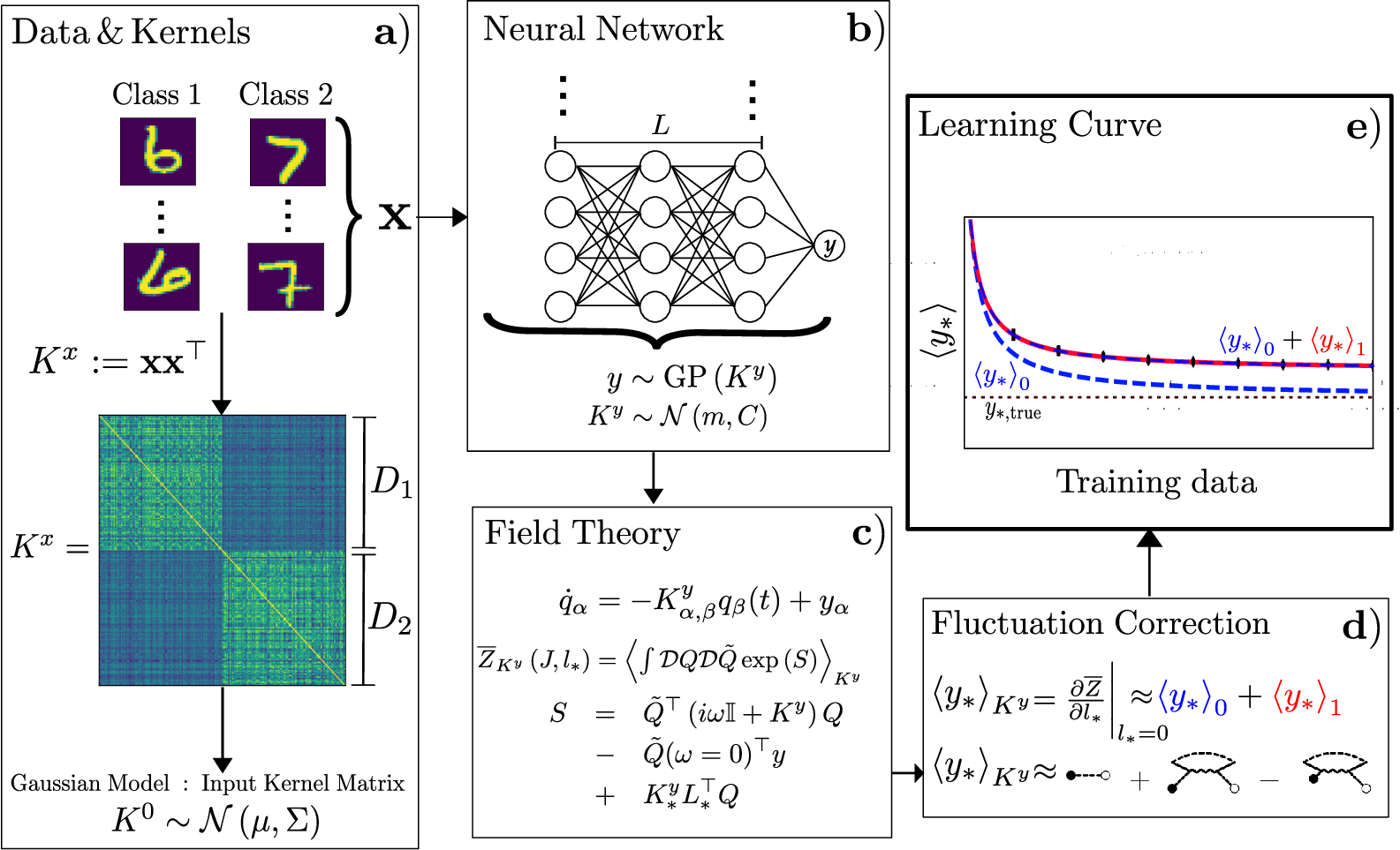
Figure 1: Field theory of generalization in Bayesian inference. a) A binary classification task, such as distinguishing pairs of digits in MNIST, can be described with the help of an overlap matrix KxK^{x} that represents similarity across the c=c1+c2c=c_{1}+c_{2} images of the training set of two classes, 11 and 22 with D1D_{1} and D2D_{2} samples respectively. Entries of the overlap matrix are heterogeneous. Different drawings of cc example patterns each lead to different realizations of the overlap matrix; the matrix is stochastic. We here describe the matrix elements by a correlated multivariate Gaussian. b) The data is fed through a feed-forward neural network to produce an output yy. In the case of infinitely wide hidden layers and under Gaussian priors on the network weights, the output of the network is a Gaussian process with the kernel KyK^{y}, which depends on the network architecture and the input kernel KxK^{x}. c) To obtain statistical properties of the posterior distribution, we compute its disorder-averaged moment generating function Z¯​(J,l∗)\overline{Z}(J,l_{*}) diagrammatically. d) The leading-order contribution from the homogeneous kernel ⟨y∗⟩0\langle y^{\ast}\rangle_{0} is corrected by ⟨y∗⟩1\langle y^{\ast}\rangle_{1} due to the variability of the overlaps; both follow as derivatives of Z¯​(J,l∗)\overline{Z}(J,l_{*}). e) Comparing the mean network output on a test point ⟨y∗⟩\left\langle y^{*}\right\rangle, the zeroth order theory ⟨y∗⟩0\left\langle y_{*}\right\rangle_{0} (blue dashed), the first-order approximation in the data-variability ⟨y∗⟩0+1\left\langle y_{*}\right\rangle_{0+1} (blue-red dashed) and empirical results (black crosses) as a function of the amount of training data (learning curve) shows how variability in the data set limits the network performance and validates the theory.

Machine learning and in particular deep learning continues to influence all areas of science . Employed as a scientific method, explainability, a defining feature of any scientific method, however, is still largely missing. This is also important to provide guarantees and to guide educated design choices to reach a desired level of accuracy. The reason is that the underlying principles by which artificial neural networks reach their unprecedented performance are largely unknown. There is, up to date, no complete theoretical framework which fully describes the behavior of artificial neural networks so that it would explain the mechanisms by which neural networks operate. Such a framework would also be useful to support architecture search and network training.

Investigating the theoretical foundations of artificial neural networks on the basis of statistical physics dates back to the 1980s. Early approaches to investigate neural information processing were mainly rooted in the spin-glass literature and included the computation of the memory capacity of the perceptron, path integral formulations of the network dynamics (Sompolinsky et al. 1988), and investigations of the energy landscape of attractor network (Amit et al. 1985; Gardner 1988; Gardner and Derrida 1988).

As in the thermodynamic limit in solid state physics, some modern approaches deal with artificial neural networks (ANN) with an infinite number of hidden neurons to simplify calculations. This leads to a relation between ANNs and Bayesian inference on Gaussian processes (Neal 1996; Williams 1996), known as the Neural Network Gaussian Process (NNGP) limit: The prior distribution of network outputs across realizations of network parameters here becomes a Gaussian process that is uniquely described by its covariance function or kernel. This approach has been used to obtain insights into the relation of network architecture and trainability (Poole et al. 2016; Schoenholz et al. 2017; Yang 2019; Cui et al. 2022; Ruben and Pehlevan 2023). Other works have investigated training by gradient descent as a means to shape the corresponding kernel (Jacot et al. 2018). A series of recent studies also captures networks at finite width, including adaptation of the kernel due to feature learning effects (Cohen et al. 2021; Naveh and Ringel 2021; Zavatone-Veth and Pehlevan 2021; Zavatone-Veth et al. 2021; Li and Sompolinsky 2021; Roberts et al. 2022; Bordelon and Pehlevan 2022). Even though training networks with gradient descent is the most abundant setup, different schemes such as Bayesian Deep Learning (Murphy 2023) provide an alternative perspective on training neural networks. Rather than finding the single-best parameter realization to solve a given task, the Bayesian approach aims to find the optimal parameter distribution.

In this work we adopt the Bayesian approach and investigate the effect of variability in the training data on the generalization properties of wide neural networks. We do so in the limit of infinitely wide linear and non-linear networks. To obtain analytical insights, we apply tools from statistical field theory to derive approximate expressions for the predictive distribution in the NNGP limit. The remainder of this work is structured in the following way: In Section II we describe the setup of supervised learning in shallow and deep networks in the framework of Bayesian inference and we introduce a synthetic data set that allows us to control the degree of pattern separability, dimensionality, and variability of the resulting overlap matrix. In Section III we develop the field theoretical approach to learning curves and its application to the synthetic data set as well as to MNIST (LeCun et al. 1998): Section III.1 presents the general formalism and shows that data variability in general leads to a non-Gaussian process. Here we also derive perturbative expressions to characterize the posterior distribution of the network output. We first illustrate these ideas on the simplest but non-trivial example of linear Bayesian regression and then generalize them first to linear and then to non-linear deep networks. In Section II.3 we show results for the synthetic data set to obtain interpretable expressions that allow us to identify how data variability affects generalization; we then illustrate the identified mechanisms on MNIST. In Section IV we summarize our findings, discuss them in the light of the literature, and provide an outlook.

II Setup

In this background section we outline the relation between neural networks, Gaussian processes, and Bayesian inference. We further present an artificial binary classification task which allows us to control the degree of pattern separation and variability and test the predictive power of the theoretical results for the network generalization properties.

II.1 Neural networks, Gaussian processes and Bayesian inference

The advent of parametric methods such as neural networks is preceded by non-parametric approaches such as Gaussian processes. There are, however, clear connections between the two concepts which allow us to borrow from the theory of Gaussian processes and Bayesian inference to describe the seemingly different neural networks. We will here give a short recap on neural networks, Bayesian inference, Gaussian processes, and their mutual relations.

II.1.1 Background: Neural Networks

In general a feed forward neural network maps inputs xα∈ℝNdimx_{\alpha}\in\mathbb{R}^{N_{\mathrm{dim}}} to outputs yα∈ℝNouty_{\alpha}\in\mathbb{R}^{N_{\mathrm{out}}} via the transformations

hα(l)\displaystyle h_{\alpha}^{(l)} =𝐖(l)ϕ(l)(hα(l−1))withhα0=𝐕xα,\displaystyle=\mathbf{W}^{(l)}\phi^{(l)}\left(h_{\alpha}^{(l-1)}\right)\quad\mathrm{with}\quad h_{\alpha}^{0}=\mathbf{V}x_{\alpha}\,,
yα\displaystyle y_{\alpha} =𝐔​ϕ(L+1)​(hα(L)),\displaystyle=\mathbf{U}\phi^{(L+1)}\left(h_{\alpha}^{(L)}\right)\,, (1)

where ϕ(l)​(x)\phi^{(l)}(x) are activation functions, 𝐕∈ℝNh×Ndim\mathbf{V\in}\,\mathbb{R}^{N_{h}\times N_{\mathrm{dim}}} are the read-in weights, NdimN_{\mathrm{dim}} is the dimension of the input, 𝐖(l)∈ℝNh×Nh\mathbf{W}^{(l)}\in\mathbb{R}^{N_{h}\times N_{h}} are the hidden weights, NhN_{h} denotes the number of hidden neurons, and 𝐔∈ℝNout×Nh\mathbf{U\in\mathbb{R}}^{N_{\mathrm{out}}\times N_{h}} are the read-out weights. Here ll is the layer index 1≤l≤L1\leq l\leq L and LL the number of layers of the network; we here assume layer- independent activation functions ϕ(l)=ϕ\phi^{(l)}=\phi. The collection of all weights are the model parameters Θ={𝐕,𝐖(1),…,𝐖(L),𝐔}\Theta=\{\mathbf{V},\mathbf{W}^{(1)},\ldots,\mathbf{W}^{(L)},\mathbf{U}\}. The goal of training a neural network in a supervised manner is to find a set of parameters Θ^\hat{\Theta} which reproduces the input-output relation (xtr,α,ytr,α)1≤α≤D\left(x_{\mathrm{tr},\alpha},y_{\mathrm{tr},\alpha}\right)_{1\leq\alpha\leq D} for a set of DD pairs of inputs and outputs as accurately as possible, while also maintaining the ability to generalize. Hence one partitions the data into a training set 𝒟tr,|𝒟tr|=D\mathcal{D}_{\mathrm{tr}}\,,\,|\mathcal{D}_{\mathrm{tr}}|=D, and a test-set 𝒟test,|𝒟test|=Dtest\mathcal{D}_{\mathrm{test}}\,,\,|\mathcal{D}_{\mathrm{test}}|=D_{\mathrm{test}}. The training data is given in the form of the matrices 𝐱tr∈ℝNdim×Ntr\mathbf{x}_{\mathrm{tr}}\in\mathbb{R}^{N_{\mathrm{dim}}\times N_{\mathrm{tr}}} and 𝐲tr∈ℝNout×Ntr\mathbf{y}_{\mathrm{tr}}\in\mathbb{R}^{N_{\mathrm{out}}\times N_{\mathrm{tr}}}. The quality of how well a neural network is able to model the relation between inputs and outputs is quantified by a task-dependent loss function ℒ⁡(Θ,xα,yα)\mathcal{L}\left(\Theta,x_{\alpha},y_{\alpha}\right). Starting with a random initialization of the parameters Θ\Theta, one tries to find an optimal set of parameters Θ^\hat{\Theta} that minimizes the loss ∑α=1Dℒ⁡(Θ,xtr,α,ytr,α)\sum_{\alpha=1}^{D}\mathcal{L}\left(\Theta,x_{\mathrm{tr},\alpha},y_{\mathrm{tr,}\alpha}\right) on the training set 𝒟tr\mathcal{D}_{\mathrm{tr}}. The parameters Θ^\hat{\Theta} are usually obtained through methods such as stochastic gradient descent. The generalization properties of the network are quantified after the training by computing the loss ℒ⁡(Θ^,xα,yα)\mathcal{L}\left(\hat{\Theta},x_{\alpha},y_{\alpha}\right) on the test set (xtest,α,ytest,α)∈𝒟test\left(x_{\mathrm{test,}\alpha},y_{\mathrm{test,}\alpha}\right)\in\mathcal{D}_{\mathrm{test}}, which are data samples that have not been used during the training process. Neural networks hence provide, by definition, a parametric modeling approach, as the goal is to a find an optimal set of parameters Θ^\hat{\Theta}.

II.1.2 Background: Bayesian inference and Gaussian processes

The parametric viewpoint in Section II.1.1 which yields a point estimate Θ^\hat{\Theta} for the optimal set of parameters can be complemented by considering a Bayesian perspective (MacKay 2003; Murphy 2022; Murphy 2023): For each network input xαx_{\alpha}, the network equations (1) yield a single output y⁡(xα|Θ)y\left(x_{\alpha}|\Theta\right). One typically considers a stochastic output y⁡(xα|Θ)+ξαy\left(x_{\alpha}|\Theta\right)+\xi_{\alpha} where the ξα\xi_{\alpha} are Gaussian independently and identically distributed (i.i.d.) with variance σreg2\sigma_{\mathrm{reg}}^{2} (Williams and Barber 1998). This regularization allows us to define the probability distribution p⁡(y|xα,Θ)=⟨δ⁡[yα−y⁡(xtr,α|Θ)−ξα]⟩ξα=𝒩⁡(yα,y⁡(xα|Θ),σreg2)p\left(y|x_{\alpha},\Theta\right)=\left\langle\delta\left[y_{\mathrm{\alpha}}-y(x_{\mathrm{tr},\alpha}|\Theta)-\xi_{\alpha}\right]\right\rangle_{\xi_{\alpha}}=\mathcal{N}\left(y_{\alpha};\,y(x_{\alpha}|\Theta),\sigma_{\mathrm{reg}}^{2}\right). An alternative interpretation of ξα\xi_{\alpha} is a Gaussian noise on the labels. Given a particular set of the network parameters Θ\Theta this implies a joint distribution p⁡(𝐲|𝐱tr,Θ):=∏α=1D⟨δ⁡[yα−y⁡(xtr,α|Θ)−ξα]⟩{ξα}=∏α=1Dp⁡(yα|xα,Θ)p\left(\mathbf{y}|\mathbf{x}_{\mathrm{tr}},\Theta\right):=\prod_{\alpha=1}^{D}\left\langle\delta\left[y_{\alpha}-y(x_{\mathrm{tr},\alpha}|\Theta)-\xi_{\alpha}\right]\right\rangle_{\{\xi_{\alpha}\}}=\prod_{\alpha=1}^{D}p(y_{\alpha}|x_{\alpha},\Theta) of network outputs {yα}1≤α≤D\{y_{\alpha}\}_{1\leq\alpha\leq D}, each corresponding to one network input {xtr,α}1≤α≤D\{x_{\mathrm{tr},\alpha}\}_{1\leq\alpha\leq D}. One aims to use the training data 𝒟tr\mathcal{D}_{\mathrm{tr}} to compute the posterior distribution for the weights 𝐕,𝐖(1),…,𝐖(L),𝐔\mathbf{V},\mathbf{W}^{(1)},\ldots,\mathbf{W}^{(L)},\mathbf{U} by conditioning on the network outputs to agree to the desired training values. Concretely, we here assume as a prior for the model parameters that the parameter elements Vi​j,Wi​j(l),Ui​jV_{ij},W_{ij}^{(l)},U_{ij} are i.i.d. according to centered Gaussian distributions Vi​j∼𝒩⁡(0,σv2/Ndim)V_{ij}\sim\mathcal{N}\left(0,\sigma_{v}^{2}/N_{\mathrm{dim}}\right), Wi​j(l)∼𝒩⁡(0,σw2/Nh)W_{ij}^{(l)}\sim\mathcal{N}\left(0,\sigma_{w}^{2}/N_{h}\right), and Ui​j∼𝒩⁡(σu2/Nh)U_{ij}\sim\mathcal{N}\left(\sigma_{u}^{2}/N_{h}\right).

The posterior distribution of the parameters p⁡(Θ|𝐱tr,𝐲tr)p\left(\Theta|\mathbf{x}_{\mathrm{tr}},\mathbf{y}_{\mathrm{tr}}\right) then follows from Bayes’ theorem as

p⁡(Θ|𝐱tr,𝐲tr)=p⁡(𝐲tr|𝐱tr,Θ)​p​(Θ)p⁡(𝐲tr|𝐱tr),p\left(\Theta|\mathbf{x}_{\mathrm{tr}},\mathbf{y}_{\mathrm{tr}}\right)=\frac{p\left(\mathbf{y}_{\mathrm{tr}}|\mathbf{x}_{\mathrm{tr}},\Theta\right)\,p\left(\Theta\right)}{p\left(\mathbf{y}_{\mathrm{tr}}|\mathbf{x}_{\mathrm{tr}}\right)}\,, (2)

with the likelihood p⁡(𝐲tr|𝐱tr,Θ)p\left(\mathbf{y}_{\mathrm{tr}}|\mathbf{x}_{\mathrm{tr}},\Theta\right), the weight prior p⁡(Θ)p\left(\Theta\right) and the model evidence p⁡(𝐲tr|𝐱tr)=∫d​Θ​p​(𝐲tr|𝐱tr,Θ)​p​(Θ)p\left(\mathbf{y}_{\mathrm{tr}}|\mathbf{x}_{\mathrm{tr}}\right)=\int d\Theta\,p\left(\mathbf{y}_{\mathrm{tr}}|\mathbf{x}_{\mathrm{tr}},\Theta\right)p\left(\Theta\right), which provides the proper normalization. The posterior parameter distribution p⁡(Θ|𝐱tr,𝐲tr)p\left(\Theta|\mathbf{x}_{\mathrm{tr}},\mathbf{y}_{\mathrm{tr}}\right) also determines the distribution of the network output y∗y_{*} corresponding to a test-point x∗x_{*} by marginalizing over the parameters Θ\Theta

p⁡(y∗|x∗,𝐱tr,𝐲tr)\displaystyle p\left(y_{*}|x_{*},\mathbf{x}_{\mathrm{tr}},\mathbf{y}_{\mathrm{tr}}\right) =∫d​Θ​p​(y∗|x∗,Θ)​p​(Θ|𝐱tr,𝐲tr),\displaystyle=\int d\Theta\,p\left(y_{*}|x_{*},\Theta\right)p\left(\Theta|\mathbf{x}_{\mathrm{tr}},\mathbf{y}_{\mathrm{tr}}\right)\,, (3)
=p(y∗,𝐲tr|x∗,𝐱tr)p⁡(𝐲tr|𝐱tr).\displaystyle=\frac{p\left(y_{*},\mathbf{y}_{\mathrm{tr}}|x_{*},\mathbf{x}_{\mathrm{tr}}\right)}{p\left(\mathbf{y}_{\mathrm{tr}}|\mathbf{x}_{\mathrm{tr}}\right)}\,. (4)

One can understand this intuitively: The distribution in (2) provides a set of viable parameters Θ\Theta based on the training data. An initial guess for the correct choice of parameters via the prior p⁡(Θ)p\left(\Theta\right) is refined, based on whether the choice of parameters accurately models the relation of the training–data, which is encapsulated in the likelihood p⁡(𝐲tr|𝐱tr,Θ)p\left(\mathbf{y}_{\mathrm{tr}}|\mathbf{x}_{\mathrm{tr}},\Theta\right). This viewpoint of Bayesian parameter selection is also equivalent to what is known as Bayesian deep learning (Murphy 2023). The distribution p(y∗,𝐲tr|x∗,𝐱tr)p\left(y_{*},\mathbf{y}_{\mathrm{tr}}|x_{*},\mathbf{x}_{\mathrm{tr}}\right) describes the joint network outputs for all training points and the test point. In the case of wide networks, where Nh→∞N_{h}\rightarrow\infty, (Neal 1996; Williams 1996) showed that the distribution of network outputs p(y∗,𝐲tr|x∗,𝐱tr)p\left(y_{*},\mathbf{y}_{\mathrm{tr}}|x_{*},\mathbf{x}_{\mathrm{tr}}\right) approaches a Gaussian process y∼𝒩⁡(0,Ky)y\sim\mathcal{N}\left(0,K^{y}\right), where the covariance ⟨yα​yβ⟩=Kα​βy\langle y_{\alpha}y_{\beta}\rangle=K_{\alpha\beta}^{y} is also denoted as the kernel. This is beneficial, as the inference for the network output y∗y_{\ast} for a test point x∗x_{\ast} then also follows a Gaussian distribution with mean and covariance given by (Rasmussen and Williams 2006)

⟨y∗⟩\displaystyle\left\langle y_{\ast}\right\rangle =K∗αy​(Ky)α​β−1​ytr,β,\displaystyle=K_{*\alpha}^{y}\left(K^{y}\right)_{\alpha\beta}^{-1}\,y_{\mathrm{tr},\beta}\,, (5)
⟨(y∗−⟨y∗⟩)2⟩\displaystyle\left\langle\left(y_{\ast}-\left\langle y_{\ast}\right\rangle\right)^{2}\right\rangle =K∗⁣∗y−K∗αy(Ky)α​β−1Kβ∗y,\displaystyle=K_{**}^{y}-K_{*\alpha}^{y}\left(\text{$K^{y}$}\right)_{\alpha\beta}^{-1}\,K_{\beta*}^{y}\,, (6)

where summation over repeated indices is implied. There has been extensive research in relating the outputs of wide neural networks to Gaussian processes (Neal 1996; Cho and Saul 2009; Lee et al. 2018) including recent work on corrections due to finite-width effects Nh≫1N_{h}\gg 1 (Cohen et al. 2021; Naveh and Ringel 2021; Zavatone-Veth and Pehlevan 2021; Zavatone-Veth et al. 2021; Li and Sompolinsky 2021; Segadlo et al. 2022; Ariosto et al. 2023; Roberts et al. 2022).

II.2 Our contribution

A fundamental assumption of supervised learning is the existence of a joint distribution p⁡(xtr,ytr)p(x_{\mathrm{tr}},y_{\mathrm{tr}}) from which the set of training data as well as the set of test data are drawn. In this work we follow the Bayesian approach and investigate the effect of variability in the training data on the generalization properties of wide neural networks. We do so in the kernel limit of infinitely wide linear and non-linear networks. Variability here has two meanings: First, for each drawing of DD pairs of training samples (xtr,α,ytr,α)1≤α≤D(x_{\mathrm{tr,}\alpha},y_{\mathrm{tr},\alpha})_{1\leq\alpha\leq D} one obtains a D×DD\times D kernel matrix KyK^{y} with heterogeneous entries; so in a single instance of Bayesian inference, the entries of the kernel matrix vary from one entry to the next. Second, each such drawing of DD training data points and one test data point (x∗,y∗)\left(x_{*},y_{*}\right) leads to a different kernel {Kα​βy}1≤α,β≤D+1\{K_{\alpha\beta}^{y}\}_{1\leq\alpha,\beta\leq D+1}, which follows some probabilistic law Ky∼p⁡(Ky)K^{y}\sim p(K^{y}).

Our work builds upon previous results for the NNGP limit to formalize the influence of such stochastic kernels. We here develop a field theoretic approach to systematically investigate the influence of the underlying kernel stochasticity on the generalization properties of the network, namely the learning curve, the dependence of ⟨y∗⟩\langle y_{\ast}\rangle on the number of training samples D=|𝒟tr|D=|\mathcal{D}_{\mathrm{tr}}|. As we assume Gaussian i.i.d. priors on the network parameters, the output kernel Kα​βyK_{\alpha\beta}^{y} solely depends on the network architecture and the input overlap matrix

Kα​βx=∑i=1Ndimxα​i​xβ​ixα,xβ∈𝒟tr∪𝒟test,K_{\alpha\beta}^{x}=\sum_{i=1}^{N_{\mathrm{dim}}}x_{\alpha i}x_{\beta i}\quad x_{\alpha},x_{\beta}\in\mathcal{D}_{\mathrm{tr}}\cup\mathcal{D}_{\mathrm{test}}\,, (7)

with α,β=1​…​D+1\alpha,\beta=1...D+1. We next define a data model which allows us to approximate the probability measure for the data variability.

II.3 Definition of a synthetic data set

To investigate the generalization properties in a binary classification task, we introduce a synthetic stochastic binary classification task. This task allows us to control the statistical properties of the data with regard to the dimensionality of the patterns, the degree of separation between patterns belonging to different classes, and the variability in the kernel. Moreover, it allows us to construct training-data sets 𝒟tr\mathcal{D}_{\mathrm{tr}} of arbitrary sizes and we will show that the statistics of the resulting kernels is indeed representative for more realistic data sets such as MNIST.

Refer to caption
Figure 2: Synthetic data set. a) Two sample vectors x(1≤α≤4)x^{(1\leq\alpha\leq 4)} for each of the two classes (upper, lower). The values for the pixels can be xi(α)∈{−1,1}x_{i}^{(\alpha)}\in\{-1,1\} where yellow indicates xi(α)=1x_{i}^{(\alpha)}=1 and blue xi(α)=−1x_{i}^{(\alpha)}=-1. The three columns correspond to three different settings of the pixel probability p∈{0.5,0.8,1}p\in\{0.5,0.8,1\}. b) Empirical overlap matrices KxK^{x} (10) for D/2=2D/2=2 patterns of class 11 and D/2=2D/2=2 patterns of class 22. The entries of the overlap matrices are Kα​βx∈[−1,1].K_{\alpha\beta}^{x}\in[-1,1]. Darker colors indicate Kα​βx≈−1K_{\alpha\beta}^{x}\approx-1 and brighter colors correspond to Kα​βx≈1K_{\alpha\beta}^{x}\approx 1. c) Empirical overlap matrix KxK^{x} for the same task as in a), b) with D=50D=50. Other parameters: Ndim=6N_{\mathrm{dim}}=6.

The data set consists of pattern realizations xα∈{−1,1}Ndimx_{\alpha}\in\{-1,1\}^{N_{\mathrm{dim}}} with dimension NdimN_{\mathrm{dim}} even. We denote the entries xα​ix_{\alpha i} of this NdimN_{\mathrm{dim}}-dimensional vector for data point α\alpha as pixels that randomly take either of two values xα​i∈{−1,1}x_{\alpha i}\in\{-1,1\} with respective probabilities p⁡(xα​i=1)p(x_{\alpha i}=1) and p⁡(xα​i=−1)p(x_{\alpha i}=-1) that depend on the class c⁡(α)∈{1,2}c(\alpha)\in\{1,2\} of the pattern realization and whether the index ii is in the left half ( i≤Ndim/2i\leq N_{\mathrm{dim}}/2) or the right half ( i>Ndim/2i>N_{\mathrm{dim}}/2) of the pattern: For class c⁡(α)=1c(\alpha)=1 each pixel xα​i​with​ 1≤i≤Ndimx_{\alpha i}\,\mathrm{with\,}1\leq i\leq N_{\mathrm{dim}} is realized independently as a binary variable as

xα​i\displaystyle x_{\alpha i} ={1with​p−1with⁡(1−p)for​i≤Ndim2,\displaystyle=\begin{cases}1&\mathrm{with}\,\>p\\ -1&\mathrm{with}\,\>(1-p)\end{cases}\quad\mathrm{for}\,\,i\leq\frac{N_{\mathrm{dim}}}{2}\,, (8)
xα​i\displaystyle x_{\alpha i} ={1with⁡(1−p)−1with​pfor​i>Ndim2.\displaystyle=\begin{cases}1&\mathrm{with}\,\>(1-p)\\ -1&\mathrm{with}\,\>p\end{cases}\quad\mathrm{for}\,\,i>\frac{N_{\mathrm{dim}}}{2}\,. (9)

For a pattern xαx_{\alpha} in the second class c⁡(α)=2c(\alpha)=2 the pixel values are distributed independently of those in the first class with a statistics that equals the negative pixel values of the first class, which is P⁡(xα​i)=P⁡(−xβ​i)P\left(x_{\alpha i}\right)=P\left(-x_{\beta i}\right) with c⁡(β)=1c(\beta)=1 and c⁡(α)=2c(\alpha)=2. There are two limiting cases for pp which illustrate the construction of the patterns: In the limit p=1p=1, each pattern xαx_{\alpha} in c=1c=1 consists of a vector, where the first Ndim/2N_{\mathrm{dim}}/2 pixels have the value xα​i=1x_{\alpha i}=1, whereas the second half consists of pixels with the value xα,i=−1x_{\alpha,i}=-1. The opposite holds for patterns in the second class c=2c=2. This limiting case is shown in Figure 2 (right column). In the limit case p=0.5p=0.5 each pixel assumes the value xα,i=±1x_{\alpha,i}=\pm 1 with equal probability, regardless of the pattern class-membership or the pixel position. Hence one cannot distinguish the class membership of any of the training instances. This limiting case is shown in Figure 2 (left column). If c⁡(α)=1c(\alpha)=1 we set ytr,α=−1y_{\mathrm{tr},\alpha}=-1 and for c⁡(α)=2c(\alpha)=2 we set ytr,α=1y_{\mathrm{tr},\alpha}=1.We now investigate the description of this task in the framework of Bayesian inference. The hidden variables hα0h_{\alpha}^{0} (1) in the input layer under a Gaussian prior on Vi​j∼𝒩⁡(0,σv2/Ndim)V_{ij}\mathrel{{\mathop{\sim}\limits}}\mathcal{N}\left(0,\sigma_{v}^{2}/N_{\mathrm{dim}}\right) follow a Gaussian process with kernel K(0)K^{(0)} given by

Kα​β0\displaystyle K_{\alpha\beta}^{0} =⟨hα0​hβ0⟩V∼𝒩⁡(0,σv2Ndim),\displaystyle=\langle h_{\alpha}^{0}h_{\beta}^{0}\rangle_{V\sim\mathcal{N}\left(0,\frac{\sigma_{v}^{2}}{N_{\mathrm{dim}}}\right)}\,, (10)
=σv2Ndim​∑i=1Ndimxα​i​xβ​i.\displaystyle=\frac{\sigma_{v}^{2}}{N_{\mathrm{dim}}}\,\sum_{i=1}^{N_{\mathrm{dim}}}x_{\alpha i}x_{\beta i}\,. (11)

Separability of the two classes is reflected in the structure of this input kernel K0K^{0} as shown in Figure 2: In the cases with p=0.8p=0.8 and p=1p=1 one can clearly distinguish blocks; the diagonal blocks represent intra-class overlaps, the off-diagonal blocks inter-class overlaps. This is not the case for p=0.5p=0.5, where no clear block-structure is visible. In the case of p=0.8p=0.8 one can further observe that the blocks are not as clear-cut as in the case p=1p=1, but rather noisy, similar to p=0.5p=0.5. This is due to the probabilistic realization of patterns, which induces stochasticity in the blocks of the input kernel K0K^{0} (10). To quantify this effect, based on the distribution of the pixel values (9) we compute the distribution of the entries of K0K^{0} for the binary classification task. The mean of the overlap elements μα​β\mu_{\alpha\beta} and their covariances Σ(α​β)​(γ​δ)\Sigma_{(\alpha\beta)(\gamma\delta)} are defined via

μα​β\displaystyle\mu_{\alpha\beta} =⟨Kα​β0⟩,\displaystyle=\left\langle K_{\alpha\beta}^{0}\right\rangle\,, (12)
Σ(α​β)​(γ​δ)\displaystyle\Sigma_{(\alpha\beta)(\gamma\delta)} =⟨δ​Kα​β0​δ​Kγ​δ0⟩,\displaystyle=\left\langle\delta K_{\alpha\beta}^{0}\,\delta K_{\gamma\delta}^{0}\right\rangle\,, (13)
δ​Kα​β0\displaystyle\delta K_{\alpha\beta}^{0} =Kα​β0−μα​β,\displaystyle=K_{\alpha\beta}^{0}-\mu_{\alpha\beta}\,, (14)

where the expectation value ⟨⋅⟩\left\langle\cdot\right\rangle is taken over drawings of DD training samples each. By construction we have μα​β=μβ​α\mu_{\alpha\beta}=\mu_{\beta\alpha}. The covariance is further invariant under the exchange of (α,β)↔(γ,δ)(\alpha,\beta)\leftrightarrow(\gamma,\delta) and, due to the symmetry of Kα​β0=Kβ​α0K_{\alpha\beta}^{0}=K_{\beta\alpha}^{0}, also under swapping α↔β\alpha\leftrightarrow\beta and γ↔δ\gamma\leftrightarrow\delta separately. In the artificial task-setting, the parameter pp, the pattern dimensionality NdimN_{\mathrm{dim}}, and the variance σv2/Ndim\sigma_{v}^{2}/N_{\mathrm{dim}} of each read-in weight Vi​jV_{ij} define the elements of μα​β\mu_{\alpha\beta} and Σ(α​β)​(γ​δ)\Sigma_{(\alpha\beta)(\gamma\delta)}, which read (see Supplement .1)

μα​β\displaystyle\mu_{\alpha\beta} =σv2​{1α=βucα=cβ−ucα≠cβ,\displaystyle=\sigma_{v}^{2}\,\begin{cases}1&\alpha=\beta\\ u&c_{\alpha}=c_{\beta}\\ -u&c_{\alpha}\neq c_{\beta}\end{cases}\,,
Σ(α​β)​(α​β)\displaystyle\Sigma_{(\alpha\beta)(\alpha\beta)} =σv4Ndim​κ,\displaystyle=\frac{\sigma_{v}^{4}}{N_{\mathrm{dim}}}\kappa,
Σ(α​β)​(α​δ)\displaystyle\Sigma_{(\alpha\beta)(\alpha\delta)} =σv4Ndim​{νfor​{cα=cβ=cδcα≠cβ=cδ−νfor​{cα=cβ≠cδcα=cδ≠cβ,\displaystyle=\frac{\sigma_{v}^{4}}{N_{\mathrm{dim}}}\begin{cases}\nu&\mathrm{for}\,\begin{cases}c_{\alpha}=c_{\text{$\beta$}}=c_{\text{$\delta$}}\\ c_{\alpha}\neq c_{\beta}=c_{\delta}\end{cases}\\ -\nu&\mathrm{for}\,\begin{cases}c_{\alpha}=c_{\beta}\neq c_{\delta}\\ c_{\alpha}=c_{\delta}\neq c_{\beta}\end{cases}\end{cases}\,,
withκ\displaystyle\mathrm{with\quad}\kappa :=1−u2,\displaystyle:=1-u^{2}\,,
ν\displaystyle\nu :=u⁡(1−u),\displaystyle:=u\,(1-u)\,,
u\displaystyle u :=4​p​(p−1)+1.\displaystyle:=4p(p-1)+1\,. (15)

In addition to this, the tensor elements of Σ(α​β)​(γ​δ)\Sigma_{(\alpha\beta)(\gamma\delta)} are zero for the following index combinations because we fixed the value of Kα​α0K_{\alpha\alpha}^{0} by construction:

Σ(α​β)​(γ​δ)\displaystyle\Sigma_{(\alpha\beta)(\gamma\delta)} =0withα≠β≠γ≠δ,\displaystyle=0\quad\mathrm{with\quad\alpha\neq\beta\neq\gamma\neq\delta}\,,
Σ(α​α)​(β​γ)\displaystyle\Sigma_{(\alpha\alpha)(\beta\gamma)} =0withα≠β≠γ,\displaystyle=0\quad\text{with$\quad\alpha\neq\beta\neq\gamma$}\,,
Σ(α​α)​(β​β)\displaystyle\Sigma_{(\alpha\alpha)(\beta\beta)} =0withα≠β,\displaystyle=0\quad\mathrm{with\quad\alpha\neq\beta}\,,
Σ(α​α)​(α​β)\displaystyle\Sigma_{(\alpha\alpha)(\alpha\beta)} =0withα≠β,\displaystyle=0\quad\mathrm{with\quad\alpha\neq\beta}\,,
Σ(α​α)​(α​α)\displaystyle\Sigma_{(\alpha\alpha)(\alpha\alpha)} =0withα≠β.\displaystyle=0\quad\mathrm{with\quad\alpha\neq\beta}\,. (16)

The expressions for Σ(α​β)​(α​β)\Sigma_{(\alpha\beta)(\alpha\beta)} and Σ(α​β)​(α​δ)\Sigma_{(\alpha\beta)(\alpha\delta)} in (15) show that the magnitude of the fluctuations are controlled through the parameter pp and the pattern dimensionality NdimN_{\mathrm{dim}}: The covariance Σ\Sigma is suppressed by a factor of 1/Ndim1/N_{\mathrm{dim}} compared to the mean values μ\mu. Hence we can use the pattern dimensionality NdimN_{\mathrm{dim}} to investigate the influence of the strength of fluctuations. As illustrated in Figure 1a, the elements Σ(α​β)​(α​β)\Sigma_{(\alpha\beta)(\alpha\beta)} denote the variance of individual entries of the kernel, while Σ(α​β)​(α​γ)\Sigma_{(\alpha\beta)(\alpha\gamma)} are covariances of entries across elements of a given row α\alpha, visible as horizontal or vertical stripes in the color plot of the kernel.

Equation (15) implies, by construction, a Gaussian distribution of the elements Kα​β0K_{\alpha\beta}^{0} as it only provides the first two cumulants. One can show that the higher-order cumulants of Kα​β0K_{\alpha\beta}^{0} scale sub-leading in the pattern dimension and are hence suppressed by a factor 𝒪⁡(1/Ndim)\mathcal{O}\left(1/N_{\mathrm{dim}}\right) compared to Σ(α​β)​(γ​δ)\Sigma_{(\alpha\beta)(\gamma\delta)}.

III Results

In this section we derive the field theoretic formalism which allows us to compute the statistical properties of the inferred network output in Bayesian inference with a stochastic kernel. We show that the resulting process is non-Gaussian and reminiscent of a φ3+φ4\varphi^{3}+\varphi^{4}-theory. Specifically, we compute the mean of the predictive distribution of this process conditioned on the training data. This is achieved by employing systematic approximations with the help of Feynman diagrams.

Subsequently we show that our results provide an accurate bound on the generalization capabilities of the network. We further discuss the implications of our analytic results for neural architecture search.

III.1 Field theoretic description of Bayesian inference

III.1.1 Bayesian inference with stochastic kernels

In general, a network implements a map from the inputs xαx_{\alpha} to corresponding outputs yαy_{\alpha}. In particular a model of the form (1) implements a non-linear map ψ:ℝNdim→ℝNh\psi:\mathbb{R}^{N_{\mathrm{dim}}}\rightarrow\mathbb{R}^{N_{h}} of the input xα∈ℝNdimx_{\alpha}\in\mathbb{R}^{N_{\mathrm{dim}}} to a hidden state hα∈ℝNhh_{\alpha}\in\mathbb{R}^{N_{h}}. This map may also involve multiple hidden-layers, biases and non-linear transformations. The read-out weight 𝐔∈ℝ1×Nh\mathbf{U}\in\mathbb{R}^{1\times N_{h}} links the scalar network output yα∈ℝy_{\alpha}\in\mathbb{R} and the transformed inputs ψ⁡(xα)\psi\left(x_{\alpha}\right) with 1≤α≤Dtot=D+Dtest1\leq\alpha\leq D_{\mathrm{tot}}=D+D_{\mathrm{test}} which yields

yα=𝐔​ψ​(xα)+ξα,y_{\alpha}=\mathbf{U}\,\psi\left(x_{\alpha}\right)+\xi_{\alpha}\,, (17)

where ξα∼𝒩⁡(0,σreg2)\xi_{\alpha}\mathrel{{\mathop{\sim}\limits}}\mathcal{N}(0,\sigma_{\mathrm{reg}}^{2}) is a regularization noise in the same spirit as in (Williams and Barber 1998). We assume that the prior on the read-out vector elements is a Gaussian 𝐔i​∼𝒩⁡(0,σu2/Nh). \mathbf{U}_{i}\text{$\mathrel{{\mathop{\sim}\limits}}\mathcal{N}\left(0,\sigma_{u}^{2}/N_{h}\right)$. }The distribution of the set of network outputs y1≤α≤Dtoty_{1\leq\alpha\leq D_{\mathrm{tot}}} is then in the limit Nh→∞N_{h}\rightarrow\infty a multivariate Gaussian (Neal 1996). The kernel matrix of this Gaussian is obtained by taking the expectation value with respect to the read-out vector, which yields

⟨yα​yβ⟩𝐔\displaystyle\left\langle y_{\alpha}\,y_{\beta}\right\rangle_{\mathbf{U}} =:Kα​βy=σu2​Kα​βψ+δα​β​σreg2,\displaystyle=:K_{\alpha\beta}^{y}=\sigma_{u}^{2}\,K_{\alpha\beta}^{\psi}+\delta_{\alpha\beta}\,\sigma_{\mathrm{reg}}^{2}\,, (18)
Kα​βψ\displaystyle K_{\alpha\beta}^{\psi} =1Nh​∑i=1Nhψi​(xα)​ψi​(xβ).\displaystyle=\frac{1}{N_{h}}\,\sum_{i=1}^{N_{h}}\psi_{i}\left(x_{\alpha}\right)\,\psi_{i}\left(x_{\beta}\right)\,. (19)

The kernel matrix Kα​βyK_{\alpha\beta}^{y} describes the covariance of the network’s output and hence depends on the kernel matrix Kα​βψK_{\alpha\beta}^{\psi}. The additional term δα​β​σreg2\delta_{\alpha\beta}\,\sigma_{\mathrm{reg}}^{2} acts as a regularization term, which is also known as a ridge regression (Hoerl and Kennard 2000) or Tikhonov regularization (Williams and Rasmussen 2006). In the context of neural networks one can motivate the regularizer σreg2\sigma_{\mathrm{reg}}^{2} by using the L2L^{2}-regularization in the readout layer. This is also known as weight decay (Goodfellow et al. 2016). Introducing the regularizer σreg2\sigma_{\mathrm{reg}}^{2} is necessary to ensure that one can properly invert the matrix Kα​βyK_{\alpha\beta}^{y}, ensuring that the expressions (5) and (6) are numerically stable.

Different drawings of sets of training data 𝒟tr\mathcal{D}_{\mathrm{tr}} lead to different realizations of kernel matrices KψK^{\psi} and KyK^{y}. The network output yαy_{\alpha} hence follows a multivariate Gaussian with a stochastic kernel matrix KyK^{y}. A more formal derivation of the Gaussian statistics, including an argument for its validity in deep neural networks, can be found in (Lee et al. 2018). A consistent derivation using field theoretical methods and corrections in terms for the width of the hidden layer NhN_{h} for deep and recurrent networks has been presented in (Segadlo et al. 2022).

In general, the input kernel matrix K0K^{0} (10) and the output kernel matrix KyK^{y} are related in a non-trivial fashion, which depends on the specific network architecture at hand. From now on we make an assumption on the stochasticity of K0K^{0} and assume that the input kernel matrix K0K^{0} is distributed according to a multivariate Gaussian

K0\displaystyle K^{0} ∼𝒩⁡(μ,Σ),\displaystyle\sim\mathcal{N}\left(\mu,\>\Sigma\right)\,, (20)

where μ\mu and Σ\Sigma are given by (12) and (13), respectively.

In the limit of large pattern dimensions Ndim≫N_{\mathrm{dim}}\gg1 this assumption is warranted for the kernel matrix K0K^{0}. This structure further assumes, that the overlap statistics are unimodal, which is indeed mostly the case for data such as MNIST (see Appendix .4). Furthermore we assume that this property holds for the output kernel matrix KyK^{y} as well and that we can find a mapping from the mean μ\mu and covariance Σ\Sigma of the input kernel to the mean mm and covariance CC of the output kernel (μα​β,Σ(α​β)​(γ​δ))→(mα​β,C(α​β)​(γ​δ))\left(\mu_{\alpha\beta},\>\Sigma_{(\alpha\beta)(\gamma\delta)}\right)\rightarrow\left(m_{\alpha\beta},\>C_{(\alpha\beta)(\gamma\delta)}\right) so that KyK^{y} is also distributed according to a multivariate Gaussian

Ky\displaystyle K^{y} ∼𝒩⁡(m,C).\displaystyle\sim\mathcal{N}(m,\>C)\,. (21)

For each realization Kα​βyK_{\alpha\beta}^{y}, the joint distribution of the network outputs y1≤α≤Dtoty_{1\leq\alpha\leq D_{\mathrm{tot}}} corresponding to the training and test data points 𝐱\mathbf{x} follow a multivariate Gaussian

p⁡(𝐲|𝐱)∼𝒩⁡(0,Ky).p\left(\mathbf{y}|\mathbf{x}\right)\sim\mathcal{N}\big(0,K^{y}\big)\,. (22)

The kernel allows us to compute the conditional probability p⁡(y∗|𝐱tr,𝐲tr,x∗)p\left(y_{\ast}|\mathbf{x}_{\mathrm{tr}},\mathbf{y}_{\mathrm{tr}},x_{\ast}\right), as defined in (3), for a test point (x∗,y∗)∈𝒟test(x_{\ast},y_{\ast})\in\mathcal{D}_{\mathrm{test}} conditioned on the data from the training set (𝐱tr,𝐲tr)∈𝒟tr(\mathbf{x}_{\mathrm{tr}},\mathbf{y}_{\mathrm{tr}})\in\mathcal{D}_{\mathrm{tr}}. This distribution is Gaussian with mean and variance given by (5) and (6), respectively. It is our goal to take into account that K0K^{0} is a stochastic quantity, which depends on the particular draw of the training and test data set (𝐱tr,𝐲tr)∈𝒟tr,(x∗,y∗)∈𝒟test(\mathbf{x}_{\mathrm{tr}},\mathbf{y}_{\mathrm{tr}})\in\mathcal{D}_{\mathrm{tr}},(x_{\ast},y_{\ast})\in\mathcal{D}_{\mathrm{test}}. The labels 𝐲tr,y∗\mathbf{y}_{\mathrm{tr}},y_{*} are, by construction, deterministic and take either one of the values ±1\pm 1. In the following we investigate the dependence of the mean of the predictive distribution on the number of training samples, which we call the learning curve. A common assumption is that this learning curve is rather insensitive to the very realization of the chosen training points. Thus we assume that the learning curve is self-averaging. The mean computed for a single draw of the training data is hence expected to agree well to the average over many such drawings. Under this assumption it is sufficient to compute the data-averaged mean inferred network output, which reduces to computing the disorder-average of the following quantity

⟨y∗⟩Ky\displaystyle\left\langle y_{*}\right\rangle_{K^{y}} =⟨K∗αy​[Ky]α​β−1⟩Ky​yβ.\displaystyle=\left\langle K_{*\alpha}^{y}\left[K^{y}\right]_{\alpha\beta}^{-1}\right\rangle_{K^{y}}y_{\beta}\,. (23)

To perform the disorder average and to compute perturbative corrections, we will follow these steps

  • •

    construct a suitable dynamic moment-generating function Z⁡(Ky)Z(K^{y}) ,

  • •

    propagate the input stochasticity to the network output Kα​β0→Kα​βyK_{\alpha\beta}^{0}\rightarrow K_{\alpha\beta}^{y},

  • •

    disorder-average the functional using the model Kα​βy∼𝒩⁡(mα​β,C(α​β)​(γ​δ))K_{\alpha\beta}^{y}\sim\mathcal{N}(m_{\alpha\beta},\>C_{(\alpha\beta)(\gamma\delta)}),

  • •

    and finally perform the computation of perturbative corrections using diagrammatic techniques.

III.1.2 Constructing the dynamic moment generating function

Our ultimate goal is to compute learning curves. Therefore we want to evaluate the disorder averaged mean inferred network output (23). Both the presence of two correlated random matrices and the fact that one of the matrices appears as an inverse complicate this process. One alternative route is to define the moment-generating function

Z⁡(l∗)\displaystyle Z(l_{*}) =∫d​y∗​exp⁡(l∗​y∗)​p​(y∗|x∗,𝐱tr,𝐲tr),\displaystyle=\int dy_{*}\exp(l_{*}y_{*})p\left(y_{*}|x_{*},\mathbf{x}_{\mathrm{tr}},\mathbf{y}_{\mathrm{tr}}\right)\,, (24)
=∫dy∗exp(l∗y∗)p(y∗,𝐲tr|x∗,𝐱tr)p⁡(𝐲tr|𝐱tr),\displaystyle=\frac{\int dy_{*}\exp(l_{*}y_{*})p\left(y_{*},\mathbf{y}_{\mathrm{tr}}|x_{*},\mathbf{x}_{\mathrm{tr}}\right)}{p\left(\mathbf{y}_{\mathrm{tr}}|\mathbf{x}_{\mathrm{tr}}\right)}\,, (25)
=:𝒵⁡(l∗)𝒵⁡(0),\displaystyle=:\frac{\mathcal{Z}(l_{*})}{\mathcal{Z}(0)}\,, (26)

with joint Gaussian distributions p(y∗,𝐲tr|x∗,𝐱tr)p\left(y_{*},\mathbf{y}_{\mathrm{tr}}|x_{*},\mathbf{x}_{\mathrm{tr}}\right) and p⁡(𝐲tr|𝐱tr)p\left(\mathbf{y}_{\mathrm{tr}}|\mathbf{x}_{\mathrm{tr}}\right) that each can be readily averaged over KyK^{y}. Equation (23) is then obtained as

⟨y∗⟩Ky=∂∂l∗⟨𝒵⁡(l∗)𝒵⁡(0)⟩Ky|l∗=0.\left\langle y_{*}\right\rangle_{K^{y}}=\frac{\partial}{\partial l_{*}}\left\langle\frac{\mathcal{Z}(l_{*})}{\mathcal{Z}(0)}\right\rangle_{K^{y}}\bigg\rvert_{l_{*}=0}\,. (27)

A complication of this approach is that the numerator and denominator co-fluctuate. The common route around this problem is to consider the cumulant-generating function W⁡(l∗)=ln⁡𝒵⁡(l∗)W(l_{*})=\ln\mathcal{\mathcal{Z}}(l_{*}) and to obtain ⟨y∗⟩Ky=∂∂l∗​⟨W⁡(l∗)⟩Ky\left\langle y_{*}\right\rangle_{K^{y}}=\frac{\partial}{\partial l_{*}}\left\langle W(l_{\ast})\right\rangle_{K^{y}}, which, however, requires averaging the logarithm. This is commonly done with the replica trick (Fischer and Hertz 1991; Mezard and Montanari 2009).

We here follow a different route to ensure that the disorder-dependent normalization 𝒵⁡(0)\mathcal{Z}(0) drops out and construct a dynamic moment generating function (De Dominicis 1978). Our goal is hence to design a dynamic process where a time dependent observable is related to y∗y_{*}, our mean-inferred network output. We hence define the linear process in the auxiliary variables qαq_{\alpha}

∂qα​(t)∂t\displaystyle\frac{\partial q_{\alpha}(t)}{\partial t} =−Kα​βy​qβ​(t)+yα,\displaystyle=-K_{\alpha\beta}^{y}\,q_{\beta}(t)+y_{\alpha}\,, (28)

for (xα,yα)∈𝒟tr(x_{\alpha},y_{\alpha})\in\mathcal{D}_{\mathrm{tr}}. From this we see directly that qα​(t→∞)=[Ky]α​β−1​yβq_{\alpha}(t\rightarrow\infty)=\left[K^{y}\right]_{\alpha\beta}^{-1}\,y_{\beta} is a fixpoint. The fact that Kα​βyK_{\alpha\beta}^{y} is a covariance matrix ensures that it is positive semi-definite and hence implies the convergence to a fixpoint. We can obtain (5) ⟨y∗⟩=K∗αy​[Ky]α​β−1​yβ\left\langle y_{*}\right\rangle=K_{*\alpha}^{y}\left[K^{y}\right]_{\alpha\beta}^{-1}\,y_{\beta} from (28) as a linear readout of qα​(t→∞)q_{\alpha}(t\rightarrow\infty) with the matrix K∗αyK_{*\alpha}^{y}. Using the Martin-Siggia-Rose-deDominicis-Janssen (MSRDJ) formalism (Martin et al. 1973; Janssen 1976; Stapmanns et al. 2020; Helias and Dahmen 2020) one can express this as the first functional derivative of the moment generating function Z⁡(L∗,Ky)Z(L_{*},K^{y}) in frequency space

Z⁡(L∗,Ky)\displaystyle Z(L_{*},K^{y}) =∫𝒟⁡{Q,Q~}​exp⁡(S⁡(Q,Q~,L∗)),\displaystyle=\int\mathcal{D}\{Q,\tilde{Q}\}\exp\left(S(Q,\tilde{Q},L_{*})\right)\,, (29)
S⁡(Q,Q~,L∗)\displaystyle S(Q,\tilde{Q},L_{*}) =Q~α⊤​(i​ω​𝕀+Ky)α​β​Qβ\displaystyle=\tilde{Q}_{\alpha}^{\top}\left(i\omega\mathbb{I}+K^{y}\right)_{\alpha\beta}Q_{\beta} (30)
−Q~α0​yα\displaystyle-\tilde{Q}_{\alpha}^{0}y_{\alpha}
+K∗αy​L∗⊤​Qα,\displaystyle+K_{*\alpha}^{y}L_{*}^{\top}Q_{\alpha}\,, (31)

where Q~α⊤​(⋯)​Qβ=12​π​∫d​ω​Q~α​(−ω)​(⋯)​Qβ​(OPENω)CLOSE\tilde{Q}_{\alpha}^{\top}\,(\cdots)\,Q_{\beta}=\frac{1}{2\pi}\int d\omega\tilde{Q}_{\alpha}(-\omega)\,(\cdots)\,Q_{\beta}(\text{$\omega)$} and Q~α​(ω=0)=Q~α0\tilde{Q}_{\alpha}(\omega=0)=\tilde{Q}_{\alpha}^{0}. As Z⁡(L∗,Ky)Z(L_{*},K^{y}) is normalized such that Z⁡(0,Ky)=1∀KyZ(0,K^{y})=1\quad\forall\,K^{y}, we can compute (23) by evaluating the functional derivative of the disorder-averaged moment-generating function Z¯​(L∗)\overline{Z}(L_{*}) (see Appendix .1) at t→∞t\rightarrow\infty:

Z¯​(L∗)\displaystyle\overline{Z}\left(L_{*}\right) =⟨∫𝒟⁡{Q,Q~}​exp⁡(S⁡(Q,Q~,L∗))⟩Ky,\displaystyle=\left\langle\int\mathcal{D}\{Q,\tilde{Q}\}\exp\left(S(Q,\tilde{Q},L_{*})\right)\right\rangle_{K^{y}}\,, (32)
⟨y∗⟩Ky\displaystyle\left\langle y_{*}\right\rangle_{K^{y}} =limt→∞∫dωexp(iωt)δ​Z¯​(L∗)δ​L∗​(−ω)|L∗​(−ω)=0.\displaystyle=\lim_{t\rightarrow\infty}\int d\omega\exp(i\omega t)\frac{\delta\overline{Z}\left(L_{*}\right)}{\delta L_{*}(-\omega)}\bigg\rvert_{L_{*}(-\omega)=0}\,. (33)

By construction the distribution of the kernel matrix entries Kα​βyK_{\alpha\beta}^{y} is a multivariate Gaussian (20). In the following we will treat the stochasticity of Kα​βyK_{\alpha\beta}^{y} perturbatively to gain insights into the influence of input stochasticity.

III.1.3 Perturbative treatment of the disorder averaged moment generating function

To compute the disorder averaged mean-inferred network output (23) we need to compute the disorder average of the dynamic moment generating function Z¯​(L∗)=⟨Z⁡(L∗,Ky)⟩Ky\overline{Z}(L_{*})=\left\langle Z(L_{*},K^{y})\right\rangle_{K^{y}} and its functional derivative at L∗​(ω)=0L_{*}(\omega)=0. Due to the linear appearance of KyK^{y} in the action (30) and the Gaussian distribution for KyK^{y} (21) we perform the disorder average directly and obtain the action

Z¯​(L∗)\displaystyle\overline{Z}\left(L_{*}\right) =⟨Z⁡(L∗,Ky)⟩Ky\displaystyle=\left\langle Z(L_{*},K^{y})\right\rangle_{K^{y}} (34)
:=∫𝒟⁡{Q,Q~}​exp⁡(S¯​(Q,Q~,L∗)),\displaystyle:=\int\mathcal{D}\{Q,\tilde{Q}\}\exp\left(\overline{S}(Q,\tilde{Q},L_{*})\right)\,, (35)
S¯​(Q,Q~,L∗)\displaystyle\overline{S}(Q,\tilde{Q},L_{*}) =Q~α⊤​[i​ω​𝕀α​β+mα​β]​Qβ\displaystyle=\tilde{Q}_{\alpha}^{\top}\left[i\omega\mathbb{I}_{\alpha\beta}+m_{\alpha\beta}\right]Q_{\beta} (36)
−Q~α0​yα\displaystyle-\tilde{Q}_{\alpha}^{0}y_{\alpha}
+m∗α​L∗⊤​Qα\displaystyle+m_{*\alpha}L_{*}^{\top}Q_{\alpha}
+12​C(α​β)​(γ​δ)​Q~α⊤​Qβ​Q~γ⊤​Qδ\displaystyle+\frac{1}{2}C_{(\alpha\beta)(\gamma\delta)}\tilde{Q}_{\alpha}^{\top}Q_{\beta}\tilde{Q}_{\gamma}^{\top}Q_{\delta}
+C(∗α)(βγ)L∗⊤QαQ~β⊤Qγ+𝒪(L∗2),\displaystyle+C_{(*\alpha)(\beta\gamma)}L_{*}^{\top}Q_{\alpha}\tilde{Q}_{\beta}^{\top}Q_{\gamma}+\mathcal{O}\left(L_{*}^{2}\right)\,, (37)

with Q~0:=Q~​(ω=0)\tilde{Q}^{0}:=\tilde{Q}(\omega=0) (for details see Appendix .1). As we ultimately aim to obtain corrections for the mean inferred network output ⟨y∗⟩Ky\left\langle y_{\ast}\right\rangle_{K^{y}}, we utilize the action in (37) and established results from field theory to derive the leading order terms as well as perturbative corrections diagrammatically. The presence of the variance and covariance terms in (37) introduces corrective factors, which cannot appear in the zeroth-order approximation, which corresponds to the homogeneous kernel that neglects fluctuations in KyK^{y} by setting C(α​β)​(γ​δ)=0C_{(\alpha\beta)(\gamma\delta)}=0. This will provide us with the tools to derive an asymptotic bound for the mean inferred network output ⟨y∗⟩\left\langle y^{*}\right\rangle in the case of an infinitely large training data set. This bound is directly controlled by the variability in the data. We provide empirical evidence for our theoretical results for linear, non-linear, and deep-kernel-settings and show how the results could serve as indications to aid neural architecture search based on the statistical properties of the underlying data set.

III.1.4 Field theoretic elements to compute the mean inferred network output ⟨y∗⟩Ky\left\langle y_{\ast}\right\rangle_{K^{y}}

The field theoretic description of the inference problem in form of an action (37) allows us to derive perturbative expressions for the statistics of the inferred network output ⟨y∗⟩Ky\left\langle y_{*}\right\rangle_{K^{y}} in a diagrammatic manner. This diagrammatic treatment for perturbative calculations is a powerful tool and is standard practice in statistical physics (Zinn-Justin 1996), data analysis and signal reconstruction (Ensslin and Frommert 2010), and more recently in the investigation of artificial neural networks (Dyer and Gur-Ari 2019; Fischer et al. 2022).

Comparing the action (37) to prototypical expressions from classical statistical field theory such as the φ3+φ4\varphi^{3}+\varphi^{4} theory(Zinn-Justin 1996; Helias and Dahmen 2020) one can similarly associate the elements of a field theory:

  • •

    −Q~α0​yα≐-\tilde{Q}_{\alpha}^{0}y_{\alpha}\doteq††feynman-diagram: (Feynman diagram, (x1)is a monopole term

  • •

    m∗α​L∗⊤​Qα≐m_{*\alpha}L_{*}^{\top}Q_{\alpha}\doteq ††feynman-diagram: (Feynman diagram, (x1)is a source term

  • •

    Δα​β:=(−i​ω​𝕀−m)α​β−1≐\Delta_{\alpha\beta}:=\left(-i\omega\mathbb{I}-m\right)_{\alpha\beta}^{-1}\doteq ††feynman-diagram: (Feynman diagram, (x2) is a propagator that connect the fields Qα​(ω),Q~β​(−ω)Q_{\alpha}(\omega),\tilde{Q}_{\beta}\left(-\omega\right)

  • •

    C(∗α)(βγ)L∗⊤QαQ~β⊤Qγ≐C_{(*\alpha)(\beta\gamma)}L_{*}^{\top}Q_{\alpha}\tilde{Q}_{\beta}^{\top}Q_{\gamma}\doteq††feynman-diagram: (Feynman diagram, (x3)is a three-point vertex

  • •

    12​C(α​β)​(γ​δ)​Q~α⊤​Qβ​Q~γ⊤​Qδ≐\frac{1}{2}C_{(\alpha\beta)(\gamma\delta)}\tilde{Q}_{\alpha}^{\top}Q_{\beta}\tilde{Q}_{\gamma}^{\top}Q_{\delta}\doteq††feynman-diagram: (Feynman diagram, (x3) is a four-point vertex.

The following rules for Feynman diagrams simplify calculations:

  1. 1.

    To obtain corrections to first order in C∼𝒪⁡(1/Ndim)C\sim\mathcal{O}\left(1/N_{\mathrm{dim}}\right), one has to compute all diagrams with a single vertex (three-point or four-point) (Helias and Dahmen 2020). This approach assumes that the interaction terms C(α​β)​(γ​δ)C_{(\alpha\beta)(\gamma\delta)} that stem from the variability of the data are small compared to the mean mα​βm_{\alpha\beta}. In the case of strong heterogeneity one cannot use a conventional expansion in the number of vertices C(α​β)​(γ​δ)C_{(\alpha\beta)(\gamma\delta)} and would have to resort to other methods.

  2. 2.

    Vertices, source terms, and monopoles have to be connected with one another using the propagator Δα​β=(−i​ω​𝕀−m)α​β−1\Delta_{\alpha\beta}=\left(-i\omega\mathbb{I}-m\right)_{\alpha\beta}^{-1} which couple Qα​(ω)Q_{\alpha}(\omega) and Q~β​(−ω)\tilde{Q}_{\beta}(-\omega) which each other.

  3. 3.

    We only need diagrams with a single external source term L∗L_{*} because we seek corrections to the mean-inferred network output.

  4. 4.

    The structure of the integrals appearing in the four-point and three-point vertices containing C(α​β)​(γ​δ)C_{(\alpha\beta)(\gamma\delta)} with contractions by Δα​β\Delta_{\alpha\beta} or Δγ​δ\Delta_{\gamma\delta} within a pair of indices (α​β)(\alpha\beta) or (γ​δ)(\gamma\delta) yield vanishing contributions; such diagrams are known as closed response loops (Helias and Dahmen 2020). This is because the propagator Δα​β​(t−s)\Delta_{\alpha\beta}(t-s) in time domain vanishes for t=st=s, which corresponds to the integral ∫d​ω​Δα​β​(ω)\int d\omega\,\Delta_{\alpha\beta}(\omega) over all frequencies ω\omegaA detailed explanation is given in Appendix .1.

  5. 5.

    As we have frequency conservation at the vertices in the form 12​Q~α⊤​Qβ​C(α​β)​(γ​δ)​Q~γ⊤​Qδ\frac{1}{2}\,\tilde{Q}_{\alpha}^{\top}Q_{\beta}\,C_{(\alpha\beta)(\gamma\delta)}\,\tilde{Q}_{\gamma}^{\top}Q_{\delta} and since by point 4. above we only need to consider contractions by Δβ​γ\Delta_{\beta\gamma} or Δδ​α\Delta_{\delta\alpha} by attaching the external legs all frequencies are constrained to ω=0\omega=0, so also propagators within a loop are replaced by Δα​β=(−i​ω​𝕀−m)α​β−1→−(m−1)α​β\Delta_{\alpha\beta}=\left(-i\omega\mathbb{I}-m\right)_{\alpha\beta}^{-1}\rightarrow-(m^{-1})_{\alpha\beta}.

These rules directly yield that the corrections for the disorder averaged mean-inferred network to first order in C(α​β)​(γ​δ)C_{(\alpha\beta)(\gamma\delta)} can only include the diagrams (see Appendix .1)

⟨y∗⟩\displaystyle\left\langle y_{*}\right\rangle =˙​††feynman-diagram: (Feynman diagram, (x2)⏟⟨y∗⟩0+††feynman-diagram: (Feynman diagram, (x4)−††feynman-diagram: (Feynman diagram, (x4)⏟⟨y∗⟩1\displaystyle\dot{=}\;\;\underbrace{\begin{gathered}\begin{fmfgraph*}{2}0,15) \end{fmfgraph*}\end{gathered}}_{\left\langle y_{*}\right\rangle_{0}}\;+\;\underbrace{\begin{gathered}\begin{fmfgraph*}{4}5,15) \end{fmfgraph*}\end{gathered}\;-\;\begin{gathered}\begin{fmfgraph*}{4}5,15) \end{fmfgraph*}\end{gathered}}_{\left\langle y_{*}\right\rangle_{1}}
+𝒪⁡(C2)\displaystyle+\;\mathcal{O}\left(C^{2}\right) (41)

which translate to our main result

⟨y∗⟩0+1\displaystyle\left\langle y_{*}\right\rangle_{0+1} =m∗α​mα​β−1​yβ\displaystyle=m_{*\alpha}m_{\alpha\beta}^{-1}\,y_{\beta}
+m∗ϵ​mϵ​α−1​C(α​β)​(γ​δ)​mβ​γ−1​mδ​ρ−1​yρ\displaystyle+m_{*\epsilon}m_{\epsilon\alpha}^{-1}C_{(\alpha\beta)(\gamma\delta)}m_{\beta\gamma}^{-1}\,m_{\delta\rho}^{-1}\,y_{\rho}
−C(∗α)(βγ)mα​β−1mγ​δ−1yδ+𝒪(C2).\displaystyle-C_{(*\alpha)(\beta\gamma)}m_{\alpha\beta}^{-1}m_{\gamma\delta}^{-1}\,y_{\delta}+\mathcal{O}\left(C^{2}\right)\,. (42)

We here define the first line as the zeroth-order approximation ⟨y∗⟩0:=m∗α​mα​β−1​yβ\left\langle y_{*}\right\rangle_{0}:=m_{*\alpha}m_{\alpha\beta}^{-1}\,y_{\beta}, which has the same form as (5), and the latter two lines as perturbative corrections ⟨y∗⟩1=𝒪⁡(C)\left\langle y_{*}\right\rangle_{1}=\mathcal{O}\left(C\right) which are of linear order in CC.

III.1.5 Evaluation of expressions for block-structured overlap matrices

To evaluate the first order correction ⟨y∗⟩1\left\langle y_{\ast}\right\rangle_{1} in (42) we make use of the fact that Bayesian inference is insensitive to the order in which the training data are presented. We are hence free to assume that all training samples of one class are presented en bloc. Moreover, supervised learning assumes that all training samples are drawn from the same distribution. As a result, the statistics is homogeneous across blocks of indices that belong to the same class. The propagators −mα​β−1-m_{\alpha\beta}^{-1} and interaction vertices C(α​β)​(γ​δ)C_{(\alpha\beta)(\gamma\delta)} and C(∗α)(βγ)C_{(*\alpha)(\beta\gamma)}, correspondingly, have a block structure. To obtain an understanding how variability of the data and hence heterogeneous kernels affect the ability to make predictions, we consider the simplest yet non-trivial case of binary classification where we have two such blocks.

In this section we focus on the overlap statistics given by the artificial data set described in Section II.3. This data set entails certain symmetries. Generalizing the expressions to a less symmetric task is straightforward, but lengthy, and is deferred to Appendix .5 and Supplement .5. For the classification task, with two classes cα∈{1,2}c_{\alpha}\in\{1,2\}, the structure for the mean overlaps μα​β\mu_{\alpha\beta} and their covariance Σ(α​β)​(γ​δ)\Sigma_{(\alpha\beta)(\gamma\delta)} at the read-in layer of the network given by (15) are inherited by the mean mα​βm_{\alpha\beta} and the covariance C(α​β)​(γ​δ)C_{(\alpha\beta)(\gamma\delta)} of the overlap matrix at the output of the network. In particular, all quantities can be expressed in terms of only four parameters aa, bb, KK, vv whose values, however, depend on the network architecture and will be given for linear and non-linear networks below. For four indices α,β,γ,δ\alpha,\beta,\gamma,\delta that are all different

mα​α\displaystyle m_{\alpha\alpha} =a,\displaystyle=a\,, (43)
mα​β\displaystyle m_{\alpha\beta} ={bcα=cβ−bcα≠cβ,\displaystyle=\begin{cases}b&c_{\alpha}=c_{\beta}\\ -b&c_{\alpha}\neq c_{\beta}\end{cases}\,, (44)
C(α​α),(γ​δ)\displaystyle C_{(\alpha\alpha),(\gamma\delta)} =0,\displaystyle=0\,, (45)
C(α​β)​(α​β)\displaystyle C_{(\alpha\beta)(\alpha\beta)} =K,\displaystyle=K\,, (46)
C(α​β)​(α​δ)\displaystyle C_{(\alpha\beta)(\alpha\delta)} ={vcα=cβ=cδ;cα≠cβ=cδ−vcα=cβ≠cδ;cα=cδ≠cβ.\displaystyle=\begin{cases}v&c_{\alpha}=c_{\beta}=c_{\delta};\quad c_{\alpha}\neq c_{\beta}=c_{\delta}\\ -v&c_{\alpha}=c_{\beta}\neq c_{\delta};\quad c_{\alpha}=c_{\delta}\neq c_{\beta}\end{cases}\,. (47)

This symmetry further assumes that the network does not have biases and utilizes point-symmetric activation functions ϕ⁡(x)\phi(x) such as ϕ⁡(x)=erf⁡(x)\phi(x)=\mathrm{erf(x)}. In general, all tensors are symmetric with regard to swapping α↔β\alpha\leftrightarrow\beta as well as γ↔δ\gamma\leftrightarrow\delta and the tensor C(α​β)​(γ​δ)C_{(\alpha\beta)(\gamma\delta)} is invariant under swaps of the index-pairs (α​β)↔(γ​δ)(\alpha\beta)\leftrightarrow(\gamma\delta). We further assume that the class label for class 1 is yy and that the class label for class 2 is −y-y. In subsequent calculations and experiments we consider the prediction for the class y=−1y=-1.

This setting is quite natural, as it captures the presence of differing mean intra- and inter-class overlaps. Further KK and vv capture two different sources of variability. Whereas KK is associated with the presence of i.i.d. distributed variability on each entry of the overlap matrix separately, vv corresponds to variability stemming from correlations between different patterns. Using the properties in (47) one can evaluate (42) for the inference of test-points ∗* within class c1c_{1} on a balanced training set with DD samples explicitly to (see Appendix .5 and Supplement .5 )

⟨y∗⟩0\displaystyle\langle y_{\ast}\rangle_{0} =D​g​y,\displaystyle=Dgy\,, (48)
⟨y∗⟩1\displaystyle\langle y_{\ast}\rangle_{1} =v​g​y^​(q1+3​q2)​(D3−3​D2+2​D)\displaystyle=vg\hat{y}\left(q_{1}+3q_{2}\right)\left(D^{3}-3D^{2}+2D\right)
+K​g​y^​(q1+q2)​(D2−D)\displaystyle+Kg\hat{y}\left(q_{1}+q_{2}\right)\left(D^{2}-D\right)
−v​y^​(q1+q2)​(D2−D)\displaystyle-v\hat{y}\left(q_{1}+q_{2}\right)\left(D^{2}-D\right)
+𝒪(C(α​β)​(γ​δ)2)for∗∈c1,\displaystyle+\mathcal{O}\left(C_{(\alpha\beta)(\gamma\delta)}^{2}\right)\quad\mathrm{for\quad}*\in c_{1}\,, (49)

with the additional variables

g\displaystyle g =b(a−b)+b​D,\displaystyle=\frac{b}{(a-b)+bD}\,, (50)
q2\displaystyle q_{2} =−b(a−b)+b​D,\displaystyle=-\frac{b}{(a-b)+bD}\,, (51)
q1\displaystyle q_{1} =1a−b+q2,\displaystyle=\frac{1}{a-b}+q_{2}\,, (52)
y^\displaystyle\hat{y} =y(a−b)+b​D.\displaystyle=\frac{y}{(a-b)+bD}\,. (53)

which stem from the analytic inversion of block-matrices (using the approach from (Segadlo 2021); see Supplement .4). Carefully treating the dependencies of the parameters in (53) and (49), one can compute the limit D≫1D\gg 1 and show that the 𝒪⁡(1)\mathcal{O}(1)-behavior of (49) for test points ∗∈c1*\in c_{1} for the zeroth-order approximation, limD→∞⟨y∗⟩0:=⟨y∗⟩0(∞)\lim_{D\rightarrow\infty}\langle y_{*}\rangle_{0}:=\langle y_{*}\rangle_{0}^{(\mathrm{\infty)}}, and the first-order correction, limD→∞⟨y∗⟩1:=⟨y∗⟩1(∞)\lim_{D\rightarrow\infty}\langle y_{*}\rangle_{1}:=\langle y_{*}\rangle_{1}^{(\mathrm{\infty)}}, is given by

⟨y∗⟩0(∞)\displaystyle\langle y_{*}\rangle_{0}^{(\mathrm{\infty)}} =y,\displaystyle=y\;, (54)
⟨y∗⟩1(∞)\displaystyle\langle y_{*}\rangle_{1}^{(\mathrm{\infty)}} =y(a−b)​b​((K−4​v)−v​a−bb).\displaystyle=\frac{y}{(a-b)b}\left((K-4v)-v\frac{a-b}{b}\right)\;. (55)

This result implies that regardless of the amount of training data DD, the lowest value of the limiting behavior is controlled by the data variability represented by vv and KK. Due to the symmetric nature of the task setting, neither the limiting behavior (55) nor the original expression (49) explicitly show the dependence on the relative number of training samples in the two respective classes c1,2c_{1,2}. This is due to the fact that the task setup in (47) is symmetric. In the case of asymmetric statistics this behavior changes. Moreover, the difference between variance aa and covariance bb enters the expression in a non-trivial manner

Using those results, we will investigate the implications for linear, non-linear, and deep kernels using the artificial data set, Section II.3, as well as real-world data.

III.2 Applications to linear, non-linear and deep non-linear NNGP kernels

III.2.1 Linear Kernel

Before going to the non-linear case, let us investigate the implications of (49) and (55) for a simple one-layer linear network. We assume that our network consists of a read-in weight 𝐕∈ℝ1×Ndim;𝐕i∼𝒩⁡(0,σv2/Ndim)\mathbf{V}\in\mathbb{R}^{1\times N_{\mathrm{dim}}};\mathbf{V}_{i}\sim\mathcal{N}\left(0,\sigma_{v}^{2}/N_{\mathrm{dim}}\right), which maps the NdimN_{\mathrm{dim}} dimensional input vector to a one-dimensional output space. Including a regularization noise, the output hence reads

yα\displaystyle y_{\alpha} =𝐕​xα+ξα.\displaystyle=\mathbf{V}x_{\alpha}+\xi_{\alpha}\,. (56)

In this particular case the read-in, read-out, and hidden weights in the general setup (1) coincide with each other. Computing the average with respect to the weights 𝐕\mathbf{V} yields the kernel

Kα​βy=⟨yα​yβ⟩𝐕\displaystyle K_{\alpha\beta}^{y}=\left\langle y_{\alpha}y_{\beta}\right\rangle_{\mathbf{V}} =Kα​β0+δα​β​σreg2,\displaystyle=K_{\alpha\beta}^{0}+\delta_{\alpha\beta}\,\sigma_{\mathrm{reg}}^{2}\,, (57)

where Kα​β0K_{\alpha\beta}^{0} is given by (10); it is hence a rescaled version of the overlap of the input vectors and the variance of the regularization noise.

We now assume that the matrix elements of the input-data overlap (57) are distributed according to a multivariate Gaussian (20).

As the mean and the covariance of the entries Kα​βyK_{\alpha\beta}^{y} are given by the statistics (15) we evaluate (49) and (55) with

a(Lin)\displaystyle a^{(\mathrm{Lin)}} =σv2+σreg2,\displaystyle=\sigma_{v}^{2}+\sigma_{\mathrm{reg}}^{2}\,,
b(Lin)\displaystyle b^{(\mathrm{Lin)}} =σv2​u,\displaystyle=\sigma_{v}^{2}\,u\,,
K(Lin)\displaystyle K^{(\mathrm{Lin)}} =σv4Ndim​(1−u2),\displaystyle=\frac{\sigma_{v}^{4}}{N_{\mathrm{dim}}}\,(1-u^{2})\,,
v(Lin)\displaystyle v^{(\mathrm{Lin)}} =σv4Ndim​u​(1−u),\displaystyle=\frac{\sigma_{v}^{4}}{N_{\mathrm{dim}}}\,u\,(1-u)\,,
u\displaystyle u :=4​p​(p−1)+1.\displaystyle:=4p(p-1)+1\,. (58)

The asymptotic result for the first order correction, assuming that σv2≠0\sigma_{v}^{2}\neq 0, can hence be evaluated, assuming p≠0.5p\neq 0.5, as

⟨y∗⟩1(∞)=\displaystyle\left\langle y_{*}\right\rangle_{1}^{(\mathrm{\infty)}}= y1​σv2​(1−u)Ndim(σv2​(1−u)+σreg2)​u​(−2​u−σreg2σv2).\displaystyle\frac{y_{1}\sigma_{v}^{2}\frac{(1-u)}{N_{\mathrm{dim}}}}{\left(\sigma_{v}^{2}\left(1-u\right)+\sigma_{\mathrm{reg}}^{2}\right)u}\left(-2u-\frac{\sigma_{\mathrm{reg}}^{2}}{\sigma_{v}^{2}}\right)\,. (59)

Using this explicit form of ⟨y∗⟩(∞)1\left\langle y_{*}\right\rangle{}_{1}^{(\infty)} one can see

  • •

    as u∈[0,1]u\in[0,1] the corrections are always negative and hence provide a less optimistic estimate for the generalization compared to the zeroth-order approximation;

  • •

    in the limit σv2→∞\sigma_{v}^{2}\rightarrow\infty the regularizer in (59) becomes irrelevant and the matrix inversion becomes unstable.

  • •

    taking σv2→0\sigma_{v}^{2}\rightarrow 0 yields a setting where constructing the limiting formula (59) is not useful, as all relevant quantities (49) like g,v,K→0g,v,K\rightarrow 0 vanish; hence the inference yields zero which is consistent with our intuition: σv2→0\sigma_{v}^{2}\rightarrow\text{0} implies that only the regularizer decides, which is unbiased with regards to the class membership of the data. Hence the kernel cannot make any prediction which is substantially informed by the data.

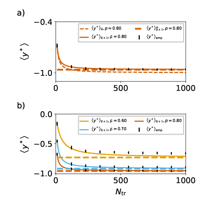
Figure (3) shows that the zeroth-order approximation ⟨y∗⟩0\left\langle y^{*}\right\rangle_{0}, even though it is able to capture some dependence on the amount of training data, is indeed too optimistic and predicts a mean-inferred network output closer to its negative target value y=−1y=-1 than numerically obtained. The first-order correction on the other hand is able to reliably predict the results. Furthermore the limiting results D→∞D\rightarrow\infty match the numerical results for different task settings pp. These limiting results are consistently higher than the zeroth-order approximation ⟨y∗⟩0\left\langle y_{*}\right\rangle_{0} and depend on the level of data variability. Deviations of the empirical results from the theory in the case p=0.6p=0.6 could stem from the fact that for p=0p=0.5 the fluctuations are maximal and our theory assumes small fluctuations.
Refer to caption
Figure 3: Predictive mean in linear regression with heterogeneous kernel. (a) Comparison of empirical data (bars), zeroth-order approximation ⟨y∗⟩0\left\langle y^{*}\right\rangle_{0} (dashed), first-order corrections ⟨y∗⟩0+1\left\langle y^{*}\right\rangle_{0+1} (solid) and the asymptotic value ⟨y∗⟩0+1∞\left\langle y^{*}\right\rangle_{0+1}^{\infty} in the case of infinite training data (dashed horizontal line) for a 1-layer linear network with σv2=1,σreg2=0.8,Ndim=50,p=0.8\sigma_{v}^{2}=1,\sigma_{\mathrm{reg}}^{2}=0.8,N_{\mathrm{dim}}=50,p=0.8. (b) Comparison of empirical inference data (bars) with first-order results ⟨y∗⟩0+1\left\langle y^{*}\right\rangle_{0+1} (solid line) and asymptotic values ⟨y∗⟩0+1∞\left\langle y^{*}\right\rangle_{0+1}^{\infty} for p=0.6p=0.6 (orange), p=0.7p=0.7 (blue) and p=0.8p=0.8 (red). Empirical results display mean and standard deviation over 50 trials with 2000 test points per trial.

III.2.2 Non-Linear Kernel

We will now investigate how the non–linearities ϕ\phi present in typical network architectures (1) influence our results for the learning curve (49) and (55).

As the ansatz in Section III.1 does not make any assumption, apart from Gaussianity, on the overlap-matrix KyK^{y}, the results presented in Section III.1.5 are general. One can use the knowledge of the statistics of the overlap matrix in the read-in layer K0K^{0} in (15) to extend the result (49) to both non-linear and deep feed-forward neural networks.

As in Section III.2.1 we start with the assumption that the input kernel matrix is distributed according to a multivariate Gaussian: Kα​β0∼𝒩⁡(μα​β,Σ(α​β)​(γ​δ))K_{\alpha\beta}^{0}\sim\mathcal{N}(\mu_{\alpha\beta},\Sigma_{(\alpha\beta)(\gamma\delta)}). In the non-linear case, we consider a read-in layer 𝐕∈ℝNh×Ndim;Vi,j∼𝒩⁡(0,σv2/Ndim)\mathbf{V}\in\mathbb{R}^{N_{h}\times N_{\mathrm{dim}}};V_{i,j}\sim\mathcal{N}\left(0,\sigma_{v}^{2}/N_{\mathrm{dim}}\right), which maps the inputs to the hidden-state space and a separate read-out layer 𝐖∈ℝ1×Nh;Wi∼𝒩⁡(0,σw2/Nh)\mathbf{W}\in\mathbb{R}^{1\times N_{h}};W_{i}\sim\mathcal{N}\left(0,\sigma_{w}^{2}/N_{h}\right), obtaining a neural network with a single hidden layer

hα(0)\displaystyle h_{\alpha}^{(0)} =𝐕​xα,\displaystyle=\mathbf{V}x_{\alpha}\,,
yα\displaystyle y_{\alpha} =𝐖​ϕ​(hα(0))+ξα,\displaystyle=\mathbf{W}\phi\left(h_{\alpha}^{(0)}\right)+\xi_{\alpha}\,, (60)

and network kernel

⟨yα​yβ⟩𝐕,𝐖\displaystyle\left\langle y_{\alpha}y_{\beta}\right\rangle_{\mathbf{V,\mathbf{W}}} =σw2Nh​∑i=1Nh⟨ϕ⁡(hα​i(0))​ϕ​(hβ​i(0))⟩𝐕\displaystyle=\frac{\sigma_{w}^{2}}{N_{h}}\text{$\sum_{i=1}^{N_{h}}\left\langle\phi\left(h_{\alpha i}^{(0)}\right)\phi\left(h_{\beta i}^{(0)}\right)\right\rangle_{\mathbf{V}}$}
+δα​β​σreg2.\displaystyle+\delta_{\alpha\beta}\,\sigma_{\mathrm{reg}}^{2}\,. (61)

As we consider the limit Nh→∞N_{h}\rightarrow\infty, one can replace the empirical average 1Nh​∑i=1Nh…\frac{1}{N_{h}}\sum_{i=1}^{N_{h}}... with a distributional average 1Nh​∑i=1Nh…→⟨…⟩𝐡(0)\frac{1}{N_{h}}\sum_{i=1}^{N_{h}}...\rightarrow\langle...\rangle_{\mathbf{h}^{(0)}} (Poole et al. 2016; Lee et al. 2017). This yields the following result for the kernel matrix Kα​βyK_{\alpha\beta}^{y} of the multivariate Gaussian

Kα​βy\displaystyle K_{\alpha\beta}^{y} →⏟Nh→∞​σw2​⟨ϕα0​ϕβ0⟩𝐡(0),𝐕+δα​β​σreg2.\displaystyle\underbrace{\rightarrow}_{N_{h}\rightarrow\infty}\sigma_{w}^{2}\text{$\left\langle\phi_{\alpha}^{0}\phi_{\beta}^{0}\right\rangle_{\mathbf{h}^{(0)},\mathbf{V}}$}+\delta_{\alpha\beta}\,\sigma_{\mathrm{reg}}^{2}\,. (62)

where we introduced the shorthand ⟨ϕ⁡(hα(0))​ϕ​(hβ(0))⟩:=⟨ϕα0​ϕβ0⟩\left\langle\phi\left(h_{\alpha}^{(0)}\right)\phi\left(h_{\beta}^{(0)}\right)\right\rangle:=\left\langle\phi_{\alpha}^{0}\phi_{\beta}^{0}\right\rangle. The expectation over the hidden states hα(0),hβ(0)h_{\alpha}^{(0)},h_{\beta}^{(0)} is with regard to the Gaussian

(hα(0)hβ(0))∼𝒩⁡((00),(Kα​α0Kα​β0Kβ​α0Kβ​β0)),\left(\begin{array}[]{c}h_{\alpha}^{(0)}\\ h_{\beta}^{(0)}\end{array}\right)\sim\mathcal{N}\left(\left(\begin{array}[]{c}0\\ 0\end{array}\right),\left(\begin{array}[]{cc}K_{\alpha\alpha}^{0}&K_{\alpha\beta}^{0}\\ K_{\beta\alpha}^{0}&K_{\beta\beta}^{0}\end{array}\right)\right)\,, (63)

with the variance Kα​α0K_{\alpha\alpha}^{0} and the covariance Kα​β0K_{\alpha\beta}^{0} given by (10). Evaluating the Gaussian integrals in (62) is analytically possible in certain limiting cases (Williams 1998; Cho and Saul 2009). For an erf\mathrm{erf}-activation function, as a prototype of a saturating activation function, this average yields

⟨ϕα0​ϕα0⟩𝐡(0)=\displaystyle\left\langle\phi_{\alpha}^{0}\phi_{\alpha}^{0}\right\rangle_{\mathbf{h}^{(0)}}= 4π​arctan⁡(1+4​Kα​α0)−1,\displaystyle\frac{4}{\pi}\arctan\left(\sqrt{1+4K_{\alpha\alpha}^{0}}\right)-1\,, (64)
⟨ϕα0​ϕβ0⟩𝐡(0)=\displaystyle\left\langle\phi_{\alpha}^{0}\phi_{\beta}^{0}\right\rangle_{\mathbf{h}^{(0)}}= 2π​arcsin⁡(2​Kα​β01+2​Kα​α0).\displaystyle\frac{2}{\pi}\arcsin\left(\frac{2K_{\alpha\beta}^{0}}{1+2K_{\alpha\alpha}^{0}}\right)\,. (65)

Equation (62) hence provides information on how the mean overlap mα​βm_{\alpha\beta} changes due to the application of the non-linearity ϕ⁡(⋅)\phi(\cdot), fixing the parameters aa, bb, KK, vv of the general form (47) as

a(Non−lin)\displaystyle a^{(\mathrm{Non-lin)}} =Kα​αy=σw2​⟨ϕα0​ϕα0⟩𝐡(0)+σreg2,\displaystyle=K_{\alpha\alpha}^{y}=\sigma_{w}^{2}\text{$\left\langle\phi_{\alpha}^{0}\phi_{\alpha}^{0}\right\rangle_{\mathbf{h}^{(0)}}$}+\sigma_{\mathrm{reg}}^{2}\,, (66)
b(Non−lin)\displaystyle b^{(\mathrm{Non-lin)}} =Kα​βy=σw2​⟨ϕα0​ϕβ0⟩𝐡(0) .\displaystyle=K_{\alpha\beta}^{y}=\sigma_{w}^{2}\text{$\left\langle\phi_{\alpha}^{0}\phi_{\beta}^{0}\right\rangle_{\mathbf{h}^{(0)}}$ }\,. (67)

where the averages over h(0)h^{(0)} are evaluated with regard to the Gaussian (63) for ϕ⁡(x)=erf⁡(x)\phi(x)=\mathrm{erf}(x). We further require in (67) that α≠β,c⁡(α)=c⁡(β)\alpha\neq\beta,\,c(\alpha)=c(\beta).

To evaluate the corrections in (49), we also need to understand how the presence of the non-linearity ϕ⁡(x)\phi(x) shapes the parameters K,vK,v that control the variability. Under the assumption of small covariance Σ(α​β)​(γ​δ)\Sigma_{(\alpha\beta)(\gamma\delta)} one can use (65) to compute C(α​β)​(γ​δ)C_{(\alpha\beta)(\gamma\delta)} using linear response theory. As Kα​β0K_{\alpha\beta}^{0} is stochastic and provided by (20), we decompose Kα​β0K_{\alpha\beta}^{0} into a deterministic kernel μα​β\mu_{\alpha\beta} and a stochastic perturbation ηα​β∼𝒩⁡(0,Σ(α​β)​(γ​δ))\eta_{\alpha\beta}\sim\mathcal{N}\left(0,\Sigma_{(\alpha\beta)(\gamma\delta)}\right). Linearizing (67) around μα​β\mu_{\alpha\beta} via Price’s theorem (Price 1958; Schuecker et al. 2016), the stochasticity in the read-out layer yields (see Appendix .1)

C(α​β)​(γ​δ)\displaystyle C_{(\alpha\beta)(\gamma\delta)} =σw4​Kα​β(ϕ′)​Kγ​δ(ϕ′)​Σ(α​β)​(γ​δ),\displaystyle=\sigma_{w}^{4}\,K_{\alpha\beta}^{(\phi^{\prime})}\,K_{\gamma\delta}^{(\phi^{\prime})}\,\Sigma_{(\alpha\beta)(\gamma\delta)}\,, (68)
Kα​β(ϕ′)\displaystyle K_{\alpha\beta}^{(\phi^{\prime})} :=⟨ϕ′​(hα(0))​ϕ′​(hβ(0))⟩,\displaystyle:=\left\langle\phi^{\prime}\left(h_{\alpha}^{(0)}\right)\phi^{\prime}\left(h_{\beta}^{(0)}\right)\right\rangle\,, (69)

where h(0)h^{(0)} is distributed as in (63). This clearly shows that the variability simply transforms with a prefactor

K(Non−lin)\displaystyle K^{(\mathrm{Non-lin)}} =σw4​Kα​β(ϕ′)​Kα​β(ϕ′)​κ,\displaystyle=\sigma_{w}^{4}\,K_{\alpha\beta}^{(\phi^{\prime})}\,K_{\alpha\beta}^{(\phi^{\prime})}\,\kappa\,, (70)
v(Non−lin)\displaystyle v^{(\mathrm{Non-lin)}} =σw4​Kα​β(ϕ′)​Kα​δ(ϕ′)​v,\displaystyle=\sigma_{w}^{4}K_{\alpha\beta}^{(\phi^{\prime})}\,K_{\alpha\delta}^{(\phi^{\prime})}\,v\,, (71)

with κ,ν\kappa,\nu defined as in (15). Evaluating the integral in ⟨ϕ′​(hα(0))​ϕ′​(hβ(0))⟩\left\langle\phi^{\prime}\left(h_{\alpha}^{(0)}\right)\phi^{\prime}\left(h_{\beta}^{(0)}\right)\right\rangle is hard in general. In fact, the integral which occurs is equivalent to the one in (Molgedey et al. 1992) for the Lyapunov exponent and, equivalently, in (Poole et al. 2016; Schoenholz et al. 2017) for the susceptibility in the propagation of information in deep feed-forward neural networks. This is consistent with the assumption that our treatment of the non-linearity follows a linear response approach as in (Molgedey et al. 1992). For the erf\mathrm{erf}-activation we can evaluate the kernel Kα​β(ϕ′)K_{\alpha\beta}^{(\phi^{\prime})} as

Kα​β(ϕ′)\displaystyle K_{\alpha\beta}^{(\phi^{\prime})} =4π⁡(1+2​a(0))​(1−(2​b(0)1+2​a(0))2)−12,\displaystyle=\frac{4}{\pi\left(1+2a^{(0)}\right)}\left(1-\left(\frac{2b^{(0)}}{1+2a^{(0)}}\right)^{2}\right)^{-\frac{1}{2}}\,, (72)
a(0)\displaystyle a^{(0)} =σv2,b(0)=σv2​u,\displaystyle=\sigma_{v}^{2}\quad,\quad b^{(0)}=\sigma_{v}^{2}u\,, (73)
u\displaystyle u =4​p​(p−1)+1,\displaystyle=4p(p-1)+1\,, (74)

which allows us to evaluate (71). Already in the one hidden-layer setting we can see that the behavior is qualitatively different from a linear setting: K(Non−lin)K^{(\mathrm{Non-lin)}} and v(Non−lin)v^{(\mathrm{Non-lin)}} scale with a linear factor which now also involves the parameter σv2\sigma_{v}^{2} in a non–linear manner.

Refer to caption
Figure 4: Predictive mean in a deep non-linear feed forward network with heterogeneous kernel. (a) Comparison of mean inferred network output for non-linear network with ϕ⁡(x)=erf⁡(x)\phi(x)=\mathrm{erf(x)}, five layers for different values of the gain σw\sigma_{w}. The figure displays numerical results (bars), zeroth-order approximation (dashed) and first-order corrections (solid). (b) Similar comparison as in (a) for different network depths L=5,10,20,50L=5,10,20,50. In all settings we used Ndim=50N_{\mathrm{dim}}=50 for D=100D=100, p=0.8p=0.8, σv2=1\sigma_{v}^{2}=1, σreg2=1\sigma_{\mathrm{reg}}^{2}=1. Empirical results display mean and standard deviation over 1000 trials with 1000 test points per trial.

III.2.3 Multilayer-Kernel

So far we considered single-layer networks. However, in practice the application of multi-layer networks is often necessary. One can straightforwardly extend the results from the non-linear case (III.2.2) to the deep non-linear case. We consider the architecture introduced in (1) in Section II.1.1 where the variable LL denotes the number of hidden layers, and 1≤l≤L1\leq l\leq L is the layer index. Similar to the computations in Section III.2.2 one can derive a set of relations to obtain Kα​βyK_{\alpha\beta}^{y}

Kα​β0\displaystyle K_{\alpha\beta}^{0} =σv2Ndim​Kα​βx,\displaystyle=\frac{\sigma_{v}^{2}}{N_{\mathrm{dim}}}\,K_{\alpha\beta}^{x}\,, (75)
Kα​β(ϕ)​l\displaystyle K_{\alpha\beta}^{(\phi)l} =σw2​⟨ϕ⁡(hα(l−1))​ϕ​(hβ(l−1))⟩,\displaystyle=\sigma_{w}^{2}\,\left\langle\phi\left(h_{\alpha}^{(l-1)}\right)\phi\left(h_{\beta}^{(l-1)}\right)\right\rangle\,, (76)
Kα​βy\displaystyle K_{\alpha\beta}^{y} =σu2​⟨ϕ⁡(hα(L))​ϕ​(hβ(L))⟩+δα​β​σreg2.\displaystyle=\sigma_{u}^{2}\,\left\langle\phi\left(h_{\alpha}^{(L)}\right)\phi\left(h_{\beta}^{(L)}\right)\right\rangle+\delta_{\alpha\beta}\,\sigma_{\mathrm{reg}}^{2}\,. (77)

with the setting K0∼𝒩⁡(μ,Σ)K^{0}\sim\mathcal{N}(\mu,\Sigma). As (Xiao et al. 2019; Poole et al. 2016; Schoenholz et al. 2017) showed for feed-forward networks, deep non-linear networks strongly alter both the variance and the covariance. So we expect them to influence the generalization properties. In order to understand how the fluctuations Σ(α​β)​(γ​δ)\Sigma_{(\alpha\beta)(\gamma\delta)} transform through propagation, one can employ the chain rule to linearize (77) and obtain

C(α​β)​(γ​δ)=σu4∏l=1L+1[Kα​β(ϕ′)​lKγ​δ(ϕ′)​l]Σ.(α​β)​(γ​δ)C_{(\alpha\beta)(\gamma\delta)}=\sigma_{u}^{4}\,\prod_{l=1}^{L+1}\left[K_{\alpha\beta}^{(\phi^{\prime})l}K_{\gamma\delta}^{(\phi^{\prime})l}\right]\,\Sigma{}_{(\alpha\beta)(\gamma\delta)}\,. (78)

A systematic derivation of this result as the leading order fluctuation correction in Nh−1N_{h}^{-1} is found in the appendix of (Segadlo et al. 2022) whereas a derivation using a linear response approach is part of Appendix .1.

Equation (77) and (78) show that the kernel performance will depend on the non-linearity ϕ\phi, the variances σv2\sigma_{v}^{2}, σw2\sigma_{w}^{2}, σu2\sigma_{u}^{2}, and the network depth LL.

Figure 4 (a) shows the comparison of the mean inferred network output ⟨y∗⟩\left\langle y^{*}\right\rangle for the true test label y=−1y=-1 between empirical results and the first order corrections. The regime (σw2<1\sigma_{w}^{2}<1) in which the kernel vanishes, leads to a poor performance. The marginal regime (σw2≃1\sigma_{w}^{2}\simeq 1) provides a better choice for the overall network performance. Equation (4) (b) shows that the maximum absolute value for the predictive mean is achieved slightly in the supercritical regime σw2>1\sigma_{w}^{2}>1. With larger number of layers, the optimum becomes more and more pronounced and approaches the critical value σw2=1\sigma_{w}^{2}=1 from above. The optimum for the predictive mean to occur slightly in the supercritical regime may be surprising with regard to the expectation that network trainability peaks precisely at σw2=1\sigma_{w}^{2}=1 (Poole et al. 2016). In particular at shallow depths, the optimum becomes very wide and shifts to σw>1\sigma_{w}>1. For few layers, even at σw2>1\sigma_{w}^{2}>1 the increase of variance Kα​αyK_{\alpha\alpha}^{y} per layer remains moderate and stays within the dynamical range of the activation function. Thus differences in covariance are faithfully transmitted by the kernel and hence allow for accurate predictions. The theory including corrections to linear order throughout matches the empirical results and hence provides good estimates for choosing the kernel architecture.

III.2.4 Experiments on Non-Symmetric Task Settings and MNIST

In contrast to the symmetric setting in the previous subsections, real data-sets such as MNIST exhibit asymmetric statistics so that the different blocks in mα​βm_{\alpha\beta} and C(α​β)​(γ​δ)C_{(\alpha\beta)(\gamma\delta)} assume different values in general. All theoretical results from Section III.1 still hold. However, as the tensor elements of mα​βm_{\alpha\beta} and C(α​β)​(γ​δ)C_{(\alpha\beta)(\gamma\delta)} change, one needs to reconsider the evaluation in Section III.1.5 in the most general form which yields a more general version of the result.

Finite MNIST dataset

First we consider a setting, where we work with the pure MNIST dataset for two distinct labels 00 and 44. In this setting we estimate the class-dependent tensor elements mα​βm_{\alpha\beta} and C(α​β)​(γ​δ)C_{(\alpha\beta)(\gamma\delta)} directly from the data. We define the data-set size per class, from which we sample the theory as DbaseD_{\mathrm{base}}. The training points are also drawn from a subset of these DbaseD_{\mathrm{base}} data points. To compare the analytical learning curve for ⟨y∗⟩\langle y_{*}\rangle at DD training data-points to the empirical results, we need to draw multiple samples of training datasets of size D<DbaseD<D_{\mathrm{base}}. As the amount of data in MNIST is limited, these samples will generally not be independent and therefore violate our assumption. Nevertheless we can see in Figure 5 that if DD is sufficiently small compared to DbaseD_{\mathrm{base}}, the empirical results and theoretical results match well.

Refer to caption
Figure 5: Predictive mean for a linear network with MNIST data: Comparison of mean inferred network output for a linear network with 1 layer for different training set sizes DD. The figure displays numerical results (bars), zeroth-order prediction (dashed) and first-order corrections (solid). Settings Ndim=784N_{\mathrm{dim}}=784, σreg2=2\sigma_{\mathrm{reg}}^{2}=2, Dbase=4000D_{\mathrm{base}}=4000. MNIST classes c1=0c_{1}=0, c2=4c_{2}=4, yc1=−1y_{c_{1}}=-1, yc2=1y_{c_{2}}=1; balanced data-set in DbaseD_{\mathrm{base}} and at each DD. Empirical results display mean and standard deviation over 10001000 trials with 10001000 test points per trial.
Gaussianized MNIST dataset

To test whether deviations in Figure 5 at large DD stem from correlations in the samples of the dataset we construct a generative scheme for MNIST data. This allows for the generation of infinitely many training points and hence the assumption that the training data is i.i.d. is fulfilled. We construct a pixel-wise Gaussian distribution for MNIST images from the samples. We use this model to sample as many MNIST images as necessary for the evaluation of the empirical learning curves. Based on the class-dependent statistics for the pixel means and the pixel covariances in the input data one can directly compute the elements of the mean μα​β\mu_{\alpha\beta} and the covariance Σ(α​β)​(γ​δ)\Sigma_{(\alpha\beta)(\gamma\delta)} for the distribution of the input kernel matrix Kα​β0K_{\alpha\beta}^{0}. We see in Figure 6 that our theory describes the results well for this data-set also for large numbers of training samples.

Furthermore we can see that in the case of an asymmetric data-set the learning curves depend on the balance ratio of training data ρ=D1/D2\rho=D_{1}/D_{2}. The bias towards class one in Figure 6 b) is evident from the curves with ρ>0.5\rho>0.5 predicting a lower mean inferred network output, closer to the target label y=−1y=-1 of class 1.

Refer to caption
Figure 6: Predictive mean for a erf-network with Gaussianized MNIST data: a) Mean inferred network output for MNIST classification with ϕ⁡(x)=erf⁡(x)\phi(x)=\mathrm{erf(x)}. Figure shows zeroth-order (dashed line), first-order (solid line), and empirical results (bars). b) Mean inferred network output in first order approximation (solid lines) and empirical results (bars) for MNIST classification with different ratios ρ=D1/D2\rho=D_{1}/D_{2} between numbers of training samples per class D1D_{1} and D2D_{2}, respectively; ρ=0.5\rho=0.5 (yellow), ρ=0.6\rho=0.6 (blue), ρ=0.7\rho=0.7 (red). Empirical results display mean and standard deviation over 50 trials with 1000 test points per trial.

IV Discussion

In this work we investigate the influence of data variability on the performance of Bayesian inference. The probabilistic nature of the data manifests itself in a heterogeneity of the entries in the block-structured kernel matrix of the corresponding Gaussian process. We show that this heterogeneity for a sufficiently large number of DD of data samples can be treated as an effective non-Gaussian theory. By employing a time-dependent formulation for the mean of the predictive distribution, this heterogeneity can be treated as a disorder average that circumvents the use of the replica trick; which was the basis of previous investigations of analytical learning curves (Malzahn and Opper 2001). A perturbative treatment of the variability yields first-order corrections to the mean in the variance of the heterogeneity that always push the mean of the predictive distribution towards zero. In particular, we obtain limiting expressions that accurately describe the mean in the limit of infinite training data, qualitatively correcting the zeroth-order approximation corresponding to homogeneous kernel matrices, is overconfident in predicting the mean to perfectly match the training data in this limit. This finding shows how variability fundamentally limits predictive performance and provides not only a quantitative but also a qualitative difference. Moreover at a finite number of training data the theory explains the empirically observed performance accurately. We show that our framework captures predictions in linear, non-linear shallow and deep networks. In non-linear networks, we show that the optimal value for the variance of the prior weight distribution is achieved in the super-critical regime. The optimal range for this parameter is broad in shallow networks and becomes progressively more narrow in deep networks. These findings support that the optimal initialization is not at the critical point where the variance is unity, as previously thought (Poole et al. 2016), but that super-critical initialization may have an advantage when considering input variability. An artificial dataset illustrates the origin and the typical statistical structure that arises in heterogeneous kernels, while the application of the formalism to MNIST (LeCun et al. 1998) demonstrates potential use to predict the expected performance in real world applications.

The field theoretical formalism can be combined with approaches that study the effect of fluctuations due to the finite width of the layers (Naveh et al. 2020; Yaida 2020; Zavatone-Veth et al. 2021; Segadlo et al. 2022). In fact, in the large NhN_{h} limit the NNGP kernel is inert to the training data, the so called lazy regime. At finite network width, the kernel itself receives corrections which are commonly associated with the adaptation of the network to the training data, thus representing what is known as feature learning. The interplay of heterogeneity of the kernel with such finite-size adaptations is a fruitful future direction.

Another approach to study learning in the limit of large width is offered by the neural tangent kernel (NTK) (Jacot et al. 2018), which considers the effect of gradient descent on the network output up to linear order in the change of the weights. A combination of the approach presented here with the NTK instead of the NNGP kernel seems possible and would provide insights into how data heterogeneity affects training dynamics.

The analytical results presented here are based on the assumption that the variability of the data is small and can hence be treated perturbatively. In the regime of large data variability, it is conceivable to employ self-consistent methods instead, which would technically correspond to the computation of saddle points of certain order parameters, which typically leads to an infinite resummation of the perturbative terms that dominate in the large NhN_{h} limit. Such approaches may be useful to study and predict the performance of kernel methods for data that show little or no linear separability and are thus dominated by variability. Another direction of extension is the computation of the variance of the Bayesian predictor, which in principle can be treated with the same set of methods as presented here. Finally, since the large width limit as well as finite-size corrections, which in particular yield the kernel response function that we employed here, can be obtained for recurrent and deep networks in the same formalism (Segadlo et al. 2022) as well as for residual networks (ResNets) (Fischer et al. 2023), the theory of generalization presented here can straight forwardly be extended to recurrent networks and to ResNets.

We intend to upload the source code to produce the figures in the manuscript to Zenodo.

Acknowledgments

We thank Claudia Merger, Bastian Epping, Kai Segadlo, Alexander van Meegen and Noah Schürholz for helpful discussions. This work was partly supported by the German Federal Ministry for Education and Research (BMBF Grant 01IS19077A to Jülich and BMBF Grant 01IS19077B to Aachen) and funded by the Deutsche Forschungsgemeinschaft (DFG, German Research Foundation) - 368482240/GRK2416, the Excellence Initiative of the German federal and state governments (ERS PF-JARA-SDS005), and the Helmholtz Association Initiative and Networking Fund under project number SO-092 (Advanced Computing Architectures, ACA). Open access publication funded by the Deutsche Forschungsgemeinschaft (DFG, German Research Foundation) – 491111487.

References

  • Sompolinsky et al. (1988) H. Sompolinsky, A. Crisanti, and H. J. Sommers, Chaos in random neural networks, Phys. Rev. Lett. 61, 259 (1988).
  • Amit et al. (1985) D. J. Amit, H. Gutfreund, and H. Sompolinsky, Storing infinite numbers of patterns in a spin-glass model of neural networks, Phys. Rev. Lett. 55, 1530 (1985).
  • Gardner (1988) E. Gardner, The space of interactions in neural network models, J. Phys. A Math. Gen. 21, 257 (1988).
  • Gardner and Derrida (1988) E. Gardner and B. Derrida, Optimal storage properties of neural network models, J. Phys. A Math. Gen. 21, 271 (1988).
  • Neal (1996) R. M. Neal, Bayesian Learning for Neural Networks (Springer New York, 1996).
  • Williams (1996) C. Williams, Computing with infinite networks, in Adv. Neural Inf. Process. Syst., Vol. 9, edited by M. Mozer, M. Jordan, and T. Petsche (MIT Press, 1996).
  • Poole et al. (2016) B. Poole, S. Lahiri, M. Raghu, J. Sohl-Dickstein, and S. Ganguli, Exponential expressivity in deep neural networks through transient chaos, in Advances in Neural Information Processing Systems 29 (2016).
  • Schoenholz et al. (2017) S. S. Schoenholz, J. Gilmer, S. Ganguli, and J. Sohl-Dickstein, Deep information propagation, 5th International Conference on Learning Representations, ICLR 2017 - Conference Track Proceedings (2017), 10.48550/arxiv.1611.01232, arXiv:1611.01232 .
  • Yang (2019) G. Yang, Wide feedforward or recurrent neural networks of any architecture are gaussian processes, in Adv. Neural Inf. Process. Syst., Vol. 32, edited by H. Wallach, H. Larochelle, A. Beygelzimer, F. d'Alché-Buc, E. Fox, and R. Garnett (Curran Associates, Inc., 2019).
  • Cui et al. (2022) H. Cui, B. Loureiro, F. Krzakala, and L. Zdeborová, Generalization error rates in kernel regression: the crossover from the noiseless to noisy regime, Journal of Statistical Mechanics: Theory and Experiment 2022, 114004 (2022).
  • Ruben and Pehlevan (2023) B. S. Ruben and C. Pehlevan, Learning curves for heterogeneous feature-subsampled ridge ensembles, ArXiv (2023).
  • Jacot et al. (2018) A. Jacot, F. Gabriel, and C. Hongler, Neural tangent kernel: Convergence and generalization in neural networks, in Advances in Neural Information Processing Systems 31 (2018) pp. 8580–8589.
  • Cohen et al. (2021) O. Cohen, O. Malka, and Z. Ringel, Learning curves for overparametrized deep neural networks: A field theory perspective, Phys. Rev. Res. 3, 023034 (2021).
  • Naveh and Ringel (2021) G. Naveh and Z. Ringel, A self consistent theory of gaussian processes captures feature learning effects in finite CNNs, in Adv. Neural Inf. Process. Syst., edited by A. Beygelzimer, Y. Dauphin, P. Liang, and J. W. Vaughan (2021).
  • Zavatone-Veth and Pehlevan (2021) J. A. Zavatone-Veth and C. Pehlevan, Exact marginal prior distributions of finite bayesian neural networks, in Adv. Neural Inf. Process. Syst., edited by A. Beygelzimer, Y. Dauphin, P. Liang, and J. W. Vaughan (2021).
  • Zavatone-Veth et al. (2021) J. A. Zavatone-Veth, A. Canatar, B. Ruben, and C. Pehlevan, Asymptotics of representation learning in finite bayesian neural networks, in Adv. Neural Inf. Process. Syst., edited by A. Beygelzimer, Y. Dauphin, P. Liang, and J. W. Vaughan (2021).
  • Li and Sompolinsky (2021) Q. Li and H. Sompolinsky, Statistical Mechanics of Deep Linear Neural Networks: The Backpropagating Kernel Renormalization, Phys. Rev. X 11, 031059 (2021).
  • Roberts et al. (2022) D. A. Roberts, S. Yaida, and B. Hanin, The Principles of Deep Learning Theory (Cambridge University Press, 2022).
  • Bordelon and Pehlevan (2022) B. Bordelon and C. Pehlevan, Self-consistent dynamical field theory of kernel evolution in wide neural networks, in Advances in Neural Information Processing Systems, Vol. 35, edited by S. Koyejo, S. Mohamed, A. Agarwal, D. Belgrave, K. Cho, and A. Oh (Curran Associates, Inc., 2022) pp. 32240–32256.
  • Murphy (2023) K. P. Murphy, Probabilistic Machine Learning: Advanced Topics (MIT Press, 2023).
  • LeCun et al. (1998) Y. LeCun, C. Cortes, and C. J. Burges, The mnist database of handwritten digits, (1998).
  • MacKay (2003) D. J. MacKay, Information theory, inference and learning algorithms (Cambridge university press, 2003).
  • Murphy (2022) K. P. Murphy, Probabilistic Machine Learning: An introduction (MIT Press, 2022).
  • Williams and Barber (1998) C. K. I. Williams and D. Barber, Bayesian classification with gaussian processes, IEEE Trans. Pattern Anal. Mach. Intel. 20, 1342 (1998).
  • Rasmussen and Williams (2006) C. Rasmussen and C. Williams, Gaussian Processes for Machine Learning, Adaptive Computation and Machine Learning (MIT Press, Cambridge, MA, USA, 2006) p. 248.
  • Cho and Saul (2009) Y. Cho and L. Saul, Kernel methods for deep learning, in Adv. Neural Inf. Process. Syst., Vol. 22, edited by Y. Bengio, D. Schuurmans, J. Lafferty, C. Williams, and A. Culotta (Curran Associates, Inc., 2009).
  • Lee et al. (2018) J. Lee, J. Sohl-Dickstein, J. Pennington, R. Novak, S. Schoenholz, and Y. Bahri, Deep neural networks as gaussian processes, in International Conference on Learning Representations (2018).
  • Segadlo et al. (2022) K. Segadlo, B. Epping, A. van Meegen, D. Dahmen, M. Krämer, and M. Helias, Unified field theoretical approach to deep and recurrent neuronal networks, J. Stat. Mech. Theory Exp. 2022, 103401 (2022).
  • Ariosto et al. (2023) S. Ariosto, R. Pacelli, M. Pastore, F. Ginelli, M. Gherardi, and P. Rotondo, Statistical mechanics of deep learning beyond the infinite-width limit, ArXiv (2023), 2209.04882 .
  • Hoerl and Kennard (2000) A. E. Hoerl and R. W. Kennard, Ridge regression: Biased estimation for nonorthogonal problems, Technometrics 42, 80 (2000).
  • Williams and Rasmussen (2006) C. K. Williams and C. E. Rasmussen, Gaussian Processes for Machine Learning, 1st ed. (MIT Press, Cambridge, 2006).
  • Goodfellow et al. (2016) I. Goodfellow, Y. Bengio, and A. Courville, Deep Learning (MIT Press, 2016) http://www.deeplearningbook.org.
  • Fischer and Hertz (1991) K. Fischer and J. Hertz, Spin glasses (Cambridge University Press, 1991).
  • Mezard and Montanari (2009) M. Mezard and A. Montanari, Information, physics and computation (Oxford University Press, 2009).
  • De Dominicis (1978) C. De Dominicis, Dynamics as a substitute for replicas in systems with quenched random impurities, Phys. Rev. B 18, 4913 (1978).
  • Martin et al. (1973) P. Martin, E. Siggia, and H. Rose, Statistical dynamics of classical systems, Phys. Rev. A 8, 423 (1973).
  • Janssen (1976) H.-K. Janssen, On a lagrangean for classical field dynamics and renormalization group calculations of dynamical critical properties, Z. Phys. B 23, 377 (1976).
  • Stapmanns et al. (2020) J. Stapmanns, T. Kühn, D. Dahmen, T. Luu, C. Honerkamp, and M. Helias, Self-consistent formulations for stochastic nonlinear neuronal dynamics, Phys. Rev. E 101, 042124 (2020).
  • Helias and Dahmen (2020) M. Helias and D. Dahmen, Statistical Field Theory for Neural Networks (Springer International Publishing, 2020) p. 203.
  • Zinn-Justin (1996) J. Zinn-Justin, Quantum field theory and critical phenomena (Clarendon Press, Oxford, 1996).
  • Ensslin and Frommert (2010) T. Ensslin and M. Frommert, Reconstruction of signals with unknown spectra in information field theory with parameter uncertainty, Physical Review D - Particles, Fields, Gravitation and Cosmology 83 (2010), 10.1103/PhysRevD.83.105014, 1002.2928v3 .
  • Dyer and Gur-Ari (2019) E. Dyer and G. Gur-Ari, Asymptotics of Wide Networks from Feynman Diagrams, ArXiv (2019).
  • Fischer et al. (2022) K. Fischer, A. René, C. Keup, M. Layer, D. Dahmen, and M. Helias, Decomposing neural networks as mappings of correlation functions, Phys. Rev. Res. 4, 043143 (2022).
  • Segadlo (2021) K. Segadlo, Theory of learning and prediction by deep and recurrent networks in Gaussian process approximation, Master’s thesis, RWTH Aachen University (2021).
  • Lee et al. (2017) J. Lee, Y. Bahri, R. Novak, S. S. Schoenholz, J. Pennington, and J. Sohl-Dickstein, Deep neural networks as gaussian processes, ArXiv , 1711.00165 (2017), arXiv:1711.00165 .
  • Williams (1998) C. K. Williams, Computation with infinite neural networks, Neural Comput. 10, 1203 (1998).
  • Price (1958) R. Price, A useful theorem for nonlinear devices having gaussian inputs, IRE Trans. Inf. Theory 4, 69 (1958).
  • Schuecker et al. (2016) J. Schuecker, S. Goedeke, D. Dahmen, and M. Helias, Functional methods for disordered neural networks, ArXiv (2016), 10.48550/arXiv.1605.06758, 1605.06758 [cond-mat.dis-nn].
  • Molgedey et al. (1992) L. Molgedey, J. Schuchhardt, and H. Schuster, Suppressing chaos in neural networks by noise, Phys. Rev. Lett. 69, 3717 (1992).
  • Xiao et al. (2019) L. Xiao, J. Pennington, and S. S. Schoenholz, Disentangling trainability and generalization in deep neural networks, in International Conference on Machine Learning (2019).
  • Malzahn and Opper (2001) D. Malzahn and M. Opper, A variational approach to learning curves, in Advances in Neural Information Processing Systems, Vol. 14, edited by T. Dietterich, S. Becker, and Z. Ghahramani (MIT Press, 2001).
  • Naveh et al. (2020) G. Naveh, O. Ben-David, H. Sompolinsky, and Z. Ringel, Predicting the outputs of finite networks trained with noisy gradients, ArXiv (2020).
  • Yaida (2020) S. Yaida, Non-Gaussian processes and neural networks at finite widths, in Proceedings of The First Mathematical and Scientific Machine Learning Conference, Proceedings of Machine Learning Research, Vol. 107, edited by J. Lu and R. Ward (PMLR, Princeton University, Princeton, NJ, USA, 2020) pp. 165–192.
  • Fischer et al. (2023) K. Fischer, D. Dahmen, and M. Helias, Optimal signal propagation in ResNets through residual scaling, ArXiv (2023), 2305.07715 .

Appendices

.1 The dynamic moment generating function Z⁡(L∗,Ky)Z(L_{*},K^{y})

Ultimately we want to compute the disorder-average of

y∗​(K∗⁣⋅,K⋅⁣⋅)\displaystyle y_{*}\left(K_{*\cdot},K_{\cdot\cdot}\right) =K∗α​Kα​β−1​yβ,\displaystyle=K_{*\alpha}K_{\alpha\beta}^{-1}y_{\beta}\,, (A1)
⟨y∗⟩K∗⁣⋅,K⋅⁣⋅\displaystyle\left\langle y_{*}\right\rangle_{K_{*\cdot},K_{\cdot\cdot}} =⟨K∗α​Kα​β−1​yβ⟩K∗⁣⋅,K⋅⁣⋅,\displaystyle=\left\langle K_{*\alpha}K_{\alpha\beta}^{-1}y_{\beta}\right\rangle_{K_{*\cdot},K_{\cdot\cdot}}\,, (A2)

where Kα​β,K∗αK_{\alpha\beta},K_{*\alpha} indicate the kernel matrix of training samples and the kernel matrix between test and training samples, respectively. As the matrices K∗α,Kα​βK_{*\alpha},K_{\alpha\beta} are correlated (due to the presence of the same training data in both matrices) and Kα​βK_{\alpha\beta} occurs as a inverse, the average is not straightforward. One way to evaluate (A2) is to compute the average of the moment generating function Z⁡(j)Z(j) of the predictive distribution and to compute its derivatives. By (3) the predictive distribution is given by the ratio of p(y∗,𝐲tr|x∗,𝐱tr)p\left(y_{*},\mathbf{y}_{\mathrm{tr}}|x_{*},\mathbf{x}_{\mathrm{tr}}\right) and p⁡(𝐲tr|𝐱tr)p\left(\mathbf{y}_{\mathrm{tr}}|\mathbf{x}_{\mathrm{tr}}\right), which each describe a Gaussian process with a simple dependence on KK (Segadlo et al. 2022). Consequently, the moment generating function of the predictive distribution is also given as a ratio

⟨Z⁡(j)⟩K=⟨𝒵⁡(j,K)𝒵⁡(0,K)⟩K,\left\langle Z(j)\right\rangle_{K}=\left\langle\frac{\mathcal{Z}(j,K)}{\mathcal{Z}(0,K)}\right\rangle_{K}\,, (A3)

which requires an average over the numerator and the denominator, which are also correlated as the normalization 𝒵⁡(0,K)\mathcal{Z}(0,K) also depends on the realization of KK. We hence introduce a dynamic approach, where the normalization 𝒵⁡(0,K)\mathcal{Z}(0,K) is fixed by construction to 𝒵⁡(0,K)=1​∀K\mathcal{Z}(0,K)=1\>\forall K (De Dominicis 1978). We define the dynamics of an auxiliary variable qα​(t)q_{\alpha}(t) via

∂∂t​qα​(t)=−Kα​β​qβ​(t)+yα.\frac{\partial}{\partial t}q_{\alpha}(t)=-K_{\alpha\beta}q_{\beta}(t)+y_{\alpha}\,. (A4)

This inhomogeneous differential equation in the long time limit converges to

qα​(t→∞)\displaystyle q_{\alpha}(t\rightarrow\infty) =Kα​β−1​yβ.\displaystyle=K_{\alpha\beta}^{-1}y_{\beta}\,. (A5)

We used the fact that Kα​βK_{\alpha\beta} is positive semi-definite, as it is a covariance matrix. It is hence safe to assume that a fixed point qα​(t→∞)q_{\alpha}(t\rightarrow\infty) exists. Further we make the assumption, that we start the dynamics at t→−∞t\rightarrow-\infty with an arbitrary initial condition. Hence we can assume that the fixed point is achieved. A readout of qα​(t→∞)q_{\alpha}(t\rightarrow\infty) using the test-train kernel matrix K∗αK_{*\alpha} yields the mean inferred network output (A1) for a fixed realization of K∗α,Kα​βK_{*\alpha},K_{\alpha\beta}. We want to compute the disorder average of K∗α​qα​(t→∞)K_{*\alpha}q_{\alpha}(t\rightarrow\infty) . Using the Martin-Siggia-Rose-DeDominicis-Jannsen formalism we construct the dynamic moment generating function ZZ for the dynamics given in (A4):

Z⁡(l∗,K)\displaystyle Z(l_{*},K) =∫∏α=1Dd​q~α​exp⁡(S⁡(q,q~,K∗⁣⋅,K⋅⁣⋅,l∗)),\displaystyle=\int\prod_{\alpha=1}^{D}d\tilde{q}_{\alpha}\exp\left(S(q,\tilde{q},K_{*\cdot},K_{\cdot\cdot},l_{*})\right)\,, (A6)
S⁡(q,q~,K∗⁣⋅,K⋅⁣⋅,l∗)\displaystyle S(q,\tilde{q},K_{*\cdot},K_{\cdot\cdot},l_{*}) :=∫d​t​q~α​(t)​[∂∂t​𝕀α​β+Kα​β]​qβ​(t)−∫d​t​q~α​(t)​yα+∫d​t​l∗​(t)​K∗α​qα​(t).\displaystyle:=\int dt\tilde{q}_{\alpha}(t)\left[\frac{\partial}{\partial t}\mathbb{I}_{\alpha\beta}+K_{\alpha\beta}\right]q_{\beta}(t)-\int dt\tilde{q}_{\alpha}(t)y_{\alpha}+\int dtl_{*}(t)K_{*\alpha}q_{\alpha}(t)\ . (A7)

We now go to Fourier space in the variables qα​(t),q~α​(t)→Qα​(ω),Q~α​(ω)q_{\alpha}(t),\tilde{q}_{\alpha}(t)\rightarrow Q_{\alpha}(\omega),\tilde{Q}_{\alpha}(\omega) using the definition

qα​(t)\displaystyle q_{\alpha}(t) =12​π​∫−∞∞d​ω​exp⁡(i​ω​t)​Qα​(ω),\displaystyle=\frac{1}{2\pi}\int_{-\infty}^{\infty}d\omega\exp(i\omega t)Q_{\alpha}(\omega)\,, (A8)
Qα​(ω)\displaystyle Q_{\alpha}(\omega) =∫−∞∞d​t​exp⁡(−i​ω​t)​qα​(t).\displaystyle=\int_{-\infty}^{\infty}dt\exp(-i\omega t)q_{\alpha}(t)\,. (A9)

Consequently products in time domain transform as

∫d​t​qα​(t)​pβ​(t)\displaystyle\int dtq_{\alpha}(t)p_{\beta}(t) =12​π​∫−∞∞d​ω​Qα​(ω)​Pβ​(−ω):=Qα⊤​Pβ\displaystyle=\frac{1}{2\pi}\int_{-\infty}^{\infty}d\omega Q_{\alpha}(\omega)P_{\beta}(-\omega):=Q_{\alpha}^{\top}P_{\beta} (A10)

where we defined the inner product in Fourier domain; we here used that (2​π)−1​∫d​t​exp⁡[i​t​(ω+ω′)]=δ⁡(ω+ω′)(2\pi)^{-1}\int dt\exp\left[it\left(\omega+\omega^{\prime}\right)\right]=\delta\left(\omega+\omega^{\prime}\right). Likewise the time-derivative ∂t\partial_{t} transforms as

∫d​t​qα​(t)​∂∂t​qβ​(t)\displaystyle\int dtq_{\alpha}(t)\frac{\partial}{\partial t}q_{\beta}(t) =12​π​∫d​ω​Qα​(−ω)​i​ω​Qβ​(ω)=Qα⊤​(i​ω)​Qβ.\displaystyle=\frac{1}{2\pi}\int d\omega\,Q_{\alpha}(-\omega)i\omega Q_{\beta}(\omega)=Q_{\alpha}^{\top}(i\omega)Q_{\beta}\,. (A11)

Lastly the product ∫d​t​q~α​(t)​yα\int dt\tilde{q}_{\alpha}(t)y_{\alpha} transforms as

∫d​t​q~α​(t)​yα\displaystyle\int dt\tilde{q}_{\alpha}(t)y_{\alpha} =∫d​t​12​π​∫d​ω​exp⁡(i​ω​t)​Q~α​(ω)​yα\displaystyle=\int dt\frac{1}{2\pi}\int d\omega\exp(i\omega t)\tilde{Q}_{\alpha}(\omega)y_{\alpha} (A12)
=∫d​ω​δ​(ω)​Q~α​(ω)​yα\displaystyle=\int d\omega\delta(\omega)\tilde{Q}_{\alpha}(\omega)y_{\alpha} (A13)
=Q~α​(ω=0)​yα\displaystyle=\tilde{Q}_{\alpha}(\omega=0)y_{\alpha} (A14)

Those definitions transform the action of the dynamic moment generating functional (MGF) (A6) to

S⁡(Q,Q~,K∗⁣⋅,K⋅⁣⋅,L∗)\displaystyle S(Q,\tilde{Q},K_{*\cdot},K_{\cdot\cdot},L_{*}) =12​π​∫d​ω​d​ω′​δ​(ω+ω′)​Q~α​(ω)​[i​ω′​𝕀α​β+Kα​β]​Qβ​(ω′)−Q~α​(ω=0)​yα\displaystyle=\frac{1}{2\pi}\int d\omega d\omega^{\prime}\delta(\omega+\omega^{\prime})\tilde{Q}_{\alpha}(\omega)\left[i\omega^{\prime}\mathbb{I}_{\alpha\beta}+K_{\alpha\beta}\right]Q_{\beta}(\omega^{\prime})-\tilde{Q}_{\alpha}(\omega=0)y_{\alpha}
+12​π∫dωL∗(ω)K∗αQα(−ω).\displaystyle+\frac{1}{2\pi}\int d\omega\,L_{*}(\omega)K_{*\alpha}Q_{\alpha}(-\omega)\,. (A15)

We now want to perform the disorder average. As in the main text we assume Gaussian disorder for Kα​β,K∗αK_{\alpha\beta},\,K_{*\alpha} according to the statistics (21) and compute the disorder averaged moment generating function

⟨Z⁡(L∗,K)⟩K=∫𝒟⁡{Q​Q~}​⟨exp⁡(S⁡(Q,Q~,K∗⁣⋅,K⋅⁣⋅,L∗))⟩K.\left\langle Z(L_{*},K)\right\rangle_{K}=\int\mathcal{D}\{Q\tilde{Q}\}\left\langle\exp\left(S(Q,\tilde{Q},K_{*\cdot},K_{\cdot\cdot},L_{*})\right)\right\rangle_{K}\,. (A16)

As K∗α,Kα​βK_{*\alpha},\,K_{\alpha\beta} appear linearly in the action and both are Gaussian variables, the average is straightforward and only affects the term

⟨exp⁡(Q~α⊤​Qβ​Kα​β+K∗α​L∗⊤​Qα)⟩K\displaystyle\left\langle\exp\left(\tilde{Q}_{\alpha}^{\top}Q_{\beta}K_{\alpha\beta}+K_{*\alpha}L_{*}^{\top}Q_{\alpha}\right)\right\rangle_{K} =exp⁡(S¯),\displaystyle=\exp\left(\overline{S}\right)\,, (A17)

with

S¯\displaystyle\overline{S} =mα​β​Q~α⊤​Qβ+m∗α​L∗⊤​Qα\displaystyle=m_{\alpha\beta}\tilde{Q}_{\alpha}^{\top}Q_{\beta}+m_{*\alpha}L_{*}^{\top}Q_{\alpha} (A18)
+12​C(α​β)​(γ​δ)​Q~α⊤​Qβ​Q~γ⊤​Qδ\displaystyle+\frac{1}{2}C_{(\alpha\beta)(\gamma\delta)}\tilde{Q}_{\alpha}^{\top}Q_{\beta}\tilde{Q}_{\gamma}^{\top}Q_{\delta}
+C(∗α)(βγ)L∗⊤QαQ~β⊤Qγ+𝒪(L∗2).\displaystyle+C_{(*\alpha)(\beta\gamma)}L_{*}^{\top}Q_{\alpha}\tilde{Q}_{\beta}^{\top}Q_{\gamma}+\mathcal{O}\left(L_{*}^{2}\right)\,. (A19)

In the main text and in this appendix we only consider perturbative corrections towards the mean inferred network output. This corresponds to computing the derivative of ⟨Z⁡(L∗,K)⟩K\left\langle Z(L_{*},K)\right\rangle_{K} and subsequently setting L∗=0L_{*}=0. Because of this we only need to consider terms which are linear in L∗L_{*} and hence drop any 𝒪⁡(L∗2)\mathcal{O}\left(L_{*}^{2}\right) in A19. Hence the full disorder averaged action reads

⟨exp⁡(S⁡(Q,Q~,K∗⁣⋅,K⋅⁣⋅,L∗))⟩K\displaystyle\left\langle\exp\left(S(Q,\tilde{Q},K_{*\cdot},K_{\cdot\cdot},L_{*})\right)\right\rangle_{K} =exp⁡(Q~α⊤​[i​ω​𝕀α​β+mα​β]​Qβ−Q~α​(ω=0)​yα+m∗α​L∗⊤​QαCLOSE\displaystyle=\exp\bigg(\tilde{Q}_{\alpha}^{\top}\left[i\omega\mathbb{I}_{\alpha\beta}+m_{\alpha\beta}\right]Q_{\beta}-\tilde{Q}_{\alpha}(\omega=0)y_{\alpha}+m_{*\alpha}L_{*}^{\top}Q_{\alpha}
+12C(α​β)​(γ​δ)Q~α⊤QβQ~γ⊤Qδ+C(∗α)(βγ)L∗⊤QαQ~β⊤Qγ).\displaystyle+\frac{1}{2}C_{(\alpha\beta)(\gamma\delta)}\tilde{Q}_{\alpha}^{\top}Q_{\beta}\tilde{Q}_{\gamma}^{\top}Q_{\delta}+C_{(*\alpha)(\beta\gamma)}L_{*}^{\top}Q_{\alpha}\tilde{Q}_{\beta}^{\top}Q_{\gamma}\bigg)\,. (A20)

We can decompose this action into a free theory with added perturbative vertices. The free theory is simply a quadratic theory in QQ and Q~\tilde{Q}

⟨exp⁡(S⁡(Q,Q~,K∗⁣⋅,K⋅⁣⋅,L∗))⟩K(0)\displaystyle\left\langle\exp\left(S(Q,\tilde{Q},K_{*\cdot},K_{\cdot\cdot},L_{*})\right)\right\rangle_{K}^{(0)} =exp⁡(Q~α⊤​[i​ω​𝕀α​β+mα​β]​Qβ−Q~α​(ω=0)​yα+m∗α​L∗⊤​Qα)\displaystyle=\exp\left(\tilde{Q}_{\alpha}^{\top}\left[i\omega\mathbb{I}_{\alpha\beta}+m_{\alpha\beta}\right]Q_{\beta}-\tilde{Q}_{\alpha}(\omega=0)y_{\alpha}+m_{*\alpha}L_{*}^{\top}Q_{\alpha}\right) (A21)
=exp⁡(−12​(Q~αQα)⊤​(0−(i​ω​𝕀α​β+mα​β)−(−i​ω​𝕀α​β+mα​β)0)​(Q~αQα)\displaystyle=\exp\bigg(-\frac{1}{2}\left(\begin{array}[]{c}\tilde{Q}_{\alpha}\\ Q_{\alpha}\end{array}\right)^{\top}\left(\begin{array}[]{cc}0&-(i\omega\mathbb{I}_{\alpha\beta}+m_{\alpha\beta})\\ -(-i\omega\mathbb{I}_{\alpha\beta}+m_{\alpha\beta})&0\end{array}\right)\left(\begin{array}[]{c}\tilde{Q}_{\alpha}\\ Q_{\alpha}\end{array}\right)
OPEN−Q~α​(ω=0)​yα+m∗α​L∗⊤​Qα).\displaystyle-\tilde{Q}_{\alpha}(\omega=0)y_{\alpha}+m_{*\alpha}L_{*}^{\top}Q_{\alpha}\bigg)\,. (A28)

whereas the perturbative part consists of expressions reminiscent of the φ3+φ4\varphi^{3}+\varphi^{4} theory

⟨exp⁡(S⁡(Q,Q~,K∗⁣⋅,K⋅⁣⋅,L∗))⟩K(1)\displaystyle\left\langle\exp\left(S(Q,\tilde{Q},K_{*\cdot},K_{\cdot\cdot},L_{*})\right)\right\rangle_{K}^{(1)} =exp⁡(12​Q~α⊤​Qβ​C(α​β)​(γ​δ)​Q~γ⊤​QδCLOSE\displaystyle=\exp\bigg(\frac{1}{2}\tilde{Q}_{\alpha}^{\top}Q_{\beta}C_{(\alpha\beta)(\gamma\delta)}\tilde{Q}_{\gamma}^{\top}Q_{\delta}
+C(∗α)(βγ)L∗⊤QαQ~β⊤Qγ+𝒪(L∗2)).\displaystyle+C_{(*\alpha)(\beta\gamma)}L_{*}^{\top}Q_{\alpha}\tilde{Q}_{\beta}^{\top}Q_{\gamma}+\mathcal{O}\left(L_{*}^{2}\right)\bigg)\,. (A29)

The fixed point dynamics in (A4) and (A5) can also be treated in the Fourier domain. From the inverse Fourier transform we obtain our limit results via

qα​(t)\displaystyle q_{\alpha}(t) =12​π​∫d​ω​exp⁡(i​ω​t)​Qα​(ω)\displaystyle=\frac{1}{2\pi}\int d\omega\exp(i\omega t)Q_{\alpha}(\omega) (A30)
⟨y∗⟩K\displaystyle\left\langle y_{*}\right\rangle_{K} =limt→∞⟨12​π​∫d​ω​exp⁡(i​ω​t)​K∗α​Qα​(ω)⟩L\displaystyle=\lim_{t\rightarrow\infty}\left\langle\frac{1}{2\pi}\int d\omega\exp(i\omega t)K_{*\alpha}Q_{\alpha}(\omega)\right\rangle_{L} (A31)
⟨y∗⟩K\displaystyle\left\langle y_{*}\right\rangle_{K} =limt→∞12​π∫dωexp(iωt)2πδδ​L∗​(−ω)[⟨Z(L∗,K)⟩K]|L∗​(ω)=0\displaystyle=\lim_{t\rightarrow\infty}\frac{1}{2\pi}\int d\omega\exp(i\omega t)2\pi\frac{\delta}{\delta L_{*}(-\omega)}\left[\left\langle Z(L_{*},K)\right\rangle_{K}\right]\bigg\rvert_{L_{*}(\omega)=0} (A32)

.1.1 The free case

In the free case the action implies that we can contract the monopoles −Q~α​(ω=0)​yα-\tilde{Q}_{\alpha}(\omega=0)y_{\alpha} and m∗α​L∗⊤​Qαm_{*\alpha}L_{*}^{\top}Q_{\alpha} with the propagator

Δα​β​(ω,ω′)\displaystyle\Delta_{\alpha\beta}(\omega,\omega^{\prime}) =(⟨Q~α​(ω)​Q~β​(ω′)⟩⟨Qα​(ω)​Q~β​(ω′)⟩⟨Q~α​(ω)​Qβ​(ω′)⟩⟨Qα​(ω)​Qβ​(ω′)⟩)\displaystyle=\left(\begin{array}[]{cc}\left\langle\tilde{Q}_{\alpha}(\omega)\tilde{Q}_{\beta}(\omega^{\prime})\right\rangle&\left\langle Q_{\alpha}(\omega)\tilde{Q}_{\beta}(\omega^{\prime})\right\rangle\\ \left\langle\tilde{Q}_{\alpha}(\omega)Q_{\beta}(\omega^{\prime})\right\rangle&\left\langle Q_{\alpha}(\omega)Q_{\beta}(\omega^{\prime})\right\rangle\end{array}\right)
=[12​π​δ​(ω+ω′)​(0−(i​ω​𝕀+m)α​β−(−i​ω​𝕀+m)α​β0)]−1\displaystyle=\left[\frac{1}{2\pi}\delta(\omega+\omega^{\prime})\left(\begin{array}[]{cc}0&-(i\omega\mathbb{I}+m)_{\alpha\beta}\\ -(-i\omega\mathbb{I}+m)_{\alpha\beta}&0\end{array}\right)\right]^{-1}
=2​π​δ(OPENω+ω′)​(0−(−i​ω​𝕀+m)α​β−1−(i​ω​𝕀+m)α​β−10).\displaystyle=2\pi\text{$\delta$($\omega+\omega^{\prime})$}\left(\begin{array}[]{cc}0&-(-i\omega\mathbb{I}+m)_{\alpha\beta}^{-1}\\ -(i\omega\mathbb{I}+m)_{\alpha\beta}^{-1}&0\end{array}\right)\,.

The propagator Δα​β\Delta_{\alpha\beta} can hence contract Q~α​(ω)\tilde{Q}_{\alpha}(\omega) and Qβ​(−ω)Q_{\beta}(-\omega) with each other. The δ⁡(ω+ω′)\delta(\omega+\omega^{\prime}) implicitly corresponds to frequency conservation in the propagator. From the equation above we see that effectively we get the propagator

Δα​β​(ω,ω′)\displaystyle\Delta_{\alpha\beta}(\omega,\omega^{\prime}) =⟨Qα​(ω)​Q~β​(ω′)⟩0\displaystyle=\left\langle Q_{\alpha}(\omega)\tilde{Q}_{\beta}(\omega^{\prime})\right\rangle_{0}
=−2​π​δ​(ω+ω′)​(+i​ω​𝕀+m)α​β−1.\displaystyle=-2\pi\delta(\omega+\omega^{\prime})(+i\omega\mathbb{I}+m)_{\alpha\beta}^{-1}\,. (A39)

Hence we can construct the diagram contracting the monopoles −Q~α​(ω=0)​yα-\tilde{Q}_{\alpha}(\omega=0)y_{\alpha} and m∗α​L∗⊤​Qαm_{*\alpha}L_{*}^{\top}Q_{\alpha} using Δα,β\Delta_{\alpha,\beta}

δδ​L∗​(−ω′)[⟨Z(l∗,K)⟩0,K]|L∗​(ω)=0\displaystyle\frac{\delta}{\delta L_{*}(-\omega^{\prime})}\left[\left\langle Z(l_{*},K)\right\rangle_{0,K}\right]\bigg\rvert_{L_{*}(\omega)=0} =δδ​L∗​(−ω′)[−m∗α12​π∫dωL∗(−ω)⟨Qα(ω)Q~β(ω=0)⟩0yβ]|L∗​(ω)=0\displaystyle=\frac{\delta}{\delta L_{*}(-\omega^{\prime})}\left[-m_{*\alpha}\frac{1}{2\pi}\int d\omega L_{*}(-\omega)\left\langle Q_{\alpha}(\omega)\tilde{Q}_{\beta}(\omega=0)\right\rangle_{0}y_{\beta}\right]\bigg\rvert_{L_{*}(\omega)=0} (A40)
=δδ​L∗​(−ω′)[m∗α12​π2π∫dωL∗(−ω)(iω𝕀+m)α​β−1δ(ω)yβ]|L∗​(ω)=0\displaystyle=\frac{\delta}{\delta L_{*}(-\omega^{\prime})}\left[m_{*\alpha}\frac{1}{2\pi}2\pi\int d\omega L_{*}(-\omega)(i\omega\mathbb{I}+m)_{\alpha\beta}^{-1}\delta(\omega)y_{\beta}\right]\bigg\rvert_{L_{*}(\omega)=0} (A41)
=δ⁡(ω′)​m∗α​(i​ω′​𝕀+m)α​β−1​yβ.\displaystyle=\delta(\omega^{\prime})m_{*\alpha}(i\omega^{\prime}\mathbb{I}+m)_{\alpha\beta}^{-1}y_{\beta}\,. (A42)

This result yields the zeroth-order approximation for the mean inferred network output as

⟨y∗⟩0,K\displaystyle\left\langle y_{*}\right\rangle_{0,K} =limt→∞12​π∫dωexp(iωt)2πδδ​L∗​(−ω)[⟨Z(L∗,K)⟩0,K]|L∗​(ω)=0\displaystyle=\lim_{t\rightarrow\infty}\frac{1}{2\pi}\int d\omega\exp(i\omega t)2\pi\frac{\delta}{\delta L_{*}(-\omega)}\left[\left\langle Z(L_{*},K)\right\rangle_{0,K}\right]\bigg\rvert_{L_{*}(\omega)=0} (A43)
=limt→∞∫d​ω​exp⁡(i​ω​t)​δ​(ω′)​m∗α​(+i​ω′​𝕀α​β+mα​β)−1​yβ\displaystyle=\lim_{t\rightarrow\infty}\int d\omega\exp(i\omega t)\delta(\omega^{\prime})m_{*\alpha}(+i\omega^{\prime}\mathbb{I}_{\alpha\beta}+m_{\alpha\beta})^{-1}y_{\beta} (A44)
=m∗α​mα​β−1​yβ.\displaystyle=m_{*\alpha}m_{\alpha\beta}^{-1}y_{\beta}\,. (A45)

which is the well known result of Gaussian process inference, as it has to be. Diagrammatically this corresponds to evaluating the contraction of a monopole with a source term via the propagator leading to the zeroth-order contribution

⟨y∗⟩0\displaystyle\left\langle y_{*}\right\rangle_{0} =˙††feynman-diagram: (Feynman diagram, (x6)=m∗αm−1α​βyβ.\displaystyle\dot{=}\hskip 36.98866pt\vskip-2.84544pt\begin{gathered}\vskip-2.84544pt\begin{fmfgraph*}{6}0,30) \end{fmfgraph*}\end{gathered}\hskip 14.22636pt=m_{*\alpha}m^{-1}_{\alpha\beta}y_{\beta}\quad.

.1.2 Vanishing response loop contributions

The perturbative expressions, which contribute to the first-order approximation of the mean inferred network output ⟨y+⟩0+1\left\langle y_{+}\right\rangle_{0+1}, can also be translated into Feynman diagrams. In this subsection we elaborate on vanishing response loops which limit the set of admissable Feynman diagrams. This is related to the functional formulation of of the starting point for our dynamical approach (A4).

In order to go from (A4). to the functional formulation in (A6) we follow along the lines of (Helias and Dahmen 2020) and start by discretizing the differential equation in the Ito convention. Assuming that t∈[0,T]t\in[0,T] and discretizing the interval in NN steps of width h=T/Nh=T/N we get in the Ito-convention

qα,t+1−qα,t\displaystyle q_{\alpha,t+1}-q_{\alpha,t} =−Kα​β​qβ,t​h+yα​h,\displaystyle=-K_{\alpha\beta}q_{\beta,t}h+y_{\alpha}h\,, (A47)
with\displaystyle\mathrm{with} h=TN;t=i​h,i∈{0,1​…​N}.\displaystyle\quad h=\frac{T}{N};\,t=ih,i\in\{0,1...N\}\,. (A48)

We enforce the relation between qα,t+1,qα,tq_{\alpha,t+1},q_{\alpha,t} explicitly using the Fourier transform of the Dirac delta distribution

δ⁡(q)=12​π​i​∫−i​∞i​∞d​q~​exp⁡(q~​q)\delta(q)=\frac{1}{2\pi i}\int_{-i\infty}^{i\infty}d\tilde{q}\,\exp\left(\tilde{q}q\right) (A49)

yielding the action

Z⁡({jα,t,j~α,t})\displaystyle Z(\{j_{\alpha,t},\tilde{j}_{\alpha,t}\}) =∫𝒟​q​𝒟​q~​exp⁡(S)\displaystyle=\int\mathcal{D}q\mathcal{D}\tilde{q}\exp(S) (A50)
∫𝒟​q​𝒟​q~\displaystyle\int\mathcal{D}q\mathcal{D}\tilde{q} =∏α,t∫−∞∞d​qα,t​∏α,t∫−i​∞i​∞d​q~α,t2​π​i\displaystyle=\prod_{\alpha,t}\int_{-\infty}^{\infty}dq_{\alpha,t}\prod_{\alpha,t}\int_{-i\infty}^{i\infty}\frac{d\tilde{q}_{\alpha,t}}{2\pi i} (A51)
S\displaystyle S =∑α,tq~α,t+1​(qα,t+1−qα,t+Kα​β​qβ,t​h)−∑α,tq~α,t+1​yα​h+∑α,tjα,t​qα,t\displaystyle=\sum_{\alpha,t}\tilde{q}_{\alpha,t+1}\left(q_{\alpha,t+1}-q_{\alpha,t}+K_{\alpha\beta}q_{\beta,t}h\right)-\sum_{\alpha,t}\tilde{q}_{\alpha,t+1}y_{\alpha}h+\sum_{\alpha,t}j_{\alpha,t}q_{\alpha,t} (A52)

where we introduced source terms for qα,tq_{\alpha,t} as jα,tj_{\alpha,t}. A natural way to introduce source terms for the auxiliary variables q~α,t\tilde{q}_{\alpha,t} is to insert a source j~α,t\tilde{j}_{\alpha,t} on the right hand side of (A47) as qα,t+1−qα,t=−Kα​β​qβ,t​h+yα​h+j~α,tq_{\alpha,t+1}-q_{\alpha,t}=-K_{\alpha\beta}q_{\beta,t}h+y_{\alpha}h+\tilde{j}_{\alpha,t}. Hence the action with both sources reads

S\displaystyle S =∑α,tq~α,t+1​(qα,t+1−qα,t+Kα​β​qβ,t​h)−∑α,tq~α,t+1​yα​h+∑α,tjα,t​qα,t−∑α,tq~α,t+1​j~α,t.\displaystyle=\sum_{\alpha,t}\tilde{q}_{\alpha,t+1}\left(q_{\alpha,t+1}-q_{\alpha,t}+K_{\alpha\beta}q_{\beta,t}h\right)-\sum_{\alpha,t}\tilde{q}_{\alpha,t+1}y_{\alpha}h+\sum_{\alpha,t}j_{\alpha,t}q_{\alpha,t}-\sum_{\alpha,t}\tilde{q}_{\alpha,t+1}\tilde{j}_{\alpha,t}\,. (A53)

This shows that one can interpret the correlator between qα,tq_{\alpha,t} and q~α,s\tilde{q}_{\alpha,s} as the linear response of an infinitesimal perturbation at time ss on the state at time tt. Assuming the free theory we simply replace Kα​β→mα​βK_{\alpha\beta}\rightarrow m_{\alpha\beta}. The correlator reads

∂Z∂jα,t​∂j~β,s|j=0,j~=0=⟨qα,tq~β,s+1⟩0|j=0,j~=0\frac{\partial Z}{\partial j_{\alpha,t}\partial\tilde{j}_{\beta,s}}\bigg\rvert_{j=0,\tilde{j}=0}=\left\langle q_{\alpha,t}\tilde{q}_{\beta,s+1}\right\rangle_{0}\bigg\rvert_{j=0,\tilde{j}=0} (A54)

Going back to a continuous time setting, this corresponds to introducing a small regulator ϵ→0\epsilon\rightarrow 0 into the correlator between the variable qα​(t)q_{\alpha}(t) and the response field q~β​(s)\tilde{q}_{\beta}(s)

δ​Zδ​jα​(t)​δ​j~β​(s)|j=0,j~=0\displaystyle\frac{\delta Z}{\delta j_{\alpha}(t)\delta\tilde{j}_{\beta}(s)}\bigg\rvert_{j=0,\tilde{j}=0} =limϵ↘0⟨qα​(t)​q~α​(s+ϵ)⟩0.\displaystyle=\lim_{\epsilon\searrow 0}\left\langle q_{\alpha}(t)\tilde{q}_{\alpha}(s+\epsilon)\right\rangle_{0}\,. (A55)

On a technical level the presence of this regulating term ϵ\epsilon enforces causality in the response function. It further leads to vanishing equal time responses

δ​Zδ​jα​(t)​δ​j~β​(t)|j=0,j~=0\displaystyle\frac{\delta Z}{\delta j_{\alpha}(t)\delta\tilde{j}_{\beta}(t)}\bigg\rvert_{j=0,\tilde{j}=0} =limϵ↘0⟨qα​(t)​q~α​(t+ϵ)⟩0=0\displaystyle=\lim_{\epsilon\searrow 0}\left\langle q_{\alpha}(t)\tilde{q}_{\alpha}(t+\epsilon)\right\rangle_{0}=0 (A56)

The reason for this is that one can show, that the response propagator is ⟨qα​(t)​q~α​(s)⟩0∝H⁡(t−s)\left\langle q_{\alpha}(t)\tilde{q}_{\alpha}(s)\right\rangle_{0}\propto H(t-s), where H⁡(t−s)H(t-s) is the Heaviside function (Helias and Dahmen 2020). This has the direct consequence that integrals of the form

∫d​t​⟨qα​(t)​q~β​(t)⟩0=0\int dt\left\langle q_{\alpha}(t)\tilde{q}_{\beta}(t)\right\rangle_{0}=0 (A57)

vanish trivially. Further, because of (A59), the propagator in the frequency domain now includes an additional factor exp⁡(−i​ω​ϵ),ϵ>0\exp(-i\omega\epsilon)\,,\epsilon>0. Hence integrals of the form

12​π∫dωδ​Zδ​Jα​(−ω)​δ​J~β​(ω)|J=0,J~=0\frac{1}{2\pi}\int d\omega\frac{\delta Z}{\delta J_{\alpha}(-\omega)\delta\tilde{J}_{\beta}(\omega)}\bigg\rvert_{J=0,\tilde{J}=0} (A58)

vanish as well. One can see this by starting from the definition

12​π∫dωδ​Zδ​Jα​(−ω)​δ​J~β​(ω)|J=0,J~=0\displaystyle\frac{1}{2\pi}\int d\omega\frac{\delta Z}{\delta J_{\alpha}(-\omega)\delta\tilde{J}_{\beta}(\omega)}\bigg\rvert_{J=0,\tilde{J}=0} =12​π​∫d​ω​⟨Qα​(ω)​Q~β​(−ω)⟩​e−i​ω​ϵ\displaystyle=\frac{1}{2\pi}\int d\omega\left\langle Q_{\alpha}(\omega)\tilde{Q}_{\beta}(-\omega)\right\rangle e^{-i\omega\epsilon}
=−12​π∫−∞∞dω(iω𝕀+m)α​β−1e−i​ω​ϵ\displaystyle=-\frac{1}{2\pi}\int_{-\infty}^{\infty}d\omega\,(i\omega\mathbb{I}+m)_{\alpha\beta}^{-1}e^{-i\omega\epsilon}
=−12​π∫−∞∞dω∑γ(iω𝕀+m)α​γ−1𝕀γ​βe−i​ω​ϵ\displaystyle=-\frac{1}{2\pi}\int_{-\infty}^{\infty}d\omega\sum_{\gamma}(i\omega\mathbb{I}+m)_{\alpha\gamma}^{-1}\mathbb{I}_{\gamma\beta}e^{-i\omega\epsilon}
=−12​π∫−∞∞dω∑γ,n(iω𝕀+m)α​γ−1vγ(n)vβ(n)e−i​ω​ϵ\displaystyle=-\frac{1}{2\pi}\int_{-\infty}^{\infty}d\omega\sum_{\gamma,n}(i\omega\mathbb{I}+m)_{\alpha\gamma}^{-1}v_{\gamma}^{(n)}v_{\beta}^{(n)}e^{-i\omega\epsilon}
=−12​π∫−∞∞dω∑n(iω𝕀+λ(n))−1vα(n)vβ(n)e−i​ω​ϵ\displaystyle=-\frac{1}{2\pi}\int_{-\infty}^{\infty}d\omega\sum_{n}(i\omega\mathbb{I}+\lambda^{(n)})^{-1}v_{\alpha}^{(n)}v_{\beta}^{(n)}e^{-i\omega\epsilon} (A59)

where we utilized the fact the matrix mm is symmetric and hence the eigenvectors v(n)v^{(n)} corresponding to the eigenvalues λ(n)\lambda^{(n)} of mm form a complete and orthonormal basis set. Further we know that mm is a covariance matrix and hence positive semi-definite and therefore λ(n)∈ℝ+\lambda^{(n)}\in\mathbb{R}^{+}. We treat the terms of ∑n\sum_{n} in (A59) individually. Integrals of the form

12​π​∫−∞∞d​ω​(i​ω​𝕀+λ(n))−1​e−i​ω​ϵ=0\frac{1}{2\pi}\int_{-\infty}^{\infty}d\omega(i\omega\mathbb{I}+\lambda^{(n)})^{-1}e^{-i\omega\epsilon}=0 (A60)

vanish due to the regulator by the residue theorem: The term (i​ω​𝕀+λ(n))−1(i\omega\mathbb{I}+\lambda^{(n)})^{-1} creates a pole in the upper complex half plane of ω\omega, whereas the regulator exp⁡(−i​ω​ϵ)\exp(-i\omega\epsilon) requires one to close the contour integration in the lower half-plane, where no pole is present. Hence the integral vanishes and response loops vanish in frequency space as well. The consequence for the set of Feynman diagrams is that diagrams, which contract a pair of legs of the same vertex will vanish; this is sometimes referred to as closed response loops. This greatly reduces the number of allowed Feynman diagrams as we will see in the next section.

.1.3 The interacting case: First-order corrections for the mean inferred network output ⟨y∗⟩0+1\left\langle y_{*}\right\rangle_{0+1}

Taking into account perturbations, we now need to deal with contractions of the higher order terms

3−point​Vertex:\displaystyle\mathrm{3-point\,Vertex:} C(∗α)(βγ)L∗⊤QαQ~β⊤Qγ=††feynman-diagram: (Feynman diagram, (x4)\displaystyle C_{(*\alpha)(\beta\gamma)}L_{*}^{\top}Q_{\alpha}\tilde{Q}_{\beta}^{\top}Q_{\gamma}=\hskip 8.5359pt\begin{gathered}\begin{fmfgraph*}{4}5,15) \end{fmfgraph*}\end{gathered}
4−point​Vertex:\displaystyle 4-\mathrm{point\,Vertex:} 12​Q~α⊤​Qβ​C(α​β)​(γ​δ)​Q~γ⊤​Qδ=††feynman-diagram: (Feynman diagram, (x4)\displaystyle\frac{1}{2}\tilde{Q}_{\alpha}^{\top}Q_{\beta}C_{(\alpha\beta)(\gamma\delta)}\tilde{Q}_{\gamma}^{\top}Q_{\delta}=\hskip 8.5359pt\vskip-28.45274pt\begin{gathered}\begin{fmfgraph*}{4}5,15) \end{fmfgraph*}\end{gathered}

Taking the 3−point3-\mathrm{point} vertex as an example: The propagator Δα​β\Delta_{\alpha\beta} can only contract auxiliary fields Q~α\tilde{Q}_{\alpha} and fields QβQ_{\beta} with each other. We are not able to contract two auxiliary fields or two real fields with each other. In the case of the 3-point vertex one could hence either contract Qα,Q~βQ_{\alpha},\tilde{Q}_{\beta} or Q~β,Qγ\tilde{Q}_{\beta},Q_{\gamma} which corresponds to

C(∗α)(βγ)∫dωdω′L∗(−ω)Qγ(ω′)Δα​β(ω;ω′)\displaystyle C_{(*\alpha)(\beta\gamma)}\int d\omega d\omega^{\prime}L_{*}(-\omega)Q_{\gamma}(\omega^{\prime})\Delta_{\alpha\beta}(\omega;\omega^{\prime}) =††feynman-diagram: (Feynman diagram, (x4),\displaystyle=\;\begin{gathered}\begin{fmfgraph*}{4}5,15) \end{fmfgraph*}\end{gathered}\hskip 2.84544pt\quad,
C(∗α)(βγ)∫dωL∗(−ω)Qα(ω)∫dω′Δα​β(ω′,ω′)\displaystyle\vskip 2.84544ptC_{(*\alpha)(\beta\gamma)}\int d\omega L_{*}(-\omega)Q_{\alpha}(\omega)\int d\omega^{\prime}\Delta_{\alpha\beta}(\omega^{\prime},\omega^{\prime}) =††feynman-diagram: (Feynman diagram, (x4)=0.\displaystyle=\;\begin{gathered}\hskip 5.69046pt\begin{fmfgraph*}{4}5,15) \end{fmfgraph*}\end{gathered}\hskip 51.21504pt=0\,.

where the second expression vanishes, as we close a response loop. Similarly the 4-point vertex could be within a pair (Q~α⊤​Qβ\tilde{Q}_{\alpha}^{\top}Q_{\beta} or Q~γ⊤​Qδ\tilde{Q}_{\gamma}^{\top}Q_{\delta}) or between pairs (Q~α⊤​Qδ\tilde{Q}_{\alpha}^{\top}Q_{\delta} or Qβ​Q~γ⊤Q_{\beta}\tilde{Q}_{\gamma}^{\top}). Again we see that the first option yields 00, as we close a response loop. Diagrammatically this reads

12​C(α​β)​(γ​δ)​∫d​ω​d​ω′​Δβ​γ​(ω,ω′)​Q~α​(−ω)​Qδ​(ω′)\displaystyle\frac{1}{2}C_{(\alpha\beta)(\gamma\delta)}\int d\omega d\omega^{\prime}\Delta_{\beta\gamma}(\omega;\omega^{\prime})\tilde{Q}_{\alpha}(-\omega)Q_{\delta}(\omega^{\prime}) =††feynman-diagram: (Feynman diagram, (x4),\displaystyle=\;\begin{gathered}\hskip 2.84544pt\;\begin{fmfgraph*}{4}5,15) \end{fmfgraph*}\end{gathered}\hskip 14.22636pt\;,
12​C(α​β)​(γ​δ)​∫d​ω​d​ω′​Δα​δ​(ω,ω′)​Qβ​(ω)​Q~γ​(−ω′)\displaystyle\frac{1}{2}C_{(\alpha\beta)(\gamma\delta)}\int d\omega d\omega^{\prime}\Delta_{\alpha\delta}(\omega;\omega^{\prime})Q_{\beta}(\omega)\tilde{Q}_{\gamma}(-\omega^{\prime}) =††feynman-diagram: (Feynman diagram, (x4),\displaystyle=\;\begin{gathered}\hskip 2.84544pt\;\begin{fmfgraph*}{4}5,15) \end{fmfgraph*}\end{gathered}\hskip 14.22636pt\;,
12​C(α​β)​(γ​δ)​∫d​ω​Δγ​δ​(ω,ω)​∫d​ω′​Q~α​(−ω′)​Qβ​(ω′)\displaystyle\frac{1}{2}C_{(\alpha\beta)(\gamma\delta)}\int d\omega\Delta_{\gamma\delta}(\omega,\omega)\int d\omega^{\prime}\tilde{Q}_{\alpha}(-\omega^{\prime})Q_{\beta}(\omega^{\prime}) =††feynman-diagram: (Feynman diagram, (x4)=0,\displaystyle=\;\begin{gathered}\hskip 5.69046pt\;\begin{fmfgraph*}{4}5,15) \end{fmfgraph*}\end{gathered}\hskip 42.67912pt=0\;,
12​C(α​β)​(γ​δ)​∫d​ω​Δα​β​(ω,ω)​∫d​ω′​Q~γ​(−ω′)​Qδ​(ω′)\displaystyle\frac{1}{2}C_{(\alpha\beta)(\gamma\delta)}\int d\omega\Delta_{\alpha\beta}(\omega,\omega)\int d\omega^{\prime}\tilde{Q}_{\gamma}(-\omega^{\prime})Q_{\delta}(\omega^{\prime}) =††feynman-diagram: (Feynman diagram, (x4)=0.\displaystyle=\;\begin{gathered}\vskip-2.84544pt\hskip 36.98866pt\;\begin{fmfgraph*}{4}5,15) \end{fmfgraph*}\end{gathered}\hskip 2.84544pt=0\;.

.2 Diagrams for the mean of inferred network output to first order in C(∗β)(γδ),C(α​β)​(γ​δ)C_{(*\beta)(\gamma\delta)},C_{(\alpha\beta)(\gamma\delta)}

As we elaborated in the main text in Section III.1.4, we use a field theoretic framework to evaluate the perturbative corrections to the mean inferred network output, based on the averaged moment generating function, which reads

⟨Z⁡(L∗,K)⟩K\displaystyle\left\langle Z(L_{*},K)\right\rangle_{K} =∫𝒟​Q​𝒟​Q~​⟨exp⁡(S⁡(Q,Q~,K∗⁣⋅,K⋅⁣⋅,L∗))⟩K:=∫𝒟​Q​𝒟​Q~​exp⁡(S¯​(Q,Q~,L∗)),\displaystyle=\int\mathcal{D}Q\mathcal{D}\tilde{Q}\left\langle\exp\left(S(Q,\tilde{Q},K_{*\cdot},K_{\cdot\cdot},L_{*})\right)\right\rangle_{K}:=\int\mathcal{D}Q\mathcal{D}\tilde{Q}\exp\left(\overline{S}(Q,\tilde{Q},L_{*})\right)\,,
S¯​(Q,Q~,L∗)\displaystyle\overline{S}(Q,\tilde{Q},L_{*}) =Q~α⊤​[i​ω​𝕀α​β+mα​β]​Qβ\displaystyle=\tilde{Q}_{\alpha}^{\top}\left[i\omega\mathbb{I}_{\alpha\beta}+m_{\alpha\beta}\right]Q_{\beta}
−Q~α​(ω=0)​yα\displaystyle-\tilde{Q}_{\alpha}(\omega=0)y_{\alpha}
+m∗α​L∗⊤​Qα\displaystyle+m_{*\alpha}L_{*}^{\top}Q_{\alpha}
+12​C(α​β)​(γ​δ)​Q~α⊤​Qβ​Q~γ⊤​Qδ\displaystyle+\frac{1}{2}C_{(\alpha\beta)(\gamma\delta)}\tilde{Q}_{\alpha}^{\top}Q_{\beta}\tilde{Q}_{\gamma}^{\top}Q_{\delta}
+C(∗α)(βγ)L∗⊤QαQ~β⊤Qγ,\displaystyle+C_{(*\alpha)(\beta\gamma)}L_{*}^{\top}Q_{\alpha}\tilde{Q}_{\beta}^{\top}Q_{\gamma}\,, (A69)

where we introduced the notation 1/(2π)∫dωQ~(−ω)Q(ω):=Q~⊤Q1/(2\pi)\int d\omega\,\tilde{Q}(-\omega)Q(\omega):=\tilde{Q}^{\top}Q. We use the Einstein convention for the Greek indices α,β,γ,δ\alpha,\beta,\gamma,\delta which run over the training-data exclusively and ∗* denotes the test-point which is by definition not part of the training set. From the way that we constructed our theory, we can obtain the disorder averaged mean inferred network output by computing derivatives w.r.t to L∗L_{*}

⟨y∗⟩K=limt→∞12​π∫dωexp(iωt)2πδδ​L∗​(−ω)[⟨Z(L∗,K)⟩K]|L∗​(ω)=0.\left\langle y_{*}\right\rangle_{K}=\lim_{t\rightarrow\infty}\frac{1}{2\pi}\int d\omega\exp(i\omega t)2\pi\frac{\delta}{\delta L_{*}(-\omega)}\left[\left\langle Z(L_{*},K)\right\rangle_{K}\right]\bigg\rvert_{L_{*}(\omega)=0}\,. (A70)

As we are not able to solve the integral occurring in (A69) in a closed form, we treat the third and fourth order terms in (A69) perturbatively. We want to study the perturbative terms up to linear order in the expression for ⟨y∗⟩\langle y_{*}\rangle. A systematic way to do this is to introduce Feynman diagrams. We there introduce the diagrammatic notation shown in Section III.1.4.

.3 The mean and covariance in the synthetic data set

As presented in the main text, we need to consider the statistical properties of the overlaps between patterns. In the case of the synthetic task settings one can evaluate those properties directly. The patterns in the synthetic task have length NdimN_{\mathrm{dim}}, where NdimN_{\mathrm{dim}} is even. Each of the NdimN_{\mathrm{dim}} pixels can take the value ±1\pm 1 . The value of each pixel is drawn independently. The probability to be ±1\pm 1 is given by the parameter p∈[0,1]p\in[0,1] , the class membership of the pattern and the relative position of the pixel in the pattern according to

xα​i\displaystyle x_{\alpha i} ={1with​p−1with⁡(1−p)for​i≤Ndim2,\displaystyle=\begin{cases}1&\mathrm{with}\,\>p\\ -1&\mathrm{with}\,\>(1-p)\end{cases}\quad\mathrm{for}\,\,i\leq\frac{N_{\mathrm{dim}}}{2}\ , (A71)
xα​i\displaystyle x_{\alpha i} ={1with⁡(1−p)−1with​p.for​i>Ndim2.\displaystyle=\begin{cases}1&\mathrm{with}\,\>(1-p)\\ -1&\mathrm{with}\,\>p.\end{cases}\quad\mathrm{for}\,\,i>\frac{N_{\mathrm{dim}}}{2}\ . (A72)

For a pattern x(α)x^{(\alpha)} in the second class c=2c=2 the pixel values are distributed according to

xα​i\displaystyle x_{\alpha i} ={−1with​p1with⁡(1−p)for​i≤Ndim2,\displaystyle=\begin{cases}-1&\mathrm{with}\,\>p\\ 1&\mathrm{with}\,\>(1-p)\end{cases}\quad\mathrm{for}\,\,i\leq\frac{N_{\mathrm{dim}}}{2}\ , (A73)
xα​i\displaystyle x_{\alpha i} ={−1with⁡(1−p)1with​pfor​i>Ndim2.\displaystyle=\begin{cases}-1&\mathrm{with}\,\>(1-p)\\ 1&\mathrm{with}\,\>p\end{cases}\quad\mathrm{for}\,\,i>\frac{N_{\mathrm{dim}}}{2}\ . (A74)

We aim to compute the mean μα​β\mu_{\alpha\beta} and the covariances Σ(α​β)​(γ​δ)\Sigma_{(\alpha\beta)(\gamma\delta)} of the overlaps

Kx​x​(α,β)=∑i=1Ndimxα​i​xβ​i.K_{xx}(\alpha,\beta)=\sum_{i=1}^{N_{\mathrm{dim}}}x_{\alpha i}x_{\text{$\beta$}i}. (A75)

Following the calculations in Supplement .1 this yields

μα​β\displaystyle\mu_{\alpha\beta} =Ndim​{1α=β,μ^cα=cβ,(−μ^)cα≠cβ.\displaystyle=N_{\mathrm{dim}}\begin{cases}1&\alpha=\beta\ ,\\ \hat{\mu}&c_{\alpha}=c_{\beta}\ ,\\ {\left(-\hat{\mu}\right)}&c_{\alpha}\neq c_{\beta}\ .\end{cases} (A76)
Σ(α​β)​(α​δ)\displaystyle\Sigma_{(\alpha\beta)(\alpha\delta)} =Ndim​{μ^​(1−μ^)for​{cα=cβ=cδcα≠cβ=cδ−μ^​(1−μ^)for​{cα=cβ≠cδcα=cδ≠cβ.\displaystyle=N_{\mathrm{dim}}\begin{cases}\hat{\mu}(1-\hat{\mu})&\mathrm{for\;}\begin{cases}c_{\alpha}=c_{\beta}=c_{\delta}\\ c_{\alpha}\neq c_{\beta}=c_{\delta}\end{cases}\\ -\hat{\mu}(1-\hat{\mu})&\mathrm{for\;}\begin{cases}c_{\alpha}=c_{\beta}\neq c_{\delta}\\ c_{\alpha}=c_{\delta}\neq c_{\beta}\end{cases}\end{cases}\,. (A77)

with μ^:=4​p​(p−1)+1\hat{\mu}:=4p(p-1)+1.

.4 Distribution of Overlap-Matrix elements for MNIST and FashionMNIST

As stated in the main text, we make the assumption that the elements of the input kernel Kα​βx=xα​xβ⊤K_{\alpha\beta}^{x}=x_{\alpha}x_{\beta}^{\top} are distributed according to multivariate Gaussian distributions. It is, a priori, not clear, whether this is the case for real data-sets such as MNIST, FashionMNIST or CIFAR-10 (see Figure 7) . Upon investigating the distribution of the pixel values for the input kernel Kα​βxK_{\alpha\beta}^{x} we can see, that a Gaussian approximation provides a good description. One can however also see, that the distribution of CIFAR-10 values is centered around 0 indicating, that the overlap between to patterns xα​i,xβ​ix_{\alpha i},x_{\beta i} is close to orthogonal and hence a simple dot-product kernel might not be informative for this task setting.

Figure 7: Distribution of pixel values in input kernels for MNIST, FashionMNIST, and CIFAR-10. Normalized inter-class (blue) and intra-class (red, yellow) distributions of the pixel values in the input-kernel Kα​βxK_{\alpha\beta}^{x}. Solid lines indicate histograms, dashed lines indicate Gaussian approximations. Results are displayed for a) MNIST, b) FashionMNIST and c) CIFAR-10. Results are displayed for Ndat=2000N_{\mathrm{dat}}=2000 training samples with a balance ratio of 0.50.5. Class labels c1=0,c2=4c_{1}=0,c_{2}=4.

.5 General expressions for the inference formula in asymmetric block structured task settings

We here treat the most general case for the statistics of overlaps as they occur in real world data sets, such as MNIST. As in the main text we assume that the elements of K∗αy,Kα​βyK_{*\alpha}^{y},K_{\alpha\beta}^{y} are distributed according to a multivariate Gaussian distribution

Kα​βy∼𝒩⁡(mα​β,C(α​β)​(γ​δ)).K_{\alpha\beta}^{y}\sim\mathcal{N}\left(m_{\alpha\beta},C_{(\alpha\beta)(\gamma\delta)}\right)\,. (A78)

where a,b,c,da,b,c,d can be either train or test points. The most general choice is to assume that the statistics only depends on the class membership of a,b,c,da,b,c,d. We assume a binary classification task with the classes c1,c2c_{1},c_{2}. Hence the mean of the kernel matrices read

mα​β={aα=βbα≠β,cα=cβ=c1dα≠β,cα=cβ=c2ccα≠cβ,m_{\alpha\beta}=\begin{cases}a&\text{$\alpha=\beta$}\\ b&\alpha\neq\beta,c_{\alpha}=c_{\beta}=c_{1}\\ d&\alpha\neq\beta,c_{\alpha}=c_{\beta}=c_{2}\\ c&c_{\alpha}\neq c_{\beta}\end{cases}\,, (A79)

which is a block matrix. Both the variance C(α​β)​(α​β)C_{(\alpha\beta)(\alpha\beta)} and the covariance C(α​β)​(γ​δ)C_{(\alpha\beta)(\gamma\delta)} inherit the block structure as well

C(α​β)​(α​β)\displaystyle C_{(\alpha\beta)(\alpha\beta)} ={K1cα=cβ=c1K¯1cα=cβ=c2K2=K¯2cα≠cβ,\displaystyle=\begin{cases}K_{1}&c_{\alpha}=c_{\beta}=c_{1}\\ \overline{K}_{1}&c_{\alpha}=c_{\beta}=c_{2}\\ K_{2}=\overline{K}_{2}&c_{\alpha}\neq c_{\beta}\end{cases}\,, (A80)
C(α​β)​(α​δ)\displaystyle C_{(\alpha\beta)(\alpha\delta)} ={v1cα=c1,cβ=c1,cδ=c1v2cα=c1,cβ=c2,cδ=c2v3cα=c1,cβ=c1,cδ=c2v4=v3cα=c1,cβ=c2,cδ=c1v¯1cα=c2,cβ=c2,cδ=c2v¯2cα=c2,cβ=c1,cδ=c1v¯3cα=c2,cβ=c2,cδ=c1v¯4=v¯3cα=c2,cβ=c1,cδ=c2.\displaystyle=\begin{cases}v_{1}&c_{\alpha}=c_{1},c_{\beta}=c_{1},c_{\delta}=c_{1}\\ v_{2}&c_{\alpha}=c_{1},c_{\beta}=c_{2},c_{\delta}=c_{2}\\ v_{3}&c_{\alpha}=c_{1},c_{\beta}=c_{1},c_{\delta}=c_{2}\\ v_{4}=v_{3}&c_{\alpha}=c_{1},c_{\beta}=c_{2},c_{\delta}=c_{1}\\ \overline{v}_{1}&c_{\alpha}=c_{2},c_{\beta}=c_{2},c_{\delta}=c_{2}\\ \overline{v}_{2}&c_{\alpha}=c_{2},c_{\beta}=c_{1},c_{\delta}=c_{1}\\ \overline{v}_{3}&c_{\alpha}=c_{2},c_{\beta}=c_{2},c_{\delta}=c_{1}\\ \overline{v}_{4}=\overline{v}_{3}&c_{\alpha}=c_{2},c_{\beta}=c_{1},c_{\delta}=c_{2}\end{cases}\,. (A81)

Further the tensor elements C(α​β)​(γ​δ)C_{(\alpha\beta)(\gamma\delta)} for the case where all indices are different α≠β≠γ≠δ\alpha\neq\beta\neq\gamma\neq\delta yields zero. This follows directly from

C(α​β)​(γ​δ)\displaystyle C_{(\alpha\beta)(\gamma\delta)} =⟨(Kα​βy−⟨Kγ​δy⟩)​(Kγ​δy−⟨Kγ​δy⟩)⟩\displaystyle=\left\langle\left(K_{\alpha\beta}^{y}-\left\langle K_{\gamma\delta}^{y}\right\rangle\right)\left(K_{\gamma\delta}^{y}-\left\langle K_{\gamma\delta}^{y}\right\rangle\right)\right\rangle
=⟨Kα​βy​Kγ​δy⟩−⟨Kα​βy⟩​⟨Kγ​δy⟩,\displaystyle=\left\langle K_{\alpha\beta}^{y}K_{\gamma\delta}^{y}\right\rangle-\left\langle K_{\alpha\beta}^{y}\right\rangle\left\langle K_{\gamma\delta}^{y}\right\rangle\,, (A82)
i.i.dsamplesα,β,γ,δ:\displaystyle\mathrm{i.i.d\,samples\,}\alpha,\beta,\gamma,\delta: =⟨Kα​βy⟩​⟨Kγ​δy⟩−⟨Kα​βy⟩​⟨Kγ​δy⟩=0.\displaystyle=\left\langle K_{\alpha\beta}^{y}\right\rangle\left\langle K_{\gamma\delta}^{y}\right\rangle-\left\langle K_{\alpha\beta}^{y}\right\rangle\left\langle K_{\gamma\delta}^{y}\right\rangle=0\,. (A83)

Hence the tensor C(α​β)​(γ​δ)C_{(\alpha\beta)(\gamma\delta)} is sparse by construction due to the assumption of independent and identically distributed training data samples. One additional assumption we make in the main text is that the diagonal elements of the kernel matrix Kα​αyK_{\alpha\alpha}^{y} are deterministic Kα​αy=⟨Kα​αy⟩=aK_{\alpha\alpha}^{y}=\left\langle K_{\alpha\alpha}^{y}\right\rangle=a. From this follows directly

C(α​α)​(β​γ)\displaystyle C_{(\alpha\alpha)(\beta\gamma)} =⟨(Kα​αy−⟨Kα​αy⟩)​(Kβ​γy−⟨Kβ​γy⟩)⟩\displaystyle=\left\langle\left(K_{\alpha\alpha}^{y}-\left\langle K_{\alpha\alpha}^{y}\right\rangle\right)\left(K_{\beta\gamma}^{y}-\left\langle K_{\beta\gamma}^{y}\right\rangle\right)\right\rangle
=⟨(a−a)​(Kβ​γy−⟨Kβ​γy⟩)⟩=0,\displaystyle=\left\langle\left(a-a\right)\left(K_{\beta\gamma}^{y}-\left\langle K_{\beta\gamma}^{y}\right\rangle\right)\right\rangle=0\,, (A84)
→\displaystyle\rightarrow C(α​α)​(α​β)=C(α​α)​(α​α)=0.\displaystyle C_{(\alpha\alpha)(\alpha\beta)}=C_{(\alpha\alpha)(\alpha\alpha)}=0\,. (A85)

As mα​β−1m_{\alpha\beta}^{-1} corresponds to the propagator in the expressions in our main text, we state the matrix elements of the inverse of a bipartite block structured matrix (A79) in Supplement .4 . Based on the action (A20) we now want to compute the corrections at first order to the mean-inferred network output which is given by

⟨y∗⟩0+1=g∗αyα+g∗αC(α​β)​(γ​δ)mβ​γ−1mδ​δ′−1yδ′−C(∗α)(βγ)mα​β−1mγ​γ′−1yγ′.\langle y_{*}\rangle_{0+1}=g_{*\alpha}y_{\alpha}+g_{*\alpha}C_{(\alpha\beta)(\gamma\delta)}m_{\beta\gamma}^{-1}m_{\delta\delta^{\prime}}^{-1}y_{\delta^{\prime}}-C_{(*\alpha)(\beta\gamma)}m_{\alpha\beta}^{-1}m_{\gamma\gamma^{\prime}}^{-1}y_{\gamma^{\prime}}\,. (A86)

This can be rewritten as

⟨y∗⟩0+1\displaystyle\langle y^{*}\rangle_{0+1} =g∗α​yα+V4​(∗)−V3​(∗),\displaystyle=g_{*\alpha}y_{\alpha}+V_{4}(*)-V_{3}(*)\,, (A87)
V3​(∗)\displaystyle V_{3}(*) =∑α,β,γC(∗α)(βγ)mα​β−1y^γ,\displaystyle=\sum_{\alpha,\beta,\gamma}C_{(*\alpha)(\beta\gamma)}m_{\alpha\beta}^{-1}\hat{y}_{\gamma}\,, (A88)
V4​(∗)\displaystyle V_{4}(*) =∑α,β,γ,δg∗α​C(α​β)​(γ​δ)​mβ​γ−1​y^δ,\displaystyle=\sum_{\alpha,\beta,\gamma,\delta}g_{*\alpha}C_{(\alpha\beta)(\gamma\delta)}m_{\beta\gamma}^{-1}\hat{y}_{\delta}\,, (A89)
g∗,α=\displaystyle g_{*,\alpha}= ∑α′m∗α′​mα′​α−1,\displaystyle\sum_{\alpha^{\prime}}m_{*\alpha^{\prime}}m_{\alpha^{\prime}\alpha}^{-1}\,, (A90)
y^γ\displaystyle\hat{y}_{\gamma} =∑γ′mγ​γ′−1​yγ′,\displaystyle=\sum_{\gamma^{\prime}}m_{\gamma\gamma^{\prime}}^{-1}y_{\gamma^{\prime}}\,, (A91)

where we introduced the shorthand notation g∗α,y^,V3​(∗),V4​(∗)g_{*\alpha},\hat{y},V_{3}(*),V_{4}(*) to simplify subsequent calculations in this part of the appendix. Evaluating the expression (A86) is numerically expensive, because it requires computing contractions over DD training examples in up to 55 indices and hence scales as 𝒪⁡(D5)\mathcal{O}(D^{5}). However, we know from the definition of our problem setting that the tensors C(α​β)​(γ​δ),C(∗α)(βγ)C_{(\alpha\beta)(\gamma\delta)},C_{(*\alpha)(\beta\gamma)} are sparse and have block structure. We can therefore simplify the problem and compute the contractions analytically. We will do so by computing V3​(∗)V_{3}(*) and V4​(∗)V_{4}(*) individually and combine the results later. It is important to note that, even though the approach below is general, it is practically restricted to a binary classification problem. The reason for this is that in our calculation we exploit the block structure in the tensors by splitting the contractions over the indices α,β​…\alpha,\beta... into two parts, assuming that the data is presented in an ordered fashion

∑α=∑cα=c1+∑cβ=c2.\sum_{\alpha}=\sum_{c_{\alpha}=c_{1}}+\sum_{c_{\beta}=c_{2}}\,. (A92)

In principle, an extension to more classes is possible in an analogous way, but it requires the inversion of block matrices with more than two blocks. In the case of V3​(∗)V_{3}(*) the contractions over the three indices α,β,γ\alpha,\beta,\gamma hence produces eight terms

(∑α,c⁡(α)=1+∑β,c⁡(α)=2)(∑β,c⁡(β)=1+∑β,c⁡(β)=2)(∑γ,c⁡(γ)=1+∑γ,c⁡(γ)=2)\displaystyle\left(\sum_{\alpha,c(\alpha)=1}+\sum_{\beta,c(\alpha)=2}\right)\left(\sum_{\beta,c(\beta)=1}+\sum_{\beta,c(\beta)=2}\right)\left(\sum_{\gamma,c(\gamma)=1}+\sum_{\gamma,c(\gamma)=2}\right) =∑c⁡(α)=c⁡(β)=c⁡(γ)=1\displaystyle=\sum_{c(\alpha)=c(\beta)=c(\gamma)=1}
+∑c⁡(α)=c⁡(β)=1,c⁡(γ)=2+….∑c⁡(α)=c⁡(β)=c⁡(γ)=2,\displaystyle+\sum_{c(\alpha)=c(\beta)=1,c(\gamma)=2}+....\sum_{c(\alpha)=c(\beta)=c(\gamma)=2}\,, (A93)

whereas V4​(∗)V_{4}(*) requires the evaluation of 16 individual terms. As the number of terms grows exponentially with the number of classes we restrict ourselves to binary classification. In the remainder of this section we denote D1D_{1} as the number of training samples in class 1 and D2D_{2} as the number of training samples in class 2.

.5.1 Three Point term V3​(∗)V_{3}(*)

We evaluate V3​(∗)V_{3}(*) by splitting the contractions in eight terms. However, due to the structure of C(∗α)(β,γ)C_{(*\alpha)(\beta,\gamma)} two of those terms vanish. The reason for this is that these terms contain tensor elements C(∗⋅)(⋅,⋅)C_{(*\cdot)(\cdot,\cdot)} which vanish by construction. Take

∑cα=1,cβ=2,cγ=2C(∗,α)​(β,γ)​mα,β−1​y^γ\sum_{c_{\alpha}=1,c_{\beta}=2,c_{\gamma}=2}C_{(*,\alpha)(\beta,\gamma)}m_{\alpha,\beta}^{-1}\hat{y}_{\gamma} (A94)

for example. We know, that C(∗α)(βγ)=0C_{(*\alpha)(\beta\gamma)}=0 if neither α=β\alpha=\beta nor α=γ\alpha=\gamma and because the test point ∗∉{α,β,γ}*\notin\{\alpha,\beta,\gamma\}. However, as cα=1c_{\alpha}=1 and both cβ=cγ=2c_{\beta}=c_{\gamma}=2 and the set of the two patterns are distinct, there is no index combination of α​β​γ\alpha\beta\gamma which yields C(∗α)(βγ)≠0C_{(*\alpha)(\beta\gamma)}\neq 0. Hence this term vanishes. Due to symmetry the equivalent term with cα=2,cβ=cγ=1c_{\alpha}=2,c_{\beta}=c_{\gamma}=1 vanishes as well. In this appendix we will present the calculation for the first term. The calculations for the remaining seven terms can be found in Supplement .5 .

Example calculation for case 1: cα=1,cβ=1,cγ=1c_{\alpha}=1,c_{\beta}=1,c_{\gamma}=1

For the first term we will spell out the calculation steps explicitly. The calculations for the subsequent terms follow along similar lines. We start by introducing the notation

C(α​β)​(γ​δ)cα,cβ,cγ,cδ​with​cα,cβ,cγ,cδ∈{1,2}.C_{(\alpha\beta)(\gamma\delta)}^{c_{\alpha},c_{\beta},c_{\gamma},c_{\delta}}\,\mathrm{with}\,c_{\alpha},c_{\beta},c_{\gamma},c_{\delta}\in\{1,2\}\,. (A95)

From Supplement .4 we know that the expressions y^γ\hat{y}_{\gamma} have block structure as well and y^γ=y^1​∀γ​with​cγ=1\hat{y}_{\gamma}=\hat{y}_{1}\forall\gamma\,\mathrm{with\,}c_{\gamma}=1. To evaluate the first sum

∑α,β,γcα=cβ=cγ=c1C(∗,α)​(β,γ)​mα,β−1​y^γ.\sum_{\alpha,\beta,\gamma}^{c_{\alpha}=c_{\beta}=c_{\gamma}=c_{1}}C_{(*,\alpha)(\beta,\gamma)}m_{\alpha,\beta}^{-1}\hat{y}_{\gamma}\,. (A96)

We can start by recognizing that the expression C(∗α)(βγ)C_{(*\alpha)(\beta\gamma)} is only unequal to zero if either α=β\alpha=\beta or α=γ\alpha=\gamma. Hence we can split the sum

∑α,β,γcα=cβ=cγ=c1C(∗,α)​(β,γ)​mα,β−1​y^γ=∑α=β,γcα=cβ=cγ=c1C(∗,α)​(α,γ)​mα,α−1​y^γ+∑α=γ,βcα=cβ=cγ=c1C(∗,α)​(β,α)​mα,β−1​y^γ.\sum_{\alpha,\beta,\gamma}^{c_{\alpha}=c_{\beta}=c_{\gamma}=c_{1}}C_{(*,\alpha)(\beta,\gamma)}m_{\alpha,\beta}^{-1}\hat{y}_{\gamma}=\sum_{\alpha=\beta,\gamma}^{c_{\alpha}=c_{\beta}=c_{\gamma}=c_{1}}C_{(*,\alpha)(\alpha,\gamma)}m_{\alpha,\alpha}^{-1}\hat{y}_{\gamma}+\sum_{\alpha=\gamma,\beta}^{c_{\alpha}=c_{\beta}=c_{\gamma}=c_{1}}C_{(*,\alpha)(\beta,\alpha)}m_{\alpha,\beta}^{-1}\hat{y}_{\gamma}\,. (A97)

From this, and exploiting the block structure in C(∗α)(βγ),y^γ,mα​β−1C_{(*\alpha)(\beta\gamma)},\hat{y}_{\gamma},m_{\alpha\beta}^{-1} we get

∑α,β,γcα=cβ=cγ=c1C(∗,α)​(β,γ)​mα,β−1​y^γ\displaystyle\sum_{\alpha,\beta,\gamma}^{c_{\alpha}=c_{\beta}=c_{\gamma}=c_{1}}C_{(*,\alpha)(\beta,\gamma)}m_{\alpha,\beta}^{-1}\hat{y}_{\gamma} =∑α=β,γcα=cβ=cγ=c1C(∗,α)​(α,γ)​q1​y^γ\displaystyle=\sum_{\alpha=\beta,\gamma}^{c_{\alpha}=c_{\beta}=c_{\gamma}=c_{1}}C_{(*,\alpha)(\alpha,\gamma)}q_{1}\hat{y}_{\gamma}
+∑α=γ,βcα=cβ=cγ=c1C(∗,α)​(β,α)q2y^γ,\displaystyle+\sum_{\alpha=\gamma,\beta}^{c_{\alpha}=c_{\beta}=c_{\gamma}=c_{1}}C_{(*,\alpha)(\beta,\alpha)}q_{2}\hat{y}_{\gamma}\,,
=C(∗α)(α,γ)∗,1,1,1D1(D1−1)y^1(q1+q2).\displaystyle=C_{(*\alpha)(\alpha,\gamma)}^{*,1,1,1}D_{1}(D_{1}-1)\hat{y}_{1}\left(q_{1}+q_{2}\right)\,. (A98)

As the subsequent calculations are analogous we will simply state the results for the sake of brevity if no additional considerations need to be taken care of.


Total expression for V3​(∗)V_{3}(*)

From the symmetries of CC and and by combining the results from the eight terms we can write down the full expressions for V3​(∗)V_{3}(*) as

V3​(∗)\displaystyle V_{3}(*) =C(∗α)(α,γ)∗,1,1,1N1(N1−1)y^1(q1+q2)\displaystyle=C_{(*\alpha)(\alpha,\gamma)}^{*,1,1,1}N_{1}(N_{1}-1)\hat{y}_{1}\left(q_{1}+q_{2}\right)
+C(∗α)(α,γ)∗,1,1,2N1N2q1y^2\displaystyle+C_{(*\alpha)(\alpha,\gamma)}^{*,1,1,2}N_{1}N_{2}q_{1}\hat{y}_{2}
+C(∗α)(β,α)∗,1,2,1N1N2y^1r\displaystyle+C_{(*\alpha)(\beta,\alpha)}^{*,1,2,1}N_{1}N_{2}\hat{y}_{1}r
+C(∗α,)(β,α)∗,2,1,2N1N2ry^2\displaystyle+C_{(*\alpha,)(\beta,\alpha)}^{*,2,1,2}N_{1}N_{2}r\hat{y}_{2}
+C(∗α)(α,γ)∗,2,2,1N1N2q1′y^1\displaystyle+C_{(*\alpha)(\alpha,\gamma)}^{*,2,2,1}N_{1}N_{2}q_{1}^{\prime}\hat{y}_{1}
+N2(N2−1)y^2C(∗α)(α,γ)∗,2,2,2(q1′+q2′),\displaystyle+N_{2}(N_{2}-1)\hat{y}_{2}C_{(*\alpha)(\alpha,\gamma)}^{*,2,2,2}\left(q_{1}^{\prime}+q_{2}^{\prime}\right)\,, (A99)

which reduces after some calculations (see Supplement .5) to

V3(∗∈c1)\displaystyle V_{3}(*\in c_{1}) =v1​N1​(N1−1)​(q1​y^1+q2​y^1)\displaystyle=v_{1}N_{1}(N_{1}-1)\left(q_{1}\hat{y}_{1}+q_{2}\hat{y}_{1}\right)
+v3​N1​N2​(q1​y^2+y^1​r)\displaystyle+v_{3}N_{1}N_{2}\left(q_{1}\hat{y}_{2}+\hat{y}_{1}r\right)
+v¯2​N1​N2​(r​y^2+q1′​y^1)\displaystyle+\overline{v}_{2}N_{1}N_{2}\left(r\hat{y}_{2}+q_{1}^{\prime}\hat{y}_{1}\right)
+v¯3​N2​(N2−1)​(q1′​y^2+q2′​y^2),\displaystyle+\overline{v}_{3}N_{2}(N_{2}-1)\left(q_{1}^{\prime}\hat{y}_{2}+q_{2}^{\prime}\hat{y}_{2}\right)\,, (A100)
V3(∗∈c2)\displaystyle V_{3}(*\in c_{2}) =v3​N1​(N1−1)​(q1​y^1+q2​y^1)\displaystyle=v_{3}N_{1}(N_{1}-1)\left(q_{1}\hat{y}_{1}+q_{2}\hat{y}_{1}\right)
+v2​N1​N2​(q1​y^2+y^1​r)\displaystyle+v_{2}N_{1}N_{2}\left(q_{1}\hat{y}_{2}+\hat{y}_{1}r\right)
+v¯3​N1​N2​(r​y^2+q1′​y^1)\displaystyle+\overline{v}_{3}N_{1}N_{2}\left(r\hat{y}_{2}+q_{1}^{\prime}\hat{y}_{1}\right)
+v¯1​N2​(N2−1)​(q1′​y^2+q2′​y^2).\displaystyle+\overline{v}_{1}N_{2}(N_{2}-1)\left(q_{1}^{\prime}\hat{y}_{2}+q_{2}^{\prime}\hat{y}_{2}\right)\,. (A101)

.5.2 Four point expression V4​(∗)V_{4}(*)

The calculations in this subsection are analogous to the calculations for V3​(∗)V_{3}(*), the difference being that instead of eight terms we now have four contractions over the training data indices α,β,γ,δ\alpha,\beta,\gamma,\delta and hence we need to consider sixteen terms. Here we present the calculation for the first term in detail. The remaining 15 terms are part of Supplement .5.


Example calculation for term 1: cα=1,cβ=1,cγ=1,cδ=1c_{\alpha}=1,c_{\beta}=1,c_{\gamma}=1,c_{\delta}=1

For the first term we will spell out the calculation steps explicitly. The calculations for the subsequent terms follow along similar lines. We use the same notation as in the previous subsection for tensor elements

C(α​β)​(γ​δ)cα,cβ,cγ,cδ​with​cα,cβ,cγ,cδ∈{1,2}.C_{(\alpha\beta)(\gamma\delta)}^{c_{\alpha},c_{\beta},c_{\gamma},c_{\delta}}\,\mathrm{with\,}c_{\alpha},c_{\beta},c_{\gamma},c_{\delta}\in\{1,2\}\,. (A102)

For the first term we get:

∑cα=1,cβ=1,cγ=1,cδ=1g∗,α​C(α,β)​(γ,δ)​mβ,γ−1​y^δ\displaystyle\sum_{c_{\alpha}=1,c_{\beta}=1,c_{\gamma}=1,c_{\delta}=1}g_{*,\alpha}C_{(\alpha,\beta)(\gamma,\delta)}m_{\beta,\gamma}^{-1}\hat{y}_{\delta} =g∗1​y^1​D1​(D1−1)​C(α,β)​(α,β)1,1,1,1​(q1+q2)\displaystyle=g_{*1}\hat{y}_{1}D_{1}(D_{1}-1)C_{(\alpha,\beta)(\alpha,\beta)}^{1,1,1,1}(q_{1}+q_{2})
OPEN+g∗1​y^1​D1​(D1−1)​(D1−2))​C(α,β)​(α,δ)1,1,1,1​(q1+3​q2).\displaystyle+g_{*1}\hat{y}_{1}D_{1}(D_{1}-1)(D_{1}-2))C_{(\alpha,\beta)(\alpha,\delta)}^{1,1,1,1}\left(q_{1}+3q_{2}\right)\,. (A103)

The occurring terms have different origins. First we can state that g∗α=g∗1g_{*\alpha}=g_{*1} and y^δ=y^1\hat{y}_{\delta}=\hat{y}_{1} because of the block structure. Next we can decompose the sum into relevant expressions. One of them covers the cases where either α=γ,β=δ\alpha=\gamma,\beta=\delta and another α=δ,β=γ\alpha=\delta,\beta=\gamma which produce the following sums

∑α=γ,β=δcα=cβ=c1g∗,α​C(α,β)​(α,β)​mβ,α−1​y^β+∑α=δ,β=γcα=cβ=c1g∗,α​C(α,β)​(β,α)​mβ,β−1​y^α.\sum_{\alpha=\gamma,\beta=\delta}^{c_{\alpha}=c_{\beta}=c_{1}}g_{*,\alpha}C_{(\alpha,\beta)(\alpha,\beta)}m_{\beta,\alpha}^{-1}\hat{y}_{\beta}+\sum_{\alpha=\delta,\beta=\gamma}^{c_{\alpha}=c_{\beta}=c_{1}}g_{*,\alpha}C_{(\alpha,\beta)(\beta,\alpha)}m_{\beta,\beta}^{-1}\hat{y}_{\alpha}\,. (A104)

In both sums the tensor element yields C(α​β)​(α​β)1,1,1,1C_{(\alpha\beta)(\alpha\beta)}^{1,1,1,1} because of the exchange symmetry in the tensor CC. Both sums simplify to

g∗1​C(α​β)​(α​β)1,1,1,1​y^1​(∑α=γ,β=δcα=cβ=c1mβ,α−1+∑α=δ,β=γcα=cβ=c1mβ,β−1).g_{*1}C_{(\alpha\beta)(\alpha\beta)}^{1,1,1,1}\hat{y}_{1}\left(\sum_{\alpha=\gamma,\beta=\delta}^{c_{\alpha}=c_{\beta}=c_{1}}m_{\beta,\alpha}^{-1}+\sum_{\alpha=\delta,\beta=\gamma}^{c_{\alpha}=c_{\beta}=c_{1}}m_{\beta,\beta}^{-1}\right)\,. (A105)

Because of the block structure in the propagator mα​β−1m_{\alpha\beta}^{-1} we can also replace mα​β−1=q2m_{\alpha\beta}^{-1}=q_{2} and m−β​β1=q1m{{}^{-}}_{\beta\beta}^{1}=q_{1} according to our definitions in Supplement .4. The sums evaluate to

∑α=γ,β=δcα=cβ=c1mβ,α−1+∑α=δ,β=γcα=cβ=c1mβ,β−1\displaystyle\sum_{\alpha=\gamma,\beta=\delta}^{c_{\alpha}=c_{\beta}=c_{1}}m_{\beta,\alpha}^{-1}+\sum_{\alpha=\delta,\beta=\gamma}^{c_{\alpha}=c_{\beta}=c_{1}}m_{\beta,\beta}^{-1} =∑α=γ,β=δcα=cβ=c1q2+∑α=δ,β=γcα=cβ=c1q1\displaystyle=\sum_{\alpha=\gamma,\beta=\delta}^{c_{\alpha}=c_{\beta}=c_{1}}q_{2}+\sum_{\alpha=\delta,\beta=\gamma}^{c_{\alpha}=c_{\beta}=c_{1}}q_{1}
=D1​(D1−1)​(q2+q1).\displaystyle=D_{1}\left(D_{1}-1\right)\left(q_{2}+q_{1}\right)\,. (A106)

Here we counted the terms in the sums in the following way: We know that we need to enforce α≠β\alpha\neq\beta because otherwise the tensor would yield C(α​α)​(α​α)=0C_{(\alpha\alpha)(\alpha\alpha)}=0 and hence the terms would vanish. We can choose any of the D1D_{1} training examples for the index α\alpha. Because α≠β\alpha\neq\beta we are left with D1−1D_{1}-1 choices for β\beta which produces the corresponding prefactor. In addition to the sums (A104) one also needs to consider the sub cases that only two indices in C(α,β)​(γ,δ)C_{(\alpha,\beta)(\gamma,\delta)} are equal. This produces the sums

∑cα=1,cβ=1,cγ=1,cδ=1g∗,α​C(α,β)​(γ,δ)​mβ,γ−1​y^δ\displaystyle\sum_{c_{\alpha}=1,c_{\beta}=1,c_{\gamma}=1,c_{\delta}=1}g_{*,\alpha}C_{(\alpha,\beta)(\gamma,\delta)}m_{\beta,\gamma}^{-1}\hat{y}_{\delta} =∑cα=1,cβ=1,cδ=1g∗,α​C(α,β)​(β,δ)​mβ,β−1​y^δ\displaystyle=\sum_{c_{\alpha}=1,c_{\beta}=1,c_{\delta}=1}g_{*,\alpha}C_{(\alpha,\beta)(\beta,\delta)}m_{\beta,\beta}^{-1}\hat{y}_{\delta}
+∑cα=1,cβ=1,cδ=1g∗,αC(α,β)​(α,δ)mβ,α−1y^δ\displaystyle+\sum_{c_{\alpha}=1,c_{\beta}=1,c_{\delta}=1}g_{*,\alpha}C_{(\alpha,\beta)(\alpha,\delta)}m_{\beta,\alpha}^{-1}\hat{y}_{\delta}
+∑cα=1,cβ=1,cγ=1g∗,αC(α,β)​(γ,α)mβ,γ−1y^α\displaystyle+\sum_{c_{\alpha}=1,c_{\beta}=1,c_{\gamma}=1}g_{*,\alpha}C_{(\alpha,\beta)(\gamma,\alpha)}m_{\beta,\gamma}^{-1}\hat{y}_{\alpha}
+∑cα=1,cβ=1,cγ=1g∗,αC(α,β)​(γ,β)mβ,γ−1y^β.\displaystyle+\sum_{c_{\alpha}=1,c_{\beta}=1,c_{\gamma}=1}g_{*,\alpha}C_{(\alpha,\beta)(\gamma,\beta)}m_{\beta,\gamma}^{-1}\hat{y}_{\beta}\,. (A107)

As above we can extract the terms g∗1,C,y^1g_{*1},C,\hat{y}_{1} due to the block structure in the tensors and we can insert the explicit expressions for the propagator elements mβ​β−1,mα​β−1m_{\beta\beta}^{-1},m_{\alpha\beta}^{-1}:

∑cα=1,cβ=1,cγ=1,cδ=1g∗,α​C(α,β)​(γ,δ)​mβ,γ−1​y^δ\displaystyle\sum_{c_{\alpha}=1,c_{\beta}=1,c_{\gamma}=1,c_{\delta}=1}g_{*,\alpha}C_{(\alpha,\beta)(\gamma,\delta)}m_{\beta,\gamma}^{-1}\hat{y}_{\delta} =g∗1​y^1​C(α​β)​(α​δ)1,1,1,1​(∑cα=1,cβ=1,cδ=1q1+∑cα=1,cβ=1,cδ=1q2CLOSE\displaystyle=g_{*1}\hat{y}_{1}C_{(\alpha\beta)(\alpha\delta)}^{1,1,1,1}\bigg(\sum_{c_{\alpha}=1,c_{\beta}=1,c_{\delta}=1}q_{1}+\sum_{c_{\alpha}=1,c_{\beta}=1,c_{\delta}=1}q_{2}
+∑cα=1,cβ=1,cγ=1q2+∑cα=1,cβ=1,cγ=1q2) .\displaystyle+\sum_{c_{\alpha}=1,c_{\beta}=1,c_{\gamma}=1}q_{2}+\sum_{c_{\alpha}=1,c_{\beta}=1,c_{\gamma}=1}q_{2}\bigg)\text{\,.} (A108)

Again we need to consider the admissible elements for the sums: We assume that the index α\alpha can take any of the D1D_{1} values. The index β\beta can hence take D1−1D_{1}-1 values as we require α≠β\alpha\neq\beta. Likewise γ\gamma can take D1−2D_{1}-2 values as we have α≠γ,β≠γ\alpha\neq\gamma,\beta\neq\gamma. If this were not the case we would over count elements of the sum as cases where γ=β\gamma=\beta are already covered in (A104). Combining all of these results we get the first term

∑cα=1,cβ=1,cγ=1,cδ=1g∗,α​C(α,β)​(γ,δ)​mβ,γ−1​y^δ\displaystyle\sum_{c_{\alpha}=1,c_{\beta}=1,c_{\gamma}=1,c_{\delta}=1}g_{*,\alpha}C_{(\alpha,\beta)(\gamma,\delta)}m_{\beta,\gamma}^{-1}\hat{y}_{\delta} =g∗1​y^1​D1​(D1−1)​C(α,β)​(α,β)1,1,1,1​(q1+q2)\displaystyle=g_{*1}\hat{y}_{1}D_{1}(D_{1}-1)C_{(\alpha,\beta)(\alpha,\beta)}^{1,1,1,1}(q_{1}+q_{2})
OPEN=+g∗1​y^1​D1​(D1−1)​(D1−2))​C(α,β)​(α,δ)1,1,1,1​(q1+3​q2).\displaystyle=+g_{*1}\hat{y}_{1}D_{1}(D_{1}-1)(D_{1}-2))C_{(\alpha,\beta)(\alpha,\delta)}^{1,1,1,1}\left(q_{1}+3q_{2}\right)\,. (A109)

Total expression for V4​(∗)V_{4}(*)

Considering the symmetries and the definition of CC, see (A80) and (A81), and by combining all 16 terms, the total expression for V4​(∗)V_{4}(*) hence reads:

V4​(∗)\displaystyle V_{4}(*) =g∗1​y^1​D1​(D1−1)∗(K1​(q1+q2)+v1​(D1−2)​(q1+3​q2))\displaystyle=g_{*1}\hat{y}_{1}D_{1}(D_{1}-1)*\left(K_{1}(q_{1}+q_{2})+v_{1}(D_{1}-2)\left(q_{1}+3q_{2}\right)\right)
+g∗2y^2D2(D2−1)∗(K¯1(q1′+q2′)+v¯1(D2−2)(q1′+3q2′))\displaystyle+g_{*2}\hat{y}_{2}D_{2}(D_{2}-1)*\left(\overline{K}_{1}(q_{1}^{\prime}+q_{2}^{\prime})+\overline{v}_{1}(D_{2}-2)\left(q_{1}^{\prime}+3q_{2}^{\prime}\right)\right)
+D1​D2​(D1−1)​(g∗1​(q1+q2)​y^2+g∗1​4​r​y^1+g∗2​y^1​(q1+q2))​v3\displaystyle+D_{1}D_{2}(D_{1}-1)(g_{*1}(q_{1}+q_{2})\hat{y}_{2}+g_{*1}4r\hat{y}_{1}+g_{*2}\hat{y}_{1}(q_{1}+q_{2}))v_{3}
+D2​(D2−1)​D1​(g∗2​(q2′+q1′)​y^1+g∗2​4​r​y^2+g∗1​y^2​(q1′+q2′))​v¯3\displaystyle+D_{2}(D_{2}-1)D_{1}(g_{*2}(q_{2}^{\prime}+q_{1}^{\prime})\hat{y}_{1}+g_{*2}4r\hat{y}_{2}+g_{*1}\hat{y}_{2}(q_{1}^{\prime}+q_{2}^{\prime}))\overline{v}_{3}
+v¯2​D1​D2​(D1−1)​(r∗g∗1​y^2+g∗1​y^1​q1′+g∗2​y^2​q2+g∗2​y^1​r)\displaystyle+\overline{v}_{2}D_{1}D_{2}(D_{1}-1)\left(r*g_{*1}\hat{y}_{2}+g_{*1}\hat{y}_{1}q_{1}^{\prime}+g_{*2}\hat{y}_{2}q_{2}+g_{*2}\hat{y}_{1}r\right)
+v2​D1​D2​(D2−1)​(g∗1​y^2​r+g∗1​y^1​q2′+g∗2​y^2​q1+g∗2​y^1​r)\displaystyle+v_{2}D_{1}D_{2}(D_{2}-1)\left(g_{*1}\hat{y}_{2}r+g_{*1}\hat{y}_{1}q_{2}^{\prime}+g_{*2}\hat{y}_{2}q_{1}+g_{*2}\hat{y}_{1}r\right)
+K2​D1​D2​(g∗1​y^2​r+g∗2​y^1​r+g∗1​y^1​q1′+g∗2​y^2​q1).\displaystyle+K_{2}D_{1}D_{2}\left(g_{*1}\hat{y}_{2}r+g_{*2}\hat{y}_{1}r+g_{*1}\hat{y}_{1}q_{1}^{\prime}+g_{*2}\hat{y}_{2}q_{1}\right)\,. (A110)

.5.3 Full result

Taking the full results from V3​(∗)V_{3}(*) and V4​(∗)V_{4}(*) we get:

⟨y∗⟩0+1\displaystyle\left\langle y_{*}\right\rangle_{\text{0+1}} =g∗1​D1​y1+g∗2​D2​y2\displaystyle=g_{*1}D_{1}y_{1}+g_{*2}D_{2}y_{2}
+K1​(q1+q2)​g∗1​y^1​D1​(D1−1)+K¯1​(q1′+q2′)​g∗2​y^2​D2​(D2−1)\displaystyle+K_{1}(q_{1}+q_{2})g_{*1}\hat{y}_{1}D_{1}(D_{1}-1)+\overline{K}_{1}(q_{1}^{\prime}+q_{2}^{\prime})g_{*2}\hat{y}_{2}D_{2}(D_{2}-1)
+v1​y^1​D1​(D1−1)​[(D1−2)​(q1+3​q2)∗g∗1−(q1+q2)]\displaystyle+v_{1}\hat{y}_{1}D_{1}(D_{1}-1)\left[(D_{1}-2)\left(q_{1}+3q_{2}\right)*g_{*1}-\left(q_{1}+q_{2}\right)\right]
+v¯1(D2−2)(q1′+3q2′)∗g∗2y^2D2(D2−1)\displaystyle+\overline{v}_{1}(D_{2}-2)\left(q_{1}^{\prime}+3q_{2}^{\prime}\right)*g_{*2}\hat{y}_{2}D_{2}(D_{2}-1)
+v3​D1​D2​[(D1−1)​(g∗1​(q1+q2)​y^2+g∗1​4​r​y^1+g∗2​y^1​(q1+q2))−(q1​y^2+y^1​r)]\displaystyle+v_{3}D_{1}D_{2}\left[(D_{1}-1)(g_{*1}(q_{1}+q_{2})\hat{y}_{2}+g_{*1}4r\hat{y}_{1}+g_{*2}\hat{y}_{1}(q_{1}+q_{2}))-\left(q_{1}\hat{y}_{2}+\hat{y}_{1}r\right)\right]
+v¯3​D2​(D2−1)​[D1​(g∗2​(q2′+q1′)​y^1+g∗2​4​r​y^2+g∗1​y^2​(q1′+q2′))−(q1′​y^2+q2′​y^2)]\displaystyle+\overline{v}_{3}D_{2}(D_{2}-1)\left[D_{1}(g_{*2}(q_{2}^{\prime}+q_{1}^{\prime})\hat{y}_{1}+g_{*2}4r\hat{y}_{2}+g_{*1}\hat{y}_{2}(q_{1}^{\prime}+q_{2}^{\prime}))-\left(q_{1}^{\prime}\hat{y}_{2}+q_{2}^{\prime}\hat{y}_{2}\right)\right]
+v¯2​D1​D2​[(D1−1)​(r∗g∗1​y^2+g∗1​y^1​q1′+g∗2​y^2​q2+g∗2​y^1​r)−(r​y^2+q1′​y^1)]\displaystyle+\overline{v}_{2}D_{1}D_{2}\left[(D_{1}-1)\left(r*g_{*1}\hat{y}_{2}+g_{*1}\hat{y}_{1}q_{1}^{\prime}+g_{*2}\hat{y}_{2}q_{2}+g_{*2}\hat{y}_{1}r\right)-\left(r\hat{y}_{2}+q_{1}^{\prime}\hat{y}_{1}\right)\right]
+v2​D1​D2​(D2−1)​(g∗1​y^2​r+g∗1​y^1​q2′+g∗2​y^2​q1+g∗2​y^1​r)\displaystyle+v_{2}D_{1}D_{2}(D_{2}-1)\left(g_{*1}\hat{y}_{2}r+g_{*1}\hat{y}_{1}q_{2}^{\prime}+g_{*2}\hat{y}_{2}q_{1}+g_{*2}\hat{y}_{1}r\right)
+K2​D1​D2​(g∗1​y^2​r+g∗2​y^1​r+g∗1​y^1​q1′+g∗2​y^2​q1).\displaystyle+K_{2}D_{1}D_{2}\left(g_{*1}\hat{y}_{2}r+g_{*2}\hat{y}_{1}r+g_{*1}\hat{y}_{1}q_{1}^{\prime}+g_{*2}\hat{y}_{2}q_{1}\right)\,. (A111)

.5.4 Symmetric Case

The expression in (A111) can be greatly simplified if one considers a symmetric task setting such as in the Ising task of the main text. Following the calculations in the Supplement Supplement .5 and exploiting that in the symmetric case we have

K1,K¯1,K2\displaystyle K_{1},\overline{K}_{1},K_{2} →K,\displaystyle\rightarrow K\,, (A112)
v1,v2,v¯1,v¯2\displaystyle v_{1},v_{2},\overline{v}_{1},\overline{v}_{2} →v,\displaystyle\rightarrow v\,, (A113)
v3,v4,v¯3,v¯4\displaystyle v_{3},v_{4},\overline{v}_{3},\overline{v}_{4} →−v,\displaystyle\rightarrow-v\,, (A114)

the expression reduces to the statement in the main text (48) and (49).

.6 Limiting value for D→∞D\rightarrow\infty of ⟨y∗⟩0+1\left\langle y_{*}\right\rangle_{0+1} in the symmetric setting

We can now compute expansions of the mean of the predictive distribution in 1/D≪11/D\ll 1 in order to obtain the leading order expressions for large number of training samples and hence get the asymptotic value for limD→∞⟨y∗⟩0+1\lim_{D\rightarrow\infty}\left\langle y_{*}\right\rangle_{0+1}. Starting from the full expression (48) and (49) we compute the limiting value for D→∞D\rightarrow\infty. Following along the lines of the Supplement Supplement .6 , we recover in 𝒪⁡(1)\mathcal{O}(1) the result from the main text

⟨y⟩0+1​(D→∞)=y1+y1b​(1a−b​(K−4​v)−vb).\langle y\rangle_{0+1}(D\rightarrow\infty)=y_{1}+\frac{y_{1}}{b}\left(\frac{1}{a-b}(K-4v)-\frac{v}{b}\right)\,. (A115)

Supplemental Material

.1 The statistical properties of the data set

.1.1 The mean and covariance in the synthetic data set

As presented in the main text, we need to consider the statistical properties of the overlaps between patterns (7). In the case of the synthetic task settings one can evaluate those properties directly. The patterns in the synthetic task have length NdimN_{\mathrm{dim}}, where NdimN_{\mathrm{dim}} is even. Each of the NdimN_{\mathrm{dim}} pixels can take the value ±1\pm 1. The value of each pixel is drawn independently. This is a simplification compared to real data, where correlations exist between pixels. Still, this model serves us to discover the dominant contributions to the variability of the overlap matrices. The probability to be ±1\pm 1 is given by the parameter p∈[0,1]p\in[0,1], the class membership of the pattern and the relative position of the pixel in the pattern according to

xα​i\displaystyle x_{\alpha i} ={1with​p−1with⁡(1−p)for​i≤Ndim2,\displaystyle=\begin{cases}1&\mathrm{with}\,\>p\\ -1&\mathrm{with}\,\>(1-p)\end{cases}\quad\mathrm{for}\,\,i\leq\frac{N_{\mathrm{dim}}}{2}\ , (S1)
xα​i\displaystyle x_{\alpha i} ={1with⁡(1−p)−1with​p.for​i>Ndim2.\displaystyle=\begin{cases}1&\mathrm{with}\,\>(1-p)\\ -1&\mathrm{with}\,\>p.\end{cases}\quad\mathrm{for}\,\,i>\frac{N_{\mathrm{dim}}}{2}\ . (S2)

For a pattern xαx_{\alpha} in the second class c=2c=2 the pixel values are distributed according to

xα​i\displaystyle x_{\alpha i} ={−1with​p1with⁡(1−p)for​i≤Ndim2,\displaystyle=\begin{cases}-1&\mathrm{with}\,\>p\\ 1&\mathrm{with}\,\>(1-p)\end{cases}\quad\mathrm{for}\,\,i\leq\frac{N_{\mathrm{dim}}}{2}\ , (S3)
xα​i\displaystyle x_{\alpha i} ={−1with⁡(1−p)1with​pfor​i>Ndim2.\displaystyle=\begin{cases}-1&\mathrm{with}\,\>(1-p)\\ 1&\mathrm{with}\,\>p\end{cases}\quad\mathrm{for}\,\,i>\frac{N_{\mathrm{dim}}}{2}\ . (S4)

We aim to compute the mean μα​β\mu_{\alpha\beta} and the covariances Σ(α​β)​(γ​δ)\Sigma_{(\alpha\beta)(\gamma\delta)} of the overlaps

Kα​βx=∑i=1Ndimxα​i​xβ​i.K_{\alpha\beta}^{x}=\sum_{i=1}^{N_{\mathrm{dim}}}x_{\alpha i}x_{\text{$\beta$}i}. (S5)

To this end we define

μα​β\displaystyle\mu_{\alpha\beta} =⟨Kα​βx⟩,\displaystyle=\left\langle K_{\alpha\beta}^{x}\right\rangle\ , (S6)
Σ(α​β)​(γ​δ)\displaystyle\Sigma_{(\alpha\beta)(\gamma\delta)} =⟨δ​Kα​βx​δ​Kγ​δx⟩,\displaystyle=\left\langle\delta K_{\alpha\beta}^{x}\delta K_{\gamma\delta}^{x}\right\rangle\ , (S7)
=⟨Kα​βx​Kγ​δx⟩−μα​β​μγ​δ,\displaystyle=\left\langle K_{\alpha\beta}^{x}K_{\gamma\delta}^{x}\right\rangle-\mu_{\alpha\beta}\mu_{\gamma\delta}\,, (S8)
δ​Kα​βx\displaystyle\delta K_{\alpha\beta}^{x} =Kα​βx−μα​β.\displaystyle=K_{\alpha\beta}^{x}-\mu_{\alpha\beta}\,. (S9)

As each pixel value is drawn independently, we can compute μα​β\mu_{\alpha\beta} as

μα,β\displaystyle\mu_{\alpha,\beta} =⟨Kα​βx⟩\displaystyle=\left\langle K_{\alpha\beta}^{x}\right\rangle
=⟨∑i=1Ndimxα​i​xβ​i⟩=∑i=1Ndim⟨xα​i​xβ​i⟩.\displaystyle=\left\langle\sum_{i=1}^{N_{\mathrm{dim}}}x_{\alpha i}x_{\text{$\beta$}i}\right\rangle=\sum_{i=1}^{N_{\mathrm{dim}}}\left\langle x_{\alpha i}x_{\text{$\beta$}i}\right\rangle\ . (S10)

We can obtain the value ⟨xα​i​xβ​i⟩\left\langle x_{\alpha i}x_{\text{$\beta$}i}\right\rangle based on the class memberships cα,cβ∈{1,2}c_{\alpha},c_{\beta}\in\{1,2\} of α,β\alpha,\beta

  1. 1.

    If α=β\alpha=\beta, the average reads ⟨xα​i2⟩=1∀i\left\langle x_{\alpha i}^{2}\right\rangle=1\quad\forall i. Hence μα​α=Ndim\mu_{\alpha\alpha}=N_{\mathrm{dim}}.

  2. 2.

    If cα=cβc_{\alpha}=c_{\beta}, the product xα​i​xβ​i=1x_{\alpha i}x_{\text{$\beta$}i}=1 if either both xα​i=xβ​i=1x_{\alpha i}=x_{\beta i}=1 or xα​i=xβ​i=−1x_{\alpha i}=x_{\beta i}=-1. This happens, according to (S1), (S3) with the probability p2+(1−p)2p^{2}+(1-p)^{2}. On the other hand, the product xα​i​xβ​i=−1x_{\alpha i}x_{\text{$\beta$}i}=-1 if one of the pixel values is positive and the other negative. This event has the probability 2​p​(1−p)2p(1-p). Combining those results we obtain μα​β=Ndim​(4​p​(p−1)+1)\mu_{\alpha\beta}=N_{\mathrm{dim}}\left(4p(p-1)+1\right).

  3. 3.

    If cα≠cβc_{\alpha}\neq c_{\beta} we obtain a similar result as in 2.) except for the fact, that the sign is changed. Hence μα​β=−Ndim​(4​p​(p−1)+1)\mu_{\alpha\beta}=-N_{\mathrm{dim}}\left(4p(p-1)+1\right).

Hence we get for the mean with μ^:=4​p​(p−1)+1\hat{\mu}:=4p(p-1)+1 we get

μα​β=Ndim​{1α=β,μ^cα=cβ,(−μ^)cα≠cβ.\mu_{\alpha\beta}=N_{\mathrm{dim}}\begin{cases}1&\alpha=\beta\ ,\\ \hat{\mu}&c_{\alpha}=c_{\beta}\ ,\\ {\left(-\hat{\mu}\right)}&c_{\alpha}\neq c_{\beta}\ .\end{cases} (S11)

Similarly one can proceed for the covariance Σ(α​β)​(γ​δ)\Sigma_{(\alpha\beta)(\gamma\delta)} which depends on the class memberships of α,β,γ,δ\alpha,\beta,\gamma,\delta.

  1. 1.

    If either α=β\alpha=\beta or γ=δ\gamma=\delta, we get, by definition (S6), Kα​αx=NdimK_{\alpha\alpha}^{x}=N_{\mathrm{dim}} which is a deterministic value. This directly implies via (S7) that Σ(α​α)​(β​γ)=0\Sigma_{(\alpha\alpha)(\beta\gamma)}=0. By extension any covariance term where more than two indices coincide, such as Σ(α​α)​(α​β),Σ(α​α)​(α​α)\Sigma_{(\alpha\alpha)(\alpha\beta)},\,\Sigma_{(\alpha\alpha)(\alpha\alpha)} will also vanish.

  2. 2.

    If all indices differ α≠β≠γ≠δ\alpha\neq\beta\neq\gamma\neq\delta one gets by definition (S7) and independence

    Σ(α​β)​(γ​δ)\displaystyle\Sigma_{(\alpha\beta)(\gamma\delta)} =⟨Kα​βx​Kγ​δx⟩−μα​β​μγ​δ\displaystyle=\left\langle K_{\alpha\beta}^{x}K_{\gamma\delta}^{x}\right\rangle-\mu_{\alpha\beta}\mu_{\gamma\delta}
    =⟨Kα​βx⟩​⟨Kγ​δx⟩−μα​β​μγ​δ=0.\displaystyle=\left\langle K_{\alpha\beta}^{x}\right\rangle\left\langle K_{\gamma\delta}^{x}\right\rangle-\mu_{\alpha\beta}\mu_{\gamma\delta}=0\ . (S12)
  3. 3.

    The element Σ(α​β)​(α​β)\Sigma_{(\alpha\beta)(\alpha\beta)} for α≠β\alpha\neq\beta is the variance of ∑ixα​i​xβ​i\sum_{i}x_{\alpha i}x_{\beta i}, which is additive as each term is i.i.d. Hence one can write

    Σ(α​β)​(α​β)\displaystyle\Sigma_{(\alpha\beta)(\alpha\beta)} =∑i=1NdimVar⁡(xα​i​xβ​i)\displaystyle=\sum_{i=1}^{N_{\mathrm{dim}}}\mathrm{Var}\left(x_{\alpha i}x_{\beta i}\right)
    =i.i.d.​Ndim​(⟨(xα​i​xβ​i⏟=±1)2⟩−⟨xα​i​xβ​i⟩2)\displaystyle\overset{\mathrm{i.i.d.}}{=}N_{\mathrm{dim}}\left(\left\langle\left(\underbrace{x_{\alpha i}x_{\beta i}}_{=\pm 1}\right)^{2}\right\rangle-\left\langle x_{\alpha i}x_{\beta i}\right\rangle^{2}\right)
    =(S11)​Ndim​(1−μ^2).\displaystyle\overset{\eqref{eq:Means_SimplePattern_Appendix}}{=}N_{\mathrm{dim}}\left(1-\hat{\mu}^{2}\right)\ . (S13)
  4. 4.

    If Σ(α​β)​(α​δ)\Sigma_{(\alpha\beta)(\alpha\delta)} one needs to carefully consider the class membership of α,β,δ\alpha,\beta,\delta. In general we get:

    Σ(α​β)​(γ​δ)\displaystyle\Sigma_{(\alpha\beta)(\gamma\delta)} =⟨∑i,j=1Ndimxα​i​xβ​i​xα​j​xδ​j⟩\displaystyle=\left\langle\sum_{i,j=1}^{N_{\mathrm{dim}}}x_{\alpha i}x_{\beta i}x_{\alpha j}x_{\delta j}\right\rangle
    −μα​β​μγ​δ\displaystyle-\mu_{\alpha\beta}\mu_{\gamma\delta}
    =⟨∑i=j=1Ndim(xα​i)2⏟=1​xβ​i​xδ​i⟩\displaystyle=\left\langle\sum_{i=j=1}^{N_{\mathrm{dim}}}\underbrace{\left(x_{\alpha i}\right)^{2}}_{=1}x_{\beta i}x_{\delta i}\right\rangle
    +⟨∑i=1Ndimxα​i​xβ​i​∑j=1,i≠jNdimxα​j​xδ​j⟩\displaystyle+\left\langle\sum_{i=1}^{N_{\mathrm{dim}}}x_{\alpha i}x_{\beta i}\sum_{j=1,i\neq j}^{N_{\mathrm{dim}}}x_{\alpha j}x_{\delta j}\right\rangle
    −μα​β​μα​δ.\displaystyle-\mu_{\alpha\beta}\mu_{\alpha\delta}\ . (S14)

    As the indices i,ji,j in the sum are independent, one can reduce the average to

    ⟨∑i,j=1,i≠jNdimxα​i​xβ​i​xα​j​xδ​j⟩\displaystyle\left\langle\sum_{i,j=1,i\neq j}^{N_{\mathrm{dim}}}x_{\alpha i}x_{\beta i}x_{\alpha j}x_{\delta j}\right\rangle =∑i=1Ndim⟨xα​i​xβ​i⟩\displaystyle=\sum_{i=1}^{N_{\mathrm{dim}}}\left\langle x_{\alpha i}x_{\beta i}\right\rangle
    ×∑j=1,j≠iNdim⟨xα​j​xδ​j⟩\displaystyle\times\sum_{j=1,j\neq i}^{N_{\mathrm{dim}}}\left\langle x_{\alpha j}x_{\delta j}\right\rangle
    =Ndim​(Ndim−1)​μα​β​μα​δ.\displaystyle=N_{\mathrm{dim}}\left(N_{\mathrm{dim}}-1\right)\mu_{\alpha\beta}\mu_{\alpha\delta}\ . (S15)

    Hence the covariance reads

    Σ(α​β)​(α​δ)\displaystyle\Sigma_{(\alpha\beta)(\alpha\delta)} =μβ​δ+1Ndim​(Ndim−1)​μα​β​μα​δ\displaystyle=\mu_{\beta\delta}+\frac{1}{N_{\mathrm{dim}}}\left(N_{\mathrm{dim}}-1\right)\mu_{\alpha\beta}\mu_{\alpha\delta}
    −μα​β​μα​δ\displaystyle-\mu_{\alpha\beta}\mu_{\alpha\delta}
    =μβ​δ−1Ndim​μα​β​μα​δ.\displaystyle=\mu_{\beta\delta}-\frac{1}{N_{\mathrm{dim}}}\mu_{\alpha\beta}\mu_{\alpha\delta}\ . (S16)

    As we know, μα​β\mu_{\alpha\beta} yields either Ndim​(4​p​(p−1)+1)N_{\mathrm{dim}}(4p(p-1)+1) or −Ndim​(4​p​(p−1)+1)-N_{\mathrm{dim}}(4p(p-1)+1), depending on whether the classes are equal or different. Therefore we can see, that if cα=cβ=cδc_{\alpha}=c_{\beta}=c_{\delta} or cβ=cδ≠cαc_{\beta}=c_{\delta}\neq c_{\alpha}, we will obtain the same result for Σ(α​β)​(α​δ)\Sigma_{(\alpha\beta)(\alpha\delta)}. In this case μβ​δ=Ndim​(4​p​(p−1)+1)\mu_{\beta\delta}=N_{\mathrm{dim}}(4p(p-1)+1) and μα​β,μα​δ\mu_{\alpha\beta},\mu_{\alpha\delta} both yield Ndim​(4​p​(p−1)+1)N_{\mathrm{dim}}(4p(p-1)+1) or −Ndim​(4​p​(p−1)+1).-N_{\mathrm{dim}}(4p(p-1)+1). This culminates in

    Σ(α​β)​(α​δ)\displaystyle\Sigma_{(\alpha\beta)(\alpha\delta)} =Ndim​(μ^−μ^2)\displaystyle=N_{\mathrm{dim}}\left(\hat{\mu}-\hat{\mu}^{2}\right)
    =Ndim​μ^​(1−μ^).\displaystyle=N_{\mathrm{dim}}\hat{\mu}\left(1-\hat{\mu}\right)\ . (S17)

    The same reasoning goes for cα=cβ≠cδc_{\alpha}=c_{\beta}\neq c_{\delta} or cα=cδ≠cβc_{\alpha}=c_{\delta}\neq c_{\beta}. In this case μβ​δ=−Ndim​(4​p​(p−1)+1)\mu_{\beta\delta}=-N_{\mathrm{dim}}(4p(p-1)+1) and one of the terms μα​β,μα​δ\mu_{\alpha\beta},\mu_{\alpha\delta} yields −Ndim​(4​p​(p−1)+1)-N_{\mathrm{dim}}(4p(p-1)+1). This yields

    Σ(α​β)​(α​δ)\displaystyle\Sigma_{(\alpha\beta)(\alpha\delta)} =Ndim​(−μ^+μ^2)\displaystyle=N_{\mathrm{dim}}\left(-\hat{\mu}+\hat{\mu}^{2}\right)
    =−Ndim​μ^​(1−μ^).\displaystyle=-N_{\mathrm{dim}}\hat{\mu}\left(1-\hat{\mu}\right)\ . (S18)

    Hence we can summarize the properties for Σ(α​β)​(α​δ)\Sigma_{(\alpha\beta)(\alpha\delta)} with μ^=4​p​(p−1)+1\hat{\mu}=4p(p-1)+1

    Σ(α​β)​(α​δ)=Ndim​{μ^​(1−μ^)for​{cα=cβ=cδcα≠cβ=cδ,−μ^​(1−μ^)for​{cα=cβ≠cδcα=cδ≠cβ.\Sigma_{(\alpha\beta)(\alpha\delta)}=N_{\mathrm{dim}}\begin{cases}\hat{\mu}(1-\hat{\mu})&\mathrm{for\;}\begin{cases}c_{\alpha}=c_{\beta}=c_{\delta}\\ c_{\alpha}\neq c_{\beta}=c_{\delta}\end{cases}\,,\\ -\hat{\mu}(1-\hat{\mu})&\mathrm{for\;}\begin{cases}c_{\alpha}=c_{\beta}\neq c_{\delta}\\ c_{\alpha}=c_{\delta}\neq c_{\beta}\end{cases}\,.\end{cases} (S19)

Finally, the assumption that patterns are drawn independently from the described distribution corresponds to the fundamental assumption of supervised learning, which assumes that the observed data stems from an unknown distribution and that different samples are drawn independent of one another. This corresponds to the case of an infinite number of samples to draw the finite training set from. A finite set to start with would induce correlations between patterns.

.1.2 Sub–leading corrections to Gaussian approximations of overlaps

We assumed in the main text, that the overlap distribution is Gaussian (20). We can show, that this is approximately the case and that higher order cumulants are suppressed by the term 𝒪⁡(1/Ndim)\mathcal{O}\left(1/N_{\mathrm{dim}}\right).

We define

y:=1Ndim​∑i=1Ndimxα​i​xβ​i.y:=\frac{1}{N_{\mathrm{dim}}}\sum_{i=1}^{N_{\mathrm{dim}}}x_{\alpha i}x_{\beta i}\ . (S20)

We start by constructing the cumulant generating function W⁡(j)W(j) of yy :

W⁡(j)\displaystyle W(j) =ln⁡⟨exp⁡(j​y)⟩y\displaystyle=\ln\left\langle\exp\left(jy\right)\right\rangle_{y} (S21)
=ln⁡⟨exp⁡(j​1Ndim​∑i=1Ndimxα​i​xβ​i)⟩xα,xβ.\displaystyle=\ln\left\langle\exp\left(j\frac{1}{N_{\mathrm{dim}}}\sum_{i=1}^{N_{\mathrm{dim}}}x_{\alpha i}x_{\beta i}\right)\right\rangle_{x_{\alpha},x_{\beta}}\,. (S22)

As each of the terms in the sum of (S20) is distributed independently, the cumulant generating function W⁡(j)W(j) decomposes into the sum of the cumulant generating functions for each of the terms in the sum

W⁡(j)\displaystyle W(j) =ln⁡⟨exp⁡(j​1Ndim​∑i=1Ndimxα​i​xβ​i)⟩xα,xβ\displaystyle=\ln\left\langle\exp\left(j\frac{1}{N_{\mathrm{dim}}}\sum_{i=1}^{N_{\mathrm{dim}}}x_{\alpha i}x_{\beta i}\right)\right\rangle_{x_{\alpha},x_{\beta}} (S23)
=∑i=1Ndimln⁡⟨exp⁡(jNdim​xα​i​xβ​i)⟩xα​i,xβ​i\displaystyle=\sum_{i=1}^{N_{\mathrm{dim}}}\ln\left\langle\exp\left(\frac{j}{N_{\mathrm{dim}}}x_{\alpha i}x_{\beta i}\right)\right\rangle_{x_{\alpha i},x_{\beta i}} (S24)
=Ndim​W1​(jNdim),\displaystyle=N_{\mathrm{dim}}W_{1}\left(\frac{j}{N_{\mathrm{dim}}}\right), (S25)

where we used that each term in the sum xα​i​xβ​ix_{\alpha i}x_{\beta i} is distributed identically in the step from line two to line three and defined W1​(j)=ln⁡⟨exp⁡(j​xα​1​xβ​1)⟩xα​1,xβ​1W_{1}(j)=\ln\left\langle\exp\left(jx_{\alpha 1}x_{\beta 1}\right)\right\rangle_{x_{\alpha 1},x_{\beta 1}}. From the distribution of xα​i​xβ​ix_{\alpha i}x_{\beta i} we know that

W1​(j)\displaystyle W_{1}(j) =ln⁡(q​e−j+(1−q)​ej),\displaystyle=\ln\left(qe^{-j}+(1-q)e^{j}\right)\,, (S26)
κ1(n)\displaystyle\kappa_{1}^{(n)} =∂W1​(j)∂j|j=0,\displaystyle=\frac{\partial W_{1}(j)}{\partial j}\bigg\rvert_{j=0}\,, (S27)

with q=pq=p or q=1−pq=1-p (depending on whether the class membership of xαx_{\alpha} is different from xβx_{\beta} or not). The nn-th cumulant of xα​i​xβ​ix_{\alpha i}x_{\beta i} hence scales as κ1(n)∝𝒪⁡(1)\kappa_{1}^{(n)}\propto\mathcal{O}(1). As the nn-th cumulant of yy is given by the derivatives of W⁡(j)W(j), the scaling follows from κ1(n)\kappa_{1}^{(n)}, the definition of W⁡(j)W(j) and by the chain rule

κ(n)\displaystyle\kappa^{(n)} =∂nW⁡(j)∂jn|j=0\displaystyle=\frac{\partial^{n}W(j)}{\partial j^{n}}\bigg\rvert_{j=0} (S28)
=(1Ndim)n−1​κ1(n).\displaystyle=\left(\frac{1}{N_{\mathrm{dim}}}\right)^{n-1}\kappa_{1}^{(n)}\,. (S29)

Non-Gaussian terms, such as cumulants higher than κ(3)\kappa^{(3)} are hence suppressed at least by a factor 1/Ndim1/N_{\mathrm{dim}} compared to the first two cumulants κ(1)∝𝒪⁡(1),κ(2)∝𝒪⁡(1/Ndim)\kappa^{(1)}\propto\mathcal{O}(1),\kappa^{(2)}\propto\mathcal{O}\left(1/N_{\mathrm{dim}}\right).

This comes with a notable consequence: If one would want to use the moment generating function in the main text to compute corrections up to second order in the vertex C(α​β)​(γ​δ)∼𝒪⁡(1/Ndim)C_{(\alpha\beta)(\gamma\delta)}\sim\mathcal{O}\left(1/N_{\mathrm{dim}}\right), one has to perturbatively consider the third cumulant κ(α​β)​(γ​δ)​(μ​ρ)(3)∼𝒪⁡(1/Ndim2)\kappa_{(\alpha\beta)(\gamma\delta)(\mu\rho)}^{(3)}\sim\mathcal{O}\left(1/N_{\mathrm{dim}}^{2}\right) (formally a six-point vertex) as well to treat the perturbations consistently. This scaling is visualized in Figure 8, which shows that empirical results for the cumulants κ(1)​…​κ(4)\kappa^{(1)}...\kappa^{(4)} of the overlap distributions match the scaling κ(n)∼(1/Ndim)n−1\kappa^{(n)}\sim\left(1/N_{\mathrm{dim}}\right)^{n-1}.

Refer to caption
Figure 8: Scaling of cumulants with pattern dimensionality Scaling of the first (yellow), second (blue), third (brown) and fourth (purple) cumulant of the input overlap distribution with the pattern dimensionality NdimN_{\mathrm{dim}}. Results are shown for the overlap statistics of a) the intra-class overlap distribution of class 1, b) the intra-class overlap distribution of class 2 and c,d) the inter-class overlap distribution between patterns of class 1 and class 2. Dashed results display linear fit in log-log plot. Settings: p=0.8,p=0.8, Ndim=10,…,103,N_{\mathrm{dim}}=10,\ldots,10^{3},Ntrial=400N_{\mathrm{trial}}=400, Ndat=2000N_{\mathrm{dat}}=2000.

.1.3 Influence of pattern statistics on statistics of pattern overlap matrix

We want to understand how Gaussian inputs are related to the statistics of the overlap. For this we make the following definition for patterns xi​αx_{i\alpha}

xi​α:=μi​α+ηi​α,i=1​…​Ndim.x_{i\alpha}:=\mu_{i\alpha}+\eta_{i\alpha},\quad i=1...N_{\mathrm{dim}}\,. (S30)

We assume, that the patterns xi​αx_{i\alpha} can be in on of two classes c⁡(α)∈{1,2}c(\alpha)\in\{1,2\}. We further define that the mean μi(α)\mu_{i}^{(\alpha)} is class dependent. The noise ηi​α\eta_{i\alpha} is assumed to be Gaussian and follows

⟨ηi​α⟩η\displaystyle\left\langle\eta_{i\alpha}\right\rangle_{\eta} =0,\displaystyle=0\,,
⟨ηi​α​ηj​β⟩η\displaystyle\left\langle\eta_{i\alpha}\eta_{j\beta}\right\rangle_{\eta} =δα​β​Dc⁡(α)​i​j.\displaystyle=\delta_{\alpha\beta}D_{c(\alpha)ij}\,. (S31)

Here the assumption is, that patterns xi​αx_{i\alpha} are independently and identically drawn and correlations only exist within pixels i,ji,j of a single a pattern and not between patterns. In total we have the following properties for the input

μi​α\displaystyle\mu_{i\alpha} ={μi​1c⁡(α)=c1μi​2c⁡(α)=c2,\displaystyle=\begin{cases}\mu_{i1}&c(\alpha)=c_{1}\\ \mu_{i2}&c(\alpha)=c_{2}\end{cases}\,, (S32)
⟨ηi​α⟩η\displaystyle\left\langle\eta_{i\alpha}\right\rangle_{\eta} =0∀i,α,\displaystyle=0\quad\forall i,\alpha\quad, (S33)
⟨ηi​α​ηj​β⟩η\displaystyle\left\langle\eta_{i\alpha}\eta_{j\beta}\right\rangle_{\eta} ={δα​β​D1,i​jc⁡(α)=c1δα​β​D2,i​jc⁡(β)=c2.\displaystyle=\begin{cases}\delta_{\alpha\beta}D_{1,ij}&c(\alpha)=c_{1}\\ \delta_{\alpha\beta}D_{2,ij}&c(\beta)=c_{2}\end{cases}\,. (S34)

From this we define the pattern overlap Kα​βxK_{\alpha\beta}^{x} as

Kα​βx\displaystyle K_{\alpha\beta}^{x} ={aα=β∑i=1Ndimxi​α​xi​βα≠β\displaystyle=\begin{cases}a&\alpha=\beta\\ \sum_{i=1}^{N_{\mathrm{dim}}}x_{i\alpha}x_{i\beta}&\alpha\neq\beta\end{cases} (S35)

Keep in mind that this enforces normalization of patterns and hence Kα​αxK_{\alpha\alpha}^{x} is deterministic. For the off-diagonal case α≠β\alpha\neq\beta we hence obtain

Kα​βx\displaystyle K_{\alpha\beta}^{x} =∑i=1Ndim(μi​α+ηi​α)​(μi​β+ηi​β)\displaystyle=\sum_{i=1}^{N_{\mathrm{dim}}}\left(\mu_{i\alpha}+\eta_{i\alpha}\right)\left(\mu_{i\beta}+\eta_{i\beta}\right)
=∑i=1Ndimμi​α​μi​β+ηi​α​μi​β+μi​α​ηi​β+ηi​α​ηi​β\displaystyle=\sum_{i=1}^{N_{\mathrm{dim}}}\mu_{i\alpha}\mu_{i\beta}+\eta_{i\alpha}\mu_{i\beta}+\mu_{i\alpha}\eta_{i\beta}+\eta_{i\alpha}\eta_{i\beta}
=μα⊤​μβ+ηα⊤​μβ+ηβ⊤​μα+ηα⊤​ηβ.\displaystyle=\mu_{\alpha}^{\top}\mu_{\beta}+\eta_{\alpha}^{\top}\mu_{\beta}+\eta_{\beta}^{\top}\mu_{\alpha}+\eta_{\alpha}^{\top}\eta_{\beta}\,. (S36)

From this we obtain the mean-overlap

⟨Kα​βx⟩η=mα​β\displaystyle\left\langle K_{\alpha\beta}^{x}\right\rangle_{\eta}=m_{\alpha\beta} =⟨μα⊤​μβ+ηα⊤​μβ+ηβ⊤​μα+ηα⊤​ηβ⟩η\displaystyle=\left\langle\mu_{\alpha}^{\top}\mu_{\beta}+\eta_{\alpha}^{\top}\mu_{\beta}+\eta_{\beta}^{\top}\mu_{\alpha}+\eta_{\alpha}^{\top}\eta_{\beta}\right\rangle_{\eta} (S37)
=μα⊤​μβwith​α≠β,\displaystyle=\mu_{\alpha}^{\top}\mu_{\beta}\quad\mathrm{with}\>\alpha\neq\beta, (S38)

which is independent of the noise η\eta statistics. We now consider the covariance

Σ(α​β)​(α​δ)\displaystyle\Sigma_{(\alpha\beta)(\alpha\delta)} =⟨(Kα​βx−mα​β)​(Kα​δx−mα​δ)⟩η\displaystyle=\left\langle\left(K_{\alpha\beta}^{x}-m_{\alpha\beta}\right)\left(K_{\alpha\delta}^{x}-m_{\alpha\delta}\right)\right\rangle_{\eta} (S39)
=⟨Kα​βx​Kα​δx⟩−mα​β​mα​δ.\displaystyle=\left\langle K_{\alpha\beta}^{x}K_{\alpha\delta}^{x}\right\rangle-m_{\alpha\beta}m_{\alpha\delta}\,. (S40)

From this definition we can directly evaluate

Σ(α​β)​(α​δ)\displaystyle\Sigma_{(\alpha\beta)(\alpha\delta)} =⟨∑i=1Ndim(μi​α+ηi​α)​(μi​β+ηi​β)​∑j=1Ndim(μj​α+ηj​α)​(μj​δ+ηj​δ)⟩η−mα​β​mα​δ\displaystyle=\left\langle\sum_{i=1}^{N_{\mathrm{dim}}}\left(\mu_{i\alpha}+\eta_{i\alpha}\right)\left(\mu_{i\beta}+\eta_{i\beta}\right)\sum_{j=1}^{N_{\mathrm{dim}}}\left(\mu_{j\alpha}+\eta_{j\alpha}\right)\left(\mu_{j\delta}+\eta_{j\delta}\right)\right\rangle_{\eta}-m_{\alpha\beta}m_{\alpha\delta} (S41)
=⟨∑i,j=1Ndim(μi​α​μi​β+ηi​α​μi​β+ηi​β​μi​α+ηi​α​ηi​β)​(μj​α​μj​δ+ηj​α​μj​δ+ηj​δ​μj​α+ηj​α​ηj​δ)⟩η−mα​β​mα​δ\displaystyle=\left\langle\sum_{i,j=1}^{N_{\mathrm{dim}}}\left(\mu_{i\alpha}\mu_{i\beta}+\eta_{i\alpha}\mu_{i\beta}+\eta_{i\beta}\mu_{i\alpha}+\eta_{i\alpha}\eta_{i\beta}\right)\left(\mu_{j\alpha}\mu_{j\delta}+\eta_{j\alpha}\mu_{j\delta}+\eta_{j\delta}\mu_{j\alpha}+\eta_{j\alpha}\eta_{j\delta}\right)\right\rangle_{\eta}-m_{\alpha\beta}m_{\alpha\delta} (S42)
=⟨∑i,j=1Ndimηi​α​μi​β​ηj​α​μj​δ+ηi​β​μi​α​ηj​δ​μj​α+ηi​α​ηi​β​ηj​α​ηj​δ⟩η\displaystyle=\left\langle\sum_{i,j=1}^{N_{\mathrm{dim}}}\eta_{i\alpha}\mu_{i\beta}\eta_{j\alpha}\mu_{j\delta}+\eta_{i\beta}\mu_{i\alpha}\eta_{j\delta}\mu_{j\alpha}+\eta_{i\alpha}\eta_{i\beta}\eta_{j\alpha}\eta_{j\delta}\right\rangle_{\eta} (S43)
=μβ⊤​Dc⁡(α)​μδ+δβ,δ​[μα⊤​Dc⁡(β)​μα+Tr⁡(Dc⁡(α)​Dc⁡(β)⊤)],\displaystyle=\mu_{\beta}^{\top}D_{c(\alpha)}\mu_{\delta}+\delta_{\beta,\delta}\left[\mu_{\alpha}^{\top}D_{c(\beta)}\mu_{\alpha}+\mathrm{Tr}\left(D_{c(\alpha)}D_{c(\beta)}^{\top}\right)\right]\,, (S44)

where we used the Gaussianity of η\eta, its vanishing mean so that all terms with an odd number of factors η\eta vanish, taking into account that α≠β\alpha\neq\beta and α≠δ\alpha\neq\delta, because by (S35) only the off-diagonal elements of KK show variability, so Σ(α​α)​(α​δ)=Σ(α​β)​(α​α)=0\Sigma_{(\alpha\alpha)(\alpha\delta)}=\Sigma_{(\alpha\beta)(\alpha\alpha)}=0, and Wick’s theorem to simplify the average ⟨ηi​α​ηi​β​ηj​α​ηj​δ⟩η\left\langle\eta_{i\alpha}\eta_{i\beta}\eta_{j\alpha}\eta_{j\delta}\right\rangle_{\eta}. Hence we can deduce the elements of μα​β\mu_{\alpha\beta} and Σ(α​β)​(α​δ)\Sigma_{(\alpha\beta)(\alpha\delta)} using (S44) and the definitions in (S34) and (S32) as

μα​β\displaystyle\mu_{\alpha\beta} =δα​β​a+(1−δα​β)​μc⁡(α)​c​(β)⊤,\displaystyle=\delta_{\alpha\beta}\,a+(1-\delta_{\alpha\beta})\mu_{c(\alpha)c(\beta)}^{\top}\,, (S45)
Σ(α​β)​(α​β)\displaystyle\Sigma_{(\alpha\beta)(\alpha\beta)} =μc⁡(β)⊤Dc⁡(α)μc⁡(β)+μc⁡(α)⊤Dc⁡(β)μc⁡(α)+Tr(Dc⁡(α)Dc⁡(β)⊤)withα≠β,\displaystyle=\mu_{c(\beta)}^{\top}D_{c(\alpha)}\mu_{c(\beta)}+\mu_{c(\alpha)}^{\top}D_{c(\beta)}\mu_{c(\alpha)}+\mathrm{Tr}\left(D_{c(\alpha)}D_{c(\beta)}^{\top}\right)\quad\mathrm{with\quad\alpha\neq\beta}\,, (S46)
Σ(α​β)​(α​δ)\displaystyle\Sigma_{(\alpha\beta)(\alpha\delta)} =μβ⊤Dc⁡(α)μc⁡(δ)withα≠β≠δ.\displaystyle=\mu_{\beta}^{\top}D_{c(\alpha)}\mu_{c(\delta)}\quad\mathrm{with\quad\alpha\neq}\beta\neq\delta\ . (S47)

Hence we see the link between the Gaussian statistics of the input and the statistical properties of the overlap matrix. We use these results to compute the tensor elements of μα​β\mu_{\alpha\beta} and Σ(α​β)​(γ​δ)\Sigma_{(\alpha\beta)(\gamma\delta)} for the theory curves in the main text that check our theory for the Gaussianized MNIST setting.

.2 Interpretation of different noise sources in symmetric task setting

Assuming a classification tasks with two classes c1,c2c_{1},c_{2} we assume the following structure for the mean mα​βm_{\alpha\beta} and the covariance C(α,β)​(γ​δ)C_{(\alpha,\beta)(\gamma\delta)} of the overlap matrix

mα​β\displaystyle m_{\alpha\beta} ={aα=β,bcα=cβ,−bcα≠cβ,\displaystyle=\begin{cases}a&\alpha=\beta,\\ b&c_{\alpha}=c_{\beta},\\ -b&c_{\alpha}\neq c_{\beta},\end{cases}
C(α​β)​(α​β)\displaystyle C_{(\alpha\beta)(\alpha\beta)} =K,\displaystyle=K,
C(α​β)​(α​δ)\displaystyle C_{(\alpha\beta)(\alpha\delta)} ={vcα=cβ=cδ;cα≠cβ=cδ,−vcα=cβ≠cδ;cα=cδ≠cβ.\displaystyle=\begin{cases}v&c_{\alpha}=c_{\beta}=c_{\delta};c_{\alpha}\neq c_{\beta}=c_{\delta},\\ -v&c_{\alpha}=c_{\beta}\neq c_{\delta};c_{\alpha}=c_{\delta}\neq c_{\beta}.\end{cases} (S48)

One can construct an ensemble of matrices Kα​βyK_{\alpha\beta}^{y} which have those statistical properties

Kα​βy\displaystyle K_{\alpha\beta}^{y} =b+K−2​v2​(ωα​β+ωβ​α)+v​(ηα+ηβ)\displaystyle=b+\sqrt{\frac{K-2v}{2}}\left(\omega_{\alpha\beta}+\omega_{\beta\alpha}\right)+\sqrt{v}\left(\eta_{\alpha}+\eta_{\beta}\right) (S49)

for cα=cβ,α≠βc_{\alpha}=c_{\beta},\alpha\neq\beta and

Kα​βy=−b+K−2​v2​(ωα​β+ωβ​α)−v​(ηα+ηβ)K_{\alpha\beta}^{y}=-b+\sqrt{\frac{K-2v}{2}}\left(\omega_{\alpha\beta}+\omega_{\beta\alpha}\right)-\sqrt{v}\left(\eta_{\alpha}+\eta_{\beta}\right) (S50)

for cα≠cβc_{\alpha}\neq c_{\beta}. In both equations the noise components are i.i.d drawn from a Gaussian ηi,ωi​j∼𝒩⁡(0,1)\eta_{i},\omega_{ij}\sim\mathcal{N}(0,1). The diagonal elements are set to the constant aa and hence

Kα​αy=a.K_{\alpha\alpha}^{y}=a\,. (S51)

This construction allows for the intuitive understanding of the two noise components: (ωα​β+ωβ​α)\left(\omega_{\alpha\beta}+\omega_{\beta\alpha}\right) corresponds to the addition of i.i.d symmetric noise on top of the mean-block structure, whereas (ηα+ηβ)\left(\eta_{\alpha}+\eta_{\beta}\right) controls the presence of “stripes” within the overlap matrices due to the correlation of instances α,β\alpha,\beta in the data set. Both features can be observed on a qualitative level as well in real data sets such as MNIST and FashionMNIST. Even though the technique is powerful one needs to keep in mind that one is not able to create kernels with arbitrary statistics for K1​…−K¯2,v1​…​v¯4K_{1}\ldots-\overline{K}_{2},v_{1}\ldots\overline{v}_{4} within the framework.

.3 Deep Non-Linear Kernel expressions

In the main text Section III.2.2, Section III.2.3 we need to propagate the heterogeneity in the input kernel matrix Kα​β0K_{\alpha\beta}^{0} through the network to the output kernel Kα​βyK_{\alpha\beta}^{y}. We use the setup as in the main text (1) and assume a fully connected feed forward neural network with the activation function ϕ⁡(x)\phi(x) for which the NNGP kernel obeys the set of iterative equations

Kα​β0\displaystyle K_{\alpha\beta}^{0} ∼𝒩⁡(μ,Σ)\displaystyle\sim\mathcal{N}(\mu,\Sigma) (S52)
Kα​βl\displaystyle K_{\alpha\beta}^{l} =σw2⟨ϕ(hαl−1)ϕ(hβl−1)⟩(hαl−1,hβl−1)∼𝒩⁡(0,Kα​βl−1)forl=1…L\displaystyle=\sigma_{w}^{2}\left\langle\phi\left(h_{\alpha}^{l-1}\right)\phi\left(h_{\beta}^{l-1}\right)\right\rangle_{\left(h_{\alpha}^{l-1},h_{\beta}^{l-1}\right)\sim\mathcal{N}\left(0,K_{\alpha\beta}^{l-1}\right)}\quad\mathrm{for\quad}l=1...L (S53)
Kα​βy\displaystyle K_{\alpha\beta}^{y} =σu2​⟨ϕ⁡(hαL)​ϕ​(hβL)⟩(hαL,hβL)∼𝒩⁡(0,Kα​βL)\displaystyle=\sigma_{u}^{2}\left\langle\phi\left(h_{\alpha}^{L}\right)\phi\left(h_{\beta}^{L}\right)\right\rangle_{\left(h_{\alpha}^{L},h_{\beta}^{L}\right)\sim\mathcal{N}\left(0,K_{\alpha\beta}^{L}\right)} (S54)

We make the assumption that the kernel matrix in the ll-th layer can be decomposed into a mean mlm^{l} and a noise ηl\eta^{l} with Kl=ml+ηlK^{l}=m^{l}+\eta^{l} and ηl∼𝒩⁡(0,Cl)\eta^{l}\sim\mathcal{N}\left(0,C^{l}\right). With the assumption that the noise in each layer obeys ηl≪ml\eta^{l}\ll m^{l} and that only the off-diagonal elements of the kernel fluctuate it is sufficient to perform a Taylor expansion in each step for α≠β\alpha\neq\beta

Kα​βl\displaystyle K_{\alpha\beta}^{l} =σw2​⟨ϕ⁡(hαl−1)​ϕ​(hβl−1)⟩(hαl−1,hβl−1)∼𝒩⁡(0,Kα​βl−1)=Kα​βl​[Kα​βl−1],\displaystyle=\sigma_{w}^{2}\left\langle\phi\left(h_{\alpha}^{l-1}\right)\phi\left(h_{\beta}^{l-1}\right)\right\rangle_{\left(h_{\alpha}^{l-1},h_{\beta}^{l-1}\right)\sim\mathcal{N}\left(0,K_{\alpha\beta}^{l-1}\right)}=K_{\alpha\beta}^{l}\left[K_{\alpha\beta}^{l-1}\right]\,,
Kα​βl​[Kα​βl−1]=Kα​βl​[mα​βl−1+ηα​βl−1]\displaystyle K_{\alpha\beta}^{l}\left[K_{\alpha\beta}^{l-1}\right]=K_{\alpha\beta}^{l}\left[m_{\alpha\beta}^{l-1}+\eta_{\alpha\beta}^{l-1}\right] ≈Kα​βl[mα​βl−1]+∂Kα​βl∂Kα​βl−1|Kα​βl−1=mα​βl−1ηα​βl−1,\displaystyle\approx K_{\alpha\beta}^{l}\left[m_{\alpha\beta}^{l-1}\right]+\frac{\partial K_{\alpha\beta}^{l}}{\partial K_{\alpha\beta}^{l-1}}\bigg\rvert_{K_{\alpha\beta}^{l-1}=m_{\alpha\beta}^{l-1}}\eta_{\alpha\beta}^{l-1}\,, (S55)
Kα​βl\displaystyle K_{\alpha\beta}^{l} ≈σw2​⟨ϕαl−1​ϕβl−1⟩mα​βl−1\displaystyle\approx\sigma_{w}^{2}\left\langle\phi_{\alpha}^{l-1}\phi_{\beta}^{l-1}\right\rangle_{m_{\alpha\beta}^{l-1}} (S56)
+σw2∂⟨ϕαl−1​ϕβl−1⟩mα​βl−1∂Kα​βl−1|Kα​βl−1=mα​βl−1ηα​βl−1,\displaystyle+\sigma_{w}^{2}\frac{\partial\left\langle\phi_{\alpha}^{l-1}\phi_{\beta}^{l-1}\right\rangle_{m_{\alpha\beta}^{l-1}}}{\partial K_{\alpha\beta}^{l-1}}\bigg\rvert_{K_{\alpha\beta}^{l-1}=m_{\alpha\beta}^{l-1}}\eta_{\alpha\beta}^{l-1}\,, (S57)
Kα​βl\displaystyle K_{\alpha\beta}^{l} ≈σw2​⟨ϕαl−1​ϕβl−1⟩mα​βl−1\displaystyle\approx\sigma_{w}^{2}\left\langle\phi_{\alpha}^{l-1}\phi_{\beta}^{l-1}\right\rangle_{m_{\alpha\beta}^{l-1}} (S58)
+σw2​⟨(ϕ′)αl−1​(ϕ′)βl−1⟩mα​βl−1​ηα​βl−1,\displaystyle+\sigma_{w}^{2}\left\langle\left(\phi^{\prime}\right)_{\alpha}^{l-1}\left(\phi^{\prime}\right)_{\beta}^{l-1}\right\rangle_{m_{\alpha\beta}^{l-1}}\eta_{\alpha\beta}^{l-1}\,, (S59)

where we used Price’s theorem (Price 1958) from (S56) to (S58) (see also Appendix A in (Schuecker et al. 2016)) and where we introduced the shorthand

⟨f⁡(hαl−1)​g​(hβl−1)⟩(fαl−1,gβl−1)∼𝒩⁡(0,mα​βl−1)=⟨fαl−1​gβl−1⟩mα​βl−1\left\langle f\left(h_{\alpha}^{l-1}\right)g\left(h_{\beta}^{l-1}\right)\right\rangle_{\left(f_{\alpha}^{l-1},g_{\beta}^{l-1}\right)\sim\mathcal{N}\left(0,m_{\alpha\beta}^{l-1}\right)}=\left\langle f_{\alpha}^{l-1}g_{\beta}^{l-1}\right\rangle_{m_{\alpha\beta}^{l-1}} (S60)

Hence the mean mα​βlm_{\alpha\beta}^{l} transforms as in the NNGP case and the noise ηα​βl\eta_{\alpha\beta}^{l}, to linear order, as

mα​βl\displaystyle m_{\alpha\beta}^{l} =σw2​⟨ϕαl−1​ϕβl−1⟩mα​βl−1\displaystyle=\sigma_{w}^{2}\left\langle\phi_{\alpha}^{l-1}\phi_{\beta}^{l-1}\right\rangle_{m_{\alpha\beta}^{l-1}} (S61)
ηα​βl\displaystyle\eta_{\alpha\beta}^{l} =σw2​⟨(ϕ′)αl−1​(ϕ′)βl−1⟩mα​βl−1​ηα​βl−1\displaystyle=\sigma_{w}^{2}\left\langle\left(\phi^{\prime}\right)_{\alpha}^{l-1}\left(\phi^{\prime}\right)_{\beta}^{l-1}\right\rangle_{m_{\alpha\beta}^{l-1}}\eta_{\alpha\beta}^{l-1} (S62)

Propagating this through the architecture in (S54) yields the linear response approximation for the mean and covariance in the final layer

mα​β\displaystyle m_{\alpha\beta} =⟨Kα​βy⟩=σu2​⟨ϕαL​ϕβL⟩mα​βL+δα​β​σreg2,mα​β0=μ,mα​βl=σw2​⟨ϕαl−1​ϕβl−1⟩mα​βl−1​with​l=1​…​L\displaystyle=\left\langle K_{\alpha\beta}^{y}\right\rangle=\sigma_{u}^{2}\left\langle\phi_{\alpha}^{L}\phi_{\beta}^{L}\right\rangle_{m_{\alpha\beta}^{L}}+\delta_{\alpha\beta}\sigma_{\mathrm{reg}}^{2}\,,\,m_{\alpha\beta}^{0}=\mu\,,\,m_{\alpha\beta}^{l}=\sigma_{w}^{2}\left\langle\phi_{\alpha}^{l-1}\phi_{\beta}^{l-1}\right\rangle_{m_{\alpha\beta}^{l-1}}\,\mathrm{with\>}l=1...L (S63)
C(α​β)​(γ​δ)\displaystyle C_{(\alpha\beta)(\gamma\delta)} =⟨(Kα​βy−mα​β)​(Kγ​δy−mγ​δ)⟩=σu4​∏l=1L+1[σw4​⟨(ϕ′)αl−1​(ϕ′)βl−1⟩mα​βl−1​⟨(ϕ′)γl−1​(ϕ′)δl−1⟩mγ​δl−1]​⟨ηα​β0​ηγ​δ0⟩Σ⏟Σ(α​β)​(γ​δ).\displaystyle=\left\langle\left(K_{\alpha\beta}^{y}-m_{\alpha\beta}\right)\left(K_{\gamma\delta}^{y}-m_{\gamma\delta}\right)\right\rangle=\sigma_{u}^{4}\prod_{l=1}^{L+1}\left[\sigma_{w}^{4}\left\langle\left(\phi^{\prime}\right)_{\alpha}^{l-1}\left(\phi^{\prime}\right)_{\beta}^{l-1}\right\rangle_{m_{\alpha\beta}^{l-1}}\left\langle\left(\phi^{\prime}\right)_{\gamma}^{l-1}\left(\phi^{\prime}\right)_{\delta}^{l-1}\right\rangle_{m_{\gamma\delta}^{l-1}}\right]\underbrace{\left\langle\eta_{\alpha\beta}^{0}\eta_{\gamma\delta}^{0}\right\rangle_{\Sigma}}_{\Sigma_{(\alpha\beta)(\gamma\delta)}}. (S64)

.4 Matrix elements of inverse block matrices

As we assumed block-structure in the main text, computing the propagator mα​β−1m_{\alpha\beta}^{-1} requires the computation of the inverse of such block matrices. We assume the block structure in our matrix m∈ℝD×Dm\in\mathbb{R}^{D\times D} with the D=D1+D2D=D_{1}+D_{2} training samples

m\displaystyle m =(ab…bc……cba⋱⋮⋮⋮⋮⋱⋱b⋮⋮b…bac……cc……cad…d⋮⋮da⋱⋮⋮⋮⋮⋱⋱dc……cd…da)\displaystyle=\left(\begin{array}[]{ccccccccc}a&b&\dots&b&\vline&c&\dots&\dots&c\\ b&a&\ddots&\vdots&\vline&\vdots&&&\vdots\\ \vdots&\ddots&\ddots&b&\vline&\vdots&&&\vdots\\ b&\dots&b&a&\vline&c&\dots&\dots&c\\ \hline\cr c&\dots&\dots&c&\vline&a&d&\dots&d\\ \vdots&&&\vdots&\vline&d&a&\ddots&\vdots\\ \vdots&&&\vdots&\vline&\vdots&\ddots&\ddots&d\\ c&\dots&\dots&c&\vline&d&\dots&d&a\end{array}\right)

Similarly we assume block structure for the inverse matrix m−1∈ℝD×Dm^{-1}\in\mathbb{R}^{D\times D} which will be our propagator

m−1=(q1q2…q2r……rq2q1⋱⋮⋮⋮⋮⋱⋱q2⋮⋮q2…q2q1r……rr……rq1′q2′…q2′⋮⋮q2′q1′⋱⋮⋮⋮⋮⋱⋱q2′r……rq2′…q2′q1′).m^{-1}=\left(\begin{array}[]{ccccccccc}q_{1}&q_{2}&\dots&q_{2}&\vline&r&\dots&\dots&r\\ q_{2}&q_{1}&\ddots&\vdots&\vline&\vdots&&&\vdots\\ \vdots&\ddots&\ddots&q_{2}&\vline&\vdots&&&\vdots\\ q_{2}&\dots&q_{2}&q_{1}&\vline&r&\dots&\dots&r\\ \hline\cr r&\dots&\dots&r&\vline&q_{1}^{\prime}&q_{2}^{\prime}&\dots&q_{2}^{\prime}\\ \vdots&&&\vdots&\vline&q_{2}^{\prime}&q_{1}^{\prime}&\ddots&\vdots\\ \vdots&&&\vdots&\vline&\vdots&\ddots&\ddots&q_{2}^{\prime}\\ r&\dots&\dots&r&\vline&q_{2}^{\prime}&\dots&q_{2}^{\prime}&q_{1}^{\prime}\end{array}\right). (S73)

We assume that the blocks have the respective sizes D1×D1,D1×D2,D2×D1D_{1}\times D_{1},D_{1}\times D_{2},D_{2}\times D_{1} and D2×D2D_{2}\times D_{2}, where D1D_{1} denotes the inputs of class c1c_{1} in the data set and D2D_{2} denotes the inputs of class c2c_{2}. As the matrices are inverses of each other we can construct conditions which have to hold for the relation between the matrix elements a,b,c,da,b,c,d and the matrix elements of the inverse q1,q2,q1′,q2′,rq_{1},q_{2},q_{1}^{\prime},q_{2}^{\prime},r. In particular the matrices need to fulfill m−1​m=𝕀m^{-1}m=\mathbb{I}. From this we can derive the conditions to obtain the matrix elements of the propagator m−1:m^{-1}:

q1​a+(D1−1)​q2​b+D2​r​c\displaystyle q_{1}a+(D_{1}-1)q_{2}b+D_{2}rc =1,\displaystyle=1\,, (S74)
q1​b+q2​a+(D2−1)​q2​b+D2​r​c\displaystyle q_{1}b+q_{2}a+(D_{2}-1)q_{2}b+D_{2}rc =0,\displaystyle=0\,, (S75)
q1​c+(D1−1)​q2​c+a​r+(D2−1)​r​d\displaystyle q_{1}c+(D_{1}-1)q_{2}c+ar+(D_{2}-1)rd =0,\displaystyle=0\,, (S76)
q1′​a+(D2−1)​q2′​d+D1​c​r\displaystyle q_{1}^{\prime}a+(D_{2}-1)q_{2}^{\prime}d+D_{1}cr =1,\displaystyle=1\,, (S77)
q1′​d+a​q2′+(D2−2)​q2′​d+D1​c​r\displaystyle q_{1}^{\prime}d+aq_{2}^{\prime}+(D_{2}-2)q_{2}^{\prime}d+D_{1}cr =0,\displaystyle=0\,, (S78)
a​r+(D1−1)​b​r+q1′​c+q2′​c​(D2−1)\displaystyle ar+(D_{1}-1)br+q_{1}^{\prime}c+q_{2}^{\prime}c(D_{2}-1) =0.\displaystyle=0\,. (S79)

By a straightforward calculation one can obtain the following relations for the elements of the propagator yield

γb1:=(a+b⁡(D1−1)CLOSE\displaystyle\gamma_{b}^{1}:=(a+b(D_{1}-1) γd2:=(a+d⁡(D2−1)),\displaystyle\gamma_{d}^{2}:=(a+d(D_{2}-1))\,, (S80)
λ~:=(γb1​γd2−D1​D2​c2)\displaystyle\tilde{\lambda}:=(\gamma_{b}^{1}\gamma_{d}^{2}-D_{1}D_{2}c^{2}) r=−cλ~,\displaystyle r=-\frac{c}{\tilde{\lambda}}\,, (S81)
q2=c2​D2−b​γ2d(a−b)​λ~\displaystyle q_{2}=\frac{c^{2}D_{2}-b\gamma_{2}^{d}}{(a-b)\tilde{\lambda}} q2′=c2​D1−d​γ1b(a−d)​λ~,\displaystyle q_{2}^{\prime}=\frac{c^{2}D_{1}-d\gamma_{1}^{b}}{(a-d)\tilde{\lambda}}\,, (S82)
q1=1a−b+q2\displaystyle q_{1}=\frac{1}{a-b}+q_{2} q1′=1a−d+q2′.\displaystyle q_{1}^{\prime}=\frac{1}{a-d}+q_{2}^{\prime}\,. (S83)

Considering a symmetric task with b=d,c=−bb=d,c=-b results in the elements

γb1:=(a+b⁡(D1−1)CLOSE\displaystyle\gamma_{b}^{1}:=(a+b(D_{1}-1) γd2:=(a+b⁡(D2−1)),\displaystyle\qquad\gamma_{d}^{2}:=(a+b(D_{2}-1))\,, (S84)
λ~:=(a−b)2+b⁡(a−b)​D\displaystyle\tilde{\lambda}:=(a-b)^{2}+b(a-b)D r=bλ~,\displaystyle\qquad r=\frac{b}{\tilde{\lambda}}\,, (S85)
q2=−bλ~\displaystyle q_{2}=\frac{-b}{\tilde{\lambda}} q2′=q2,\displaystyle\qquad q_{2}^{\prime}=q_{2}\,, (S86)
q1=1a−b+q2\displaystyle q_{1}=\frac{1}{a-b}+q_{2} q1′=q1.\displaystyle\qquad q_{1}^{\prime}=q_{1}\,. (S87)

This is also the case for the task setting considered in Section II.3 of the main text. In a similar fashion as for the propagator m−1m^{-1} we assume block structure in the training label vector yy as

y=(y1⋮y1y2⋮y2)→yα={y1c⁡(α)=c1y2c⁡(α)=c2.y=\left(\begin{array}[]{c}y_{1}\\ \vdots\\ y_{1}\\ y_{2}\\ \vdots\\ y_{2}\end{array}\right)\rightarrow y_{\alpha}=\begin{cases}y_{1}&c(\alpha)=c_{1}\\ y_{2}&c(\alpha)=c_{2}\end{cases}\,. (S88)

For computational convenience we always choose y1=−1,y2=1y_{1}=-1,y_{2}=1. In addition to the mean training data overlap mα​βm_{\alpha\beta} in .4 we need to define the test-train overlap m∗,βm_{*,\beta}. As we assume i.i.d. distributed data-samples in the training and test set, the intra- and inter-class statistics are the same. The difference between m∗βm_{*\beta} and mα​βm_{\alpha\beta} is that ∗≠β,∀β*\neq\beta,\quad\forall\beta. Hence we do not get diagonal elements aa. The matrix m∗β∈ℝDtest×Dm_{*\beta}\in\mathbb{R}^{D_{\mathrm{test}}\times D} therefore reads

m∗,β=(b…bc…c⋮⋱⋮⋮⋱⋮b…bc…cc…cd…d⋮⋱⋮⋮⋱⋮c…cd…d).m_{*,\beta}=\left(\begin{array}[]{cccccc}b&\ldots&b&c&\ldots&c\\ \vdots&\ddots&\vdots&\vdots&\ddots&\vdots\\ b&\ldots&b&c&\ldots&c\\ c&\ldots&c&d&\ldots&d\\ \vdots&\ddots&\vdots&\vdots&\ddots&\vdots\\ c&\ldots&c&d&\ldots&d\end{array}\right)\,. (S89)

.4.1 Elements of the gg matrix

We defined the gg-matrix in the calculations above as it frequently appears in the calculations

g∗α=m∗,β​mβ,α−1.g_{*\alpha}=m_{*,\beta}m_{\beta,\alpha}^{-1}\,. (S90)

We will now derive its entries. We use the block structure in mm and m−1m^{-1} given by (.4) and (S73) andthe matrix elements of inverse given by (S83). The mean of the test-train kernel matrix m∗,βm_{*,\beta} is given by (S89). From its definition (S90) the matrix elements of the gg-matrix read

g∗1={b​q1+(D1−1)​q2​b+D2​r​cc⁡(α=1),c⁡(∗)=1c​q1+(D1−1)​q2​c+D2​r​dc⁡(α=1),c⁡(∗)=2,g∗2={b​r​D1+q1′​c+q2′​(D1−1)​cc⁡(α=2),c⁡(∗)=1c​r​D1+q1′​d+q2′​(D2−1)​dc⁡(α=2),c⁡(∗)=2.g_{*1}=\begin{cases}bq_{1}+(D_{1}-1)q_{2}b+D_{2}rc&c(\alpha=1),c(*)=1\\ cq_{1}+(D_{1}-1)q_{2}c+D_{2}rd&c(\alpha=1),c(*)=2\end{cases},\qquad g_{*2}=\begin{cases}brD_{1}+q_{1}^{\prime}c+q_{2}^{\prime}(D_{1}-1)c&c(\alpha=2),c(*)=1\\ crD_{1}+q_{1}^{\prime}d+q_{2}^{\prime}(D_{2}-1)d&c(\alpha=2),c(*)=2\end{cases}\,. (S91)

Inserting the expressions for the matrix elements of the inverse kernel we get

g⁡(c⁡(α)CLOSE\displaystyle g(c(\alpha) =1,c(∗)=1)=b​γ2d−D2​c2λ~=b⁡(a−d)+D2​(b​d−c2)γ2d​γ1b−D1​D2​c2∼𝒪(1D1),\displaystyle=1,c(*)=1)=\frac{b\gamma_{2}^{d}-D_{2}c^{2}}{\tilde{\lambda}}=\frac{b(a-d)+D_{2}(bd-c^{2})}{\gamma_{2}^{d}\gamma_{1}^{b}-D_{1}D_{2}c^{2}}\sim\mathcal{O}\left(\frac{1}{D_{1}}\right)\,, (S92)
g⁡(c⁡(α)CLOSE\displaystyle g(c(\alpha) =1,c(∗)=2)=c​γ2d−D2​d​cλ~=c⁡(a−d)λ~∼𝒪(1D1​D2),\displaystyle=1,c(*)=2)=\frac{c\gamma_{2}^{d}-D_{2}dc}{\tilde{\lambda}}=\frac{c(a-d)}{\tilde{\lambda}}\sim\mathcal{O}\left(\frac{1}{D_{1}D_{2}}\right)\,, (S93)
g⁡(c⁡(α)CLOSE\displaystyle g(c(\alpha) =2,c(∗)=1)=c​γ1b−D1​b​cλ~=c⁡(a−b)λ~∼𝒪(1n1​n2),\displaystyle=2,c(*)=1)=\frac{c\gamma_{1}^{b}-D_{1}bc}{\tilde{\lambda}}=\frac{c(a-b)}{\tilde{\lambda}}\sim\mathcal{O}\left(\frac{1}{n_{1}n_{2}}\right)\,, (S94)
g⁡(c⁡(α)CLOSE\displaystyle g(c(\alpha) =2,c(∗)=2)=d​γ1b−D1​c2λ~=d⁡(a−b)+D1​(b​d−c2)γ1b​γ2d−D1​D2​c2∼𝒪(1n2).\displaystyle=2,c(*)=2)=\frac{d\gamma_{1}^{b}-D_{1}c^{2}}{\tilde{\lambda}}=\frac{d(a-b)+D_{1}(bd-c^{2})}{\gamma_{1}^{b}\gamma_{2}^{d}-D_{1}D_{2}c^{2}}\sim\mathcal{O}\left(\frac{1}{n_{2}}\right)\,. (S95)

.4.2 Elements of y^\hat{y}

In subsequent expressions we will also encounter expressions for y^\hat{y}

y^α:=mα​β−1​yβ.\hat{y}_{\alpha}:=m_{\alpha\beta}^{-1}y_{\beta}\,. (S96)

We assume block structure in the vector of training labels yy which leads to a block structure of y^\hat{y} as

y:=(y1⋮y1y2⋮y2)y^=(y^1⋮⋮y^1y^2⋮⋮y^2).y:=\left(\begin{array}[]{c}y_{1}\\ \vdots\\ y_{1}\\ y_{2}\\ \vdots\\ y_{2}\end{array}\right)\quad\hat{y}=\left(\begin{array}[]{c}\hat{y}_{1}\\ \vdots\\ \vdots\\ \hat{y}_{1}\\ \hat{y}_{2}\\ \vdots\\ \vdots\\ \hat{y}_{2}\end{array}\right). (S97)

As the choice of labels is arbitrary we set y2:=−y1y_{2}:=-y_{1} for computational convenience. For y^\hat{y} we therefore obtain from (S96) the values for y^1,y^2\hat{y}_{1},\hat{y}_{2} as

y^1\displaystyle\hat{y}_{1} =y1​(q1+(D1−1)​q2−r​D2)=y1​γ2d+D2​cλ~=y1​(a−d)+(d+c)​D2γ1b​γ2d−D1​D2​c2∼𝒪⁡(1D1),\displaystyle=y_{1}\left(q_{1}+(D_{1}-1)q_{2}-rD_{2}\right)=y_{1}\frac{\gamma_{2}^{d}+D_{2}c}{\tilde{\lambda}}=y_{1}\frac{(a-d)+(d+c)D_{2}}{\gamma_{1}^{b}\gamma_{2}^{d}-D_{1}D_{2}c^{2}}\sim\mathcal{O}\left(\frac{1}{D_{1}}\right)\,, (S98)
y^2\displaystyle\hat{y}_{2} =−y1​(q1′+(D2−1)​q2′−r​D1)=−y1​γ1b+D1​cλ~=−y1​(a−b)+(b+c)​D1γ1b​γ2d−D1​D2​c2∼𝒪⁡(1D2).\displaystyle=-y_{1}\left(q_{1}^{\prime}+(D_{2}-1)q_{2}^{\prime}-rD_{1}\right)=-y_{1}\frac{\gamma_{1}^{b}+D_{1}c}{\tilde{\lambda}}=-y_{1}\frac{(a-b)+(b+c)D_{1}}{\gamma_{1}^{b}\gamma_{2}^{d}-D_{1}D_{2}c^{2}}\sim\mathcal{O}\left(\frac{1}{D_{2}}\right)\,. (S99)

.5 General expressions for the inference formula in asymmetric block structured task settings

We here treat the most general case for the statistics of overlaps as they occur in real world data sets, such as MNIST. As in the main text we assume that the elements of K∗αy,Kα​βyK_{*\alpha}^{y},K_{\alpha\beta}^{y} are distributed according to a multivariate Gaussian distribution

Kα​βy∼𝒩⁡(mα​β,C(α​β)​(γ​δ)).K_{\alpha\beta}^{y}\sim\mathcal{N}\left(m_{\alpha\beta},C_{(\alpha\beta)(\gamma\delta)}\right)\,. (S100)

where α,β,γ,δ\alpha,\beta,\gamma,\delta can be either train or test points. The most general choice is to assume that the statistics only depends on the class membership of α,β,γ,δ\alpha,\beta,\gamma,\delta. We assume a binary classification task with the classes c1,c2c_{1},c_{2}. Hence the mean of the kernel matrices read

mα​β={aα=βbα≠β,cα=cβ=c1dα≠β,cα=cβ=c2ccα≠cβ.m_{\alpha\beta}=\begin{cases}a&\text{$\alpha=\beta$}\\ b&\alpha\neq\beta,c_{\alpha}=c_{\beta}=c_{1}\\ d&\alpha\neq\beta,c_{\alpha}=c_{\beta}=c_{2}\\ c&c_{\alpha}\neq c_{\beta}\end{cases}\,. (S101)

which is a block matrix (.4). Both the variance C(α​β)​(α​β)C_{(\alpha\beta)(\alpha\beta)} and the covariance C(α​β)​(γ​δ)C_{(\alpha\beta)(\gamma\delta)} inherit the block structure as well

C(α​β)​(α​β)\displaystyle C_{(\alpha\beta)(\alpha\beta)} ={K1cα=cβ=c1K¯1cα=cβ=c2K2=K¯2cα≠cβ,\displaystyle=\begin{cases}K_{1}&c_{\alpha}=c_{\beta}=c_{1}\\ \overline{K}_{1}&c_{\alpha}=c_{\beta}=c_{2}\\ K_{2}=\overline{K}_{2}&c_{\alpha}\neq c_{\beta}\end{cases}\,, (S102)
C(α​β)​(α​δ)\displaystyle C_{(\alpha\beta)(\alpha\delta)} ={v1cα=c1,cβ=c1,cδ=c1v2cα=c1,cβ=c2,cδ=c2v3cα=c1,cβ=c1,cδ=c2v4=v3cα=c1,cβ=c2,cδ=c1v¯1cα=c2,cβ=c2,cδ=c2v¯2cα=c2,cβ=c1,cδ=c1v¯3cα=c2,cβ=c2,cδ=c1v¯4=v¯3cα=c2,cβ=c1,cδ=c2.\displaystyle=\begin{cases}v_{1}&c_{\alpha}=c_{1},c_{\beta}=c_{1},c_{\delta}=c_{1}\\ v_{2}&c_{\alpha}=c_{1},c_{\beta}=c_{2},c_{\delta}=c_{2}\\ v_{3}&c_{\alpha}=c_{1},c_{\beta}=c_{1},c_{\delta}=c_{2}\\ v_{4}=v_{3}&c_{\alpha}=c_{1},c_{\beta}=c_{2},c_{\delta}=c_{1}\\ \overline{v}_{1}&c_{\alpha}=c_{2},c_{\beta}=c_{2},c_{\delta}=c_{2}\\ \overline{v}_{2}&c_{\alpha}=c_{2},c_{\beta}=c_{1},c_{\delta}=c_{1}\\ \overline{v}_{3}&c_{\alpha}=c_{2},c_{\beta}=c_{2},c_{\delta}=c_{1}\\ \overline{v}_{4}=\overline{v}_{3}&c_{\alpha}=c_{2},c_{\beta}=c_{1},c_{\delta}=c_{2}\end{cases}\,. (S103)

Further the tensor elements C(α​β)​(γ​δ)C_{(\alpha\beta)(\gamma\delta)} for the case where all indices are different α≠β≠γ≠δ\alpha\neq\beta\neq\gamma\neq\delta yields zero. This follows directly from

C(α​β)​(γ​δ)\displaystyle C_{(\alpha\beta)(\gamma\delta)} =⟨(Kα​βy−⟨Kγ​δy⟩)​(Kγ​δy−⟨Kγ​δy⟩)⟩\displaystyle=\left\langle\left(K_{\alpha\beta}^{y}-\left\langle K_{\gamma\delta}^{y}\right\rangle\right)\left(K_{\gamma\delta}^{y}-\left\langle K_{\gamma\delta}^{y}\right\rangle\right)\right\rangle
=⟨Kα​βy​Kγ​δy⟩−⟨Kα​βy⟩​⟨Kγ​δy⟩,\displaystyle=\left\langle K_{\alpha\beta}^{y}K_{\gamma\delta}^{y}\right\rangle-\left\langle K_{\alpha\beta}^{y}\right\rangle\left\langle K_{\gamma\delta}^{y}\right\rangle\,, (S104)
i.i.dsamplesα,β,γ,δ:\displaystyle\mathrm{i.i.d\,samples\,}\alpha,\beta,\gamma,\delta: =⟨Kα​βy⟩​⟨Kγ​δy⟩−⟨Kα​βy⟩​⟨Kγ​δy⟩=0.\displaystyle=\left\langle K_{\alpha\beta}^{y}\right\rangle\left\langle K_{\gamma\delta}^{y}\right\rangle-\left\langle K_{\alpha\beta}^{y}\right\rangle\left\langle K_{\gamma\delta}^{y}\right\rangle=0\,. (S105)

Hence the tensor C(α​β)​(γ​δ)C_{(\alpha\beta)(\gamma\delta)} is sparse by construction due to the assumption of independent and identically distributed training data samples. One additional assumption we make in the main text is that the diagonal elements of the kernel matrix Kα​αyK_{\alpha\alpha}^{y} are deterministic Kα​αy=⟨Kα​αy⟩=aK_{\alpha\alpha}^{y}=\left\langle K_{\alpha\alpha}^{y}\right\rangle=a. From this follows directly

C(α​α)​(β​γ)\displaystyle C_{(\alpha\alpha)(\beta\gamma)} =⟨(Kα​αy−⟨Kα​αy⟩)​(Kβ​γy−⟨Kβ​γy⟩)⟩\displaystyle=\left\langle\left(K_{\alpha\alpha}^{y}-\left\langle K_{\alpha\alpha}^{y}\right\rangle\right)\left(K_{\beta\gamma}^{y}-\left\langle K_{\beta\gamma}^{y}\right\rangle\right)\right\rangle
=⟨(a−a)​(Kβ​γy−⟨Kβ​γy⟩)⟩=0,\displaystyle=\left\langle\left(a-a\right)\left(K_{\beta\gamma}^{y}-\left\langle K_{\beta\gamma}^{y}\right\rangle\right)\right\rangle=0\,, (S106)
→\displaystyle\rightarrow C(α​α)​(α​β)=C(α​α)​(α​α)=0.\displaystyle C_{(\alpha\alpha)(\alpha\beta)}=C_{(\alpha\alpha)(\alpha\alpha)}=0\,. (S107)

As mα​β−1m_{\alpha\beta}^{-1} corresponds to the propagator in the expressions in our main text, we state the matrix elements of the inverse of a bipartite block structured matrix (S101) in Supplement .4.Based on the action (A20) we now want to compute the corrections at first order to the mean-inferred network output which is given by

⟨y∗⟩0+1=g∗αyα+g∗αC(α​β)​(γ​δ)mβ​γ−1mδ​δ′−1yδ′−C(∗α)(βγ)mα​β−1mγ​γ′−1yγ′.\langle y_{*}\rangle_{0+1}=g_{*\alpha}y_{\alpha}+g_{*\alpha}C_{(\alpha\beta)(\gamma\delta)}m_{\beta\gamma}^{-1}m_{\delta\delta^{\prime}}^{-1}y_{\delta^{\prime}}-C_{(*\alpha)(\beta\gamma)}m_{\alpha\beta}^{-1}m_{\gamma\gamma^{\prime}}^{-1}y_{\gamma^{\prime}}\,. (S108)

This can be rewritten as

⟨y∗⟩0+1\displaystyle\langle y^{*}\rangle_{0+1} =g∗α​yα+V4​(∗)−V3​(∗),\displaystyle=g_{*\alpha}y_{\alpha}+V_{4}(*)-V_{3}(*)\,, (S109)
V3​(∗)\displaystyle V_{3}(*) =∑α,β,γC(∗α)(βγ)mα​β−1y^γ,\displaystyle=\sum_{\alpha,\beta,\gamma}C_{(*\alpha)(\beta\gamma)}m_{\alpha\beta}^{-1}\hat{y}_{\gamma}\,, (S110)
V4​(∗)\displaystyle V_{4}(*) =∑α,β,γg∗α​C(α​β)​(γ​δ)​mβ​γ−1​y^δ,\displaystyle=\sum_{\alpha,\beta,\gamma}g_{*\alpha}C_{(\alpha\beta)(\gamma\delta)}m_{\beta\gamma}^{-1}\hat{y}_{\delta}\,, (S111)
g∗,α=\displaystyle g_{*,\alpha}= m∗α′​mα′​α−1,\displaystyle m_{*\alpha^{\prime}}m_{\alpha^{\prime}\alpha}^{-1}\,, (S112)
y^γ\displaystyle\hat{y}_{\gamma} =mγ​γ′−1​yγ′,\displaystyle=m_{\gamma\gamma^{\prime}}^{-1}y_{\gamma^{\prime}}\,, (S113)

where we introduced the shorthand notation g∗α,y^,V3​(∗),V4​(∗)g_{*\alpha},\hat{y},V_{3}(*),V_{4}(*) to simplify subsequent calculations in this part of the appendix. Evaluating the expression (S108) is numerically expensive, because it requires computing contractions over DD training examples in up to five indices and hence scales as 𝒪⁡(D5)\mathcal{O}(D^{5}). However, we know from the definition of our problem setting that the tensors C(α​β)​(γ​δ),C(∗α)(βγ)C_{(\alpha\beta)(\gamma\delta)},C_{(*\alpha)(\beta\gamma)} are sparse and have block structure. We can therefore simplify the problem and compute the contractions analytically. We will do so by computing V3​(∗)V_{3}(*) and V4​(∗)V_{4}(*) individually and combine the results later. It is important to note that, even though the approach below is general, it is practically restricted to a binary classification problem. The reason for this is that in our calculation we exploit the block structure in the tensors by splitting the contractions over the indices α,β​…\alpha,\beta... into two parts, assuming that the data is presented in an ordered fashion

∑α=∑cα=c1+∑cβ=c2.\sum_{\alpha}=\sum_{c_{\alpha}=c_{1}}+\sum_{c_{\beta}=c_{2}}\,. (S114)

In principle, an extension to more classes is possible in an analogous way, but it requires the inversion of block matrices with more than two blocks. In the case of V3​(∗)V_{3}(*) the contractions over the three indices α,β,γ\alpha,\beta,\gamma hence produces eight terms

(∑α,c⁡(α)=1+∑β,c⁡(α)=2)(∑β,c⁡(β)=1+∑β,c⁡(β)=2)(∑γ,c⁡(γ)=1+∑γ,c⁡(γ)=2)\displaystyle\left(\sum_{\alpha,c(\alpha)=1}+\sum_{\beta,c(\alpha)=2}\right)\left(\sum_{\beta,c(\beta)=1}+\sum_{\beta,c(\beta)=2}\right)\left(\sum_{\gamma,c(\gamma)=1}+\sum_{\gamma,c(\gamma)=2}\right) =∑c⁡(α)=c⁡(β)=c⁡(γ)=1\displaystyle=\sum_{c(\alpha)=c(\beta)=c(\gamma)=1}
+∑c⁡(α)=c⁡(β)=1,c⁡(γ)=2+….∑c⁡(α)=c⁡(β)=c⁡(γ)=2\displaystyle+\sum_{c(\alpha)=c(\beta)=1,c(\gamma)=2}+....\sum_{c(\alpha)=c(\beta)=c(\gamma)=2} (S115)

whereas V4​(∗)V_{4}(*) requires the evaluation of 16 individual terms. As the number of terms grows exponentially with the number of classes we restrict ourselves to binary classification. In the remainder of this section we denote D1D_{1} as the number of training samples in class 1 and D2D_{2} as the number of training samples in class 2.

.5.1 Three Point term V3​(∗)V_{3}(*)

We evaluate V3​(∗)V_{3}(*) by splitting the contractions in eight terms. However, due to the structure of C(∗α)(β,γ)C_{(*\alpha)(\beta,\gamma)} two of those terms vanish. The reason for this is that these terms contain tensor elements C(∗⋅)(⋅,⋅)C_{(*\cdot)(\cdot,\cdot)} which vanish by construction. Take

∑cα=1,cβ=2,cγ=2C(∗,α)​(β,γ)​mα,β−1​y^γ\sum_{c_{\alpha}=1,c_{\beta}=2,c_{\gamma}=2}C_{(*,\alpha)(\beta,\gamma)}m_{\alpha,\beta}^{-1}\hat{y}_{\gamma} (S116)

for example. We know, that C(∗α)(βγ)=0C_{(*\alpha)(\beta\gamma)}=0 if neither α=β\alpha=\beta nor α=γ\alpha=\gamma and because the test point ∗∉{α,β,γ}*\notin\{\alpha,\beta,\gamma\}. However, as cα=1c_{\alpha}=1 and both cβ=cγ=2c_{\beta}=c_{\gamma}=2 and the set of the two patterns are distinct, there is no index combination of α​β​γ\alpha\beta\gamma which yields C(∗α)(βγ)≠0C_{(*\alpha)(\beta\gamma)}\neq 0. Hence this term vanishes. Due to symmetry the equivalent term with cα=2,cβ=cγ=1c_{\alpha}=2,c_{\beta}=c_{\gamma}=1 vanishes as well.

Case 1: cα=1,cβ=1,cγ=1c_{\alpha}=1,c_{\beta}=1,c_{\gamma}=1

For the first term we will spell out the calculation steps explicitly. The calculations for the subsequent terms follow along similar lines. We start by introducing the notation

C(α​β)​(γ​δ)cα,cβ,cγ,cδ​with​cα,cβ,cγ,cδ∈{1,2}.C_{(\alpha\beta)(\gamma\delta)}^{c_{\alpha},c_{\beta},c_{\gamma},c_{\delta}}\,\mathrm{with}\,c_{\alpha},c_{\beta},c_{\gamma},c_{\delta}\in\{1,2\}\,. (S117)

From Supplement .4 we know that the expressions y^γ\hat{y}_{\gamma} have block structure as well and y^γ=y^1​∀γ​with​cγ=1\hat{y}_{\gamma}=\hat{y}_{1}\forall\gamma\,\mathrm{with\,}c_{\gamma}=1. To evaluate the first sum

∑α,β,γcα=cβ=cγ=c1C(∗,α)​(β,γ)​mα,β−1​y^γ.\sum_{\alpha,\beta,\gamma}^{c_{\alpha}=c_{\beta}=c_{\gamma}=c_{1}}C_{(*,\alpha)(\beta,\gamma)}m_{\alpha,\beta}^{-1}\hat{y}_{\gamma}\,. (S118)

We can start by recognizing that the expression C(∗α)(βγ)C_{(*\alpha)(\beta\gamma)} is only unequal to zero if either α=β\alpha=\beta or α=γ\alpha=\gamma. Hence we can split the sum

∑α,β,γcα=cβ=cγ=c1C(∗,α)​(β,γ)​mα,β−1​y^γ=∑α=β,γcα=cβ=cγ=c1C(∗,α)​(α,γ)​mα,α−1​y^γ+∑α=γ,βcα=cβ=cγ=c1C(∗,α)​(β,α)​mα,β−1​y^γ.\sum_{\alpha,\beta,\gamma}^{c_{\alpha}=c_{\beta}=c_{\gamma}=c_{1}}C_{(*,\alpha)(\beta,\gamma)}m_{\alpha,\beta}^{-1}\hat{y}_{\gamma}=\sum_{\alpha=\beta,\gamma}^{c_{\alpha}=c_{\beta}=c_{\gamma}=c_{1}}C_{(*,\alpha)(\alpha,\gamma)}m_{\alpha,\alpha}^{-1}\hat{y}_{\gamma}+\sum_{\alpha=\gamma,\beta}^{c_{\alpha}=c_{\beta}=c_{\gamma}=c_{1}}C_{(*,\alpha)(\beta,\alpha)}m_{\alpha,\beta}^{-1}\hat{y}_{\gamma}\,. (S119)

From this, and exploiting the block structure in C(∗α)(βγ),y^γ,mα​β−1C_{(*\alpha)(\beta\gamma)},\hat{y}_{\gamma},m_{\alpha\beta}^{-1} we get

∑α,β,γcα=cβ=cγ=c1C(∗,α)​(β,γ)​mα,β−1​y^γ\displaystyle\sum_{\alpha,\beta,\gamma}^{c_{\alpha}=c_{\beta}=c_{\gamma}=c_{1}}C_{(*,\alpha)(\beta,\gamma)}m_{\alpha,\beta}^{-1}\hat{y}_{\gamma} =∑α=β,γcα=cβ=cγ=c1C(∗,α)​(α,γ)​q1​y^γ\displaystyle=\sum_{\alpha=\beta,\gamma}^{c_{\alpha}=c_{\beta}=c_{\gamma}=c_{1}}C_{(*,\alpha)(\alpha,\gamma)}q_{1}\hat{y}_{\gamma}
+∑α=γ,βcα=cβ=cγ=c1C(∗,α)​(β,α)q2y^γ,\displaystyle+\sum_{\alpha=\gamma,\beta}^{c_{\alpha}=c_{\beta}=c_{\gamma}=c_{1}}C_{(*,\alpha)(\beta,\alpha)}q_{2}\hat{y}_{\gamma}\,,
=C(∗α)(α,γ)∗,1,1,1D1(D1−1)y^1(q1+q2).\displaystyle=C_{(*\alpha)(\alpha,\gamma)}^{*,1,1,1}D_{1}(D_{1}-1)\hat{y}_{1}\left(q_{1}+q_{2}\right)\,. (S120)

As the subsequent calculations are analogous we will simply state the results for the sake of brevity if no additional considerations need to be taken care of.


Case 2: cα=1,cβ=1,cγ=2c_{\alpha}=1,c_{\beta}=1,c_{\gamma}=2

For the second term we could perform a similar decomposition as in the first term

∑α,β,γcα=cβ=c1,cγ=c2C(∗,α)​(β,γ)​mα,β−1​y^γ=∑α=β,γcα=cβ=c1,cγ=c2C(∗,α)​(α,γ)​mα,α−1​y^γ+∑α=γ,βcα=cβ=c1,cγ=c2C(∗,α)​(β,α)​mα,β−1​y^α.\sum_{\alpha,\beta,\gamma}^{c_{\alpha}=c_{\beta}=c_{1},c_{\gamma}=c_{2}}C_{(*,\alpha)(\beta,\gamma)}m_{\alpha,\beta}^{-1}\hat{y}_{\gamma}=\sum_{\alpha=\beta,\gamma}^{c_{\alpha}=c_{\beta}=c_{1},c_{\gamma}=c_{2}}C_{(*,\alpha)(\alpha,\gamma)}m_{\alpha,\alpha}^{-1}\hat{y}_{\gamma}+\sum_{\alpha=\gamma,\beta}^{c_{\alpha}=c_{\beta}=c_{1},c_{\gamma}=c_{2}}C_{(*,\alpha)(\beta,\alpha)}m_{\alpha,\beta}^{-1}\hat{y}_{\alpha}\,. (S121)

However, as we know that by construction cα=1,cγ=2c_{\alpha}=1,c_{\gamma}=2 in this particular term, the second expression where α=γ\alpha=\gamma is required, can not appear. Hence the calculation for the second term reduces to

∑α=β,γcα=cβ=c1,cγ=c2C(∗,α)​(α,γ)​mα,α−1​y^γ\displaystyle\sum_{\alpha=\beta,\gamma}^{c_{\alpha}=c_{\beta}=c_{1},c_{\gamma}=c_{2}}C_{(*,\alpha)(\alpha,\gamma)}m_{\alpha,\alpha}^{-1}\hat{y}_{\gamma} =∑α=β,γcα=cβ=c1,cγ=c2C(∗,α)​(α,γ)​q1​y^γ\displaystyle=\sum_{\alpha=\beta,\gamma}^{c_{\alpha}=c_{\beta}=c_{1},c_{\gamma}=c_{2}}C_{(*,\alpha)(\alpha,\gamma)}q_{1}\hat{y}_{\gamma}
=C(∗α)(α,γ)∗,1,1,2D1D2q1y^2.\displaystyle=C_{(*\alpha)(\alpha,\gamma)}^{*,1,1,2}D_{1}D_{2}q_{1}\hat{y}_{2}\,. (S122)

Case 3: cα=1,cβ=2,cγ=1c_{\alpha}=1,c_{\beta}=2,c_{\gamma}=1

We get:

∑α=γ,βcα=cγ=c1,cβ=c2C(∗,α)​(β,α)​mα,β−1​y^α\displaystyle\sum_{\alpha=\gamma,\beta}^{c_{\alpha}=c_{\gamma}=c_{1},c_{\beta}=c_{2}}C_{(*,\alpha)(\beta,\alpha)}m_{\alpha,\beta}^{-1}\hat{y}_{\alpha} =∑α=γ,βcα=cγ=c1,cβ=c2C(∗,α)​(β,α)​r​y^α\displaystyle=\sum_{\alpha=\gamma,\beta}^{c_{\alpha}=c_{\gamma}=c_{1},c_{\beta}=c_{2}}C_{(*,\alpha)(\beta,\alpha)}r\hat{y}_{\alpha}
=C(∗α)(β,α)∗,1,2,1D1D2y^1r\displaystyle=C_{(*\alpha)(\beta,\alpha)}^{*,1,2,1}D_{1}D_{2}\hat{y}_{1}r

Case 4: cα=1,cβ=2,cγ=2c_{\alpha}=1,c_{\beta}=2,c_{\gamma}=2

As previously mentioned this yields 0. The reason is, that C(∗α)(βγ)≠0C_{(*\alpha)(\beta\gamma)}\neq 0 requires, that α\alpha is either β\beta or γ\gamma. But if cβ=cγ≠cαc_{\beta}=c_{\gamma}\neq c_{\alpha} and because the test point ∗* is unequal to any of the training points by construction ∗∉{α,β,γ}*\notin\{\alpha,\beta,\gamma\} this is simply not possible. Hence the contribution yields

∑α,β,γcα=c1,cβ=cγ=c2C(∗,α)​(β,γ)​mα,β−1​y^γ=0.\sum_{\alpha,\beta,\gamma}^{c_{\alpha}=c_{1},c_{\beta}=c_{\gamma}=c_{2}}C_{(*,\alpha)(\beta,\gamma)}m_{\alpha,\beta}^{-1}\hat{y}_{\gamma}=0\,. (S123)

Case 5: cα=2,cβ=1,cγ=1c_{\alpha}=2,c_{\beta}=1,c_{\gamma}=1

This term is also equal to zero by the same argument as in the fourth term and yields

∑α,β,γcα=c2,cβ=cγ=c1C(∗,α)​(β,γ)​mα,β−1​y^γ=0.\sum_{\alpha,\beta,\gamma}^{c_{\alpha}=c_{2},c_{\beta}=c_{\gamma}=c_{1}}C_{(*,\alpha)(\beta,\gamma)}m_{\alpha,\beta}^{-1}\hat{y}_{\gamma}=0\,. (S124)

Case 6: cα=2,cβ=1,cγ=2c_{\alpha}=2,c_{\beta}=1,c_{\gamma}=2

We get:

∑α=γ,βcα=cγ=c2,cβ=c1C(∗,α)​(β,α)​mα,β−1​y^α\displaystyle\sum_{\alpha=\gamma,\beta}^{c_{\alpha}=c_{\gamma}=c_{2},c_{\beta}=c_{1}}C_{(*,\alpha)(\beta,\alpha)}m_{\alpha,\beta}^{-1}\hat{y}_{\alpha} =∑α=γ,βcα=cγ=c2,cβ=c1C(∗,α)​(β,α)​r​y^2\displaystyle=\sum_{\alpha=\gamma,\beta}^{c_{\alpha}=c_{\gamma}=c_{2},c_{\beta}=c_{1}}C_{(*,\alpha)(\beta,\alpha)}r\hat{y}_{2}
=C(∗α,)(β,α)∗,2,1,2D1D2ry^2.\displaystyle=C_{(*\alpha,)(\beta,\alpha)}^{*,2,1,2}D_{1}D_{2}r\hat{y}_{2}\,. (S125)

Case 7: cα=2,cβ=2,cγ=1c_{\alpha}=2,c_{\beta}=2,c_{\gamma}=1

We get:

∑α=β,γcα=cβ=c2,cγ=c1C(∗,α)​(α,γ)​mα,α−1​y^γ\displaystyle\sum_{\alpha=\beta,\gamma}^{c_{\alpha}=c_{\beta}=c_{2},c_{\gamma}=c_{1}}C_{(*,\alpha)(\alpha,\gamma)}m_{\alpha,\alpha}^{-1}\hat{y}_{\gamma} =∑α=β,γcα=cβ=c2,cγ=c1C(∗,α)​(α,γ)​q1′​y^γ\displaystyle=\sum_{\alpha=\beta,\gamma}^{c_{\alpha}=c_{\beta}=c_{2},c_{\gamma}=c_{1}}C_{(*,\alpha)(\alpha,\gamma)}q_{1}^{\prime}\hat{y}_{\gamma}
=C(∗α)(α,γ)∗,2,2,1N1N2q1′y^1.\displaystyle=C_{(*\alpha)(\alpha,\gamma)}^{*,2,2,1}N_{1}N_{2}q_{1}^{\prime}\hat{y}_{1}\,. (S126)

Case 8: cα=2,cβ=2,cγ=2c_{\alpha}=2,c_{\beta}=2,c_{\gamma}=2

We get:

∑α=β,γcα=cβ=cγ=c2C(∗,α)​(α,γ)​mα,α−1​y^γ+∑α=γ,βcα=cβ=cγ=c2C(∗,α)​(β,α)​mα,β−1​y^γ\displaystyle\sum_{\alpha=\beta,\gamma}^{c_{\alpha}=c_{\beta}=c_{\gamma}=c_{2}}C_{(*,\alpha)(\alpha,\gamma)}m_{\alpha,\alpha}^{-1}\hat{y}_{\gamma}+\sum_{\alpha=\gamma,\beta}^{c_{\alpha}=c_{\beta}=c_{\gamma}=c_{2}}C_{(*,\alpha)(\beta,\alpha)}m_{\alpha,\beta}^{-1}\hat{y}_{\gamma} =∑α=β,γcα=cβ=cγ=c2C(∗,α)​(α,γ)​q1′\displaystyle=\sum_{\alpha=\beta,\gamma}^{c_{\alpha}=c_{\beta}=c_{\gamma}=c_{2}}C_{(*,\alpha)(\alpha,\gamma)}q_{1}^{\prime}
y^γ+∑α=γ,βcα=cβ=cγ=c2C(∗,α)​(β,α)​q2′​y^α\displaystyle\hat{y}_{\gamma}+\sum_{\alpha=\gamma,\beta}^{c_{\alpha}=c_{\beta}=c_{\gamma}=c_{2}}C_{(*,\alpha)(\beta,\alpha)}q_{2}^{\prime}\hat{y}_{\alpha}
=N2(N2−1)q1′y^2C(∗α)(α,γ)∗,2,2,2\displaystyle=N_{2}(N_{2}-1)q_{1}^{\prime}\hat{y}_{2}C_{(*\alpha)(\alpha,\gamma)}^{*,2,2,2} (S127)
+N2​(N2−1)​q2′​y^2​C(∗,α)​(β,α)∗,2,2,2\displaystyle+N_{2}(N_{2}-1)q_{2}^{\prime}\hat{y}_{2}C_{(*,\alpha)(\beta,\alpha)}^{*,2,2,2}
=N2(N2−1)y^2C(∗α)(α,γ)∗,2,2,2(q1′+q2′).\displaystyle=N_{2}(N_{2}-1)\hat{y}_{2}C_{(*\alpha)(\alpha,\gamma)}^{*,2,2,2}\left(q_{1}^{\prime}+q_{2}^{\prime}\right)\,. (S128)

Total expression for V3​(∗)V_{3}(*)

Combining all the results from the eight terms above we can write down the full expression for V3​(∗)V_{3}(*) as

V3​(∗)\displaystyle V_{3}(*) =C(∗α)(α,γ)∗,1,1,1N1(N1−1)y^1(q1+q2)\displaystyle=C_{(*\alpha)(\alpha,\gamma)}^{*,1,1,1}N_{1}(N_{1}-1)\hat{y}_{1}\left(q_{1}+q_{2}\right)
+C(∗α)(α,γ)∗,1,1,2N1N2q1y^2\displaystyle+C_{(*\alpha)(\alpha,\gamma)}^{*,1,1,2}N_{1}N_{2}q_{1}\hat{y}_{2}
+C(∗α)(β,α)∗,1,2,1N1N2y^1r\displaystyle+C_{(*\alpha)(\beta,\alpha)}^{*,1,2,1}N_{1}N_{2}\hat{y}_{1}r
+C(∗α,)(β,α)∗,2,1,2N1N2ry^2\displaystyle+C_{(*\alpha,)(\beta,\alpha)}^{*,2,1,2}N_{1}N_{2}r\hat{y}_{2}
+C(∗α)(α,γ)∗,2,2,1N1N2q1′y^1\displaystyle+C_{(*\alpha)(\alpha,\gamma)}^{*,2,2,1}N_{1}N_{2}q_{1}^{\prime}\hat{y}_{1}
+N2(N2−1)y^2C(∗α)(α,γ)∗,2,2,2(q1′+q2′).\displaystyle+N_{2}(N_{2}-1)\hat{y}_{2}C_{(*\alpha)(\alpha,\gamma)}^{*,2,2,2}\left(q_{1}^{\prime}+q_{2}^{\prime}\right)\,. (S129)

Considering the fact, that we have exchange symmetry in the tensor

C(∗α)(βγ)=C(∗α)(γβ)C_{(*\alpha)(\beta\gamma)}=C_{(*\alpha)(\gamma\beta)} (S130)

we can make the replacements

C(∗α)(αβ)∗,1,1,2\displaystyle C_{(*\alpha)(\alpha\beta)}^{*,1,1,2} =C(∗α)(βα)∗,1,2,1,\displaystyle=C_{(*\alpha)(\beta\alpha)}^{*,1,2,1}\,, (S131)
C(∗α)(βα)∗,2,1,2\displaystyle C_{(*\alpha)(\beta\alpha)}^{*,2,1,2} =C(∗α)(αβ)∗,2,2,1,\displaystyle=C_{(*\alpha)(\alpha\beta)}^{*,2,2,1}\,, (S132)

and simplify the expression in (S129) to

V3​(∗)\displaystyle V_{3}(*) =C(∗α)(α,γ)∗,1,1,1N1(N1−1)(q1y^1+q2y^1)\displaystyle=C_{(*\alpha)(\alpha,\gamma)}^{*,1,1,1}N_{1}(N_{1}-1)\left(q_{1}\hat{y}_{1}+q_{2}\hat{y}_{1}\right)
+C(∗α)(α,γ)∗,1,1,2N1N2(q1y^2+y^1r)\displaystyle+C_{(*\alpha)(\alpha,\gamma)}^{*,1,1,2}N_{1}N_{2}\left(q_{1}\hat{y}_{2}+\hat{y}_{1}r\right)
+C(∗α,)(α,β)∗,2,2,1N1N2(ry^2+q1′y^1)\displaystyle+C_{(*\alpha,)(\alpha,\beta)}^{*,2,2,1}N_{1}N_{2}\left(r\hat{y}_{2}+q_{1}^{\prime}\hat{y}_{1}\right)
+C(∗α)(α,γ)∗,2,2,2N2(N2−1)(q1′y^2+q2′y^2).\displaystyle+C_{(*\alpha)(\alpha,\gamma)}^{*,2,2,2}N_{2}(N_{2}-1)\left(q_{1}^{\prime}\hat{y}_{2}+q_{2}^{\prime}\hat{y}_{2}\right)\,. (S133)

Depending on the class membership of ∗* we obtain the following values from the definition of C(∗α)(βγ)C_{(*\alpha)(\beta\gamma)} above in (S103):

∗∈c1\displaystyle*\in c_{1} →{C(∗α)(α,γ)1,1,1,1=C(α,β)​(α,δ)1,1,1,1=v1C(∗α)(α,γ)1,1,1,2=C(α,β)​(α,δ)1,1,1,2=v3C(∗α,)(α,β)1,2,2,1=C(α,β)​(α,δ)2,1,2,1=v¯2C(∗α)(α,γ)1,2,2,2=C(α,β)​(α,δ)2,2,2,1=v¯3,\displaystyle\rightarrow\begin{cases}C_{(*\alpha)(\alpha,\gamma)}^{1,1,1,1}=C_{(\alpha,\beta)(\alpha,\delta)}^{1,1,1,1}=v_{1}\\ C_{(*\alpha)(\alpha,\gamma)}^{1,1,1,2}=C_{(\alpha,\beta)(\alpha,\delta)}^{1,1,1,2}=v_{3}\\ C_{(*\alpha,)(\alpha,\beta)}^{1,2,2,1}=C_{(\alpha,\beta)(\alpha,\delta)}^{2,1,2,1}=\overline{v}_{2}\\ C_{(*\alpha)(\alpha,\gamma)}^{1,2,2,2}=C_{(\alpha,\beta)(\alpha,\delta)}^{2,2,2,1}=\overline{v}_{3}\end{cases}\,, (S134)
∗∈c2\displaystyle*\in c_{2} →{C(∗α)(α,γ)2,1,1,1=C(α,β)​(α,δ)1,1,1,2=v3C(∗α)(α,γ)2,1,1,2=C(α,β)​(α,δ)1,2,1,2=v2C(∗α,)(α,β)2,2,2,1=C(α,β)​(α,δ)2,1,2,2=v¯3C(∗α)(α,γ)2,2,2,2=C(α,β)​(α,δ)2,2,2,2=v¯1.\displaystyle\rightarrow\begin{cases}C_{(*\alpha)(\alpha,\gamma)}^{2,1,1,1}=C_{(\alpha,\beta)(\alpha,\delta)}^{1,1,1,2}=v_{3}\\ C_{(*\alpha)(\alpha,\gamma)}^{2,1,1,2}=C_{(\alpha,\beta)(\alpha,\delta)}^{1,2,1,2}=v_{2}\\ C_{(*\alpha,)(\alpha,\beta)}^{2,2,2,1}=C_{(\alpha,\beta)(\alpha,\delta)}^{2,1,2,2}=\overline{v}_{3}\\ C_{(*\alpha)(\alpha,\gamma)}^{2,2,2,2}=C_{(\alpha,\beta)(\alpha,\delta)}^{2,2,2,2}=\overline{v}_{1}\end{cases}\,. (S135)

In total V3​(∗)V_{3}(*) reads:

V3(∗∈c1)\displaystyle V_{3}(*\in c_{1}) =v1​N1​(N1−1)​(q1​y^1+q2​y^1)\displaystyle=v_{1}N_{1}(N_{1}-1)\left(q_{1}\hat{y}_{1}+q_{2}\hat{y}_{1}\right)
+v3​N1​N2​(q1​y^2+y^1​r)\displaystyle+v_{3}N_{1}N_{2}\left(q_{1}\hat{y}_{2}+\hat{y}_{1}r\right)
+v¯2​N1​N2​(r​y^2+q1′​y^1)\displaystyle+\overline{v}_{2}N_{1}N_{2}\left(r\hat{y}_{2}+q_{1}^{\prime}\hat{y}_{1}\right)
+v¯3​N2​(N2−1)​(q1′​y^2+q2′​y^2),\displaystyle+\overline{v}_{3}N_{2}(N_{2}-1)\left(q_{1}^{\prime}\hat{y}_{2}+q_{2}^{\prime}\hat{y}_{2}\right)\,, (S136)
V3(∗∈c2)\displaystyle V_{3}(*\in c_{2}) =v3​N1​(N1−1)​(q1​y^1+q2​y^1)\displaystyle=v_{3}N_{1}(N_{1}-1)\left(q_{1}\hat{y}_{1}+q_{2}\hat{y}_{1}\right)
+v2​N1​N2​(q1​y^2+y^1​r)\displaystyle+v_{2}N_{1}N_{2}\left(q_{1}\hat{y}_{2}+\hat{y}_{1}r\right)
+v¯3​N1​N2​(r​y^2+q1′​y^1)\displaystyle+\overline{v}_{3}N_{1}N_{2}\left(r\hat{y}_{2}+q_{1}^{\prime}\hat{y}_{1}\right)
+v¯1​N2​(N2−1)​(q1′​y^2+q2′​y^2).\displaystyle+\overline{v}_{1}N_{2}(N_{2}-1)\left(q_{1}^{\prime}\hat{y}_{2}+q_{2}^{\prime}\hat{y}_{2}\right)\,. (S137)

.5.2 Four point expression V4​(∗)V_{4}(*)

The calculations in this subsection are analogous to the calculations for V3​(∗)V_{3}(*), the difference being that instead of eight terms we now have four contractions over the training data indices α,β,γ,δ\alpha,\beta,\gamma,\delta and hence we need to consider sixteen terms.

And we deal with the sixteen terms separately.


Term 1: cα=1,cβ=1,cγ=1,cδ=1c_{\alpha}=1,c_{\beta}=1,c_{\gamma}=1,c_{\delta}=1

For the first term we will spell out the calculation steps explicitly. The calculations for the subsequent terms follow along similar lines. We use the same notation as in the previous subsection for tensor elements

C(α​β)​(γ​δ)cα,cβ,cγ,cδ​with​cα,cβ,cγ,cδ∈{1,2}.C_{(\alpha\beta)(\gamma\delta)}^{c_{\alpha},c_{\beta},c_{\gamma},c_{\delta}}\,\mathrm{with\,}c_{\alpha},c_{\beta},c_{\gamma},c_{\delta}\in\{1,2\}\,. (S138)

For the first term we get:

∑cα=1,cβ=1,cγ=1,cδ=1g∗,α​C(α,β)​(γ,δ)​mβ,γ−1​y^δ\displaystyle\sum_{c_{\alpha}=1,c_{\beta}=1,c_{\gamma}=1,c_{\delta}=1}g_{*,\alpha}C_{(\alpha,\beta)(\gamma,\delta)}m_{\beta,\gamma}^{-1}\hat{y}_{\delta} =g∗1​y^1​D1​(D1−1)​C(α,β)​(α,β)1,1,1,1​(q1+q2)\displaystyle=g_{*1}\hat{y}_{1}D_{1}(D_{1}-1)C_{(\alpha,\beta)(\alpha,\beta)}^{1,1,1,1}(q_{1}+q_{2})
OPEN+g∗1​y^1​D1​(D1−1)​(D1−2))​C(α,β)​(α,δ)1,1,1,1​(q1+3​q2).\displaystyle+g_{*1}\hat{y}_{1}D_{1}(D_{1}-1)(D_{1}-2))C_{(\alpha,\beta)(\alpha,\delta)}^{1,1,1,1}\left(q_{1}+3q_{2}\right)\,. (S139)

The occuring terms have different origins. First we can state that g∗α=g∗1g_{*\alpha}=g_{*1} and y^δ=y^1\hat{y}_{\delta}=\hat{y}_{1} because of the block structure. Next we can decompose the sum into relevant expressions. One of them covers the cases where either α=γ,β=δ\alpha=\gamma,\beta=\delta and another α=δ,β=γ\alpha=\delta,\beta=\gamma which produce the following sums

∑α=γ,β=δcα=cβ=c1g∗,α​C(α,β)​(α,β)​mβ,α−1​y^β+∑α=δ,β=γcα=cβ=c1g∗,α​C(α,β)​(β,α)​mβ,β−1​y^α.\sum_{\alpha=\gamma,\beta=\delta}^{c_{\alpha}=c_{\beta}=c_{1}}g_{*,\alpha}C_{(\alpha,\beta)(\alpha,\beta)}m_{\beta,\alpha}^{-1}\hat{y}_{\beta}+\sum_{\alpha=\delta,\beta=\gamma}^{c_{\alpha}=c_{\beta}=c_{1}}g_{*,\alpha}C_{(\alpha,\beta)(\beta,\alpha)}m_{\beta,\beta}^{-1}\hat{y}_{\alpha}\,. (S140)

In both sums the tensor element yields C(α​β)​(α​β)1,1,1,1C_{(\alpha\beta)(\alpha\beta)}^{1,1,1,1} because of the exchange symmetry in the tensor CC. Both sums simplify to

g∗1​C(α​β)​(α​β)1,1,1,1​y^1​(∑α=γ,β=δcα=cβ=c1mβ,α−1+∑α=δ,β=γcα=cβ=c1mβ,β−1).g_{*1}C_{(\alpha\beta)(\alpha\beta)}^{1,1,1,1}\hat{y}_{1}\left(\sum_{\alpha=\gamma,\beta=\delta}^{c_{\alpha}=c_{\beta}=c_{1}}m_{\beta,\alpha}^{-1}+\sum_{\alpha=\delta,\beta=\gamma}^{c_{\alpha}=c_{\beta}=c_{1}}m_{\beta,\beta}^{-1}\right)\,. (S141)

Because of the block structure in the propagator mα​β−1m_{\alpha\beta}^{-1} we can also replace mα​β−1=q2m_{\alpha\beta}^{-1}=q_{2} and m−β​β1=q1m{{}^{-}}_{\beta\beta}^{1}=q_{1} according to our definitions in Supplement .4. The sums evaluate to

∑α=γ,β=δcα=cβ=c1mβ,α−1+∑α=δ,β=γcα=cβ=c1mβ,β−1\displaystyle\sum_{\alpha=\gamma,\beta=\delta}^{c_{\alpha}=c_{\beta}=c_{1}}m_{\beta,\alpha}^{-1}+\sum_{\alpha=\delta,\beta=\gamma}^{c_{\alpha}=c_{\beta}=c_{1}}m_{\beta,\beta}^{-1} =∑α=γ,β=δcα=cβ=c1q2+∑α=δ,β=γcα=cβ=c1q1\displaystyle=\sum_{\alpha=\gamma,\beta=\delta}^{c_{\alpha}=c_{\beta}=c_{1}}q_{2}+\sum_{\alpha=\delta,\beta=\gamma}^{c_{\alpha}=c_{\beta}=c_{1}}q_{1}
=D1​(D1−1)​(q2+q1).\displaystyle=D_{1}\left(D_{1}-1\right)\left(q_{2}+q_{1}\right)\,. (S142)

Here we counted the terms in the sums in the following way: We know that we need to enforce α≠β\alpha\neq\beta because otherwise the tensor would yield C(α​α)​(α​α)=0C_{(\alpha\alpha)(\alpha\alpha)}=0 and hence the terms would vanish. We can choose any of the D1D_{1} training examples for the index α\alpha. Because α≠β\alpha\neq\beta we are left with D1−1D_{1}-1 choices for β\beta which produces the corresponding prefactor. In addition to the sums (S140) one also needs to consider the sub cases that only two indices in C(α,β)​(γ,δ)C_{(\alpha,\beta)(\gamma,\delta)} are equal. This produces the sums

∑cα=1,cβ=1,cγ=1,cδ=1g∗,α​C(α,β)​(γ,δ)​mβ,γ−1​y^δ\displaystyle\sum_{c_{\alpha}=1,c_{\beta}=1,c_{\gamma}=1,c_{\delta}=1}g_{*,\alpha}C_{(\alpha,\beta)(\gamma,\delta)}m_{\beta,\gamma}^{-1}\hat{y}_{\delta} =∑cα=1,cβ=1,cδ=1g∗,α​C(α,β)​(β,δ)​mβ,β−1​y^δ\displaystyle=\sum_{c_{\alpha}=1,c_{\beta}=1,c_{\delta}=1}g_{*,\alpha}C_{(\alpha,\beta)(\beta,\delta)}m_{\beta,\beta}^{-1}\hat{y}_{\delta}
+∑cα=1,cβ=1,cδ=1g∗,αC(α,β)​(α,δ)mβ,α−1y^δ\displaystyle+\sum_{c_{\alpha}=1,c_{\beta}=1,c_{\delta}=1}g_{*,\alpha}C_{(\alpha,\beta)(\alpha,\delta)}m_{\beta,\alpha}^{-1}\hat{y}_{\delta}
+∑cα=1,cβ=1,cγ=1g∗,αC(α,β)​(γ,α)mβ,γ−1y^α\displaystyle+\sum_{c_{\alpha}=1,c_{\beta}=1,c_{\gamma}=1}g_{*,\alpha}C_{(\alpha,\beta)(\gamma,\alpha)}m_{\beta,\gamma}^{-1}\hat{y}_{\alpha}
+∑cα=1,cβ=1,cγ=1g∗,αC(α,β)​(γ,β)mβ,γ−1y^β.\displaystyle+\sum_{c_{\alpha}=1,c_{\beta}=1,c_{\gamma}=1}g_{*,\alpha}C_{(\alpha,\beta)(\gamma,\beta)}m_{\beta,\gamma}^{-1}\hat{y}_{\beta}\,. (S143)

As above we can extract the terms g∗1,C,y^1g_{*1},C,\hat{y}_{1} due to the block structure in the tensors and we can insert the explicit expressions for the propagator elements mβ​β−1,mα​β−1m_{\beta\beta}^{-1},m_{\alpha\beta}^{-1}:

∑cα=1,cβ=1,cγ=1,cδ=1g∗,α​C(α,β)​(γ,δ)​mβ,γ−1​y^δ\displaystyle\sum_{c_{\alpha}=1,c_{\beta}=1,c_{\gamma}=1,c_{\delta}=1}g_{*,\alpha}C_{(\alpha,\beta)(\gamma,\delta)}m_{\beta,\gamma}^{-1}\hat{y}_{\delta} =g∗1​y^1​C(α​β)​(α​δ)1,1,1,1​(∑cα=1,cβ=1,cδ=1q1+∑cα=1,cβ=1,cδ=1q2CLOSE\displaystyle=g_{*1}\hat{y}_{1}C_{(\alpha\beta)(\alpha\delta)}^{1,1,1,1}\bigg(\sum_{c_{\alpha}=1,c_{\beta}=1,c_{\delta}=1}q_{1}+\sum_{c_{\alpha}=1,c_{\beta}=1,c_{\delta}=1}q_{2}
+∑cα=1,cβ=1,cγ=1q2+∑cα=1,cβ=1,cγ=1q2) .\displaystyle+\sum_{c_{\alpha}=1,c_{\beta}=1,c_{\gamma}=1}q_{2}+\sum_{c_{\alpha}=1,c_{\beta}=1,c_{\gamma}=1}q_{2}\bigg)\text{\,.} (S144)

Again we need to consider the admissible elements for the sums: We assume that the index α\alpha can take any of the D1D_{1} values. The index β\beta can hence take D1−1D_{1}-1 values as we require α≠β\alpha\neq\beta. Likewise γ\gamma can take D1−2D_{1}-2 values as we have α≠γ,β≠γ\alpha\neq\gamma,\beta\neq\gamma. If this were not the case we would over count elements of the sum as cases where γ=β\gamma=\beta are already covered in (S140). Combining all of these results we get the first term

∑cα=1,cβ=1,cγ=1,cδ=1g∗,α​C(α,β)​(γ,δ)​mβ,γ−1​y^δ\displaystyle\sum_{c_{\alpha}=1,c_{\beta}=1,c_{\gamma}=1,c_{\delta}=1}g_{*,\alpha}C_{(\alpha,\beta)(\gamma,\delta)}m_{\beta,\gamma}^{-1}\hat{y}_{\delta} =g∗1​y^1​D1​(D1−1)​C(α,β)​(α,β)1,1,1,1​(q1+q2)\displaystyle=g_{*1}\hat{y}_{1}D_{1}(D_{1}-1)C_{(\alpha,\beta)(\alpha,\beta)}^{1,1,1,1}(q_{1}+q_{2})
OPEN=+g∗1​y^1​D1​(D1−1)​(D1−2))​C(α,β)​(α,δ)1,1,1,1​(q1+3​q2).\displaystyle=+g_{*1}\hat{y}_{1}D_{1}(D_{1}-1)(D_{1}-2))C_{(\alpha,\beta)(\alpha,\delta)}^{1,1,1,1}\left(q_{1}+3q_{2}\right)\,. (S145)

Term 2 cα=1,cβ=1,cγ=1,cδ=2c_{\alpha}=1,c_{\beta}=1,c_{\gamma}=1,c_{\delta}=2

We get:

∑cα=1,cβ=1,cγ=1,cδ=2g∗,α​C(α,β)​(γ,δ)​mβ,γ−1​y^δ\displaystyle\sum_{c_{\alpha}=1,c_{\beta}=1,c_{\gamma}=1,c_{\delta}=2}g_{*,\alpha}C_{(\alpha,\beta)(\gamma,\delta)}m_{\beta,\gamma}^{-1}\hat{y}_{\delta} =∑α,β,δg∗α​C(α,β)​(α,δ)​mβ,α−1​y^δ+∑α,β,δg∗α​C(α,β)​(β,δ)​mβ,β−1​y^δ\displaystyle=\sum_{\alpha,\beta,\delta}g_{*\alpha}C_{(\alpha,\beta)(\alpha,\delta)}m_{\beta,\alpha}^{-1}\hat{y}_{\delta}+\sum_{\alpha,\beta,\delta}g_{*\alpha}C_{(\alpha,\beta)(\beta,\delta)}m_{\beta,\beta}^{-1}\hat{y}_{\delta}
=g∗1​y^2​D1​(D1−1)​N2​(q2+q1)​C(α,β)​(α,δ)1,1,1,2.\displaystyle=g_{*1}\hat{y}_{2}D_{1}(D_{1}-1)N_{2}(q_{2}+q_{1})C_{(\alpha,\beta)(\alpha,\delta)}^{1,1,1,2}\,. (S146)

Term 3 cα=1,cβ=1,cγ=2,cδ=1c_{\alpha}=1,c_{\beta}=1,c_{\gamma}=2,c_{\delta}=1

We get:

∑cα=1,cβ=1,cγ=2,cδ=1g∗,α​C(α,β)​(γ,δ)​mβ,γ−1​y^δ\displaystyle\sum_{c_{\alpha}=1,c_{\beta}=1,c_{\gamma}=2,c_{\delta}=1}g_{*,\alpha}C_{(\alpha,\beta)(\gamma,\delta)}m_{\beta,\gamma}^{-1}\hat{y}_{\delta} =∑α,β,δg∗α​C(α,β)​(γ,α)​mβ,γ−1​y^α+∑α,β,δg∗α​C(α,β)​(γ,β)​mβ,γ−1​y^β\displaystyle=\sum_{\alpha,\beta,\delta}g_{*\alpha}C_{(\alpha,\beta)(\gamma,\alpha)}m_{\beta,\gamma}^{-1}\hat{y}_{\alpha}+\sum_{\alpha,\beta,\delta}g_{*\alpha}C_{(\alpha,\beta)(\gamma,\beta)}m_{\beta,\gamma}^{-1}\hat{y}_{\beta}
=g∗1​y^1​D1​(D1−1)​D2​(r+r)​C(α,β)​(γ,α)1,1,2,1.\displaystyle=g_{*1}\hat{y}_{1}D_{1}(D_{1}-1)D_{2}(r+r)C_{(\alpha,\beta)(\gamma,\alpha)}^{1,1,2,1}\,. (S147)

Term 4 cα=1,cβ=1,cγ=2,cδ=2c_{\alpha}=1,c_{\beta}=1,c_{\gamma}=2,c_{\delta}=2

We get:

∑cα=1,cβ=1,cγ=2,cδ=2g∗,α​C(α,β)​(γ,δ)​mβ,γ−1​y^δ\displaystyle\sum_{c_{\alpha}=1,c_{\beta}=1,c_{\gamma}=2,c_{\delta}=2}g_{*,\alpha}C_{(\alpha,\beta)(\gamma,\delta)}m_{\beta,\gamma}^{-1}\hat{y}_{\delta} =0\displaystyle=0 (S148)

Term 5 cα=1,cβ=2,cγ=1,cδ=1c_{\alpha}=1,c_{\beta}=2,c_{\gamma}=1,c_{\delta}=1

We get:

∑cα=1,cβ=2,cγ=1,cδ=1g∗,α​C(α,β)​(γ,δ)​mβ,γ−1​y^δ\displaystyle\sum_{c_{\alpha}=1,c_{\beta}=2,c_{\gamma}=1,c_{\delta}=1}g_{*,\alpha}C_{(\alpha,\beta)(\gamma,\delta)}m_{\beta,\gamma}^{-1}\hat{y}_{\delta} =∑cα=1,cβ=2,cδ=1g∗,α​C(α,β)​(α,δ)​mβ,α−1​y^δ\displaystyle=\sum_{c_{\alpha}=1,c_{\beta}=2,c_{\delta}=1}g_{*,\alpha}C_{(\alpha,\beta)(\alpha,\delta)}m_{\beta,\alpha}^{-1}\hat{y}_{\delta}
+∑cα=1,cβ=2,cγ=1g∗,αC(α,β)​(γ,α)mβ,γ−1y^α\displaystyle+\sum_{c_{\alpha}=1,c_{\beta}=2,c_{\gamma}=1}g_{*,\alpha}C_{(\alpha,\beta)(\gamma,\alpha)}m_{\beta,\gamma}^{-1}\hat{y}_{\alpha} (S149)
=g∗1​y^1​D1​D2​(D1−1)​(r+r)​C(α,β)​(α,δ)1,2,1,1.\displaystyle=g_{*1}\hat{y}_{1}D_{1}D_{2}(D_{1}-1)(r+r)C_{(\alpha,\beta)(\alpha,\delta)}^{1,2,1,1}\,. (S150)

Term 6 cα=1,cβ=2,cγ=1,cδ=2c_{\alpha}=1,c_{\beta}=2,c_{\gamma}=1,c_{\delta}=2

We get:

∑cα=1,cβ=2,cγ=1,cδ=2g∗,α​C(α,β)​(γ,δ)​mβ,γ−1​y^δ\displaystyle\sum_{c_{\alpha}=1,c_{\beta}=2,c_{\gamma}=1,c_{\delta}=2}g_{*,\alpha}C_{(\alpha,\beta)(\gamma,\delta)}m_{\beta,\gamma}^{-1}\hat{y}_{\delta} =∑cα=1,cβ=2g∗,α​C(α,β)​(α,β)​mβ,α−1​y^β\displaystyle=\sum_{c_{\alpha}=1,c_{\beta}=2}g_{*,\alpha}C_{(\alpha,\beta)(\alpha,\beta)}m_{\beta,\alpha}^{-1}\hat{y}_{\beta}
+∑cα=1,cβ=2,cδ=2,β≠δg∗,αC(α,β)​(α,δ)mβ,α−1y^δ\displaystyle+\sum_{c_{\alpha}=1,c_{\beta}=2,c_{\delta}=2,\beta\neq\delta}g_{*,\alpha}C_{(\alpha,\beta)(\alpha,\delta)}m_{\beta,\alpha}^{-1}\hat{y}_{\delta} (S151)
+∑cα=1,cβ=2,cγ=1,α≠γg∗,αC(α,β)​(γ,β)mβ,γ−1y^β\displaystyle+\sum_{c_{\alpha}=1,c_{\beta}=2,c_{\gamma}=1,\alpha\neq\gamma}g_{*,\alpha}C_{(\alpha,\beta)(\gamma,\beta)}m_{\beta,\gamma}^{-1}\hat{y}_{\beta} (S152)
=g∗1​y^2​D1​D2​r​(K2+(D2−1)​C(α,β)​(α,δ)1,2,1,2+(D1−1)​C(α,β)​(γ,β)1,2,1,2).\displaystyle=g_{*1}\hat{y}_{2}D_{1}D_{2}r\left(K_{2}+(D_{2}-1)C_{(\alpha,\beta)(\alpha,\delta)}^{1,2,1,2}+(D_{1}-1)C_{(\alpha,\beta)(\gamma,\beta)}^{1,2,1,2}\right)\,. (S153)

Term 7 cα=1,cβ=2,cγ=2,cδ=1c_{\alpha}=1,c_{\beta}=2,c_{\gamma}=2,c_{\delta}=1

We get:

∑cα=1,cβ=2,cγ=2,cδ=1g∗,α​C(α,β)​(γ,δ)​mβ,γ−1​y^δ\displaystyle\sum_{c_{\alpha}=1,c_{\beta}=2,c_{\gamma}=2,c_{\delta}=1}g_{*,\alpha}C_{(\alpha,\beta)(\gamma,\delta)}m_{\beta,\gamma}^{-1}\hat{y}_{\delta} =∑cα=1,cβ=2g∗,α​C(α,β)​(β,α)​mβ,β−1​y^α\displaystyle=\sum_{c_{\alpha}=1,c_{\beta}=2}g_{*,\alpha}C_{(\alpha,\beta)(\beta,\alpha)}m_{\beta,\beta}^{-1}\hat{y}_{\alpha}
+∑cα=1,cβ=2,cγ=2,β≠γg∗,αC(α,β)​(γ,α)mβ,γ−1y^α\displaystyle+\sum_{c_{\alpha}=1,c_{\beta}=2,c_{\gamma}=2,\beta\neq\gamma}g_{*,\alpha}C_{(\alpha,\beta)(\gamma,\alpha)}m_{\beta,\gamma}^{-1}\hat{y}_{\alpha} (S154)
+∑cα=1,cβ=2,cδ=1,α≠δg∗,αC(α,β)​(β,δ)mβ,β−1y^δ\displaystyle+\sum_{c_{\alpha}=1,c_{\beta}=2,c_{\delta}=1,\alpha\neq\delta}g_{*,\alpha}C_{(\alpha,\beta)(\beta,\delta)}m_{\beta,\beta}^{-1}\hat{y}_{\delta} (S155)
=g∗1​y^1​D1​D2​(C(α,β)​(α,β)1,2,1,2​q1′+(D2−1)​C(α,β)​(γ,α)1,2,2,1​q2′)\displaystyle=g_{*1}\hat{y}_{1}D_{1}D_{2}\left(C_{(\alpha,\beta)(\alpha,\beta)}^{1,2,1,2}q_{1}^{\prime}+(D_{2}-1)C_{(\alpha,\beta)(\gamma,\alpha)}^{1,2,2,1}q_{2}^{\prime}\right) (S156)
+g∗1​y^1​D1​D2​(D1−1)​C(α,β)​(β,δ)1,2,2,1​q1′.\displaystyle+g_{*1}\hat{y}_{1}D_{1}D_{2}(D_{1}-1)C_{(\alpha,\beta)(\beta,\delta)}^{1,2,2,1}q_{1}^{\prime}\,. (S157)

Term 8 cα=1,cβ=2,cγ=2,cδ=2c_{\alpha}=1,c_{\beta}=2,c_{\gamma}=2,c_{\delta}=2

We get:

∑cα=1,cβ=2,cγ=2,cδ=2g∗,α​C(α,β)​(γ,δ)​mβ,γ−1​y^δ\displaystyle\sum_{c_{\alpha}=1,c_{\beta}=2,c_{\gamma}=2,c_{\delta}=2}g_{*,\alpha}C_{(\alpha,\beta)(\gamma,\delta)}m_{\beta,\gamma}^{-1}\hat{y}_{\delta} =∑cα=1,cβ=2,cδ=2,β≠δg∗,α​C(α,β)​(β,δ)​mβ,β−1​y^δ\displaystyle=\sum_{c_{\alpha}=1,c_{\beta}=2,c_{\delta}=2,\beta\neq\delta}g_{*,\alpha}C_{(\alpha,\beta)(\beta,\delta)}m_{\beta,\beta}^{-1}\hat{y}_{\delta}
+∑cα=1,cβ=2,cγ=2,β≠γg∗,αC(α,β)​(γ,β)mβ,γ−1y^β\displaystyle+\sum_{c_{\alpha}=1,c_{\beta}=2,c_{\gamma}=2,\beta\neq\gamma}g_{*,\alpha}C_{(\alpha,\beta)(\gamma,\beta)}m_{\beta,\gamma}^{-1}\hat{y}_{\beta} (S158)
=g∗1​y^2∗D1​D2​(D2−1)​(C(α,β)​(β,δ)1,2,2,2​q1′+C(α,β)​(γ,β)1,2,2,2​q2′).\displaystyle=g_{*1}\hat{y}_{2}*D_{1}D_{2}(D_{2}-1)(C_{(\alpha,\beta)(\beta,\delta)}^{1,2,2,2}q_{1}^{\prime}+C_{(\alpha,\beta)(\gamma,\beta)}^{1,2,2,2}q_{2}^{\prime})\,. (S159)

_


Term 9 cα=2,cβ=1,cγ=1,cδ=1c_{\alpha}=2,c_{\beta}=1,c_{\gamma}=1,c_{\delta}=1

We get:

∑cα=2,cβ=1,cγ=1,cδ=1g∗,α​C(α,β)​(γ,δ)​mβ,γ−1​y^δ\displaystyle\sum_{c_{\alpha}=2,c_{\beta}=1,c_{\gamma}=1,c_{\delta}=1}g_{*,\alpha}C_{(\alpha,\beta)(\gamma,\delta)}m_{\beta,\gamma}^{-1}\hat{y}_{\delta} =∑cα=2,cβ=1,cδ=1,β≠δg∗,α​C(α,β)​(β,δ)​mβ,β−1​y^δ\displaystyle=\sum_{c_{\alpha}=2,c_{\beta}=1,c_{\delta}=1,\beta\neq\delta}g_{*,\alpha}C_{(\alpha,\beta)(\beta,\delta)}m_{\beta,\beta}^{-1}\hat{y}_{\delta}
+∑cα=2,cβ=1,cγ=1,β≠γg∗,αC(α,β)​(γ,β)mβ,γ−1y^β\displaystyle+\sum_{c_{\alpha}=2,c_{\beta}=1,c_{\gamma}=1,\beta\neq\gamma}g_{*,\alpha}C_{(\alpha,\beta)(\gamma,\beta)}m_{\beta,\gamma}^{-1}\hat{y}_{\beta} (S160)
=g∗2​y^1​D2​D1​(D1−1)​(C(α,β)​(β,δ)2,1,1,1​q1+C(α,β)​(γ,β)2,1,1,1​q2).\displaystyle=g_{*2}\hat{y}_{1}D_{2}D_{1}(D_{1}-1)(C_{(\alpha,\beta)(\beta,\delta)}^{2,1,1,1}q_{1}+C_{(\alpha,\beta)(\gamma,\beta)}^{2,1,1,1}q_{2})\,. (S161)

Term 10 cα=2,cβ=1,cγ=1,cδ=2c_{\alpha}=2,c_{\beta}=1,c_{\gamma}=1,c_{\delta}=2

We get:

∑cα=2,cβ=1,cγ=1,cδ=2g∗,α​C(α,β)​(γ,δ)​mβ,γ−1​y^δ\displaystyle\sum_{c_{\alpha}=2,c_{\beta}=1,c_{\gamma}=1,c_{\delta}=2}g_{*,\alpha}C_{(\alpha,\beta)(\gamma,\delta)}m_{\beta,\gamma}^{-1}\hat{y}_{\delta} =∑cα=2,cβ=1g∗,α​C(α,β)​(β,α)​mβ,β−1​y^α\displaystyle=\sum_{c_{\alpha}=2,c_{\beta}=1}g_{*,\alpha}C_{(\alpha,\beta)(\beta,\alpha)}m_{\beta,\beta}^{-1}\hat{y}_{\alpha}
+∑cα=2,cβ=1,cγ=1,β≠γg∗,αC(α,β)​(γ,α)mβ,γ−1y^α\displaystyle+\sum_{c_{\alpha}=2,c_{\beta}=1,c_{\gamma}=1,\beta\neq\gamma}g_{*,\alpha}C_{(\alpha,\beta)(\gamma,\alpha)}m_{\beta,\gamma}^{-1}\hat{y}_{\alpha} (S162)
+∑cα=2,cβ=1,cδ=2,α≠δg∗,αC(α,β)​(β,δ)mβ,β−1y^δ\displaystyle+\sum_{c_{\alpha}=2,c_{\beta}=1,c_{\delta}=2,\alpha\neq\delta}g_{*,\alpha}C_{(\alpha,\beta)(\beta,\delta)}m_{\beta,\beta}^{-1}\hat{y}_{\delta} (S163)
=g∗2​y^2​D2​D1​(C(α,β)​(α,β)2,1,2,1​q1+(D1−1)​C(α,β)​(γ,α)2,1,1,2​q2)\displaystyle=g_{*2}\hat{y}_{2}D_{2}D_{1}\left(C_{(\alpha,\beta)(\alpha,\beta)}^{2,1,2,1}q_{1}+(D_{1}-1)C_{(\alpha,\beta)(\gamma,\alpha)}^{2,1,1,2}q_{2}\right) (S164)
+g∗2​y^2​D2​D1​(D2−1)​C(α,β)​(β,δ)2,1,1,2​q1.\displaystyle+g_{*2}\hat{y}_{2}D_{2}D_{1}(D_{2}-1)C_{(\alpha,\beta)(\beta,\delta)}^{2,1,1,2}q_{1}\,. (S165)

Term 11 cα=2,cβ=1,cγ=2,cδ=1c_{\alpha}=2,c_{\beta}=1,c_{\gamma}=2,c_{\delta}=1

We get:

∑cα=2,cβ=1,cγ=2,cδ=1g∗,α​C(α,β)​(γ,δ)​mβ,γ−1​y^δ\displaystyle\sum_{c_{\alpha}=2,c_{\beta}=1,c_{\gamma}=2,c_{\delta}=1}g_{*,\alpha}C_{(\alpha,\beta)(\gamma,\delta)}m_{\beta,\gamma}^{-1}\hat{y}_{\delta} =∑cα=2,cβ=1g∗,α​C(α,β)​(α,β)​mβ,α−1​y^β\displaystyle=\sum_{c_{\alpha}=2,c_{\beta}=1}g_{*,\alpha}C_{(\alpha,\beta)(\alpha,\beta)}m_{\beta,\alpha}^{-1}\hat{y}_{\beta}
+∑cα=2,cβ=1,cδ=1,β≠δg∗,αC(α,β)​(α,δ)mβ,α−1y^δ\displaystyle+\sum_{c_{\alpha}=2,c_{\beta}=1,c_{\delta}=1,\beta\neq\delta}g_{*,\alpha}C_{(\alpha,\beta)(\alpha,\delta)}m_{\beta,\alpha}^{-1}\hat{y}_{\delta} (S166)
+∑cα=2,cβ=1,cγ=2,α≠γg∗,αC(α,β)​(γ,β)mβ,γ−1y^β\displaystyle+\sum_{c_{\alpha}=2,c_{\beta}=1,c_{\gamma}=2,\alpha\neq\gamma}g_{*,\alpha}C_{(\alpha,\beta)(\gamma,\beta)}m_{\beta,\gamma}^{-1}\hat{y}_{\beta} (S167)
=g∗2​y^1​D1​D2​r​(C(α,β)​(α,β)2,1,2,1+(D1−1)​C(α,β)​(α,δ)2,1,2,1)\displaystyle=g_{*2}\hat{y}_{1}D_{1}D_{2}r\left(C_{(\alpha,\beta)(\alpha,\beta)}^{2,1,2,1}+(D_{1}-1)C_{(\alpha,\beta)(\alpha,\delta)}^{2,1,2,1}\right) (S168)
+g∗2​y^1​D1​D2​r​(D2−1)​C(α,β)​(γ,β)2,1,2,1.\displaystyle+g_{*2}\hat{y}_{1}D_{1}D_{2}r(D_{2}-1)C_{(\alpha,\beta)(\gamma,\beta)}^{2,1,2,1}\,. (S169)

Term 12 cα=2,cβ=1,cγ=2,cδ=2c_{\alpha}=2,c_{\beta}=1,c_{\gamma}=2,c_{\delta}=2

We get:

∑cα=2,cβ=1,cγ=2,cδ=2g∗,α​C(α,β)​(γ,δ)​mβ,γ−1​y^δ\displaystyle\sum_{c_{\alpha}=2,c_{\beta}=1,c_{\gamma}=2,c_{\delta}=2}g_{*,\alpha}C_{(\alpha,\beta)(\gamma,\delta)}m_{\beta,\gamma}^{-1}\hat{y}_{\delta} =∑cα=2,cβ=1,cδ=2,α≠δg∗,α​C(α,β)​(α,δ)​mβ,α−1​y^δ\displaystyle=\sum_{c_{\alpha}=2,c_{\beta}=1,c_{\delta}=2,\alpha\neq\delta}g_{*,\alpha}C_{(\alpha,\beta)(\alpha,\delta)}m_{\beta,\alpha}^{-1}\hat{y}_{\delta}
+∑cα=2,cβ=1,cγ=2,α≠γg∗,αC(α,β)​(γ,α)mβ,γ−1y^α\displaystyle+\sum_{c_{\alpha}=2,c_{\beta}=1,c_{\gamma}=2,\alpha\neq\gamma}g_{*,\alpha}C_{(\alpha,\beta)(\gamma,\alpha)}m_{\beta,\gamma}^{-1}\hat{y}_{\alpha} (S170)
=g∗2​y^2​D2​D1​(D2−1)​(r+r)​C(α,β)​(α,δ)2,1,2,2.\displaystyle=g_{*2}\hat{y}_{2}D_{2}D_{1}(D_{2}-1)(r+r)C_{(\alpha,\beta)(\alpha,\delta)}^{2,1,2,2}\,. (S171)

Term 13 cα=2,cβ=2,cγ=1,cδ=1c_{\alpha}=2,c_{\beta}=2,c_{\gamma}=1,c_{\delta}=1

We get:

∑cα=2,cβ=2,cγ=1,cδ=1g∗,α​C(α,β)​(γ,δ)​mβ,γ−1​y^δ\displaystyle\sum_{c_{\alpha}=2,c_{\beta}=2,c_{\gamma}=1,c_{\delta}=1}g_{*,\alpha}C_{(\alpha,\beta)(\gamma,\delta)}m_{\beta,\gamma}^{-1}\hat{y}_{\delta} =0.\displaystyle=0\,. (S172)

Term 14 cα=2,cβ=2,cγ=1,cδ=2c_{\alpha}=2,c_{\beta}=2,c_{\gamma}=1,c_{\delta}=2

We get:

∑cα=2,cβ=2,cγ=1,cδ=2g∗,α​C(α,β)​(γ,δ)​mβ,γ−1​y^δ\displaystyle\sum_{c_{\alpha}=2,c_{\beta}=2,c_{\gamma}=1,c_{\delta}=2}g_{*,\alpha}C_{(\alpha,\beta)(\gamma,\delta)}m_{\beta,\gamma}^{-1}\hat{y}_{\delta} =∑cα=2,cβ=2,cγ=1,α≠βg∗,α​C(α,β)​(γ,α)​mβ,γ−1​y^α\displaystyle=\sum_{c_{\alpha}=2,c_{\beta}=2,c_{\gamma}=1,\alpha\neq\beta}g_{*,\alpha}C_{(\alpha,\beta)(\gamma,\alpha)}m_{\beta,\gamma}^{-1}\hat{y}_{\alpha}
+∑cα=2,cβ=2,cγ=1,α≠βg∗,αC(α,β)​(γ,β)mβ,γ−1y^β\displaystyle+\sum_{c_{\alpha}=2,c_{\beta}=2,c_{\gamma}=1,\alpha\neq\beta}g_{*,\alpha}C_{(\alpha,\beta)(\gamma,\beta)}m_{\beta,\gamma}^{-1}\hat{y}_{\beta} (S173)
=g∗2​y^2​D2​(D2−1)​D1​(r+r)​C(α,β)​(γ,α)2,2,1,2.\displaystyle=g_{*2}\hat{y}_{2}D_{2}(D_{2}-1)D_{1}(r+r)C_{(\alpha,\beta)(\gamma,\alpha)}^{2,2,1,2}\,. (S174)

Term 15 cα=2,cβ=2,cγ=2,cδ=1c_{\alpha}=2,c_{\beta}=2,c_{\gamma}=2,c_{\delta}=1

We get:

∑cα=1,cβ=2,cγ=2,cδ=2g∗,α​C(α,β)​(γ,δ)​mβ,γ−1​y^δ\displaystyle\sum_{c_{\alpha}=1,c_{\beta}=2,c_{\gamma}=2,c_{\delta}=2}g_{*,\alpha}C_{(\alpha,\beta)(\gamma,\delta)}m_{\beta,\gamma}^{-1}\hat{y}_{\delta} =∑cα=1,cβ=2,cγ=2,β≠γg∗,α​C(α,β)​(γ,β)​mβ,γ−1​y^β\displaystyle=\sum_{c_{\alpha}=1,c_{\beta}=2,c_{\gamma}=2,\beta\neq\gamma}g_{*,\alpha}C_{(\alpha,\beta)(\gamma,\beta)}m_{\beta,\gamma}^{-1}\hat{y}_{\beta}
+∑cα=1,cβ=2,cδ=2,β≠δg∗,αC(α,β)​(β,δ)mβ,β−1y^δ\displaystyle+\sum_{c_{\alpha}=1,c_{\beta}=2,c_{\delta}=2,\beta\neq\delta}g_{*,\alpha}C_{(\alpha,\beta)(\beta,\delta)}m_{\beta,\beta}^{-1}\hat{y}_{\delta} (S175)
=g∗2​y^1​D2​(D2−1)​D1​(q2′+q1′)​C(α,β)​(α,δ)2,2,2,1.\displaystyle=g_{*2}\hat{y}_{1}D_{2}(D_{2}-1)D_{1}(q_{2}^{\prime}+q_{1}^{\prime})C_{(\alpha,\beta)(\alpha,\delta)}^{2,2,2,1}\,. (S176)

Term 16 cα=2,cβ=2,cγ=2,cδ=2c_{\alpha}=2,c_{\beta}=2,c_{\gamma}=2,c_{\delta}=2

We get:

∑cα=2,cβ=2,cγ=2,cδ=2g∗,α​C(α,β)​(γ,δ)​mβ,γ−1​y^δ\displaystyle\sum_{c_{\alpha}=2,c_{\beta}=2,c_{\gamma}=2,c_{\delta}=2}g_{*,\alpha}C_{(\alpha,\beta)(\gamma,\delta)}m_{\beta,\gamma}^{-1}\hat{y}_{\delta} =∑cα=2,cβ=2g∗,α​C(α,β)​(β,α)​mβ,β−1​y^α\displaystyle=\sum_{c_{\alpha}=2,c_{\beta}=2}g_{*,\alpha}C_{(\alpha,\beta)(\beta,\alpha)}m_{\beta,\beta}^{-1}\hat{y}_{\alpha}
+∑cα=2,cβ=2g∗,αC(α,β)​(α,β)mβ,α−1y^β\displaystyle+\sum_{c_{\alpha}=2,c_{\beta}=2}g_{*,\alpha}C_{(\alpha,\beta)(\alpha,\beta)}m_{\beta,\alpha}^{-1}\hat{y}_{\beta} (S177)
+∑cα=2,cβ=2,cδ=2g∗,αC(α,β)​(β,δ)mβ,β−1y^δ\displaystyle+\sum_{c_{\alpha}=2,c_{\beta}=2,c_{\delta}=2}g_{*,\alpha}C_{(\alpha,\beta)(\beta,\delta)}m_{\beta,\beta}^{-1}\hat{y}_{\delta} (S178)
+∑cα=2,cβ=2,cδ=2g∗,αC(α,β)​(β,δ)mβ,β−1y^δ\displaystyle+\sum_{c_{\alpha}=2,c_{\beta}=2,c_{\delta}=2}g_{*,\alpha}C_{(\alpha,\beta)(\beta,\delta)}m_{\beta,\beta}^{-1}\hat{y}_{\delta} (S179)
+∑cα=2,cβ=2,cγ=2g∗,αC(α,β)​(γ,β)mβ,γ−1y^β\displaystyle+\sum_{c_{\alpha}=2,c_{\beta}=2,c_{\gamma}=2}g_{*,\alpha}C_{(\alpha,\beta)(\gamma,\beta)}m_{\beta,\gamma}^{-1}\hat{y}_{\beta} (S180)
+∑cα=2,cβ=2,cγ=2g∗,αC(α,β)​(γ,α)mβ,γ−1y^α\displaystyle+\sum_{c_{\alpha}=2,c_{\beta}=2,c_{\gamma}=2}g_{*,\alpha}C_{(\alpha,\beta)(\gamma,\alpha)}m_{\beta,\gamma}^{-1}\hat{y}_{\alpha} (S181)
+∑cα=2,cβ=2,cγ=2g∗,αC(α,β)​(α,δ)mβ,α−1y^δ​´\displaystyle+\sum_{c_{\alpha}=2,c_{\beta}=2,c_{\gamma}=2}g_{*,\alpha}C_{(\alpha,\beta)(\alpha,\delta)}m_{\beta,\alpha}^{-1}\hat{y}_{\delta\text{\textasciiacute}} (S182)
=g∗2​y^2​D2​(D2−1)​C(α,β)​(α,β)2,2,2,2​(q1′+q2′)\displaystyle=g_{*2}\hat{y}_{2}D_{2}(D_{2}-1)C_{(\alpha,\beta)(\alpha,\beta)}^{2,2,2,2}(q_{1}^{\prime}+q_{2}^{\prime})
+g∗2​y^2​D2​(D2−1)​(D2−2)​C(α,β)​(α,δ)2,2,2,2​(q1′+3​q2′).\displaystyle+g_{*2}\hat{y}_{2}D_{2}(D_{2}-1)(D_{2}-2)C_{(\alpha,\beta)(\alpha,\delta)}^{2,2,2,2}\left(q_{1}^{\prime}+3q_{2}^{\prime}\right)\,. (S183)

Total expression for V4​(∗)V_{4}(*)

The total expression for V4​(∗)V_{4}(*) hence reads:

V4​(∗)\displaystyle V_{4}(*) =g∗1​y^1​D1​(D1−1)∗(C(α,β)​(α,β)1,1,1,1⏟K1​(q1+q2)+C(α,β)​(α,δ)1,1,1,1⏟v1​(D1−2)​(q1+3​q2))\displaystyle=g_{*1}\hat{y}_{1}D_{1}(D_{1}-1)*\left(\underbrace{C_{(\alpha,\beta)(\alpha,\beta)}^{1,1,1,1}}_{K_{1}}(q_{1}+q_{2})+\underbrace{C_{(\alpha,\beta)(\alpha,\delta)}^{1,1,1,1}}_{v_{1}}(D_{1}-2)\left(q_{1}+3q_{2}\right)\right)
2|\displaystyle 2| +g∗1​y^2​D1​(D1−1)​D2​(q2+q1)​C(α,β)​(α,δ)1,1,1,2⏟v3\displaystyle+g_{*1}\hat{y}_{2}D_{1}(D_{1}-1)D_{2}(q_{2}+q_{1})\underbrace{C_{(\alpha,\beta)(\alpha,\delta)}^{1,1,1,2}}_{v_{3}}
3|\displaystyle 3| +g∗1​y^1​D1​(D1−1)​D2​(r+r)​C(α,β)​(γ,α)1,1,2,1⏟v3\displaystyle+g_{*1}\hat{y}_{1}D_{1}(D_{1}-1)D_{2}(r+r)\underbrace{C_{(\alpha,\beta)(\gamma,\alpha)}^{1,1,2,1}}_{v_{3}}

4|\displaystyle 4| +0\displaystyle+0
5|\displaystyle 5| +g∗1​y^1​D1​D2​(D1−1)​(r+r)​C(α,β)​(α,δ)1,2,1,1⏟v3\displaystyle+g_{*1}\hat{y}_{1}D_{1}D_{2}(D_{1}-1)(r+r)\underbrace{C_{(\alpha,\beta)(\alpha,\delta)}^{1,2,1,1}}_{v_{3}}
6|\displaystyle 6| +g∗1​y^2​D1​D2​r​(C(α,β)​(α,β)1,2,1,2⏟K2+(D2−1)​C(α,β)​(α,δ)1,2,1,2⏟v2+(D1−1)​OPEN)​C(α,β)​(γ,β)1,2,1,2⏟v¯2)\displaystyle+g_{*1}\hat{y}_{2}D_{1}D_{2}r\left(\underbrace{C_{(\alpha,\beta)(\alpha,\beta)}^{1,2,1,2}}_{K_{2}}+(D_{2}-1)\underbrace{C_{(\alpha,\beta)(\alpha,\delta)}^{1,2,1,2}}_{v_{2}}+(D_{1}-1)\underbrace{)C_{(\alpha,\beta)(\gamma,\beta)}^{1,2,1,2}}_{\overline{v}_{2}}\right)
7|\displaystyle 7| +g∗1​y^1​D1​D2​(C(α,β)​(α,β)1,2,1,2⏟K2​q1′+(D2−1)​C(α,β)​(γ,α)1,2,2,1⏟v2​q2′+(D1−1)​C(α,β)​(β,δ)1,2,2,1⏟v¯2​q1′)\displaystyle+g_{*1}\hat{y}_{1}D_{1}D_{2}\left(\underbrace{C_{(\alpha,\beta)(\alpha,\beta)}^{1,2,1,2}}_{K_{2}}q_{1}^{\prime}+(D_{2}-1)\underbrace{C_{(\alpha,\beta)(\gamma,\alpha)}^{1,2,2,1}}_{v_{2}}q_{2}^{\prime}+(D_{1}-1)\underbrace{C_{(\alpha,\beta)(\beta,\delta)}^{1,2,2,1}}_{\overline{v}_{2}}q_{1}^{\prime}\right)
8|\displaystyle 8| +g∗1​y^2​D1​D2​(D2−1)​(C(α,β)​(β,δ)1,2,2,2⏟v¯3​q1′+C(α,β)​(γ,β)1,2,2,2⏟v¯3​q2′)\displaystyle+g_{*1}\hat{y}_{2}D_{1}D_{2}(D_{2}-1)(\underbrace{C_{(\alpha,\beta)(\beta,\delta)}^{1,2,2,2}}_{\overline{v}_{3}}q_{1}^{\prime}+\underbrace{C_{(\alpha,\beta)(\gamma,\beta)}^{1,2,2,2}}_{\overline{v}_{3}}q_{2}^{\prime})
9|\displaystyle 9| +g∗2​y^1​D2​D1​(D1−1)​(C(α,β)​(β,δ)2,1,1,1⏟v3​q1+C(α,β)​(γ,β)2,1,1,1⏟v3​q2)\displaystyle+g_{*2}\hat{y}_{1}D_{2}D_{1}(D_{1}-1)(\underbrace{C_{(\alpha,\beta)(\beta,\delta)}^{2,1,1,1}}_{v_{3}}q_{1}+\underbrace{C_{(\alpha,\beta)(\gamma,\beta)}^{2,1,1,1}}_{v_{3}}q_{2})
10|\displaystyle 10| +g∗2​y^2​D2​D1​(C(α,β)​(α,β)1,2,1,2⏟K2​q1+(D1−1)​C(α,β)​(γ,α)2,1,1,2⏟v¯2​q2+(D2−1)​C(α,β)​(β,δ)2,1,1,2⏟v2​q1)\displaystyle+g_{*2}\hat{y}_{2}D_{2}D_{1}\left(\underbrace{C_{(\alpha,\beta)(\alpha,\beta)}^{1,2,1,2}}_{K_{2}}q_{1}+(D_{1}-1)\underbrace{C_{(\alpha,\beta)(\gamma,\alpha)}^{2,1,1,2}}_{\overline{v}_{2}}q_{2}+(D_{2}-1)\underbrace{C_{(\alpha,\beta)(\beta,\delta)}^{2,1,1,2}}_{v_{2}}q_{1}\right)
11|\displaystyle 11| +g∗2​y^1​D1​D2​r​(C(α,β)​(α,β)2,1,2,1⏟K¯2+(D1−1)​C(α,β)​(α,δ)2,1,2,1⏟v¯2+(D2−1)​C(α,β)​(γ,β)2,1,2,1⏟v2)\displaystyle+g_{*2}\hat{y}_{1}D_{1}D_{2}r\left(\underbrace{C_{(\alpha,\beta)(\alpha,\beta)}^{2,1,2,1}}_{\overline{K}_{2}}+(D_{1}-1)\underbrace{C_{(\alpha,\beta)(\alpha,\delta)}^{2,1,2,1}}_{\overline{v}_{2}}+(D_{2}-1)\underbrace{C_{(\alpha,\beta)(\gamma,\beta)}^{2,1,2,1}}_{v_{2}}\right)
12|\displaystyle 12| +g∗2​y^2​D2​D1​(D2−1)​(r+r)​C(α,β)​(α,δ)2,1,2,2⏟v¯3\displaystyle+g_{*2}\hat{y}_{2}D_{2}D_{1}(D_{2}-1)(r+r)\underbrace{C_{(\alpha,\beta)(\alpha,\delta)}^{2,1,2,2}}_{\overline{v}_{3}}
13|\displaystyle 13| +0\displaystyle+0
14\displaystyle 14 +g∗2​y^2​D2​(D2−1)​D1​(r+r)​C(α,β)​(γ,α)2,2,1,2⏟v¯3\displaystyle+g_{*2}\hat{y}_{2}D_{2}(D_{2}-1)D_{1}(r+r)\underbrace{C_{(\alpha,\beta)(\gamma,\alpha)}^{2,2,1,2}}_{\overline{v}_{3}}
15|\displaystyle 15| +g∗2​y^1​D2​(D2−1)​D1​(q2′+q1′)​C(α,β)​(α,δ)2,2,2,1⏟v¯3\displaystyle+g_{*2}\hat{y}_{1}D_{2}(D_{2}-1)D_{1}(q_{2}^{\prime}+q_{1}^{\prime})\underbrace{C_{(\alpha,\beta)(\alpha,\delta)}^{2,2,2,1}}_{\overline{v}_{3}}
16|\displaystyle 16| +g∗2y^2D2(D2−1)∗(C(α,β)​(α,β)2,2,2,2⏟K¯1(q1′+q2′)+C(α,β)​(α,δ)2,2,2,2⏟v¯1(D2−2)(q1′+3q2′))\displaystyle+g_{*2}\hat{y}_{2}D_{2}(D_{2}-1)*\left(\underbrace{C_{(\alpha,\beta)(\alpha,\beta)}^{2,2,2,2}}_{\overline{K}_{1}}(q_{1}^{\prime}+q_{2}^{\prime})+\underbrace{C_{(\alpha,\beta)(\alpha,\delta)}^{2,2,2,2}}_{\overline{v}_{1}}(D_{2}-2)\left(q_{1}^{\prime}+3q_{2}^{\prime}\right)\right)

We can summarize the term by using the definitions from above for C(…)​(…)C_{(...)(...)} and exploiting the symmetry under exchange of indices.

V4​(∗)\displaystyle V_{4}(*) =\displaystyle=
1|\displaystyle 1| g∗1​y^1​D1​(D1−1)∗(K1​(q1+q2)+v1​(D1−2)​(q1+3​q2))\displaystyle g_{*1}\hat{y}_{1}D_{1}(D_{1}-1)*\left(K_{1}(q_{1}+q_{2})+v_{1}(D_{1}-2)\left(q_{1}+3q_{2}\right)\right)
16|\displaystyle 16| +g∗2y^2D2(D2−1)∗(K¯1(q1′+q2′)+v¯1(D2−2)(q1′+3q2′))\displaystyle+g_{*2}\hat{y}_{2}D_{2}(D_{2}-1)*\left(\overline{K}_{1}(q_{1}^{\prime}+q_{2}^{\prime})+\overline{v}_{1}(D_{2}-2)\left(q_{1}^{\prime}+3q_{2}^{\prime}\right)\right)
2+3+4+5+9|\displaystyle 2+3+4+5+9| +D1​D2​(D1−1)​(g∗1​(q1+q2)​y^2+g∗1​4​r​y^1+g∗2​y^1​(q1+q2))​v3\displaystyle+D_{1}D_{2}(D_{1}-1)(g_{*1}(q_{1}+q_{2})\hat{y}_{2}+g_{*1}4r\hat{y}_{1}+g_{*2}\hat{y}_{1}(q_{1}+q_{2}))v_{3}
12+13+14+15+8|\displaystyle 12+13+14+15+8| +D2​(D2−1)​D1​(g∗2​(q2′+q1′)​y^1+g∗2​4​r​y^2+g∗1​y^2​(q1′+q2′))​v¯3\displaystyle+D_{2}(D_{2}-1)D_{1}(g_{*2}(q_{2}^{\prime}+q_{1}^{\prime})\hat{y}_{1}+g_{*2}4r\hat{y}_{2}+g_{*1}\hat{y}_{2}(q_{1}^{\prime}+q_{2}^{\prime}))\overline{v}_{3}
Mixof 6,7,10|\displaystyle\mathrm{Mix\,of\,6,7,10}| +v¯2​D1​D2​(D1−1)​(r∗g∗1​y^2+g∗1​y^1​q1′+g∗2​y^2​q2+g∗2​y^1​r)\displaystyle+\overline{v}_{2}D_{1}D_{2}(D_{1}-1)\left(r*g_{*1}\hat{y}_{2}+g_{*1}\hat{y}_{1}q_{1}^{\prime}+g_{*2}\hat{y}_{2}q_{2}+g_{*2}\hat{y}_{1}r\right)
Mixof 6,7,10|\displaystyle\mathrm{Mix\,of\,6,7,10}| +v2​D1​D2​(D2−1)​(g∗1​y^2​r+g∗1​y^1​q2′+g∗2​y^2​q1+g∗2​y^1​r)\displaystyle+v_{2}D_{1}D_{2}(D_{2}-1)\left(g_{*1}\hat{y}_{2}r+g_{*1}\hat{y}_{1}q_{2}^{\prime}+g_{*2}\hat{y}_{2}q_{1}+g_{*2}\hat{y}_{1}r\right)
Mixof 6,7,10|\displaystyle\mathrm{Mix\,of\,6,7,10}| +K2​D1​D2​(g∗1​y^2​r+g∗2​y^1​r+g∗1​y^1​q1′+g∗2​y^2​q1)\displaystyle+K_{2}D_{1}D_{2}\left(g_{*1}\hat{y}_{2}r+g_{*2}\hat{y}_{1}r+g_{*1}\hat{y}_{1}q_{1}^{\prime}+g_{*2}\hat{y}_{2}q_{1}\right)

Further we inserted the explicit tensor elements for C(α​β)​(γ​δ)C_{(\alpha\beta)(\gamma\delta)},

.5.3 Full result

Taking the full results from V3​(∗)V_{3}(*) and V4​(∗)V_{4}(*) we get:

⟨y∗⟩0+1\displaystyle\left\langle y_{*}\right\rangle_{\text{0+1}} =g∗1​D1​y1+g∗2​D2​y2⏟y0\displaystyle=\underbrace{g_{*1}D_{1}y_{1}+g_{*2}D_{2}y_{2}}_{y_{0}}
+g∗1y^1D1(D1−1)∗(K1(q1+q2)+v1(D1−2)(q1+3q2))\displaystyle+g_{*1}\hat{y}_{1}D_{1}(D_{1}-1)*\left(K_{1}(q_{1}+q_{2})+v_{1}(D_{1}-2)\left(q_{1}+3q_{2}\right)\right)
+g∗2y^2D2(D2−1)∗(K¯1(q1′+q2′)+v¯1(D2−2)(q1′+3q2′))\displaystyle+g_{*2}\hat{y}_{2}D_{2}(D_{2}-1)*\left(\overline{K}_{1}(q_{1}^{\prime}+q_{2}^{\prime})+\overline{v}_{1}(D_{2}-2)\left(q_{1}^{\prime}+3q_{2}^{\prime}\right)\right)
+D1​D2​(D1−1)​(g∗1​(q1+q2)​y^2+g∗1​4​r​y^1+g∗2​y^1​(q1+q2))​v3\displaystyle+D_{1}D_{2}(D_{1}-1)(g_{*1}(q_{1}+q_{2})\hat{y}_{2}+g_{*1}4r\hat{y}_{1}+g_{*2}\hat{y}_{1}(q_{1}+q_{2}))v_{3}
+D2​(D2−1)​D1​(g∗2​(q2′+q1′)​y^1+g∗2​4​r​y^2+g∗1​y^2​(q1′+q2′))​v¯3\displaystyle+D_{2}(D_{2}-1)D_{1}(g_{*2}(q_{2}^{\prime}+q_{1}^{\prime})\hat{y}_{1}+g_{*2}4r\hat{y}_{2}+g_{*1}\hat{y}_{2}(q_{1}^{\prime}+q_{2}^{\prime}))\overline{v}_{3}
+v¯2​D1​D2​(D1−1)​(r∗g∗1​y^2+g∗1​y^1​q1′+g∗2​y^2​q2+g∗2​y^1​r)\displaystyle+\overline{v}_{2}D_{1}D_{2}(D_{1}-1)\left(r*g_{*1}\hat{y}_{2}+g_{*1}\hat{y}_{1}q_{1}^{\prime}+g_{*2}\hat{y}_{2}q_{2}+g_{*2}\hat{y}_{1}r\right)
+v2​D1​D2​(D2−1)​(g∗1​y^2​r+g∗1​y^1​q2′+g∗2​y^2​q1+g∗2​y^1​r)\displaystyle+v_{2}D_{1}D_{2}(D_{2}-1)\left(g_{*1}\hat{y}_{2}r+g_{*1}\hat{y}_{1}q_{2}^{\prime}+g_{*2}\hat{y}_{2}q_{1}+g_{*2}\hat{y}_{1}r\right)
+K2​D1​D2​(g∗1​y^2​r+g∗2​y^1​r+g∗1​y^1​q1′+g∗2​y^2​q1)\displaystyle+K_{2}D_{1}D_{2}\left(g_{*1}\hat{y}_{2}r+g_{*2}\hat{y}_{1}r+g_{*1}\hat{y}_{1}q_{1}^{\prime}+g_{*2}\hat{y}_{2}q_{1}\right)
−v1​D1​(D1−1)​(q1​y^1+q2​y^1)\displaystyle-v_{1}D_{1}(D_{1}-1)\left(q_{1}\hat{y}_{1}+q_{2}\hat{y}_{1}\right)
−v3​D1​D2​(q1​y^2+y^1​r)\displaystyle-v_{3}D_{1}D_{2}\left(q_{1}\hat{y}_{2}+\hat{y}_{1}r\right)
−v¯2​D1​D2​(r​y^2+q1′​y^1)\displaystyle-\overline{v}_{2}D_{1}D_{2}\left(r\hat{y}_{2}+q_{1}^{\prime}\hat{y}_{1}\right)
−v¯3​D2​(D2−1)​(q1′​y^2+q2′​y^2),\displaystyle-\overline{v}_{3}D_{2}(D_{2}-1)\left(q_{1}^{\prime}\hat{y}_{2}+q_{2}^{\prime}\hat{y}_{2}\right)\,, (S184)
=y0\displaystyle=y_{\text{0}}
+K1​(q1+q2)​g∗1​y^1​D1​(D1−1)+K¯1​(q1′+q2′)​g∗2​y^2​D2​(D2−1)\displaystyle+K_{1}(q_{1}+q_{2})g_{*1}\hat{y}_{1}D_{1}(D_{1}-1)+\overline{K}_{1}(q_{1}^{\prime}+q_{2}^{\prime})g_{*2}\hat{y}_{2}D_{2}(D_{2}-1)
+v1​y^1​D1​(D1−1)​[(D1−2)​(q1+3​q2)∗g∗1−(q1+q2)]\displaystyle+v_{1}\hat{y}_{1}D_{1}(D_{1}-1)\left[(D_{1}-2)\left(q_{1}+3q_{2}\right)*g_{*1}-\left(q_{1}+q_{2}\right)\right]
+v¯1(D2−2)(q1′+3q2′)∗g∗2y^2D2(D2−1)\displaystyle+\overline{v}_{1}(D_{2}-2)\left(q_{1}^{\prime}+3q_{2}^{\prime}\right)*g_{*2}\hat{y}_{2}D_{2}(D_{2}-1)
+v3​D1​D2​[(D1−1)​(g∗1​(q1+q2)​y^2+g∗1​4​r​y^1+g∗2​y^1​(q1+q2))−(q1​y^2+y^1​r)]\displaystyle+v_{3}D_{1}D_{2}\left[(D_{1}-1)(g_{*1}(q_{1}+q_{2})\hat{y}_{2}+g_{*1}4r\hat{y}_{1}+g_{*2}\hat{y}_{1}(q_{1}+q_{2}))-\left(q_{1}\hat{y}_{2}+\hat{y}_{1}r\right)\right]
+v¯3​D2​(D2−1)​[D1​(g∗2​(q2′+q1′)​y^1+g∗2​4​r​y^2+g∗1​y^2​(q1′+q2′))−(q1′​y^2+q2′​y^2)]\displaystyle+\overline{v}_{3}D_{2}(D_{2}-1)\left[D_{1}(g_{*2}(q_{2}^{\prime}+q_{1}^{\prime})\hat{y}_{1}+g_{*2}4r\hat{y}_{2}+g_{*1}\hat{y}_{2}(q_{1}^{\prime}+q_{2}^{\prime}))-\left(q_{1}^{\prime}\hat{y}_{2}+q_{2}^{\prime}\hat{y}_{2}\right)\right]
+v¯2​D1​D2​[(D1−1)​(r∗g∗1​y^2+g∗1​y^1​q1′+g∗2​y^2​q2+g∗2​y^1​r)−(r​y^2+q1′​y^1)]\displaystyle+\overline{v}_{2}D_{1}D_{2}\left[(D_{1}-1)\left(r*g_{*1}\hat{y}_{2}+g_{*1}\hat{y}_{1}q_{1}^{\prime}+g_{*2}\hat{y}_{2}q_{2}+g_{*2}\hat{y}_{1}r\right)-\left(r\hat{y}_{2}+q_{1}^{\prime}\hat{y}_{1}\right)\right]
+v2​D1​D2​(D2−1)​(g∗1​y^2​r+g∗1​y^1​q2′+g∗2​y^2​q1+g∗2​y^1​r)\displaystyle+v_{2}D_{1}D_{2}(D_{2}-1)\left(g_{*1}\hat{y}_{2}r+g_{*1}\hat{y}_{1}q_{2}^{\prime}+g_{*2}\hat{y}_{2}q_{1}+g_{*2}\hat{y}_{1}r\right)
+K2​D1​D2​(g∗1​y^2​r+g∗2​y^1​r+g∗1​y^1​q1′+g∗2​y^2​q1).\displaystyle+K_{2}D_{1}D_{2}\left(g_{*1}\hat{y}_{2}r+g_{*2}\hat{y}_{1}r+g_{*1}\hat{y}_{1}q_{1}^{\prime}+g_{*2}\hat{y}_{2}q_{1}\right)\,. (S185)

.5.4 Symmetric Case

The expression in (S185) can be greatly simplified if one considers a symmetric task setting. This is the case in the main text for the our artificial Ising task. Hence we can already make the following substitutions

K1,K¯1,K2\displaystyle K_{1},\overline{K}_{1},K_{2} →K,\displaystyle\rightarrow K\,, (S186)
v1,v2,v¯1,v¯2\displaystyle v_{1},v_{2},\overline{v}_{1},\overline{v}_{2} →v,\displaystyle\rightarrow v\,, (S187)
v3,v4,v¯3,v¯4\displaystyle v_{3},v_{4},\overline{v}_{3},\overline{v}_{4} →−v,\displaystyle\rightarrow-v\,, (S188)

which yields

⟨y∗⟩0+1\displaystyle\left\langle y_{*}\right\rangle_{0+1} =g∗1​D1​y1+g∗2​D2​y2\displaystyle=g_{*1}D_{1}y_{1}+g_{*2}D_{2}y_{2}
+K⁡(q1+q2)​g∗1​y^1​D1​(D1−1)+K⁡(q1+q2)​g∗2​y^2​D2​(D2−1)\displaystyle+K(q_{1}+q_{2})g_{*1}\hat{y}_{1}D_{1}(D_{1}-1)+K(q_{1}+q_{2})g_{*2}\hat{y}_{2}D_{2}(D_{2}-1)
+v​y^1​D1​(D1−1)​[(D1−2)​(q1+3​q2)∗g∗1−(q1+q2)]\displaystyle+v\hat{y}_{1}D_{1}(D_{1}-1)\left[(D_{1}-2)\left(q_{1}+3q_{2}\right)*g_{*1}-\left(q_{1}+q_{2}\right)\right]
+v(D2−2)(q1+3q2)∗g∗2y^2D2(D2−1)\displaystyle+v(D_{2}-2)\left(q_{1}+3q_{2}\right)*g_{*2}\hat{y}_{2}D_{2}(D_{2}-1)
−v​D1​D2​[(D1−1)​(g∗1​(q1+q2)​y^2+g∗1​4​r​y^1+g∗2​y^1​(q1+q2))−(q1​y^2+y^1​r)]\displaystyle-vD_{1}D_{2}\left[(D_{1}-1)(g_{*1}(q_{1}+q_{2})\hat{y}_{2}+g_{*1}4r\hat{y}_{1}+g_{*2}\hat{y}_{1}(q_{1}+q_{2}))-\left(q_{1}\hat{y}_{2}+\hat{y}_{1}r\right)\right]
−v​D2​(D2−1)​[D1​(g∗2​(q2+q1)​y^1+g∗2​4​r​y^2+g∗1​y^2​(q1+q2))−(q1​y^2+q2​y^2)]\displaystyle-vD_{2}(D_{2}-1)\left[D_{1}(g_{*2}(q_{2}+q_{1})\hat{y}_{1}+g_{*2}4r\hat{y}_{2}+g_{*1}\hat{y}_{2}(q_{1}+q_{2}))-\left(q_{1}\hat{y}_{2}+q_{2}\hat{y}_{2}\right)\right]
+v​D1​D2​[(D1−1)​(r∗g∗1​y^2+g∗1​y^1​q1+g∗2​y^2​q2+g∗2​y^1​r)−(r​y^2+q1​y^1)]\displaystyle+vD_{1}D_{2}\left[(D_{1}-1)\left(r*g_{*1}\hat{y}_{2}+g_{*1}\hat{y}_{1}q_{1}+g_{*2}\hat{y}_{2}q_{2}+g_{*2}\hat{y}_{1}r\right)-\left(r\hat{y}_{2}+q_{1}\hat{y}_{1}\right)\right]
+v​D1​D2​(D2−1)​(g∗1​y^2​r+g∗1​y^1​q2+g∗2​y^2​q1+g∗2​y^1​r)\displaystyle+vD_{1}D_{2}(D_{2}-1)\left(g_{*1}\hat{y}_{2}r+g_{*1}\hat{y}_{1}q_{2}+g_{*2}\hat{y}_{2}q_{1}+g_{*2}\hat{y}_{1}r\right)
+K​D1​D2​(g∗1​y^2​r+g∗2​y^1​r+g∗1​y^1​q1+g∗2​y^2​q1),\displaystyle+KD_{1}D_{2}\left(g_{*1}\hat{y}_{2}r+g_{*2}\hat{y}_{1}r+g_{*1}\hat{y}_{1}q_{1}+g_{*2}\hat{y}_{2}q_{1}\right)\,, (S189)

where we used that from the setting for the mean mα,βm_{\alpha,\beta} we can also get symmetries in the matrix elements of the propagator mα​β−1m_{\alpha\beta}^{-1}

mβ​β−1:\displaystyle m_{\beta\beta}^{-1}: q1′=q1,\displaystyle q_{1}^{\prime}=q_{1}\,, (S190)
mα​β−1:\displaystyle m_{\alpha\beta}^{-1}: q2′=q2.\displaystyle q_{2}^{\prime}=q_{2}\,. (S191)

Further we derive some symmetries in g∗1,g∗2,r,q1,q2,y^1,y^2g_{*1},g_{*2},r,q_{1},q_{2},\hat{y}_{1},\hat{y}_{2} from the expressions in (S83)

g⁡(c⁡(α)CLOSE\displaystyle g(c(\alpha) =1,c(∗)=1)=b​γ2d−D2​c2λ~=b⁡(a−d)+D2​(b​d−c2)γ2d​γ1b−D1​D2​c2=b⁡(a−b)(a−b)2+b⁡(a−b)​D=b(a−b)+b​D,\displaystyle=1,c(*)=1)=\frac{b\gamma_{2}^{d}-D_{2}c^{2}}{\tilde{\lambda}}=\frac{b(a-d)+D_{2}(bd-c^{2})}{\gamma_{2}^{d}\gamma_{1}^{b}-D_{1}D_{2}c^{2}}=\frac{b(a-b)}{(a-b)^{2}+b(a-b)D}=\frac{b}{(a-b)+bD}\,, (S192)
g⁡(c⁡(α)CLOSE\displaystyle g(c(\alpha) =2,c(∗)=1)=c​γ1b−D1​b​cλ~=c⁡(a−b)λ~=−b⁡(a−b)(a−b)2+b⁡(a−b)​D=−g∗2,\displaystyle=2,c(*)=1)=\frac{c\gamma_{1}^{b}-D_{1}bc}{\tilde{\lambda}}=\frac{c(a-b)}{\tilde{\lambda}}=\frac{-b(a-b)}{(a-b)^{2}+b(a-b)D}=-g_{*2}\,, (S193)
q2\displaystyle q_{2} =c2​D2−b​γ2b(a−b)​λ~=−b⁡(a−b)(a−b)​((a−b)2+b⁡(a−b)​D)=−b(a−b)2+b⁡(a−b)​D,\displaystyle=\frac{c^{2}D_{2}-b\gamma_{2}^{b}}{(a-b)\tilde{\lambda}}=\frac{-b(a-b)}{(a-b)((a-b)^{2}+b(a-b)D)}=\frac{-b}{(a-b)^{2}+b(a-b)D}\,, (S194)
q1\displaystyle q_{1} =1a−b+q2,\displaystyle=\frac{1}{a-b}+q_{2}\,, (S195)
r\displaystyle r =−−b(a−b)2+b⁡(a−b)​D=b(a−b)2+b⁡(a−b)​D=−q2,\displaystyle=-\frac{-b}{(a-b)^{2}+b(a-b)D}=\frac{b}{(a-b)^{2}+b(a-b)D}=-q_{2}\,, (S196)
y^1\displaystyle\hat{y}_{1} =y1​(a−d)+(d+c)​D2γ1b​γ2d−D1​D2​c2=y1​(a−b)(a−b)2+(a−b)​b​D,\displaystyle=y_{1}\frac{(a-d)+(d+c)D_{2}}{\gamma_{1}^{b}\gamma_{2}^{d}-D_{1}D_{2}c^{2}}=y_{1}\frac{(a-b)}{(a-b)^{2}+(a-b)bD}\,, (S197)
y^2\displaystyle\hat{y}_{2} =−y1​(a−b)+(b+c)​D1γ1b​γ2d−D1​D2​c2=−y1​(a−b)γ1b​γ2d−D1​D2​c2=−y^1.\displaystyle=-y_{1}\frac{(a-b)+(b+c)D_{1}}{\gamma_{1}^{b}\gamma_{2}^{d}-D_{1}D_{2}c^{2}}=-y_{1}\frac{(a-b)}{\gamma_{1}^{b}\gamma_{2}^{d}-D_{1}D_{2}c^{2}}=-\hat{y}_{1}\,. (S198)

Using those replacements we further simplify

⟨y∗⟩0+1\displaystyle\left\langle y_{*}\right\rangle_{0+1} =g∗1​D1​y^1−g∗1​D2​(−y1)\displaystyle=g_{*1}D_{1}\hat{y}_{1}-g_{*1}D_{2}(-y_{1})
+K⁡(q1+q2)​g∗1​y^1​D1​(D1−1)−K⁡(q1+q2)​g∗1​(−y^1)​D2​(D2−1)\displaystyle+K(q_{1}+q_{2})g_{*1}\hat{y}_{1}D_{1}(D_{1}-1)-K(q_{1}+q_{2})g_{*1}(-\hat{y}_{1})D_{2}(D_{2}-1)
+v​y^1​D1​(D1−1)​[(D1−2)​(q1+3​q2)∗g∗1−(q1+q2)]\displaystyle+v\hat{y}_{1}D_{1}(D_{1}-1)\left[(D_{1}-2)\left(q_{1}+3q_{2}\right)*g_{*1}-\left(q_{1}+q_{2}\right)\right]
−v(D2−2)(q1+3q2)∗g∗1(−y^1)D2(D2−1)\displaystyle-v(D_{2}-2)\left(q_{1}+3q_{2}\right)*g_{*1}(-\hat{y}_{1})D_{2}(D_{2}-1)
−v​D1​D2​[(D1−1)​(−g∗1​(q1+q2)​y^1+g∗1​4​r​y^1−g∗1​y^1​(q1+q2))−(−q1​y^1−q2​y^1)]\displaystyle-vD_{1}D_{2}\left[(D_{1}-1)(-g_{*1}(q_{1}+q_{2})\hat{y}_{1}+g_{*1}4r\hat{y}_{1}-g_{*1}\hat{y}_{1}(q_{1}+q_{2}))-\left(-q_{1}\hat{y}_{1}-q_{2}\hat{y}_{1}\right)\right]
−v​D2​(D2−1)​[D1​(−g∗1​(q2+q1)​y^1−g∗1​4​r​(−y^1)−g∗1​(y^1)​(q1+q2))+(q1​y^1+q2​y^1)]\displaystyle-vD_{2}(D_{2}-1)\left[D_{1}(-g_{*1}(q_{2}+q_{1})\hat{y}_{1}-g_{*1}4r(-\hat{y}_{1})-g_{*1}(\hat{y}_{1})(q_{1}+q_{2}))+\left(q_{1}\hat{y}_{1}+q_{2}\hat{y}_{1}\right)\right]
+vD1D2[(D1−1)(−r∗g∗1y^1+g∗1y^1q1+g∗1y^1q2−g∗1y^1r)−(+q2y^1+q1y^1)]\displaystyle+vD_{1}D_{2}\left[(D_{1}-1)\left(-r*g_{*1}\hat{y}_{1}+g_{*1}\hat{y}_{1}q_{1}+g_{*1}\hat{y}_{1}q_{2}-g_{*1}\hat{y}_{1}r\right)-\left(+q_{2}\hat{y}_{1}+q_{1}\hat{y}_{1}\right)\right]
+v​D1​D2​(D2−1)​(−g∗1​y^1​r+g∗1​y^1​q2+g∗1​y^1​q1−g∗1​y^1​r)\displaystyle+vD_{1}D_{2}(D_{2}-1)\left(-g_{*1}\hat{y}_{1}r+g_{*1}\hat{y}_{1}q_{2}+g_{*1}\hat{y}_{1}q_{1}-g_{*1}\hat{y}_{1}r\right)
+K​D1​D2​(−g∗1​y^1​r−g∗1​y^1​r+g∗1​y^1​q1+g∗1​y^1​q1).\displaystyle+KD_{1}D_{2}\left(-g_{*1}\hat{y}_{1}r-g_{*1}\hat{y}_{1}r+g_{*1}\hat{y}_{1}q_{1}+g_{*1}\hat{y}_{1}q_{1}\right)\,. (S199)

Simplifying further we get:

⟨y∗⟩0+1\displaystyle\left\langle y_{*}\right\rangle_{0+1} =g∗1​D​y^1\displaystyle=g_{*1}D\hat{y}_{1}
+K⁡(q1+q2)​g∗1​y^1​(D1​(D1−1)+D2​(D2−1))+2​K​D1​D2​g∗1​y^1​(q1+q2)⏟K⁡(q1+q2)​g∗1​y^1​(D2−D)\displaystyle+\underbrace{K(q_{1}+q_{2})g_{*1}\hat{y}_{1}\left(D_{1}(D_{1}-1)+D_{2}(D_{2}-1)\right)+2KD_{1}D_{2}g_{*1}\hat{y}_{1}\left(q_{1}+q_{2}\right)}_{K(q_{1}+q_{2})g_{*1}\hat{y}_{1}\left(D^{2}-D\right)}
v​y^1​g∗1​(q1+3​q2)​(D1​(D1−1)​(D1−2)+D2​(D2−1)​(D2−2)+2​D1​D2​(D1−1)+2​D2​(D2−1)​D1)\displaystyle v\hat{y}_{1}g_{*1}\left(q_{1}+3q_{2}\right)\left(D_{1}(D_{1}-1)(D_{1}-2)+D_{2}(D_{2}-1)(D_{2}-2)+2D_{1}D_{2}(D_{1}-1)+2D_{2}(D_{2}-1)D_{1}\right)
−v​y^1​D1​(D1−1)​[(q1+q2)]\displaystyle-v\hat{y}_{1}D_{1}(D_{1}-1)\left[\left(q_{1}+q_{2}\right)\right]
−v​y^1​D1​D2​[(q1+q2)]\displaystyle-v\hat{y}_{1}D_{1}D_{2}\left[\left(q_{1}+q_{2}\right)\right]
−v​y^1​D2​(D2−1)​[(q1+q2)]\displaystyle-v\hat{y}_{1}D_{2}(D_{2}-1)\left[\left(q_{1}+q_{2}\right)\right]
−v​y^1​D1​D2​(q1+q2)\displaystyle-v\hat{y}_{1}D_{1}D_{2}\left(q_{1}+q_{2}\right)
+g∗1​y^1​v​D1​D2​(D1−1)​(q1+3​q2)\displaystyle+g_{*1}\hat{y}_{1}vD_{1}D_{2}(D_{1}-1)\left(q_{1}+3q_{2}\right)
+g∗1​y^1​v​D1​D2​(D2−1)​(q1+3​q2).\displaystyle+g_{*1}\hat{y}_{1}vD_{1}D_{2}(D_{2}-1)\left(q_{1}+3q_{2}\right)\,. (S200)

We can consolidate some of the terms by ordering expressions by the occurrence of the tensor elements K,vK,v

⟨y∗⟩0+1\displaystyle\left\langle y_{*}\right\rangle_{0+1} =g∗1​D​y^1\displaystyle=g_{*1}D\hat{y}_{1}
+K⁡(q1+q2)​g∗1​y^1​(D2−D)\displaystyle+K(q_{1}+q_{2})g_{*1}\hat{y}_{1}\left(D^{2}-D\right)
+v​y^1​g∗1​(q1+3​q2)​(D1​(D1−1)​(D1−2)+D2​(D2−1)​(D2−2)+2​D1​D2​(D1−1)+2​D2​(D2−1)​D1)\displaystyle+v\hat{y}_{1}g_{*1}\left(q_{1}+3q_{2}\right)\left(D_{1}(D_{1}-1)(D_{1}-2)+D_{2}(D_{2}-1)(D_{2}-2)+2D_{1}D_{2}(D_{1}-1)+2D_{2}(D_{2}-1)D_{1}\right)
−v​y^1​(q1+q2)​(D1​(D1−1)+2​D1​D2+D2​(D2−1))\displaystyle-v\hat{y}_{1}\left(q_{1}+q_{2}\right)\left(D_{1}(D_{1}-1)+2D_{1}D_{2}+D_{2}(D_{2}-1)\right)
+g∗1​y^1​v​(q1+3​q2)​(D1​D2​(D1−1)+D1​D2​(D2−1)).\displaystyle+g_{*1}\hat{y}_{1}v\left(q_{1}+3q_{2}\right)\left(D_{1}D_{2}(D_{1}-1)+D_{1}D_{2}(D_{2}-1)\right)\,. (S201)

This yields

⟨y∗⟩0+1\displaystyle\left\langle y_{*}\right\rangle_{0+1} =g∗1​D​y^1\displaystyle=g_{*1}D\hat{y}_{1}
+K⁡(q1+q2)​g∗1​y^1​(D2−D)\displaystyle+K(q_{1}+q_{2})g_{*1}\hat{y}_{1}\left(D^{2}-D\right)
+v​y^1​g∗1​(q1+3​q2)​(D1​(D1−1)​(D1−2)+D2​(D2−1)​(D2−2)+2​D1​D2​(D1−1)+2​D2​(D2−1)​D1CLOSE\displaystyle+v\hat{y}_{1}g_{*1}\left(q_{1}+3q_{2}\right)\bigg(D_{1}(D_{1}-1)(D_{1}-2)+D_{2}(D_{2}-1)(D_{2}-2)+2D_{1}D_{2}(D_{1}-1)+2D_{2}(D_{2}-1)D_{1}
OPEN+D1​D2​(D1−1)+D1​D2​(D2−1))\displaystyle+D_{1}D_{2}(D_{1}-1)+D_{1}D_{2}(D_{2}-1)\bigg)
−v​y^1​(q1+q2)​(D2−D)\displaystyle-v\hat{y}_{1}\left(q_{1}+q_{2}\right)\left(D^{2}-D\right)

Where we can use binomial formula to simplify the third line to

v​y^1​g∗1​(q1+3​q2)​(D1​(D1−1)​(D1−2)+D2​(D2−1)​(D2−2)+2​D1​D2​(D1−1)+2​D2​(D2−1)​D1),\displaystyle v\hat{y}_{1}g_{*1}\left(q_{1}+3q_{2}\right)\left(D_{1}(D_{1}-1)(D_{1}-2)+D_{2}(D_{2}-1)(D_{2}-2)+2D_{1}D_{2}(D_{1}-1)+2D_{2}(D_{2}-1)D_{1}\right)\,, (S202)
=\displaystyle= v​y^1​g∗1​(q1+3​q2)​(D3−3​D2+2​D).\displaystyle v\hat{y}_{1}g_{*1}\left(q_{1}+3q_{2}\right)\bigg(D^{3}-3D^{2}+2D\bigg)\,. (S203)

which corresponds to the result (48) and (49) stated in the main text

.6 Limiting value for D→∞D\rightarrow\infty of ⟨y∗⟩0+1\left\langle y_{*}\right\rangle_{0+1} in the symmetric setting

We can now compute expansions of the mean of the predictive distribution in 1/D≪11/D\ll 1 in order to obtain the leading order expressions for large number of training samples and hence get the asymptotic value for limD→∞⟨y∗⟩0+1\lim_{D\rightarrow\infty}\left\langle y_{*}\right\rangle_{0+1}. Starting from the full expression (48) and (49) we compute the limiting value for D→∞D\rightarrow\infty. We introduce the notation

k\displaystyle k =k(0)+k(1)+…withk(i)∼𝒪(1Di)\displaystyle=k^{(0)}+k^{(1)}+...\quad\mathrm{with\quad}k^{(i)}\sim\mathcal{O}\left(\frac{1}{D^{i}}\right)\, (S204)

for the quantities g∗,y^∗,q1,q2g_{*},\hat{y}_{*},q_{1},q_{2} in order to make the DD dependence explicit:

g∗\displaystyle g_{*} =g∗(1)+g∗(2),\displaystyle=g_{*}^{(1)}+g_{*}^{(2)}\,, (S205)
q1\displaystyle q_{1} =1a−b+q2=q1(0)+q2(1)+q2(2),\displaystyle=\frac{1}{a-b}+q_{2}=q_{1}^{(0)}+q_{2}^{(1)}+q_{2}^{(2)}\,, (S206)
y^1\displaystyle\hat{y}_{1} =y^1(1)+y^1(2).\displaystyle=\hat{y}_{1}^{(1)}+\hat{y}_{1}^{(2)}\,. (S207)

with

g∗\displaystyle g_{*} ≈1∗1D1−a−bb​1D2,\displaystyle\approx 1*\frac{1}{D^{1}}-\frac{a-b}{b}\frac{1}{D^{2}}\,, (S208)
q1\displaystyle q_{1} ≈1a−b​1D0−1a−b​1D1+1b​1D2,\displaystyle\approx\frac{1}{a-b}\frac{1}{D^{\text{0}}}-\frac{1}{a-b}\frac{1}{D^{1}}+\frac{1}{b}\frac{1}{D^{2}}\,, (S209)
y^1\displaystyle\hat{y}_{1} ≈y1b​1D1−y1​a−bb2​1D2.\displaystyle\approx\frac{y_{1}}{b}\frac{1}{D^{1}}-y_{1}\frac{a-b}{b^{2}}\frac{1}{D^{2}}\,. (S210)

which follows directly from the results in Supplement .4. We can hence insert the expression:

⟨y∗⟩0+1\displaystyle\left\langle y^{*}\right\rangle_{0+1} =(g∗(1)+g∗(2))​D​y1\displaystyle=(g_{*}^{(1)}+g_{*}^{(2)})Dy_{1}
+K⁡(q1(0)+2​q2(1)+2​q2(2))​(g∗(1)+g∗(2))​(y^1(1)+y^1(2))​(D2−D)\displaystyle+K(q_{1}^{(0)}+2q_{2}^{(1)}+2q_{2}^{(2)})(g_{*}^{(1)}+g_{*}^{(2)})(\hat{y}_{1}^{(1)}+\hat{y}_{1}^{(2)})(D^{2}-D)
+v⁡(q1(0)+4​q2(1)+4​q2(2))​(g∗(1)+g∗(2))​(y^1(1)+y^1(2))​(D3−3​D2+2​D)\displaystyle+v\left(q_{1}^{(0)}+4q_{2}^{(1)}+4q_{2}^{(2)}\right)(g_{*}^{(1)}+g_{*}^{(2)})(\hat{y}_{1}^{(1)}+\hat{y}_{1}^{(2)})(D^{3}-3D^{2}+2D)
−v⁡(q1(0)+2​q2(1)+2​q2(2))​(y^1(1)+y^1(2))​(D2−D)\displaystyle-v\left(q_{1}^{(0)}+2q_{2}^{(1)}+2q_{2}^{(2)}\right)(\hat{y}_{1}^{(1)}+\hat{y}_{1}^{(2)})(D^{2}-D)

We now order in powers of DD

𝒪⁡(D)\displaystyle\mathcal{O}(D) :v​q1(0)​g∗(1)​y^1(1)​D3−v​q1(0)​y^1(1)​D2,\displaystyle:vq_{1}^{(0)}g_{*}^{(1)}\hat{y}_{1}^{(1)}D^{3}-vq_{1}^{(0)}\hat{y}_{1}^{(1)}D^{2}\,, (S211)
𝒪⁡(1)\displaystyle\mathcal{O}(1) :g∗(1)​D​y1\displaystyle:g_{*}^{(1)}Dy_{1}
+K​q1(0)​g∗(1)​y^1(1)​D2\displaystyle+Kq_{1}^{(0)}g_{*}^{(1)}\hat{y}_{1}^{(1)}D^{2}
+v​q1(0)​g∗(1)​y^1(1)​(−3​D2)+v​4​q2(1)​g∗(1)​y^1(1)​D3+v​q1(0)​g∗(2)​y^1(1)​D3+v​q1(0)​g∗(1)​y^1(2)​D3\displaystyle+vq_{1}^{(0)}g_{*}^{(1)}\hat{y}_{1}^{(1)}(-3D^{2})+v4q_{2}^{(1)}g_{*}^{(1)}\hat{y}_{1}^{(1)}D^{3}+vq_{1}^{(0)}g_{*}^{(2)}\hat{y}_{1}^{(1)}D^{3}+vq_{1}^{(0)}g_{*}^{(1)}\hat{y}_{1}^{(2)}D^{3}
+v​q1(0)​y^1(1)​D−v​q1(0)​y^1(2)​D2−2​v​q2(1)​y^1(1)​D2.\displaystyle+vq_{1}^{(0)}\hat{y}_{1}^{(1)}D-vq_{1}^{(0)}\hat{y}_{1}^{(2)}D^{2}-2vq_{2}^{(1)}\hat{y}_{1}^{(1)}D^{2}\,. (S212)

This simplifies to:

𝒪⁡(D)\displaystyle\mathcal{O}(D) :v​q1(0)​1D​y^1(1)​D3−v​q1(0)​y^1(1)​D2=0,\displaystyle:vq_{1}^{(0)}\frac{1}{D}\hat{y}_{1}^{(1)}D^{3}-vq_{1}^{(0)}\hat{y}_{1}^{(1)}D^{2}=0\,, (S213)
𝒪⁡(1)\displaystyle\mathcal{O}(1) :y1\displaystyle:y_{1}
+K​1a−b​y1b\displaystyle+K\frac{1}{a-b}\frac{y_{1}}{b}
−3​va−b​y1b−4​va−b​y1b−va−b​a−bb​y1b−va−b​a−bb2​y1\displaystyle-\frac{3v}{a-b}\frac{y_{1}}{b}-\frac{4v}{a-b}\frac{y_{1}}{b}-\frac{v}{a-b}\frac{a-b}{b}\frac{y_{1}}{b}-\frac{v}{a-b}\frac{a-b}{b^{2}}y_{1}
+va−b​y1b+v​1a−b​y1​a−bb2+2​va−b​y1b.\displaystyle+\frac{v}{a-b}\frac{y_{1}}{b}+v\frac{1}{a-b}y_{1}\frac{a-b}{b^{2}}+\frac{2v}{a-b}\frac{y_{1}}{b}\,. (S214)

which can be further simplified to

𝒪⁡(D)\displaystyle\mathcal{O}(D) :0,\displaystyle:0\,, (S215)
𝒪⁡(1)\displaystyle\mathcal{O}(1) :y1\displaystyle:y_{1}
+K​1a−b​y1b\displaystyle+K\frac{1}{a-b}\frac{y_{1}}{b}
−3​va−b​y1b−4​va−b​y1b−2​v​y1b2\displaystyle-\frac{3v}{a-b}\frac{y_{1}}{b}-\frac{4v}{a-b}\frac{y_{1}}{b}-2v\frac{y_{1}}{b^{2}}
+va−b​y1b+vb2​y1+2​va−b​y1b.\displaystyle+\frac{v}{a-b}\frac{y_{1}}{b}+\frac{v}{b^{2}}y_{1}+\frac{2v}{a-b}\frac{y_{1}}{b}\,. (S216)

Combining both results we obtain limiting value from the main text

⟨y⟩0+1​(D→∞)=y1+y1b​(1a−b​(K−4​v)−vb).\langle y\rangle_{0+1}(D\rightarrow\infty)=y_{1}+\frac{y_{1}}{b}\left(\frac{1}{a-b}(K-4v)-\frac{v}{b}\right)\,. (S217)