A Spectral Approach for the Dynamic Bradley-Terry Model
Abstract
The dynamic ranking, due to its increasing importance in many applications, is becoming crucial, especially with the collection of voluminous time-dependent data. One such application is sports statistics, where dynamic ranking aids in forecasting the performance of competitive teams, drawing on historical and current data. Despite its usefulness, predicting and inferring rankings pose challenges in environments necessitating time-dependent modeling. This paper introduces a spectral ranker called Kernel Rank Centrality, designed to rank items based on pairwise comparisons over time. The ranker operates via kernel smoothing in the Bradley-Terry model, utilizing a Markov chain model. Unlike the maximum likelihood approach, the spectral ranker is nonparametric, demands fewer model assumptions and computations, and allows for real-time ranking. We establish the asymptotic distribution of the ranker by applying an innovative group inverse technique, resulting in a uniform and precise entrywise expansion. This result allows us to devise a new inferential method for predictive inference, previously unavailable in existing approaches. Our numerical examples showcase the ranker’s utility in predictive accuracy and constructing an uncertainty measure for prediction, leveraging data from the National Basketball Association (NBA). The results underscore our method’s potential compared to the gold standard in sports, the Arpad Elo rating system.
keywords
Ranking , Rank Centrality , Dynamic model , Bradley-Terry , Smoothingand
Academy of Mathematics and Systems Science,
Chinese Academy of Sciences,
Beijing 100190,
China
School of Mathematical Sciences,
University of Chinese Academy of Sciences,
Beijing 100049, China
??; ??
School of Statistics,
The University of Minnesota,
Minneapolis, MN 55455, USA
??
Academy of Mathematics and Systems Science,
Chinese Academy of Sciences,
Beijing 100190,
China
??
Contents
1 Introduction
The dynamic ranking has garnered interest across various fields such as sports (Maystre, Kristof and Grossglauser 2019), engineering (Mazzuchi, Linzey and Bruning 2008), recommendation systems (Zhou et al. 2019), and biology (Shah and Wainwright 2018). This technique involves ranking items over time based on established principles, like assigning a rating score to each item (Vaziri et al. 2018; Liu et al. 2019). This paper emphasizes the prediction and inference of dynamic ranking.
The Bradley-Terry model (Bradley and Terry 1952), a well-regarded model for static ranking, focuses on quantifying the winning probability of one team versus another in a sports tournament or the preference probability of a user towards an item in recommender systems across a user base. Its simplicity, practicality, and interpretability have contributed to its widespread adoption for analyzing rank data. Its dynamic counterpart, the time-varying Bradley-Terry model, enables the model probabilities to fluctuate over time, accommodating rankings at various time points. Despite this, the time-varying model has received less attention than its static counterpart, with the main challenge lying in predictive inference, especially uncertainty quantification of prediction accuracy (Liu, Fang and Lu 2022). This paper aims to bridge this gap.
To treat the time-varying Bradley-Terry model, researchers have proposed two approaches: Bayesian and maximum likelihood. The Bayesian approach models the winning probability with a stochastic process like the Gaussian process (Maystre, Kristof and Grossglauser 2019; Glickman 2001), estimating model parameters by sampling from the posterior distribution through Markov chain Monte Carlo (MCMC). The maximum likelihood approach, as proposed by McHale and Morton 2011, employs a time-weighted likelihood with an exponential decay weight function, whereas Bong et al. 2020 uses a likelihood method based on kernel smoothing. However, both approaches can be computationally intensive.
This paper introduces a dynamic ranker based on rank centrality and kernel, a spectral method utilizing pairwise comparisons, and a random walk on a directed graph. Our ranker dynamically ranks items using kernel smoothing, building upon the static ranking work of Negahban, Oh and Shah 2017 on pairwise comparisons. This method offers the advantage of lower computational cost, facilitating analytic updating rather than optimization. Karlé and Tyagi 2021 extends the method into the dynamic settings with a nearest neighbor strategy and discusses the convergence theory in a general graph case, which also motivates our method. Theoretically, we establish the and convergence rates of the proposed ranker, providing an innovative method, which differs from the previous study (Karlé and Tyagi 2021), for theoretical analysis. On this basis, we ascertain the asymptotic normality of the ranker estimator using a precise, uniform expansion allowing for a growing number of items. In contrast, the distribution theory for the maximum likelihood estimate of the time-varying Bradley-Terry model remains elusive, despite the results established by Simons and Yao 1999 and Han et al. 2020 for the static Bradley-Terry model’s maximum likelihood estimate.
The main contribution of this paper is the development and analysis of Kernel Rank Centrality (KRC), a spectral method for estimating item ratings in a dynamic setting using comparison data. KRC merges the Rank Centrality estimator with kernel smoothing to yield accurate and computationally efficient estimates. Theoretical results demonstrate that the KRC estimation converges to the dynamic Bradley-Terry model score with an error bound, with detailed results obtained for the asymptotic distribution and entrywise error. The proposed ranker’s distribution theory is groundbreaking, especially the asymptotic normality determined using an innovative approximation of the group-inverse matrix. This result allows for a uniform expansion derivation for the rank estimator that can apply to static settings and sparse regimes where comparison results are not fully connected. Consequently, KRC becomes highly effective for estimating item ratings in a dynamic setting.
The structure of this paper is as follows. Section 2 outlines the problem setup and introduces the dynamic Bradley-Terry model. Section 3 elucidates the construction procedure of our proposed method. Section 4 presents the theoretical properties of this method. Sections 5 and 6 provide numerical results from simulations and the analysis of real-world data, illustrating our theoretical approach, respectively. Section 7 provides a discussion and concluding remarks. The appendix contains detailed technical proofs.
2 Dynamic Bradley-Terry model
Given items, a sequence of binary comparison outcomes are available at timestamps for each pair of items ; , where if item is preferred over item at at and otherwise, and for . In practice, for instance, could mean consumers prefer the item to or team beats team in sports tournaments. For simplicity, we assume that the observation time is uniformly distributed over for any pair .
The dynamic Bradley-Terry model focuses on the probability of event :
Assumption A (Dynamic Bradley-Terry model).
The outcome probability is independent and follows the Bernoulli distribution; :
| (2.1) |
where refers to as a preference score at time .
Fahrmeir and Tutz 1994 initially applied the dynamic Bradley-Terry model to sports competition data analysis, integrating a state-space model to accommodate time-dependent features. Later studies primarily concentrated on the Bayesian framework. The dynamic Bradley-Terry model, supplemented by its Bayesian updates, plays a crucial role in the esteemed Glicko rating system (Glickman 1999; Glickman 2001). Cattelan, Varin and Firth 2013 developed a clear-cut scheme that sequentially updates skill estimation by combining the previous skill level with the latest comparison results. Importantly, in contrast to the Bayesian methods, we refrain from making any prior assumptions or specifications about under Assumption A. This setup, as specified in Assumption A, aligns with the one put forward by McHale and Morton 2011 and Bong et al. 2020. In McHale and Morton 2011 and Bong et al. 2020, a score vector at a specific time point can be obtained by maximizing the time-weighted likelihood function. However, these methods are computationally demanding by the need to solve nonlinear optimization problems.
3 Kernel Rank Centrality
3.1 Method
To meet the computational challenges, we propose a spectral method aggregating pairwise comparisons over time with kernel smoothing. First, we construct an observation matrix for each outcome over time :
| (3.1) |
where is a kernel to be specified in practice and is a bandwidth. In (3.1), is locally smooth by over . By design, is nonnegative with the row sum one by design, which defines a probability transition matrix of a Markov chain.
The motivation for our method originates from multiple-round voting with candidates (Langville and Meyer 2012), where we are interested in estimating the percentage of votes for each candidate at different time points. In each round of voting, candidate receives a certain percentage of votes from candidate if candidate defeats candidate at that time-point. Assume that pairwise contests are close to the time , with a high weight assigned by the kernel. This assumption allows us to approximate the probability transition matrix of a reversible Markov chain by the matrix when :
| (3.2) |
where denotes the preference score vector in Assumption A and represents the probability that candidate beats candidate at time . By Corollary 2.4.15 in Brémaud 2013, the stationary distribution of a Markov chain is exactly the normalized latent skill vector if .
To estimate , we use the dynamic Bradley-Terry model assumption that the ratio of the percentage of votes between two candidates approximates the ratio of their skill levels. Specifically, we assume that is approximately equal to , where represents the outcome of the pairwise contest between candidates and at time , and represents the set of time points when candidate competes against candidate . The kernel function assigns a weight to each pairwise contest based on its proximity to time and the kernel bandwidth . By solving this equation for , we obtain an estimated of votes for each candidate at time .
The above discussion leads to the proposed method, which computes the stationary distribution of the Markov chain defined by :
| (3.3) |
The solution of (3.3), denoted by , is unique under the assumption that the Markov chain defined by is irreducible in that is positive definite for any . Technically, to ensure irreducibility, we replace by its regularized version , where is a small random teleportation probability (Gleich 2015), e.g., , although Lemma 2 says that unregularized yields irreducibility with a high probability.
Then, ranks items, which is called Kernel Rank Centrality (KRC) subsequently.
Note that, by using an appropriate kernel function, both the static Rank Centrality (Negahban, Oh and Shah 2017) and the nearest neighbor-based Rank Centrality (Karlé and Tyagi 2021) are two special cases of our method.
Algorithm 1 summarizes the computational strategy for the proposed method.
3.2 Advantages of Kernel Rank Centrality
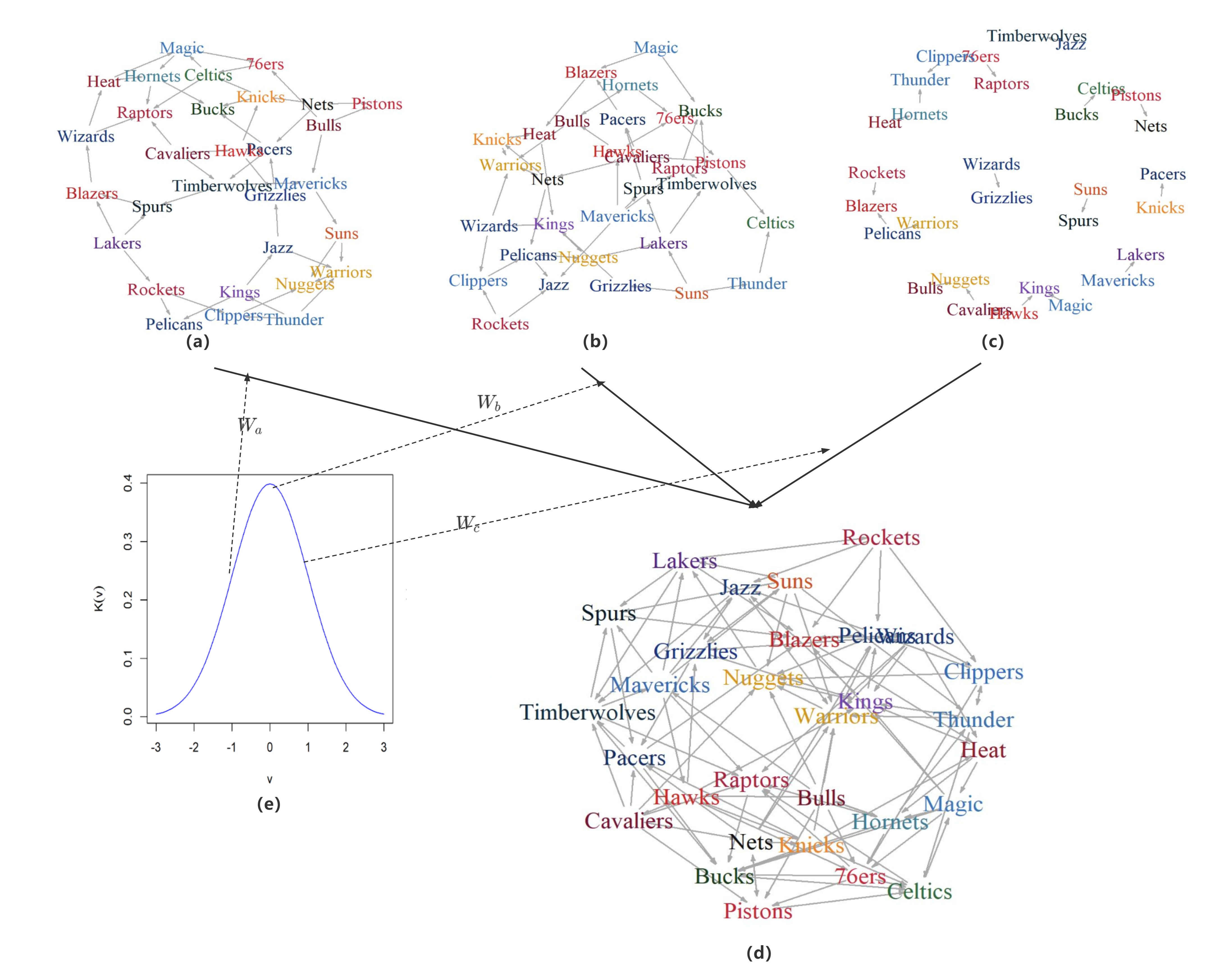
This section presents an NBA data example to demonstrate the advantages of the proposed dynamic method over the original static Rank Centrality methods of Negahban, Oh and Shah 2017 in Figure 1. In the NBA data example presented in Figure 1, sub-figures (a)–(c) show directed graphs generated by comparison results in three periods. The arrows in each graph represents the strength score transition from one node to another in the Markov chain. One common approach for treating dynamic ranking is to estimate the score vector independently for each graph, as adopted in the nearest neighbor frame (Karlé and Tyagi 2021). However, this method may not provide smoothly varying estimates and may suffer from insufficient comparisons for graph connectivity when the neighborhood is too narrow, such as a week of NBA game data can not ensure the connectivity. The proposed KRC method overcomes these issues by using a Gaussian kernel to generate time-dependent weights and aggregating (a)–(c) into a connected graph (d), ensuring the connectivity automatically. Compared to the static Rank Centrality method (Negahban, Oh and Shah 2017), the KRC method can estimate strength curves over a given period and has the advantage of exact online updating, which improves computation efficiency.
As pointed out by Negahban, Oh and Shah 2017 and Jain, Gilbert and Varma 2020, the computational cost of maximum likelihood estimation (MLE) for the Bradley-Terry model is much higher compared to Rank Centrality. In a dynamic setting, this computational issue becomes further complex in the presence of time-varying comparisons. However, an advantage of the proposed KRC method is the availability of exact online updating, which enables us to update (3.3) with a few matrix operations rather than optimization. Online updating significantly improves the computation efficiency of the method.
3.3 On-line Ranking
The proposed ranker (3.3) has an online version that updates the estimate as new observations for some pair come in. Specifically, we sequentially apply the Sherman–Morrison rank-one updating formula (Langville and Meyer 2006). This formula updates a stationary vector when a transition matrix perturbs only one row.
Lemma 1 (Rank-One Updating).
Let be a transition matrix. If the ith row of is updated to produce , the ith row of , and if and are the respective stationary vectors of and , then , where
| (3.4) |
is the group inverse of . Multiple row updates to requires applying this formula one row at a time and the group inverse must be sequentially updated. The updating formula for is as follows:
| (3.5) |
The updating formula mainly relies on the group inverse matrix, . The group inverse of a square matrix , which is a special case of the Drazin inverse, is the unique matrix satisfying , and . To perform updating, we define the rank-one updating operator by combining the updating formulas.
For the KRC updating, when a new observation for the pair arrives at time , the change only affects the -th and -th rows of the transition matrix. Let and denote the updated and old transition matrices, respectively. The perturbation vector for the -th row, , can be defined as:
| (3.6) |
Due to the construction of , the perturbation vector for the -th row, . Thus, we update the transition matrix in the -th and -th rows and then perform rank-one updating (Langville and Meyer 2006) twice to solve equation (3.3) online.
We present the detailed online updating method in Algorithm 2. This updating algorithm for the KRC method can be completed in just a few steps, avoiding the iterative optimization process in the MLE-based method.
4 Learning Theory
This section investigates various theoretical issues for the proposed ranker, including the uniqueness of (3.3), the rates of convergence, and most importantly, its asymptotic distribution.
The following conditions are assumed.
Assumption B (Capability ratios).
Assume that . Also, is three times continuously differentiable; .
Assumption B requires that the maximal discrepancy of the item’s skill score ratio is upper bounded and is sufficiently smooth as in Li and Racine 2007.
Assumption C (Kernel).
Kernel is nonnegative and symmetric, satisfying
Let .
Lemma 2 (Uniqueness).
Lemma 2 says that the solution of (3.3) is unique if there are abundant observations. Next we provide an error bound in terms of , , and .
The next theorem establishes the convergence rate for the KRC method.
Theorem 1 (Rates of convergence).
The first term is attributed to the variance of binary comparison, while the second term represents the bias due to the dynamic skill. Interestingly, the bias does not increase with an increased item number . Importantly, this error bound suggests that the optimal bandwidth is of order , which achieves the optimal trade-off between the bias and variance in that .
Next, we will present the asymptotic normality for the KRC method.
Theorem 2 (Finite-dimensional asymptotic normality).
The covariance matrix in the asymptotic normal distribution is diagonal, which means that the dependency from the comparisons between pairs is absent with the diverging . The independence between is consistent with the finding in the MLE of the static Bradley-Terry model (Simons and Yao 1999). The extra condition ensures that the remaining bias term, which is of high order , is much smaller than the variance term. The error analysis uses an inequality induced by the spectral norm of the error matrix defined by . For the error and the asymptotic distribution theory, we conduct entrywise analysis through a novel tool of the group-inverse matrix and its approximation. The group inverse is often involved in questions concerning Markov chains. Using an appropriate approximation technique, we give a sharp expansion for the Rank Centrality type estimator. The asymptotic normality and convergence rate are direct applications of this expansion. We will describe this novel tool and the expansion results in detail in the Appendix.
It is important to note that all the properties obtained for the spectral method when continue to hold without the condition . This condition, together with the assumption on , allows us to bound the bias term as the order . When there are not enough longitudinal observations but the error of is still guaranteed to be less than , the proof strategy still applies except that the size of the bias term increases. For example, when is a constant, which means we have a finite number of observations for in an interval with length , the bias term would increase to , but the variance part can still be analyzed using the same argumentation.
5 Simulations
This section presents simulation results to investigate the operating characteristics of the KRC method. In simulations, we simulate as follows:
- 1.
Generate from the uniform distribution U(1,3).
- 2.
For and , sample from U(0,1) and compute the capability parameter . Then generate the comparison result from .
In the first experiment, we increase from 10 to 100 by 10 to see the impact of the number of items on the performance while setting to see the effect of the sample size. For evaluation metric, we use the average normalized root mean squared error (RMSE), i.e. average error defined as and the max error defined as , based on 100 simulation replications. Moreover, we use the Gaussian kernel . And for the first experiment, we set the fixed bandwidth as .

As shown in Figure 2, the estimation error decreases as increases or increases. This observation is in accordant with the result of Theorem 1.
Concerning the bandwidth choice on the estimation of KRC, we draw the RMSEs under different bandwidths when and in Figure 3. As shown, the estimation error decreases initially, then increases, and eventually reaching equilibrium at the error of the Rank Centrality, as the bandwidth increases. The observation is consistent with the theoretical result of Theorem 1.
Next, we also compare KRC with the weighted maximum likelihood estimate (WMLE) of Bong et al. 2020 under various bandwidths in Figure 3, where WMLE is obtained by
| (5.1) |
In the experiment, we solve the nonlinearly constrained optimization with the MM algorithm for the Bradley-Terry model (Hunter 2004).

As demonstrated in Figure 3, the error achieved by our Kernel Rank Centrality method is nearly indistinguishable from that of WMLE. To further illustrate the advantage of the KRC method, we compared its computational efficiency with that of the WMLE under different problem sizes in Figure 4. Although the stationary distribution of the Markov chain can be computed using linear algebraic techniques, we used the power method in our experiment. The results show that the computational cost of the KRC method is significantly lower than that of the WMLE. Additionally, the advantage in computational efficiency becomes more pronounced as increases.

To illustrate the asymptotic distribution theory, we simulated the distribution of with and for this experiment. To reduce the bias, we used an under-smoothing approach (Chen 2017) with a smaller bandwidth . By comparing the empirical distribution of with its theoretical distribution defined in Section 4 in Figure 5, we see that the empirical density curve closely resembles the density of the normal distribution, which aligns with the marginal distribution according to the theory. To examine the diagonal elements of the covariance matrix, we included the correlation heatmap in Figure 6. The correlation coefficient of any pair is indeed close to zero, which is consistent with the asymptotic independence result suggested by Theorem 2.


6 Real Data Analysis
To test our model in practical settings, we consider dynamically estimating the abilities of National Basketball Association (NBA) teams over multiple seasons. We collected NBA data for ten regular seasons, from 2009-2010 to 2018-2019, from www.nba.com. During each NBA season, each team plays 82 regular games, resulting in 1230 regular season games. First, we test the forecasting performance of the Kernel Rank Centrality method using the following strategy:
- 1.
Encode the time of the -th game day in the -th season as , where is the size of the set of game days in the -th season.
- 2.
Take the games of the first seven seasons as the base and compute the team capability vector for each time point in the left three seasons with the data before .
- 3.
For each game in the left three seasons, we predict the winner of the game as the team with a larger skill score.
The proportion of correctly predicted matches, as the predictive accuracy, is used to measure performance. To determine whether the results produced by our model are reasonable, we compare our method with the relevant, openly available NBA Elo ratings (Silver and Fischer-Baum 2015). The Elo rating system is one of the most popular methods for estimating the competitors’ abilities in sports (Kovalchik 2020). The Elo rating is a dynamic system that updates the rating after each game. We compare the predicting performance of the Elo rating with our method under different bandwidths; see Table 1.
| 2016-2017 | 2017-2018 | 2018-2019 | Total | |
|---|---|---|---|---|
| RC | 0.6114 | 0.5732 | 0.5935 | 0.5927 |
| KRC(h=0.1) | 0.6228 | 0.6333 | 0.6341 | 0.6301 |
| KRC(h=0.5) | 0.6301 | 0.6317 | 0.6407 | 0.6341 |
| KRC(h=1) | 0.6455 | 0.6325 | 0.6366 | 0.6382 |
| KRC(h=1.5) | 0.6301 | 0.6081 | 0.6138 | 0.6173 |
| MLE | 0.6179 | 0.5740 | 0.5919 | 0.5946 |
| WMLE(h=0.1) | 0.6089 | 0.6260 | 0.6358 | 0.6236 |
| WMLE(h=0.5) | 0.6276 | 0.6260 | 0.6463 | 0.6333 |
| WMLE(h=1) | 0.6447 | 0.6236 | 0.6382 | 0.6355 |
| WMLE(h=1.5) | 0.6341 | 0.6065 | 0.6171 | 0.6192 |
| Elo | 0.6309 | 0.6325 | 0.6431 | 0.6355 |
Somewhat surprisingly, our method achieved comparable results to Elo and outperformed Elo when in the average accuracy. This result suggests that season-length data is more informative for estimation and prediction. Note that Elo is a feature-rich method that uses more feature data to adjust the margin of victory than KRC. We also present the performance of the static rank centrality, which had the worst results in all seasons. Our method can balance long-term strength and local features, leading to better performance in forecasting for the entire season.
Table 1 shows that the KRC method outperforms WMLE (Bong et al. 2020) for most bandwidths. While the MLE is the most commonly used method, it may not be effective in practice, where the Bradley-Terry or the dynamic Bradley-Terry assumption violates due to external covariates. Factors such as injuries, referees, and others may impact game results, causing them to deviate from the dynamic Bradley-Terry model. The results presented in Table 1 provide evidence that KRC is more suitable to such data than the MLE and its dynamic extensions.
We applied the KRC method to estimate the strength curve for each team. Figure 7 illustrates the changes in team strength over ten seasons. As shown, the Warriors and Spurs are the two standout teams during these seasons. The Warriors won three championships in the last five seasons, while the Spurs maintained a high level of strength throughout the ten seasons. The Lakers and Magic were top teams in the early seasons, but their strengths decreased rapidly. These results are consistent with reality, indicating that the curves estimated by our method can validly reflect changes in team strengths.

In addition to estimating team strength, one may also wish to construct a confidence interval for the winning probability between pairs of interest. Table 2 displays the estimated probability of one team winning over another at the end of the 2017-2018 season. The 95% confidence interval uses the distribution theory of and the delta method, with the bias term ignored in computation. Interestingly, the champion team of the season, the Warriors, outperformed others with a probability higher than 0.5. However, the 95% confidence interval with the Rockets team contains 0.5, suggesting that the Rockets were a strong opponent for the Warriors during the 2017-2018 season.
| Raptors | Nets | Warriors | Knicks | Pelicans | |
|---|---|---|---|---|---|
| Celtics | 0.57 | 0.25 | 0.61 | 0.18 | 0.37 |
| (0.51, 0.63) | (0.16, 0.33) | (0.55, 0.67) | (0.08, 0.28) | (0.30, 0.43) | |
| Mavericks | 0.77 | 0.45 | 0.80 | 0.35 | 0.59 |
| (0.68, 0.86) | (0.40, 0.51) | (0.70, 0.90) | (0.29, 0.42) | (0.51, 0.65) | |
| Rockets | 0.47 | 0.18 | 0.51 | 0.13 | 0.28 |
| (0.42, 0.53) | (0.08, 0.29) | (0.46, 0.57) | (0.01, 0.25) | (0.20, 0.37) | |
| Lakers | 0.76 | 0.44 | 0.78 | 0.34 | 0.58 |
| (0.67, 0.85) | (0.38, 0.49) | (0.69, 0.88) | (0.27, 0.41) | (0.52, 0.63) | |
| Pacers | 0.63 | 0.30 | 0.67 | 0.22 | 0.43 |
| (0.57, 0.70) | (0.22, 0.37) | (0.60, 0.74) | (0.13, 0.27) | (0.37, 0.48) | |
| Cavaliers | 0.75 | 0.43 | 0.78 | 0.33 | 0.57 |
| (0.66, 0.84) | (0.37, 0.49) | (0.68, 0.88) | (0.26, 0.40) | (0.51, 0.63) |
7 Discussion
This article introduces Kernel Rank Centrality (KRC), a spectral method devised to estimate item ratings in a dynamic setting based on the time-varying Bradley-Terry model. By integrating the Rank Centrality estimator with kernel smoothing techniques, KRC provides an accurate and efficient solution to the challenges posed by dynamic ranking. Our theoretical analysis of KRC demonstrates that its estimates converge to the dynamic Bradley-Terry model score with an error bound of . This paper also establishes the asymptotic normality of KRC’s distribution, a feat hitherto unachieved for spectral methods.
Our numerical investigation illuminates KRC’s efficacy in sports statistics and validates the developed theory, showcasing its computational efficiency. Data analysis using NBA statistics indicates that our ranking method outperforms the esteemed Elo method in forecasting accuracy, underscoring KRC’s effectiveness in dynamic rating. Thus, KRC can serve as a foundational tool for designing efficient algorithms for estimating and inferring sequential pairwise comparison data. Future research could explore time-dependent features and multi-dimensional comparison results to enhance KRC’s performance.
A Proofs of the results in Section 4
In this section, we begin by demonstrating the uniqueness result, followed by an analysis of the convergence rate. Then, we provide the expansion result for our KRC estimator. Furthermore, we leverage the expansion to establish the result and the Central Limit Theorem (CLT) as direct applications.
A.1 Proof of Lemma 2
The irreducibility of the chain is equivalent to the strong connectivity of the directed graph with the adjacency matrix . That means if we divide the items into two nonempty subsets, there exists some team in the first set and some team in the second set satisfy . Note that for , if has beat one time in the comparisons. Then a subset , the probability that is not connected with is less than . Let denote the event that is irreducible and . Note that and are constants. Then, when and are sufficiently large, we have
| (A.1) |
The last inequality holds with and .
A.2 Proof of the rate in Theorem 1
First we present the lemma of the perturbation bound for the leading left eigenvector of the probability transition matrix, a result developed in Negahban, Oh and Shah 2017 and Chen et al. 2019.
Lemma 3.
For two reversible Markov chains defined with transition matrix and . Suppose the stationary distributions are and respectively. Let and be the max absolute eigenvalue except . If , then
By virtue of Lemma 3, the perturbation of the stationary distribution of the designed reversible Markov chain is dictated by two important quantities: (i) the condition number and (ii) the noise size . The first part is controlled by the following lemma, which is a direct result induced from the proposition in static Rank Centrality (Negahban, Oh and Shah 2017).
Lemma 4.
If and is the transition matrix defined in (3.2), we have
For the left part, we will show the noise size is well bounded by our kernel method with some mild conditions. For , let , and denote , and , respectively.
Lemma 5.
Under the conditions in Theorem 1, there exists global constants and , such that
Proof of Lemma 5:
It is noted that the error matrix can be decomposed as where the superscript , and denote the diagonal matrix, upper triangular matrix, and lower triangular matrix, respectively. Then we deal with these three terms separately. By the definition of the spectral norm, we know
| (A.2) |
where,
and
is a sum of bounded independent random variables. Using Hoeffding’s inequality, we have
When is large enough, we have
Let and we have that
| (A.3) |
Then we move on to , which is the fluctuation part caused by the dynamic strength. As and ,
| (A.4) |
Let . We get, when is sufficiently small,
Hence, together with (A.3), we complete the bound for ,
| (A.5) |
For the upper triangular part , we apply the similar decomposition, where and are upper triangular matrices defined by and With the result of , we have To deal with , we decompose it as a sum of independent random matrices, is an matrix whose elements are zeros except . Then we can bound these independent matrices by,
| (A.6) |
The second inequality holds with the fact that when is sufficiently large. Note that the elements in are independent. We also have
Then applying the matrix Bernstein’s inequality (Tropp 2012), it holds that for any ,
Let and combining . Then
| (A.7) |
The similar arguments lead to the same upper bound for , which we omit for brevity. Finally, let and we complete the proof by combining the constant multipliers in these bounds.
Proof of rate in Theorem 1:
By the bounds of and , we have that holds with probability at least , when is sufficiently small. Then we only need to demonstrate the bound to complete the proof of rate in Theorem 1. For simplicity of discussion, we decompose into and . With the discussion in the proof of Lemma 5, we know with a global constant. As a result,
| (A.8) |
So we focus on . Note that is constructed by . Then is in a quadratic form of , the dimensional column vector from . Specifically,
where is an matrix. For convenience, we use the subscript denote the row or column corresponding to . The matrix is defined by
| (A.9) |
Then is a weighted Laplacian matrix with and . Then by the spectrum theory of Laplacian matrices (Mohar 1991), we can obtain
Hence, . And the Frobenius norm of can be bounded by
Note that is subgaussian. Then by Hanson-Wright inequality (Rudelson and Vershynin 2013), we can derive, for some constant ,
| (A.10) |
A.3 Expansion results for the spectral method
We first present a non-asymptotic expansion for the KRC method, which is a direct result from the Maclaurin expansion for an irreducible Markov chain (Cao 1998).
Lemma 6 (Maclaurin expansion).
Let and denote the group inverse of . If , then
| (A.12) |
To analyze the asymptotics of as , we need to know the structure of . One way is to approximate by in a simple form such that
To achieve this, we observe that the group inverse matrix can be approximated by a diagonal matrix with the max column error bounded by .
Theorem 3 (Group inverse approximation).
Let be a diagonal matrix with the diagonal elements defined by
Then when , we have,
The approximation is in a sharp and simple form such that the asymptotic property is easy to analyze. With this approximation, we simplify the expansion in (A.12) in a more concise and tractable form.
Next, we express the entrywise expansion as a sum of these pairwise error terms.
Theorem 4 (Entrywise expansion).
Under the assumptions of Theorem 1, for any and , if , and , we have, with probability tending to ,
where and .
The proof of this expansion involves substituting into (A.12) and bounding the remaining terms. A similar expansion result is also derived for the static setting in recent work by Gao, Shen and Zhang 2023. However, their proof relies on a result of convergence rate (Chen et al. 2019) and the leave-one-out trick. For our method, the convergence rate is a direct consequence of this expansion, making our approach more straightforward. Using this expansion, we can easily derive the convergence rate and the finite-dimensional asymptotic normality for the in the previous subsection.
Proof of Theorem 3:
By the property of the Markov chain and the group inverse, we have Then for ,
| (A.13) |
In the right side, by direct calculations, it is shown that
| (A.14) | ||||
Let . Combine these parts and we have and for ,
Note that and are when is . Hence . For the left side,
| (A.15) |
where is the minimum singular value of . It is noted that when is . With the result of Lemma 4, we obtain that Together with , we get that is .
Proof of Theorem 4:
When , for any ,
By the discussion in the proof of Theorem 1, the condition holds with probability tending to one. The first term is the main term in the expansion. For simplicity, we omit the notation of time when there is no ambiguity. Plugging the approximation in the first term of the expansion, we derive the entrywise expansion for . For ,
| (A.16) |
We denote the three parts in right side of the expansion as , and . is tractable due to the simple form of ,
| (A.17) |
Using Hoeffding’s inequality and the similar technique in bounding , we see that is . Then we need to prove that the remaining parts are . Note that each element of is bounded and we have
| (A.18) |
Then use the decomposition again,
| (A.19) |
For , we have
| (A.20) |
The last inequality is obtained with the bound in (A.3). By Hoeffding’s inequality, we can derive that is . For the bias term ,
| (A.21) |
The first inequality follows from Cauchy-Schwartz’s inequality and the fact that the bias for each element is . Combining the bound of and the bound of the bias term in , we can obtain that .
is the second order remainder. To handle this term, we decouple the dependence of and by replacing with ,
By Theorem 1, is and is . Then by the norm property,
| (A.22) |
Note that when . Then, .
For , we substitute the decomposition of ,
| (A.23) |
Denote the four parts as , , and , respectively, where is tractable for analysis. We can analyze the norm for the multiplicative product step by step. Let be the diagonal matrix of . With the facts and , we have For each ,
| (A.24) |
Decompose again and we have
| (A.25) |
We decompose again in the last step,
| (A.26) |
When , is . These steps will be helpful when we bound and . For , from the previous result, we know . So use the same decomposition method in (A.25) and (A.26), and we derive that . Note that . We can derive the bound for in the same manner as analyzing . Hence, we also have . When and , . So we have and are both . Then for , it can be written as the quadratic form of ,
| (A.27) |
where is an matrix and is an matrix. Next we will present the bounds for the spectral norm and Frobenius norm of . It is noted that is the same matrix defined in (A.9) and . The discussion for is similar with that of . has the same structure with . By replacing with , we have So the order for is . Combine the two bounds and we can control the spectral norm of by
| (A.28) |
For simplicity, we denote by . To handle the Frobenius norm, we derive the explicit form of . In fact, is the second derivative matrix of with respect to . For the pairs and , the second order derivative is in the following form,
| (A.29) |
So we can bound the Frobenius norm by
| (A.30) |
Then we discuss the expectation of .
The last inequality is from the facts that and Then by the Hanson-Wright inequality (Rudelson and Vershynin 2013), we can derive that is . Finally, combine the bounds for , , , and we prove that is .
A.4 Proof of Theorem 2
By the expansion, we have for any , with probability tending to 1,
Let denote the event that the expansion holds true. We first show the conditional asymptotic normality under . Let denote the main term in the expansion. It suffices to prove that for any fixed and , Note that
and
Then
| (A.31) |
It is noted that each term in the second term is . Hence,
Moreover, the Lindeberg-Feller condition holds trivially since are bounded. So by Lindeberg-Feller Central Limit Theorem, . The proof is complete with the fact that for every ,
References
- Bong et al. (2020) Bong, H., Li, W., Shrotriya, S. and Rinaldo, A. (2020). Nonparametric estimation in the dynamic Bradley-Terry model. In International Conference on Artificial Intelligence and Statistics 3317–3326. PMLR.
- Bradley and Terry (1952) [author] Bradley, Ralph AllanR. A. and Terry, Milton E.M. E. (1952). Rank Analysis of Incomplete Block Designs: I. The Method of Paired Comparisons. Biometrika 39 324–345. 10.2307/2334029
- Brémaud (2013) [author] Brémaud, PierreP. (2013). Markov chains: Gibbs fields, Monte Carlo simulation, and queues 31. Springer Science & Business Media.
- Cao (1998) [author] Cao, Xi-RenX.-R. (1998). The Maclaurin series for performance functions of Markov chains. Advances in Applied Probability 30 676–692. 10.1239/aap/1035228123
- Cattelan, Varin and Firth (2013) [author] Cattelan, ManuelaM., Varin, CristianoC. and Firth, DavidD. (2013). Dynamic Bradley–Terry modelling of sports tournaments. Journal of the Royal Statistical Society: Series C (Applied Statistics) 62 135-150. 10.1111/j.1467-9876.2012.01046.x
- Chen (2017) [author] Chen, Yen-ChiY.-C. (2017). A tutorial on kernel density estimation and recent advances. Biostatistics & Epidemiology 1 161-187. 10.1080/24709360.2017.1396742
- Chen et al. (2019) [author] Chen, YuxinY., Fan, JianqingJ., Ma, CongC. and Wang, KaizhengK. (2019). Spectral method and regularized MLE are both optimal for top- ranking. The Annals of Statistics 47 2204 – 2235. 10.1214/18-AOS1745
- Fahrmeir and Tutz (1994) [author] Fahrmeir, LudwigL. and Tutz, GerhardG. (1994). Dynamic Stochastic Models for Time-Dependent Ordered Paired Comparison Systems. Journal of the American Statistical Association 89 1438-1449. 10.1080/01621459.1994.10476882
- Gao, Shen and Zhang (2023) [author] Gao, ChaoC., Shen, YandiY. and Zhang, Anderson YA. Y. (2023). Uncertainty quantification in the Bradley–Terry–Luce model. Information and Inference: A Journal of the IMA 12 1073-1140. 10.1093/imaiai/iaac032
- Gleich (2015) [author] Gleich, David F.D. F. (2015). PageRank Beyond the Web. SIAM Review 57 321-363. 10.1137/140976649
- Glickman (1999) [author] Glickman, Mark E.M. E. (1999). Parameter Estimation in Large Dynamic Paired Comparison Experiments. Journal of the Royal Statistical Society: Series C (Applied Statistics) 48 377-394. https://doi.org/10.1111/1467-9876.00159
- Glickman (2001) [author] Glickman, Mark E.M. E. (2001). Dynamic paired comparison models with stochastic variances. Journal of Applied Statistics 28 673-689. 10.1080/02664760120059219
- Han et al. (2020) [author] Han, RuijianR., Ye, RougangR., Tan, ChunxiC. and Chen, KaniK. (2020). Asymptotic theory of sparse Bradley–Terry model. The Annals of Applied Probability 30 2491 – 2515. 10.1214/20-AAP1564
- Hunter (2004) [author] Hunter, David R.D. R. (2004). MM algorithms for generalized Bradley-Terry models. The Annals of Statistics 32 384 – 406. 10.1214/aos/1079120141
- Jain, Gilbert and Varma (2020) Jain, L., Gilbert, A. and Varma, U. (2020). Spectral Methods for Ranking with Scarce Data. In Proceedings of the 36th Conference on Uncertainty in Artificial Intelligence (UAI) (J. Peters and D. Sontag, eds.). Proceedings of Machine Learning Research 124 609–618. PMLR.
- Karlé and Tyagi (2021) [author] Karlé, EglantineE. and Tyagi, HemantH. (2021). Dynamic Ranking with the BTL Model: A Nearest Neighbor based Rank Centrality Method. arXiv preprint arXiv:2109.13743.
- Kovalchik (2020) [author] Kovalchik, StephanieS. (2020). Extension of the Elo rating system to margin of victory. International Journal of Forecasting 36 1329-1341. 10.1016/j.ijforecast.2020.01.006
- Langville and Meyer (2006) [author] Langville, Amy N.A. N. and Meyer, Carl D.C. D. (2006). Updating Markov Chains with an Eye on Google’s PageRank. SIAM Journal on Matrix Analysis and Applications 27 968-987. 10.1137/040619028
- Langville and Meyer (2012) [author] Langville, Amy NA. N. and Meyer, Carl DC. D. (2012). Who’s# 1?: the science of rating and ranking. Princeton University Press.
- Li and Racine (2007) [author] Li, QiQ. and Racine, Jeffrey ScottJ. S. (2007). Nonparametric econometrics: theory and practice. Princeton University Press.
- Liu, Fang and Lu (2022) [author] Liu, YueY., Fang, Ethan XE. X. and Lu, JunweiJ. (2022). Lagrangian inference for ranking problems. Operations Research.
- Liu et al. (2019) [author] Liu, QinghuaQ., Crispino, MartaM., Scheel, IdaI., Vitelli, ValeriaV. and Frigessi, ArnoldoA. (2019). Model-Based Learning from Preference Data. Annual Review of Statistics and Its Application 6 329-354. 10.1146/annurev-statistics-031017-100213
- Maystre, Kristof and Grossglauser (2019) Maystre, L., Kristof, V. and Grossglauser, M. (2019). Pairwise Comparisons with Flexible Time-Dynamics. In Proceedings of the 25th ACM SIGKDD International Conference on Knowledge Discovery & Data Mining. KDD ’19 1236–1246. Association for Computing Machinery, New York, NY, USA. 10.1145/3292500.3330831
- Mazzuchi, Linzey and Bruning (2008) [author] Mazzuchi, Thomas A.T. A., Linzey, William G.W. G. and Bruning, ArminA. (2008). A paired comparison experiment for gathering expert judgment for an aircraft wiring risk assessment. Reliability Engineering & System Safety 93 722-731. 10.1016/j.ress.2007.03.011
- McHale and Morton (2011) [author] McHale, IanI. and Morton, AlexA. (2011). A Bradley-Terry type model for forecasting tennis match results. International Journal of Forecasting 27 619-630. 10.1016/j.ijforecast.2010.04.004
- Mohar (1991) Mohar, B. (1991). The Laplacian spectrum of graphs. In Graph Theory, Combinatorics, and Applications (Y. Alavi, G. Chartrand, O. Oellermann and A. Schwenk, eds.) 2 871 – 898. Wiley.
- Negahban, Oh and Shah (2017) [author] Negahban, SahandS., Oh, SewoongS. and Shah, DevavratD. (2017). Rank Centrality: Ranking from Pairwise Comparisons. Operations Research 65 266-287. 10.1287/opre.2016.1534
- Rudelson and Vershynin (2013) [author] Rudelson, MarkM. and Vershynin, RomanR. (2013). Hanson-Wright inequality and sub-gaussian concentration. Electronic Communications in Probability 18 1 – 9. 10.1214/ECP.v18-2865
- Shah and Wainwright (2018) [author] Shah, Nihar B.N. B. and Wainwright, Martin J.M. J. (2018). Simple, Robust and Optimal Ranking from Pairwise Comparisons. Journal of Machine Learning Research 18 1-38.
- Silver and Fischer-Baum (2015) [author] Silver, NateN. and Fischer-Baum, ReubenR. (2015). How we calculate NBA Elo ratings. http://fivethirtyeight. com/features/how-we-calculate-nba-elo-ratings.
- Simons and Yao (1999) [author] Simons, GordonG. and Yao, Yi-ChingY.-C. (1999). Asymptotics when the number of parameters tends to infinity in the Bradley-Terry model for paired comparisons. The Annals of Statistics 27 1041 – 1060. 10.1214/aos/1018031267
- Tropp (2012) [author] Tropp, Joel AJ. A. (2012). User-friendly tail bounds for sums of random matrices. Foundations of computational mathematics 12 389–434. 10.1007/s10208-011-9099-z
- Vaziri et al. (2018) [author] Vaziri, BabackB., Dabadghao, ShaunakS., Yih, YuehwernY. and Morin, Thomas L.T. L. (2018). Properties of sports ranking methods. Journal of the Operational Research Society 69 776-787. 10.1057/s41274-017-0266-8
- Zhou et al. (2019) [author] Zhou, WangW., Li, JianpingJ., Zhou, YongluanY. and Memon, Muhammad HammadM. H. (2019). Bayesian pairwise learning to rank via one-class collaborative filtering. Neurocomputing 367 176-187. 10.1016/j.neucom.2019.08.027