The Weyl-Wigner representation of quantum mechanics allows one to map the density operator in a function in phase space — the Wigner function — which acts like a probability distribution. In the context of statistical mechanics, this mapping makes the transition from the classical to the quantum regimes very clear, because the thermal Wigner function tends to the Boltzmann distribution in the high temperature limit. We approximate this quantum phase space representation of the canonical density operator for general temperatures in terms of classical trajectories, which are obtained through a Wick rotation of the semiclassical approximation for the Weyl propagator. A numerical scheme which allows us to apply the approximation for a broad class of systems is also developed. The approximation is assessed by testing it against systems with one and two degrees of freedom, which shows that, for a considerable range of parameters, the thermodynamic averages are well reproduced.
Semiclassical approximation of the Wigner function for the canonical ensemble
keywords
Weyl-Wigner representation, canonical ensemble, semiclassical approximations, Kerr system, Morse potential, Nelson potential1 Introduction
Quantum and classical statistical mechanics differ both in their formulation and in their results. It is not by chance that the first evidence for quantum mechanics is the black-body spectrum derived by Planck Planck 1901. The canonical ensemble, which describes a system in equilibrium with a thermal bath of temperature , is characterized classically through a probability distribution over phase space, the Boltzmann distribution
| (1) |
where, is a point in the phase space spanned by the coordinates and the momenta , is the classical Hamiltonian of the system, is the classical partition function and , being the Boltzmann’s constant. The quantum canonical ensemble, on the order hand, is described by the thermal density operator
| (2) |
where is the Hamiltonian operator and is the quantum partition function. Both (1) and (2) allow one to calculate thermodynamic averages, and although the results agree for high temperatures, there is a considerable discrepancy for low ones. With the introduction, by Wigner, of his eponymous function Wigner 1932, the differences between these two formulations diminished, as it allows one to map the thermal density operator in a function over phase space that works as if it were a probability distribution, though it strongly deviates from (1) in the low temperature regime. This proposal further evolved to give a complete formulation of quantum mechanics in phase space Groenewold 1946; Moyal 1949, which we call the Weyl-Wigner representation. The high temperature limit of the resulting semiclassical approximation of the thermal Wigner function, coincides with the classical distribution (1).
A further advantage of the Weyl-Wigner formalism is that common observables with classical correspondence are directly represented by the classical phase space function, or a function that is semiclassically close to it. Thus, there is no limitation to Hamiltonians with a quadratic momentum dependence: any real phase space function will do. Moreover, the expectation of the observable is evaluated by a phase space integral, identical to its classical counterpart, except that the Liouville distribution is replaced by the Wigner function. In contrast, the phase space reflection operator,
| (3) |
which corresponds classically to the canonical reflection through a phase space point, is also a quantum observable. Indeed, this displaced parity operator has real eigenvalues , which makes it as quantum an observable as a spin. The essential role that this operator plays in the Wigner-Weyl representation, uncovered by Grossmann Grossmann 1976 and Royer Royer 1977 identifies its expectation with the Wigner function itself:
| (4) |
In short, the value of the Wigner function at every point in phase space supplies the expectation of the reflection operator for that point, which is exactly how it has been verified experimentally Bertet et al. 2002, by counting even and odd outcomes of phase space reflections on identically prepared states.
In this paper, we will explore the fact that, by evaluating a propagator at an imaginary time , where is the thermal time, we obtain the operator , which is proportional to the thermal density operator (2). This is the so called Wick rotation Ingold 2002; Greiner et al. 2013. We will employ this relation, together with a semiclassical approximation for the propagator, which expresses it in terms of classical trajectories, to obtain a semiclassical approximation for the canonical ensemble. In principle, it provides a powerful method for evaluating the thermal density operator at lower temperatures, even for many degrees of freedom, because classical trajectories are computed in parallel. The present initial exploration is limited to two degrees of freedom.
The complexification of the Hamiltonian to adapt it to a thermal, rather than a real evolution is already well established in semiclassical calculations, mainly within the chemical literature Yan et al. 2019; Zhao and Miller 2002; Shao and Pollak 2006; Liu and Miller 2006; Pollak and Martin-Fierro 2007; Liu and Miller 2011a; Liu and Miller 2011b and De Carvalho et al. 1999; de Carvalho et al. 2000. Even though the various alternative propagators are also supported by trajectories in phase space, the end result is the position density matrix. Then a comparison with the classical distribution depends on Wigner’s symmetrized Fourier transform over phase space. Furthermore, the complexification is confined to the momentum, which restricts the Hamiltonian to be the sum of a quadratic kinetic term with a potential energy, which excludes even a simple magnetic field. In contrast, the complexification employed here is, of need, much less simple (even in the case of the quadratic momentum dependence favoured by the position representation), so as to accommodate arbitrary Hamiltonians, for which the real time evolution is inaccessible to the differential Schrödinger equation. Thus, together with computational tests for standard Hamiltonians, we test the thermal averages of Birkhoff normal forms Arnol’d et al. 2013; De Almeida 1988, which include the quartic Kerr Hamiltonian Haroche and Raimond 2006; in its turn, the unit cell of the many-body Bose-Hubbard Hamiltonian Schlagheck et al. 2019.
This paper is a followup on Ozorio de Almeida et al. 2021, where the core results of our current approach were first proposed. Here, we bridge the gaps that remained, which then allows us to devise a computational scheme that opens the possibility of applying our approximation to a vast number of cases. These new developments were achieved during a master’s degree, and first appeared on the thesis Gil de Oliveira 2023.
The presentation is then structured as follows: in section 2 we discuss elements of the Weyl-Wigner representation and introduce a semiclassical approximation for the propagator. In section 3 we particularize this discussion for the canonical ensemble, and show how the approximation for the propagator generates an approximation for the thermal density operator through the Wick rotation. In section 4, we apply our approximations for normal forms, which are a class of systems for which one has explicit expressions for the required quantities. In section 5 we reformulate the calculation of the trajectories in terms of a duplicated phase space, which is more amenable to a computational treatment, and develop a complete numerical method that allows us, in principle, to apply our approximation for systems with an arbitrary hamiltonian. In sections 6 and 7, we use this numerical scheme to apply the approximation to the Morse system, which has one degree of freedom, and to the Nelson system, which has two.
2 The Weyl-Wigner representation and semiclassical approximations
The Weyl-Wigner representation of quantum mechanics is based on the reflection operators
| (5) |
which corresponds classically to the transformation . Here, is a vector formed by the position and momentum operators and denotes the wedge product, defined by , with
| (6) |
where denotes the identity matrix.
The Wigner symbol of an operator is then given by
| (7) |
Furthermore, the Wigner function is a quantity proportional to the Wigner symbol of the density operator
| (8) |
and can be used to calculate quantum averages
| (9) |
as if it were a probability distribution.
As an example, we observe that the Wigner function for the eigenstates of the harmonic oscillator, defined by a hamiltonian , are given by
| (10) |
where is the th Laguerre polynomial Groenewold 1946.
A striking feature of the Wigner representation is the fact that the Wigner symbol of operators of the form is simply , which is exactly the corresponding classical variable. This is not a general result, as there can be corrections in form of power series of . A useful formula for calculating more complicated Wigner symbols is the Groenewold rule Ozorio de Almeida 1998
| (11) | ||||
The Wigner symbol of the propagator
| (12) |
is called the Weyl propagator, and, for short enough times, has the semiclassical approximation Ozorio de Almeida 1998
| (13) |
Here, is the so called (centre) action, and
| (14) |
is proportional to its hessian. The action has the role of a generating function for the classical hamiltonian flow. It indirectly specifies the transformation by giving the chord
| (15) |
in terms of the centre
| (16) |
through the relation
| (17) |
As going back in time simply reverses the hamiltonian flow, we must have , from which we conclude that the centre action must be an odd function of . Furthermore, Hamilton’s equations
| (18) |
imply that, for short times , we have
| (19) |
from which we get
| (20) |
In general, the action is given by
| (21) |
where is the symplectic area of the region between the trajectory and the chord and is the energy of the trajectory.
As an example for quadratic hamiltonians
| (22) |
the action is also quadratic and given by
| (23) |
It is important to observe that, for this class of systems, the semiclassical approximations are actually exact Ozorio de Almeida 1998. For a harmonic oscillator with frequency , we have , and we obtain an exact Weyl propagator
| (24) |
We see that, when , we have
| (25) |
The set of points where this divergence occurs is called a caustic, and it signals the breakdown of the description of the canonical transformation by the centre generating function. For the harmonic oscillator, the hamiltonian flow in these instants is simply a reflection , and therefore, for every pair we get the same centre . In this case, then, the caustics are the entire phase space, but, for non quadratic hamiltonians, these divergences may be restricted to a lower dimensional sub-manifold. In general, after crossing a caustic, there may be more than one chord for each centre, and the approximation for the propagator becomes a sum of terms like (13), where one must include an extra Maslov phase in the exponents Ozorio de Almeida and Ingold 2014; Nicacio et al. 2017.
It is possible to show Ozorio de Almeida 1998 that the jacobian
| (26) |
of the hamiltoninan flow, which is a symplectic matrix Arnol’d 2013, is related to through the Cayley parametrization Arnol’d et al. 2013
| (27) |
allowing us to rewrite (13) as
| (28) |
which will be the most convenient form of the semiclassical propagator to work with.
3 The canonical ensemble in phase space
As mentioned in the introduction, this work is based on the evaluation of the semiclassical approximation for the propagator (28), at the imaginary time , being the thermal time. We then obtain a semiclassical approximation for :
| (29) |
where we have defined the euclidean action , which is necessarily real, as is an odd function of . For the harmonic oscillator, we get, using (24),
| (30) |
It is interesting to note that, by using the the short time approximation (20) and setting , we get
| (31) |
that is, for high temperatures, we recover the classical canonical ensemble.
In this framework, the thermodynamic expectation values
| (32) |
are completely determined if one is able to calculate expressions of the form for imaginary , which has an approximation
| (33) |
One of the first problems that appears when dealing with semiclassical approximations, and can already be seen in (33), is the fact that the relevant trajectories are specified by boundary-conditions — in the case of the Wigner representation, we specify the centre defined by the endpoints of the trajectory — that can be satisfied by more than one orbit, and are much more difficult to solve than an initial value problem. This is the so called root search problem.
There are a few methods that can be used to circumvent this question, including the Initial and Final Value Representations Ozorio de Almeida et al. 2013. Here, we briefly discuss a method that is specially adapted for he calculation of (33), which we call the midpoint representation, and consists of a mere change of variables, that we explain in what follows. We start with a point in phase space — the midpoint — from which we propagate a trajectory , that evolves forward in time, and a trajectory , which evolves backwards, as illustrated in figure 1.
In other words, satisfy the pair of initial value problems
| (34) |
From this trajectory, we construct a centre
| (35) |
and a chord
| (36) |
Then, the transformation has a jacobian determinant
| (37) | ||||
where we have used the fact that symplectic matrices, such as , have unit determinant, and that the composition law holds. Performing this change of variables in (33), we arrive at
| (38) |
Furthermore, in this framework, the area can be explicitly calculated as Ozorio de Almeida et al. 2021
| (39) |
from which we obtain the action
| (40) |
4 Normal Forms
Here, we discuss a class of systems for which we are able to obtain explicit analytical results for the trajectories (34), which allow a direct evaluation of (38) at imaginary times.
A one dimensional classical hamiltonian written as
| (41) | ||||
is said to be in Birkhoff normal form Arnol’d et al. 2013; De Almeida 1988. Its orbits are circles in phase space, and, therefore, by a simple geometric argument, one may find explicit expressions for all the ingredients of the semiclassical approximation, as done in Ozorio de Almeida et al. 2021. Defining the action variable
| (42) |
and
| (43) |
we find the euclidean action
| (44) |
the centre
| (45) |
and the jacobian determinant
| (46) | ||||
Quantum hamiltonians that can be written as
| (47) |
have a Wigner symbol that is a Birkhoff’s normal form, but, except in the case of the harmonic oscillator, the function in (41) does not coincide with . Formulas for the calculation of the symbols are presented in 9.
Some of the quantum properties of this class of systems are also readily obtained — they share their eigenstates with the harmonic oscillator, and for a quantum normal form described by a hamiltonian , the eigenenergies are simply . This simplicity makes the comparison of our semiclassical approximation with the quantum result straightforward.
It is instructive to analyze the behaviour of our approximation in the low temperature limit. By squaring (45), we obtain
| (48) |
Interpreting this equation as an implicit definition of , we see that, for a fixed , in order for the right side of the equality to remain finite, we must have
| (49) |
Therefore, for systems that satisfy , we see that, according to (48), has the asymptotic behaviour
| (50) |
Substituting this expression in (44) and taking the limit , we obtain, except for a constant term in ,
| (51) |
and the semiclassical approximation converges to the quantum result, that is, the semiclassical approximation for the thermal Wigner function tends to the Wigner function of the ground state of the harmonic oscillator, given in (10). Therefore, we see that, at least for normal forms with , the semiclassical approximation is well anchored in both the high temperature limit, as it coincides with the classical result, and in the low temperature one, as it correctly predicts the ground state. It then remains to analyze its behaviour for intermediate temperatures.
4.1 Kerr system
The simplest case, beyond the harmonic oscillator, of a system governed by a normal form is probably the Kerr system, whose Hamiltonian is
| (52) |
where is a dimensionless parameter and is a frequency. This Hamiltonian models the propagation of light through a medium with cubic electric susceptibility Haroche and Raimond 2006. The time evolution of coherent states under its action is known Yurke and Stoler 1986; Averbukh and Perelman 1989, and the corresponding Wigner function has been experimentally measured Kirchmair et al. 2013. This evolution has also been successfully simulated, in the case with , utilizing semiclassical techniques Lando et al. 2019. A further point of interest is that the Hamiltonian for the Bose-Hubbard chain Schlagheck et al. 2019 in many-body physics can be considered as a coupling of Kerr oscillators, which highlights the importance of exploring semiclassical methods for Hamiltonians with non-quadratic momenta.
We note that, in this case, the Wigner symbol of the Hamiltonian only coincides with its classical counterpart within a constant term, as, with the aid of (11), one finds
| (53) |
Identifying
| (54) |
we see that
| (55) |
and, therefore, we should expect a good result for low temperatures. Furthermore, when , we also expect a good result, as, when , we recover the harmonic oscillator, for which the semiclassical approximation is exact. We also note that, because
| (56) |
one sees that , that is, there are no caustics for imaginary time.
In figure 2, we show the expectation value of the energy as a function of thermal time for different values of the parameter .
In the canonical ensemble, the specific heat can be calculated in terms of the variance in the energy:
| (57) |
In this case, the Wigner symbol of the square of the hamiltonian is significantly different from . With this is mind, we show, in figure 3, the specific heat as a function of thermal time for different values of .
As one sees, the quality of our semiclassical approximation is heavily dependent on the parameter . As increases, we see a deviation from the quantum results for intermediate values of , although, as foreseen, we have a good agreement at both high and low temperatures.
It may seem somewhat disturbing that the semiclassical approximation does not respect the positivity of the heat capacity: the figure cuts off the negative region. Yet it must be recalled that errors in and may be added, whereas the averages are subtracted. Indeed, Fig. 4 shows that the variance in (57) is considerably smaller than . In general one may then expect the heat capacity to be a much more stringent test of approximations than the energy average, as will occur further in our examples. One should note that a semiclassical version of the heat capacity as a second derivative of the partition function is not viable, as discussed in Ozorio de Almeida et al. 2021.
5 Double Phase Space
If we wish to apply our approximation for a broader class of systems, we must resort to numerical techniques. In this section, we restate the calculation of the terms in the integrand (38) in a way that is well adapted for a numerical solution, and, in the following sections, we apply this method for a few more systems.
Instead of obtaining the centre in equation (16) propagating two trajectories, one forward and one backwards in time, it will be easier to calculate a single forward trajectory in a double phase space. In this new space, the centre will play the role of position, while the conjugate momentum is given by . The double hamiltonian de Almeida et al. 2009; Brodier and de Almeida 2010; Koda 2015
| (58) | ||||
will then give the correct equations of motion, as one may check:
| (59a) | ||||
| (59b) | ||||
For a given midpoint , these equations must then be solved under the initial conditions
| (60) |
In order to be able to define the trajectories for complex times, we simply promote the derivatives with respect to in (59) to derivatives with respect to a complex number :
| (61) | ||||
If the functions and defined by these equations turn out to be analytic, then the line integral
| (62) |
which would be the extension of the area , given in (39), for the complex plane, is only dependent on the endpoints of the path , which are and .
Assuming this is the case, we choose to be the easiest path that joins and — the line segment — and parameterise it by the arc-length . The explicit expression for the parametrization is then
where . This path is illustrated in figure 5.
Now, we compose and with , that is, we define the functions and . By the chain rule, we deduce that these functions satisfy
| (63) |
which are almost Hamilton’s equations with real time . If we define , where ∗ denotes complex conjugation, and the modified hamiltonian
| (64) | ||||
we, in fact, recover proper Hamilton’s equations
| (65) | ||||
although with a hamiltonian that is generally complex, but that reduces to a real function if , which is the case for our interests ().
In terms of these quantities, the area is given by
| (66) |
which, alternatively, may be cast in the form of a initial value problem
| (67) | ||||
The last missing ingredient is a way to calculate the jacobian . It can be obtained by differentiating (65) with respect to , which give us the equations
| (68a) | |||
| (68b) |
solved under the initial conditions
| (69) |
In order to calculate (38) with , one must then solve the initial value problems specified by (65), (67) and (68) with , and obtain the solution at . If we have degrees of freedom, this will be a system of coupled differential equations with real variables. For the remaining of this work, we will test the procedure here described for the cases .
It should be noted that the definition of a real double Hamiltonian in replacement of a complex Hamiltonian is not unique. Our construction, specially suited to the Wigner-Weyl representation, coincides neither with the double Hamiltonians designed for propagating coherent states by de Aguiar et al. De Aguiar et al. 2005, nor with the double Hamiltonian for the Boltzmann operator of Yan and Shao Yan et al. 2019. Indeed, the double trajectories in this reference decouple into pairs of simple trajectories, due to the assumption of a quadratic momentum dependence.
For each choice of decomplexification one obtains different trajectories in their own phase space. Unlike the simple equivalence of the various variants related directly by Fourier transforms, the SC equivalence for decomplexified Hamiltonians is, so far, a question which relies on numerical investigaton. A mixed position-momentum representation is employed in Yan et al. 2019 to derive their semiclassical approximation of the density matrix, but it requires a further Fourier transform (beyond the Wigner transform) to relate their phase space formulae to the thermal Wigner function. It is interesting that a composition of Herman-Kluck propagators evolving for positive and negative half-times is also proposed, but there it is only optional, in contrast to its essential role within the present more general theory,
6 Morse System
The Morse potential Morse 1929 is given by the expression
| (70) |
where is a radial coordinate, is the dissociation energy, is the equilibrium distance and is a constant with dimensions of inverse distance.
It is a model for the vibration of diatomic molecules, that takes into account the possibility of the dissociation of the bond.
As for every one dimensional system without an explicit dependence on time, the trajectories of a particle under the action of the Morse potential can be obtained by quadrature. We will explore a few insights that can be given by these expressions, but they are too cumbersome to actually use in the calculation of thermodynamic averages. For that, we will resort to the method described in the previous section.
In order to more easily describe these trajectories, it will be convenient to introduce the dimensionless coordinate and the frequency
| (71) |
In this way, the lagrangian for this system is
| (72) |
from which we obtain a conjugate momentum
| (73) |
and a hamiltonian
| (74) |
The solutions of Hamilton’s equations are then Slater 1957; Goggin and Milonni 1988
| (75) | ||||
Here
| (76) |
is the orbit’s normalized energy, is the orbit’s frequency and is a phase determined by the initial conditions.
We see that, for , we have , and the orbits are well behaved. Nonetheless, if we allow , we do not have this guarantee. Indeed, by taking , and restricting ourselves to initial conditions of the form and , which imply that , we obtain
| (77) | ||||
and we see that the trajectories diverge at a finite critical time that satisfies , or, choosing the positive solution, one arrives, explicitly, at
| (78) |
According to figure 7, one sees that is a decreasing function that satisfies
| (79) |
In this way, we obtain divergent trajectories when , which start at the region with or, equivalently, with , and advance towards .
These divergent trajectories are, in a first moment, a disaster for our theory. Note that the integrand of (62) has a pole in this case, and therefore the integral is path dependent, which translates to multiple branches for the area . It is then not clear which branch to choose. Beyond that, one may see, numerically, that these divergent trajectories are accompanied by the appearance of caustics. Furthermore, if one directly applies the method described in the previous section, it is possible to obtain good results until a thermal time (remember that the trajectories are evolved until reaches ), when, suddenly, the approximation fails enormously. The culprit appears to be the fact that, after the caustic, the euclidean action rapidly grows from very negative to very positive values, which translates to a large growth in the integrand (38). The fact is that, while there is a good understanding of caustic traversals for real time Ozorio de Almeida and Ingold 2014, the same cannot be said for imaginary times. Note that even the change of coordinates may fail, as the jacobian stops being invertible.
Nonetheless, the simple trick of discarding the trajectories that cross caustics, imposing that they should not contribute to the integral (38), seems to completely eliminate our problem. This question certainly deserves further investigation, but, for now, we will stick to this ad hoc trick, as it appears to work very well in practice.
The comparison with the quantum result is also straightforward for the Morse system, as its quantum version is well understood — there are a finite number of bound eigenstates, whose eigenfunctions and eigenenergies are known Dahl and Springborg 1988. By introducing the dimensionless parameter
| (80) |
we may write the eigenenergies corresponding to the bound states as
| (81) |
where
| (82) |
and denotes the largest integer greater than or equal to .
In order for us to have an idea of the order of magnitude in physically relevant cases, we exhibit, on table 1, the values of and that best fit experimental results for molecules of hydrogen, oxygen and nitrogen.
| Molecule | ||
|---|---|---|
This system has the peculiarity of presenting both bound and free states. In this scenario, one often is only preoccupied with the regime in which the temperature is bellow the value of excitation for the free states and, therefore, a regime in which they will not contribute to the thermodynamics of the system. In this case, the classical prescription is to only perform the integrations defining the thermodynamic quantities in the region of phase space corresponding to bound states Riganelli et al. 2001. We will stick with this classical prescription in the semiclassical case, therefore restricting the integration region in (38).
We then repeat the analysis done for the Kerr system, by calculating the energy and the heat capacity given by our approximations, and comparing them with the classical and the quantum cases. The results can be seen in figures 8 and 9.
The values given by our approximation are quite remarkable, specially in the case of the energy, where one sees almost no deviation from the quantum result. We note that, for , we have only four bound states. The values of the heat capacity are less accurate, as also happened in the Kerr system, but are still far superior to the classical case. We also note that the approximation seems to fare better the lower the value of . This may be related to the fact that, when , we recover the spectrum of the harmonic oscillator, as can be seen from (81).
Because of the change of variables , which results in formula (38), we only have access to a displacement of the thermal Wigner function. Nonetheless, remembering that, according to (8), the Wigner function is proportional to , and using the fact that , we may write
| (83) | ||||
where is the midpoint which gets mapped to under equations (65). One may also characterize as the zero of the function
| (84) |
Assuming that no caustics have been traversed, this zero is unique, and may be found by a standard Newton-Raphson method, allowing us to calculate as well as the marginal distributions
| (85a) | |||
| (85b) |
which are the expectation values of the operators and , respectively. These results for the Morse system, with a thermal time and are shown in figure 10. We also show the quantum projections, as well as the classical one, which is obtained from the classical Boltzmann distribution.

It is possible to see that our semiclassical approximation for is essentially exact, while appears to be a displaced version of its quantum counterpart.
7 Nelson System
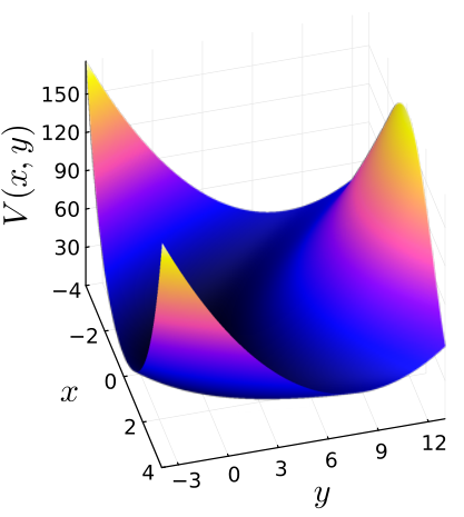
The Nelson system Baranger and Davies 1987 is described by a hamiltonian
| (86) |
which represents a particle of unit mass in two dimensions under the action of the Nelson potential
| (87) |
where is a parameter. The potential is illustrated in figure 11.
The classical dynamics in real time exhibits a generic mixture of stable regions within a chaotic sea as exemplified by its Poincaré section, visualized in Figure 12. Bifurcation trees of its periodic orbits have been intensively studied in Provost 1995; Provost and Brumer 1995; Ribeiro et al. 2004. The important point to be borne in mind is that the range between regular (integrable) and fully chaotic classical motion pertains to the infinite time limit. For finite time, the solutions of the Hamilton-Jacobi equation, which are the backbone of semiclassical approximations of finite time quantum evolution, make no qualitative distinction between these alternatives. In any case, it is reassuring that our full double hamiltonian formalism is successful even for the thorniest types of generic mixed systems.

Here, we simply use the Nelson system as an example of an application of our methods for a nontrivial system in two degrees of freedom. We then consider an ensemble of particles of unit mass under the action of this potential and calculate the thermodynamic averages associated with this system.
In this case, there are no analytical formulas available, and we must resort to numerical techniques in order to calculate the quantum energy spectrum. Because of this limitation, we only have access to a finite number of levels, and only the lower ones are reliable. This, in turn, will only give a reliable approximation for the thermodynamic quantities in the low temperature limit. On the other hand, the classical framework, as it is known, will give good results in the high temperature limit. Our hope is that our semiclassical approximation can join these two extremes in a satisfactory manner.
The semiclassical approximation for the energy, shown in figure 13, seems to bridge very well the high temperature limit, given by the classical result, and the low temperature one, given by the quantum result. Unfortunately, the approximation for the heat capacity seems to fail for much smaller values of , specially for , as can be seen in figure 14.
8 Discussion
Having reviewed and incremented the semiclassical approximation for the thermal Wigner function, we developed it into a numerical method that can be applied to a broad class of systems, including Hamiltonians that are not quadratic in their momenta. Even though further investigation will be required, we obtained good agreement of energy averages with the quantum results for a wide range of different systems and parameters. It is presumed that that this method can be useful for systems with many degrees of freedom, as its quadratic scaling law can keep computation tractable even for high dimensions.
The Weyl propagator employed here belongs to the class of propagators related to the original Van Vleck propagator by various Fourier transforms: All of these require the so called ’root search’. Thus, whereas one seeks trajectories with given end positions for the Van Vleck propagator, it is the centre point between the extremities of the trajectory that is prescribed in the Wigner-Weyl representation. So it is only for integrals involving the semiclassical Weyl propagator (or its Wick rotation) that one can switch from the centre to the initial or final value of the trajectory (as in Ozorio de Almeida et al. 2013) or to its midpoint, in the present instance.
Each representation illuminates a different aspect of quantum mechanics. Thus, the position representation, so far favoured by the vast majority of computations in this field Yan et al. 2019, can easily provide the probability density for positions, that is, the diagonal matrix elements of the density matrix are supplied explicitly. On the other hand, the momentum density requires a double Fourier transform over the pair of positions. In contrast, the Wigner function provides either density by a simple projection integral Ozorio de Almeida 1998, as exemplified by the momentum and position densities for the Morse system, shown in Fig. 10.
A further unique feature of the Wigner-Weyl representation is its symplectic invariance Ozorio de Almeida and Ingold 2014, that is, unitary quantum (metaplectic) transformations corresponding to classical linear canonical phase space transformations transport the Wigner function classically. Thus, the Wigner function supplies through simple projection integrals, not only the momentum probability density and the position probability density, but the probability density along any Lagrangian plane in phase space, that is, any plane where the action for any closed circuit is null. This multiple probability content of the density operator can be used to reconstruct it through multiple measurements in the process of quantum tomography Vogel and Risken 1989, but prior knowledge of the thermal Wigner function is welcome shortcut.
Acknowledgments
We thank Gabriel Lando for his advice on the numerics. Funding provided by Conselho Nacional de Desenvolvimento Científico e Tecnológico (CNPq) and Instituto Nacional de Ciência e Tecnologia de Informação Quântica is gratefully acknowledged.
Declarations
All authors certify that they have no affiliations with or involvement in any organization or entity with any financial interest or non-financial interest in the subject matter or materials discussed in this manuscript
Data Availability
The code used in this article can be found at Gil de Oliveira.
9 Wigner symbol of normal forms
In order to calculate the Wigner symbol of an operator of the form (47), it is sufficient to do so for the monomials , where . Our strategy will consist in finding a recurrence relation that allows us to calculate in terms of . As the initial term is readily obtained, the problem is solved.
For that, we first observe that, as is hermitian, must be real. Using this fact, writing , and applying Groenewold’s rule (11), we arrive at the recurrence relation
| (88) |
where . This relation is further simplified if we introduce the coordinates , defined by , in terms of which the laplacian takes the form
| (89) |
which allows us to rewrite (88) as
| (90) |
Since , and, as deduced from the recurrence relation, , we prove by induction that , which eliminates the derivative with respect to from (90). This allows us to easily obtain the first terms in the recurrence relation, which, already expressed in terms of , are given by
| (91) | ||||
We see that, in general, is a polynomial of order in , whose dominant term is , while corrections proportional to even powers of are also present.
10 Numerical Details
The calculations in this article were performed using the Julia language Bezanson et al. 2017 . The package DifferentialEquations.jl Rackauckas and Nie 2017 was used to solve the necessary differential equations in parallel. The calculations were performed on a 12th Gen Intel Core i5-12600K processor, which has 16 threads.
10.1 Morse System
The integrals related to the Morse system were performed using Gaussian quadrature. The integration region, in units of , is given by
| (92) |
Introducing the variables e , we obtain
| (93) | ||||
which can be simplified by defining . The, we have
| (94) |
The inverse transformation is then
| (95) |
which has jacobian determinant
| (96) |
which is proportional to the weight function of a Gauss-Chebyshev quadrature of the 3º kind. We therefore use this quadrature rule to perform the integration over the coordinate, while a Gauss-Legendre quadrature is used to integrate over . The advantage of Gaussian quadrature is that the integration points will be independent of , and then a single set of points can be used to compute the thermodynamic quantities over a range of temperatures. In this work, we used a grid of points to perform the integration, which corresponds to trajectories.
10.2 Nelson System
In the semiclassical calculations for the Nelson system, different techniques were used for different set of parameters.
In the case of the energy, as well as the heat with , we first performed the change of variables with
| (97) |
This transformation has unit jacobian determinant and, in terms of the new variables, we have that the classical Boltzmann’s weight is simply
| (98) |
The integration is then performed by an h-adaptive technique as described in Genz and Malik 1980; Berntsen et al. 1991. The Julia implementation can be found in Integrals.jl. We bounded the integration algorithm to use roughly integration points. We used the BS3 Bogacki and Shampine 1989; ODESolvers and Vern6 Verner 2010; ODESolvers algorithms to solve the differential equations, and the tolerances varied between and . For each , the corresponding plot took around seconds to minutes to complete.
We found that the heat capacities with were much harder to integrate. In this case, we didn’t perform a change of variables and resorted to a Monte Carlo integration method, where the integration points were sampled from the classical Boltzmann’s distribution using the Metropolis-Hastings algorithm Metropolis et al. 1953; Hastings 1970. In this case, for each , the corresponding plot took around hours to complete.
For the energy spectrum, which is used to calculate the quantum versions of the thermodynamic quantities, we used a grid of points, where spanned from to , and spanned from to . We then approximated the laplacian of the time independent Schrödinger equation through a finite differences matrix over this grid. The discretizatation of this equation gives rise to a eigenvalue equation, which can be solve through standard linear algebra libraries.
References
- Planck (1901) Planck, M.: Über das gesetz der energieverteilung im normalspectrum. Annalen der Physik 309(3), 553–563 (1901)
- Wigner (1932) Wigner, E.: On the quantum correction for thermodynamic equilibrium. Phys. Rev. 40, 749–759 (1932)
- Groenewold (1946) Groenewold, H.J.: On the principles of elementary quantum mechanics. Physica 12(7), 405–460 (1946)
- Moyal (1949) Moyal, J.E.: Quantum mechanics as a statistical theory. In: Mathematical Proceedings of the Cambridge Philosophical Society, vol. 45, pp. 99–124 (1949). Cambridge University Press
- Grossmann (1976) Grossmann, A.: Parity operator and quantization of -functions. Communications in Mathematical Physics 48, 191–194 (1976)
- Royer (1977) Royer, A.: Wigner function as the expectation value of a parity operator. Physical Review A 15(2), 449 (1977)
- Bertet et al. (2002) Bertet, P., Auffeves, A., Maioli, P., Osnaghi, S., Meunier, T., Brune, M., Raimond, J.-M., Haroche, S.: Direct measurement of the wigner function of a one-photon fock state in a cavity. Physical Review Letters 89(20), 200402 (2002)
- Ingold (2002) Ingold, G.-L.: Path integrals and their application to dissipative quantum systems. In: Coherent Evolution in Noisy Environments, pp. 1–53. Springer, Dresden (2002)
- Greiner et al. (2013) Greiner, W., Bromley, D.A., Reinhardt, J.: Field Quantization. Springer, Berlin, Heidelberg (2013)
- Yan et al. (2019) Yan, Y.-A., Liu, J., Shao, J.: A semiclassical initial-value representation for quantum propagator and boltzmann operator. Journal of Computational Chemistry 40(10), 1161–1171 (2019)
- Zhao and Miller (2002) Zhao, Y., Miller, W.H.: Semiclassical initial value representation for the boltzmann operator in thermal rate constants. The Journal of chemical physics 117(21), 9605–9610 (2002)
- Shao and Pollak (2006) Shao, J., Pollak, E.: A new time evolving gaussian series representation of the imaginary time propagator. The Journal of chemical physics 125(13) (2006)
- Liu and Miller (2006) Liu, J., Miller, W.H.: Using the thermal gaussian approximation for the boltzmann operator in semiclassical initial value time correlation functions. The Journal of chemical physics 125(22) (2006)
- Pollak and Martin-Fierro (2007) Pollak, E., Martin-Fierro, E.: New coherent state representation for the imaginary time propagator with applications to forward-backward semiclassical initial value representations of correlation functions. The Journal of chemical physics 126(16) (2007)
- Liu and Miller (2011a) Liu, J., Miller, W.H.: An approach for generating trajectory-based dynamics which conserves the canonical distribution in the phase space formulation of quantum mechanics. i. theories. The Journal of Chemical Physics 134(10), 104101 (2011) https://doi.org/10.1063/1.3555273
- Liu and Miller (2011b) Liu, J., Miller, W.H.: An approach for generating trajectory-based dynamics which conserves the canonical distribution in the phase space formulation of quantum mechanics. ii. thermal correlation functions. The Journal of chemical physics 134(10) (2011)
- De Carvalho et al. (1999) De Carvalho, C., Cavalcanti, R., Fraga, E., Jorás, S.: Semiclassical series at finite temperature. Annals of Physics 273(1), 146–170 (1999)
- de Carvalho et al. (2000) Carvalho, C.A.A., Cavalcanti, R.M., Fraga, E.S., Jorás, S.: Semiclassical approximation to the partition function of a particle in d dimensions. Physical Review E 61(6), 6392 (2000)
- Arnol’d et al. (2013) Arnol’d, V.I., Wassermann, G., Dubrovin, B.A., Novikov, S.P., Givental’, A.B., Kirillov, A.A., Krichever, I.M.: Dynamical Systems IV: Symplectic Geometry and Its Applications. Encyclopaedia of Mathematical Sciences. Springer, Berlin, Heidelberg (2013)
- De Almeida (1988) De Almeida, A.M.O.: Hamiltonian Systems: Chaos and Quantization. Cambridge University Press, ??? (1988)
- Haroche and Raimond (2006) Haroche, S., Raimond, J.M.: Exploring the Quantum: Atoms, Cavities, and Photons. Oxford Graduate Texts. OUP, Oxford (2006)
- Schlagheck et al. (2019) Schlagheck, P., Ullmo, D., Urbina, J.D., Richter, K., Tomsovic, S.: Enhancement of many-body quantum interference in chaotic bosonic systems: The role of symmetry and dynamics. Physical Review Letters 123(21), 215302 (2019)
- Ozorio de Almeida et al. (2021) Ozorio de Almeida, A.M., Ingold, G.-L., Brodier, O.: The quantum canonical ensemble in phase space. Physica D: Nonlinear Phenomena 424, 132951 (2021)
- Gil de Oliveira (2023) Gil de Oliveira, M.: Aproximações Semiclássicas para o Ensemble Canônico. Master’s thesis, CBPF (2023)
- Ozorio de Almeida (1998) Ozorio de Almeida, A.M.: The Weyl representation in classical and quantum mechanics. Physics reports 295(6), 265–342 (1998)
- Ozorio de Almeida and Ingold (2014) Ozorio de Almeida, A.M., Ingold, G.-L.: Metaplectic sheets and caustic traversals in the Weyl representation. Journal of Physics A: Mathematical and Theoretical 47(10), 105303 (2014)
- Nicacio et al. (2017) Nicacio, F., Valdés-Hernández, A., Majtey, A.P., Toscano, F.: Unified framework to determine gaussian states in continuous-variable systems. Physical Review A 96(4), 042341 (2017)
- Arnol’d (2013) Arnol’d, V.I.: Mathematical Methods of Classical Mechanics vol. 60. Springer, New York (2013)
- Ozorio de Almeida et al. (2013) Ozorio de Almeida, A.M., Vallejos, R.O., Zambrano, E.: Initial or final values for semiclassical evolutions in the weyl–wigner representation. Journal of Physics A: Mathematical and Theoretical 46(13), 135304 (2013)
- Yurke and Stoler (1986) Yurke, B., Stoler, D.: Generating quantum mechanical superpositions of macroscopically distinguishable states via amplitude dispersion. Phys. Rev. Lett. 57, 13–16 (1986)
- Averbukh and Perelman (1989) Averbukh, I.S., Perelman, N.F.: Fractional revivals: Universality in the long-term evolution of quantum wave packets beyond the correspondence principle dynamics. Physics Letters A 139(9), 449–453 (1989)
- Kirchmair et al. (2013) Kirchmair, G., Vlastakis, B., Leghtas, Z., Nigg, S.E., Paik, H., Ginossar, E., Mirrahimi, M., Frunzio, L., Girvin, S.M., Schoelkopf, R.J.: Observation of quantum state collapse and revival due to the single-photon Kerr effect. Nature 495(7440), 205–209 (2013)
- Lando et al. (2019) Lando, G.M., Vallejos, R.O., Ingold, G.-L., Ozorio de Almeida, A.M.: Quantum revival patterns from classical phase-space trajectories. Phys. Rev. A 99, 042125 (2019)
- de Almeida et al. (2009) Almeida, A.O., M Rios, P., Brodier, O.: Semiclassical evolution of dissipative markovian systems. Journal of Physics A: Mathematical and Theoretical 42(6), 065306 (2009)
- Brodier and de Almeida (2010) Brodier, O., Almeida, A.O.: Complex wkb evolution of markovian open systems. Journal of Physics A: Mathematical and Theoretical 43(50), 505308 (2010)
- Koda (2015) Koda, S.-i.: Initial-value semiclassical propagators for the wigner phase space representation: Formulation based on the interpretation of the moyal equation as a schrödinger equation. The Journal of Chemical Physics 143(24) (2015)
- De Aguiar et al. (2005) De Aguiar, M., Baranger, M., Jaubert, L., Parisio, F., Ribeiro, A.D.: Semiclassical propagation of wavepackets with complex and real trajectories. Journal of Physics A: Mathematical and General 38(21), 4645 (2005)
- Morse (1929) Morse, P.M.: Diatomic molecules according to the wave mechanics. ii. vibrational levels. Phys. Rev. 34, 57–64 (1929)
- Slater (1957) Slater, N.: Classical motion under a morse potential. Nature 180(4598), 1352–1353 (1957)
- Goggin and Milonni (1988) Goggin, M.E., Milonni, P.W.: Driven morse oscillator: Classical chaos, quantum theory, and photodissociation. Phys. Rev. A 37, 796–806 (1988)
- Dahl and Springborg (1988) Dahl, J.P., Springborg, M.: The Morse oscillator in position space, momentum space, and phase space. The Journal of chemical physics 88(7), 4535–4547 (1988)
- Haynes (2016) Haynes, W.M.: CRC Handbook of Chemistry and Physics. CRC Press, Boca Raton (2016)
- Riganelli et al. (2001) Riganelli, A., Prudente, F.V., Varandas, A.J.: On the rovibrational partition function of molecular hydrogen at high temperatures. The Journal of Physical Chemistry A 105(41), 9518–9521 (2001)
- Baranger and Davies (1987) Baranger, M., Davies, K.T.R.: Periodic trajectories for a two-dimensional nonintegrable hamiltonian. Annals of Physics 177(2), 330–358 (1987)
- Provost (1995) Provost, D.: Signatures of classical periodic orbits on a smooth quantum system. Physical Review E 51(6), 5396 (1995)
- Provost and Brumer (1995) Provost, D., Brumer, P.: Uniform semiclassical wave-packet propagation and eigenstate extraction in a smooth chaotic system. Physical review letters 74(2), 250 (1995)
- Ribeiro et al. (2004) Ribeiro, A., Aguiar, M., Baranger, M.: Semiclassical approximations based on complex trajectories. Physical Review E 69(6), 066204 (2004)
- Vogel and Risken (1989) Vogel, K., Risken, H.: Determination of quasiprobability distributions in terms of probability distributions for the rotated quadrature phase. Phys. Rev. A 40, 2847–2849 (1989) https://doi.org/10.1103/PhysRevA.40.2847
- (49) Gil de Oliveira, M.: GitHub repository containing the code used in this article. https://github.com/marcsgil/SCCEPaper
- Bezanson et al. (2017) Bezanson, J., Edelman, A., Karpinski, S., Shah, V.B.: Julia: A fresh approach to numerical computing. SIAM Review 59(1), 65–98 (2017) https://doi.org/10.1137/141000671
- Rackauckas and Nie (2017) Rackauckas, C., Nie, Q.: Differentialequations.jl – a performant and feature-rich ecosystem for solving differential equations in Julia. The Journal of Open Research Software 5(1) (2017) https://doi.org/10.5334/jors.151 . Exported from https://app.dimensions.ai on 2019/05/05
- Genz and Malik (1980) Genz, A.C., Malik, A.A.: Remarks on algorithm 006: An adaptive algorithm for numerical integration over an n-dimensional rectangular region. Journal of Computational and Applied mathematics 6(4), 295–302 (1980)
- Berntsen et al. (1991) Berntsen, J., Espelid, T.O., Genz, A.: An adaptive algorithm for the approximate calculation of multiple integrals. ACM Transactions on Mathematical Software (TOMS) 17(4), 437–451 (1991)
- (54) Integrals.jl. https://github.com/SciML/Integrals.jl
- Bogacki and Shampine (1989) Bogacki, P., Shampine, L.F.: A 3(2) pair of Runge - Kutta formulas. Applied Mathematics Letters 2(4), 321–325 (1989) https://doi.org/10.1016/0893-9659(89)90079-7
- (56) List of ODE Solvers of the DifferentialEquations.jl package. https://docs.sciml.ai/DiffEqDocs/stable/solvers/ode_solve/#Full-List-of-Methods
- Verner (2010) Verner, J.: Numerically optimal Runge-Kutta pairs with interpolants. Numerical Algorithms 53, 383–396 (2010) https://doi.org/10.1007/s11075-009-9290-3
- Metropolis et al. (1953) Metropolis, N., Rosenbluth, A.W., Rosenbluth, M.N., Teller, A.H., Teller, E.: Equation of state calculations by fast computing machines. The journal of chemical physics 21(6), 1087–1092 (1953)
- Hastings (1970) Hastings, W.K.: Monte carlo sampling methods using markov chains and their applications. Biometrika 57(1), 97–109 (1970)