∎
The sum of root-leaf distance interdiction problem with cardinality constraint by upgrading edges on trees
Abstract
A network for the transportation of supplies can be described as a rooted tree with a weight of a degree of congestion for each edge. We take the sum of root-leaf distance (SRD) on a rooted tree as the whole degree of congestion of the tree. Hence, we consider the SRD interdiction problem on trees with cardinality constraint by upgrading edges (denoted by (SDIPTC) in brief). It aims to maximize the SRD by upgrading the weights of critical edges such that the total upgrade cost under some measurement is upper-bounded by a given value. The relevant minimum cost problem(MCSDIPTC) aims to minimize the total upgrade cost on the premise that the SRD is lower-bounded by a given value. We develop two different norms including weighted norm and weighted bottleneck Hamming distance to measure the upgrade cost. We propose two binary search algorithms within O() time for the problems (SDIPTC) under the two norms, respectively. For problems (MCSDIPTC),we propose two binary search algorithms within O() and O() under weighted norm and weighted bottleneck Hamming distance, respectively. These problems are solved through their subproblems (SDIPT) and (MCSDIPT), in which we ignore the cardinality constraint on the number of upgraded edges. Finally, we design numerical experiments to show the effectiveness of these algorithms.
Keywords:
Network interdiction problems Tree Greedy algorithm Binary search method norm Bottleneck Hamming distanceMSC
90C27 90C351 Introduction
Terrorism is a persistent challenge for many nations worldwide, and it is imperative that governments take appropriate measures to prevent and mitigate the impact of terrorist attacks. Among the diverse tactics used by terrorists, actions that trigger fires and hinder the aid process are recognized as Network Interdiction Problems (NIPs), which are based on game theory.
An NIP involves two main actors, a leader and a follower, who have competing objectives. The follower aims to optimize their objectives by using a network to facilitate the movement of resources such as supply convoys or maximizing the amount of material transported through the network. Conversely, the leader seeks to impede the follower’s objectives by disrupting the network’s structure through interdicting arcs or nodes. The leader can do so by attacking nodes to reduce their capacity or destroy them, ultimately hindering the follower’s ability to move through the network ref1.
Some transportation networks can be represented as rooted trees with weighted edges, where the root node is the critical infrastructure or facility that the leader intends to attack, the internal nodes are served as transportation hubs, and leaf nodes are emergency agencies including fire stations, police stations, hospitals etc. The edge weight indicates the degree of congestion of the roads, and targeting these edges can disrupt the network by impeding rescue. However, decision-makers with limited resources must identify the most strategic edges to attack in order to maximize the network’s overall performance degradation.
In a broader sense, tree networks can be used to describe networks with one-directional links. For instance, during wartime, ammunition supplies may only flow from logistics centers to the front lines. The related issues can be formulated as follows.
Let be an edge-weighted tree rooted at , where and are the sets of nodes and edges, respectively. Let be the set of leaf nodes. Let and be the original weight and upper bound of edge , respectively, where . Let be the unit modification cost of edge . Let be the root-leaf path from the root node to the leaf node . Let and be the weight of the path and the sum of root-leaf distance (SRD) under the edge weight , respectively. The sum of root-leaf distance interdiction problem on trees with cardinality constraint (SDIPTC) aims to maximize the SRD by determining an edge weight vector such that the modification cost in a certain norm and the number of updated edges do not exceed two given values and , respectively. Its mathematical model can be stated as follows.
| (SDIPTC) | (1) | ||||
where is the Hamming distance between and .
We also consider its relevant minimum cost problem with cardinality constraint (MCSDIPTC) by exchanging its objective function and the norm constraint. The mathematical model of the problem is as follows.
| (MCSDIPTC) | (2) | ||||
Most network interdiction problems aim to make the network’s performance as poor as possible by deleting critical edges or nodes. Albert (2000) ref2 found that in a scale-free network when the most connected nodes are removed, the diameter of the network rapidly increases. They pointed out that this vulnerability that is susceptible to attack is due to the uneven distribution of connections and the removal of a limited number of nodes in the network can have a significant impact, giving rise to the concept of critical nodes and critical edges. Subsequently, Ayyildiz et al. (2019) ref3 analyzed how to maximize the length of the shortest path between two nodes based on a limited interdicting budget from two opposing aspects (breaking and maintaining the network). On the other hand, Magnouche and Martin (2020) ref4 studied how to delete the minimum number of critical nodes to make the root-leaf path length in the remaining graph at least . They proved the -hardness of the problem, proposed an integer linear programming model with an exponent constraints and designed a branch and bound algorithm.
Corley and Sha (1982) ref5 first applied the NIP by deleting critical edges to maximize the length of the shortest path. Ball et al. (1989) ref6 proved that the problem is -hard. Khachiyan et al. (2008) ref7 proved that there is no approximation algorithm with a performance ratio of 2. Bazgan et al. (2015) ref8 provided an time algorithm when the increment of the path length, and further (2019) ref9 proved that the problem is -hard when .
However, it is often difficult to implement the deletion of critical edges/nodes in practical applications. Zhang et al. (2021) ref10 proposed a concept of updating critical edges to replace the limitations of the traditional NIP caused by deleting critical edges, and studied the shortest path interdiction problem (SPIT) and its minimum cost problem (MCSPIT) on trees. For the problem (SPIT), they provided an primal-dual algorithm under the weighted norm and improved the time complexity to under the unit norm. For the problem (SPITuH) under unit Hamming distance, they ref11 devised algorithms with time complexities and when and , respectively, where , and are the numbers of tree nodes, upgraded edges and leaves respectively. Afterward, Yi et al. (2023) ref14 improved the time complexities to and , respectively. For the relevant minimum cost problem (MCSPITuH), based on dynamic programming ideas and binary search methods, Zhang et al. (2020) ref11 provided an algorithm. Yi et al. (2023)ref14 improved the complexity to through a binary search. Zhang et al. (2020) ref11 subsequently demonstrated that the problems (SPITH) and (MCSPITH) under the weighted Hamming distance are equivalent to the 0-1 knapsack problem and therefore -hard. Furthermore, for the SRD interdiction problems (SDIPT-UE/N) and (MCSDIPT-UE/N) by upgrading edges/nodes under weighted Hamming distance, Zhang et al. ref12 proved its -hardness by showing the equivalence between the two problems and the 0–1 knapsack problem. Under weighted norm, the problems (SDIPT1-UE) and (MCSDIPT1-UE) can be solved in time by continuous knapsack problems. For the problem (SDIPTuH-UE) under unit Hamming distance and unit node cost problem (SDIPT-UN), they designed two linear time greedy algorithms. Moreover, for the minimum cost problems (MCSDIPTuH-UE)under unit Hamming distance and unit node cost problem (MCSDIPT-UN), they ref12 used a binary search method to provide algorithms with a time complexity of .
Based on the above analysis, we can know that there is no reseach results for the SRD interdiction problems under norm and bottleneck Hamming distance, which are sub-problems of the problems (SDIPTC) and (MCSDIPTC) we mainly studied in this paper. We impose a cardinality constrain on the number of modified edges since there are always many optimal solutions, which include some unnecessary modifications of weights, for the problem (SDIPT) under bottleneck norms. We compare our results with existing studies in Table 1, where the subscripts and ∞ denote weighted -norm, unit -norm, weighted Hamming distance, unit Hamming distance, bottleneck Hamming distance, and weighted norm, respectively.
The paper is structured as follows. In Section 2, we propose two algorithms for solving problems (SDIPTC∞) and (MCSDIPTC∞) in and O() time, respectively, which mainly call the subroutines for solving the two sub-problems (SDIPT∞) and (MCSDIPT∞) in and O() time, respectively. In Section 3, we solve the problems (MCSDIPTCBH) and (SDIPTCBH) under bottleneck Hamming distance in and O() time, respectively, which have the same time complexities for the sub-problems without the cardinality constraints. In Section 4, we report on computational experiments that demonstrate the effectiveness of all proposed polynomial time algorithms. Finally, in Section 5, we summarize our findings and suggest some areas for future research.
| Type | Graph | Problem | Complexity | Ref. | |||
| Del. nodes | General graph | NIP on shortest path | any | -hard | ref4 | ||
| Del. edges | -hard | ref6 | |||||
| Not approx. within 2 | ref7 | ||||||
| Undirected network | ref8 | ||||||
| -hard | ref9 | ||||||
| Upgrad nodes | Tree | SDIPT-UN | any | any | -hard | ref12 | |
| MCSDIPT-UN | -hard | ||||||
| SDIPT-UNu | |||||||
| MCSDIPT-UNu | |||||||
| Upgrad edges | MCSPIT1 | any | c=1 | ref10 | |||
| any | |||||||
| MSPIT1 | |||||||
| any | |||||||
| MSPITH | any | -hard | |||||
| ref14 ref11 | |||||||
| any | |||||||
| MCSPITuH | |||||||
| SDIPT-UEH | any | any | -hard | ref10 | |||
| MCSDIPT-UEH | -hard | ||||||
| SDIPT-UEuH | any | c =1 | |||||
| MCSDIPT-UEuH | |||||||
| SDIPT-UE1 | any | any | |||||
| MCSDIPT-UE1 | |||||||
| SDIPT∞ | any | any | (7) | ||||
| SDIPTC∞ | Alg1 | ||||||
| MCSDIPT∞ | Alg2 | ||||||
| MCSDIPTC∞ | Alg3 | ||||||
| SDIPTBH | (26) | ||||||
| SDIPTCBH | Alg4 | ||||||
| MCSDIPTBH | Alg5 | ||||||
| MCSDIPTCBH | Alg6 | ||||||
2 Solve the problems (SDIPTC∞) and (MCSDIPTC∞) under weighted norm
When the weighted norm is applied to the upgrade cost, the problems (SDIPTC∞) and (MCSDIPTC∞) under weighted norm, can be formulated as the following models (3) and (4), respectively.
| (SDIPTC∞) | (3) | ||||
| (MCSDIPTC∞) | (4) | ||||
This section proves the properties of the problem (SDIPTC∞) and presents a divide-and-conquer algorithm with time complexity of for it. For the relevant minimum cost problem (MCSDIPTC∞), this section provides an algorithm with a time complexity of .
Definition 1
ref12 For any , define as the set of leaves to which passes through . If , then is controlled by the edge .
2.1 An time algorithm to solve the problem (SDIPTC∞)
In order to solve problem (SDIPTC∞), we first consider its sub-problem (SDIPT∞) by deleting the constraint of cardinality. Its mathematical model can be described as follows.
| (SDIPT∞) | (5) | ||||
In the problem (SDIPT∞), we can maximize the weight of each edge as much as possible under the constraint of cost and the upper bound of the edge weight . Therefore, we have the following theorem.
Theorem 2.1
The weight vector
| (6) |
is an optimal solution to the problem (SDIPT∞).
Proof
(1) Apparently, the solution defined by (6) satisfies feasibility.
(2) Suppose that is not the optimal solution, and there exists another edge weight vector such that . Then at least one edge satisfies . We have , which implies or , either of which contradicts the cost constraint condition or the upper bound constraint condition, respectively. Therefore, is an optimal solution to problem (SDIPT∞).
Based on Theorem 2.1, for any given , we can obtain an optimal solution and its corresponding optimal value for problem (SDIPT∞). For convenience, we denote this subroutine as:
| (7) |
We just update every edges in the subroutine, therefore, we have the following conclusion.
Theorem 2.2
Problem (SDIPT∞) can be solved by subroutine (7) in time.
Now we can come to the problem (SDIPT∞) with cardinality constraint. First, call . Then, we define , which means the increment of SRD for under . Based on that, we can select the edges with the largest , and update them to obtain an optimal solution.
Therefore, in the first step, we use the algorithm proposed by Thoms (2009, pp.220-222) ref13 called to find the -th largest element in the set , and thus divide the edge set into two parts, and .
Theorem 2.3
The weight vector
| (8) |
is an optimal solution of the problem (SDIPTC∞).
Proof
Feasibility is obviously satisfied. Suppose is not optimal, but is. Then , and there exists at least one edge , such that .
(1) If , then , which contradicts the upper bound or update cost constraints.
(2) If , then . Moreover, there must exist an edge in such that . Since , there exists a feasible solution given by
thus we have
this indicates that , which contradicts the optimality of .
Theorem 2.4
Problem (SDIPTC∞) can be solved by Algorithm 1 in time.
2.2 An time algorithm to solve the problem (MCSDIPTC∞)
Solving problem (MCSDIPTC∞) directly is challenging, and therefore, we first focus on solving its sub-problem (MCSDIPT∞) without the cardinality constraint. This sub-problem can be described as follows:
| (MCSDIPT∞) | (9) | ||||
For convenience, let .
2.2.1 An algorithm to solve (MCSDIPT∞)
For the problem (MCSDIPT∞), we can solve two special cases based on the relationship between and , as well as and .
Lemma 1
If , then is an optimal solution to (MCSDIPT∞).
Lemma 2
If , then the problem (MCSDIPT∞) is infeasible.
The proofs of the above two lemmas are obvious. Then we consider the situation that . First, we will prove an interesting property of the optimal solution.
Lemma 3
Let be an optimal solution of problem (MCSDIPT∞), then .
Proof
Suppose SRD under optimal solution is . Let ), then
while the maximum cost
which contradicts the optimality of .
Here we construct an optimal solution to the problem (MCSDIPT∞) where . Using the property of the norm, we know that when the update costs are fixed, updating every edge can increase SRD by the maximum amount. For each edge , let represent the total cost required to achieve the maximum possible update. Then we sort the values of all edges in a non-decreasing order and renumber them to obtain the sequence as follows:
| (10) |
For an index , define a function
| (11) |
to represent the maximum increment of SRD when the update cost is
Next, using the binary search method on the sequence , we can determine a critical index such that . This allows us to obtain a unique optimal solution to the problem (MCSDIPT∞).
Theorem 2.5
When , let , the weight vector
| (12) |
is the unique optimal solution to the problem (MCSDIPT∞),
Proof
(1) First, we prove that is a feasible solution to problem MCSDIPT∞.
(1.1) We prove that for satisfies the bound constraint. When , we have ; and when , we have .Then
Therefore
Hence, , for any .
(1.2) Prove that under , .
Therefore, , and is a feasible solution to problem MCSDIPT∞.
(2) Next, we prove the optimality of .
Assume that is not the optimal solution of problem (MCSDIPT∞), but is. Then there exists such that . Therefore, the total increment in SRD due to edge is . According to Lemma 3, and , there exists an edge such that , which implies that .
(2.1) If , then , which contradicts the feasibility of .
(2.2) If , then , which contradicts .
Therefore, is the optimal solution to the problem (MCSDIPT∞).
(3) We prove the uniqueness of by contradiction
Suppose is another optimal solution of the problem (MCSDIPT∞), such that and there exists such that .
(3.1) If , then we have , and we can construct a feasible solution , where . Thus we construct another feasible solution , we get , which contradicts the optimality of .
(3.2) If and , then , which contradicts to the optimality of . Suppose , similarly we can construct a feasible solution , where .
Then we construct , now we have and , which contradicts to the optimality of .
In conclusion, the weight vector defined by (12) is the unique optimal solution to the problem (MCSDIPT∞).
Theorem 2.6
The problem (MCSDIPT∞) can be solved by Algorithm 2 in time.
Proof
The sorting in Line 8 can be completed in time. The binary search process in Lines 10-21 takes iterations. So it takes a total of time. Therefore, the problem (MCSDIPT∞) can be solved in time.
2.2.2 An algorithm to solve (MCSDIPTC∞)
For the original problem (MCSDIPTC∞), we first consider its feasibility. We define , which represents the maximum increment in SRD that each edge can achieve. We sort the edges in a non-increasing order of and renumber them to obtain the following sequence:
| (13) |
Under the cardinality constraint of edges, the maximum total increment in SRD is .
If , then it is clear that the problem has no solution, as the increment is not sufficient to meet the problem requirements.
Lemma 4
When , problem (MCSDIPTC∞) is infeasible.
When , we give the following lemma to determine the number of edges that are updated in any optimal solution.
Lemma 5
Suppose , and let be an optimal solution of problem (MCSDIPTC∞). Let . Then, we have
Proof
(1) When , it means that the cardinality constraint is always satisfied. So the problem (MCSDIPTC∞) can be directly transformed to its sub-problem (MCSDIPT∞). According to Theorem 2.5, all edges will be updated, so in this case.
(2) When , we prove by contradiction. Suppose that . Then, there is an edge such that . We can construct a solution , where . Then and thus
| (14) | |||||
Let , we can construct a solution
then we have
where the last equality can be obtained from (14). Furthermore, note that
then is a feasible solution. However, it follows from the definitions of and that , which contradicts the optimality of .
Based on the analysis above, if we can determine the set of edges that are updated in the optimal solution, then the problem (MCSDIPTC∞) can be transformed into its sub-problem (MCSDIPT∞) which can be solved by Algorithm 2 in time. Next, we use an iterative method to determine the set .
Initialization: , .
Call Algorithm 2: =MCSDIPT, where , then the obtained is the initial feasible solution and the corresponding objective value of the problem.
Next, for each edge in the current edge set , consider whether there exists a better edge in the set that can reduce the upgrade cost by replacing it.
Sort the values in a non-increasing order such that
| (15) |
Let denote the maximum SRD increment of edge within the maximum cost .
Let be the set of edges whose costs reach . For edge and edge , where is traversed according to the sequence , there are two replacement scenarios as follows.
(1) If , and . Then is replaced with and update .
(2) If and , then is replaced with and .
After the replacement is done for all and , set , the first iteration is finished.
In the second iteration, let and call Algorithm 2: =MCSDIPT. The resulting is a better feasible solution to problem (MCSDIPTC∞) than , with a corresponding objective value of .
Theorem 2.7
The solution is feasible to problem (MCSDIPTC∞), and .
Proof
Without loss of generality, let where and .
(1) If , then
| (16) | |||
| (17) |
(1.1) Use induction to prove the feasibility of . First, since , the vector is a feasible solution to the original problem.
Assume that the feasibility holds when then
which means that and . Thus we can get a feasible solution after calling Algorithm 2, which satisfies . Furthermore, , and for any edge , , so is a feasible solution to problem (MCSDIPTC∞).
(1.2) We show by contradiction. Assume . Then, . Also, by Lemma 3, we have which implies that
Therefore,
| (18) |
Then, for any edge , , combined with the assumption , we have
It follows from (19) that
which implies that
Therefore, we have , which contradicts equation (17).
(2) If , then . Using the same argument as (1.1), we can prove that is a feasible solution for problem (MCSDIPTC∞). Next, we show by contradiction. Similar to (1.2), we have equation (18). However, this contradicts the fact that .
Then, update and continue iterating until there is no edge in better than any edge in the current set . Denote the resulting set of edges by . Let Then, call Algorithm 2:
| (20) |
Theorem 2.8
The solution obtained by (20) is an optimal solution to problem (MCSDIPTC∞).
Proof
According to Theorem 2.7, the iteratively obtained solution is feasible.
Assume that is not optimal, but is, such that .
Let , , , , and .

(1) If , then by the uniqueness of the optimal solution of the problem (MCSDIPT∞), we have , which contradicts the assumption.
(2) If , since , we have . Therefore, the total increment in SRD on by should be no more than that by and . Moreover, since and , we have
| (21) |
(2.1) If “” holds in equation (21), then there exist and such that , which implies that .
From the replacement case (2) of the iteration , it can be concluded that at the end of the iteration, for each edge in under , there is no edge in that can replace any edge in . However, the contradiction arises from the fact that and edge satisfies the replacement requirement of edge .
(2.2) If the equality holds in (21), it means that the two edge weight vectors achieve the same SRD on the same edge set . Due to the uniqueness of the optimal solution of the problem (MCSDIPT∞), it follows that SRD increment by each edge in must be equal. Therefore, the maximum cost edges of the two schemes are in and , respectively. Moreover, since , it follows that is better than , and there must be at least one edge , such that and edge satisfies the replacement requirement of edge , which leads to a contradiction.
Therefore, is the optimal solution to the original problem.
The following Algorithm 3 can be obtained from the above analysis to solve the problem (MCSDIPT∞).
Theorem 2.9
Problem (MCSDIPTC∞) can be solved by Algorithm 3 in time.
Proof
In Algorithm 3, we sort and in Lines 2 and 7, which takes a total of time. In the loop from Line 10 to 31, Line 13 calculates the optimal solution and for the problem (MCSDIPT∞) obtained by modifying only edges in , which requires time according to Theorem 2.6. In the loop from Line 15 to 29, we iterate over the sets and , which takes iterations. In each iteration we can update the selected edges in time. Therefore, problem (MCSDIPT∞) can be solved by Algorithm 3 in time.
3 Solve the problems (SDIPTCBH) and (MCSDIPTCBH) under weighted bottleneck Hamming distance
When the weighted bottleneck Hamming distance is applied to the upgrade cost, the problems (SDIPTCBH) and (MCSDIPTCBH) can be formulated as the following models (22) and (23), respectively.
| (SDIPTCBH) | (22) | ||||
| (MCSDIPTCBH) | (23) | ||||
In this section, we first provide an algorithm with time complexity for problem (SDIPTCBH). For the minimum cost problem (MCSDIPTCBH), we transform it into its sub-problem (MCSDIPTBH) and provide an algorithm with time complexity .
3.1 An time algorithm to solve the problem (SDIPTCBH)
Similarly, we first consider solving the sub-problem (SDIPTBH) without the cardinality constraint, which can be formulated as follows.
| (SDIPTBH) | (24) | ||||
Based on the characteristic of bottleneck Hamming distance, in order to maximize the objective function, we consider updating the edges that satisfy . Thus, we give the following optimality condition.
Theorem 3.1
The weight vector
| (25) |
is an optimal solution to problem (SDIPTBH).
Proof
Clearly, is a feasible solution to problem (SDIPTBH). Suppose that is not the optimal solution, but is. Then, there must be at least one edge such that . If , we have , which contradicts . If , the cost should be at least , which is greater than the cost limit , contradicting the assumption. Therefore, the defined in (25) is the optimal solution to problem (SDIPTBH).
Based on Theorem 3.1, for any given , we can obtain an optimal solution and its corresponding optimal value for the problem (SDIPTBH). For convenience, we denote this subroutine as:
| (26) |
Obviously, this problem only requires one traversal of , so we have the following conclusion.
Theorem 3.2
The subroutine (26) can solve problem (SDIPTBH) in time.
Then we consider the original problem (SDIPTCBH). Similar to problem (SDIPTBH), we can partition into two parts and . Then, we select elements in according to the value of . Depending on the relationship between and the cardinality constraint , we divide the problem into the following two cases and solve them. The first case is rather simple.
Lemma 6
When ,the weight vector is an optimal solution to problem (SDIPTCBH).
When , we first prioritize the edges with larger values in the set . We use the algorithm ref13 to select the -th largest element from . Based on this, we divide the set into and .
Theorem 3.3
When , the weight vector
| (27) |
is an optimal solution to problem (SDIPTCBH).
Proof
Obviously, is a feasible solution for problem (SDIPTCBH). Suppose is not optimal, while is. Then we have and there exists at least one edge such that .
If , we have , which contradicts the upper bound constraint.
If and , we have , which contradicts the updated cost limit.
If and , since , there must exist an edge such that . Moreover, since for all , we have . In this case, we can construct a new edge weight vector as follows:
and we have , which contradicts the assumption.
Similar to the proof of Theorem 2.4, we have the following lemma.
Lemma 7
Problem (SDIPTCBH) can be solved by Algorithm 4 in time.
3.2 An time algorithm to solve the problem (MCSDIPTCBH)
Concerning problem (MCSDIPTCBH), similarly, we first consider its sub-problem (MCSDIPTBH) without cardinality constraint, which can be formulated as follows.
| (MCSDIPTBH) | (28) | ||||
According to the relationship between and , as well as and , we discuss the following two cases of the problem separately.
Lemma 8
When , problem (MCSDIPTBH) is infeasible.
Lemma 9
If , then is an optimal solution to (MCSDIPTBH).
When , we first sort the edges in an ascending order by their values and renumber them in the following sequence
| (29) |
Let , and we then construct an auxiliary function
| (30) |
which represents the SDR added when updating the first edges in the sequence . We use a binary search method to iteratively determine such that and give the following conclusion.
Theorem 3.4
If , then the weight vector defined by:
| (31) |
is an optimal solution to (MCSDIPTBH). Here, .
Proof
It is obvious that is feasible to the problem (MCSDIPTBH). Suppose is not optimal, but is. Then . Let and be the edges in the sequence with the maximum cost in and respectively. Then , so . Since is the smallest index satisfying , thus , which contradicts the optimality of .
The following lemma follows from the time complexity of Theorem 2.6.
Lemma 10
Problem (MCSDIPTBH) can be solved by Algorithm 5 in time.
Now we can consider solving the cardinality problem (MCSDIPTCBH). First, we need to determine the infeasibility by Lemma 4 similarly.
Lemma 11
When , problem (MCSDIPTCBH) is infeasible.
When , we first run Algorithm 5:
to obtain the optimal solution to its sub-problem (MCSDIPTBH). This leads to the following lemma.
Lemma 12
If and , then is the optimal solution to problem (MCSDIPTCBH).
If , sort the edges in a non-decreasing order according to their values by (29). For any , let , , call ref13. Let , then
| (32) |
is the maximum SDR that can be increased by updating edges among the first edges in the sequence .
Next, we can use binary search for iteration to find the smallest such that , and let the updated edge set at this point be .
Theorem 3.5
If , the weight vector
| (33) |
is an optimal solution to problem (MCSDIPTCBH).
Proof
It is obvious that is a feasible solution to problem (MCSDIPTCBH). Assume that is not optimal, and is an optimal solution with . Suppose that the updated edges in correspond to the sequence satisfying . It is clear that and since satisfies . This contradicts the assumption that is the smallest value satisfying .
Theorem 3.6
Problem (MCSDIPTCBH) can be solved by Algorithm 6 in time.
Proof
In Algorithm 6, we sort and in Lines 2 and 11, which takes time. Furthermore, in the loop from Line 13 to 23, we use the algorithm to calculate in Line 15, which takes time ref13, and the whole loop is searched using binary search, so it can be completed in time. Therefore, problem (MCSDIPTCBH) can be solved by Algorithm 6 in time.
4 Numerical Experiments
4.1 An example to show the process of Algorithm 3 and 6
For the better understanding of Algorithm 3 and 6, Example 1 is given to show the detailed computing process.
Example 1
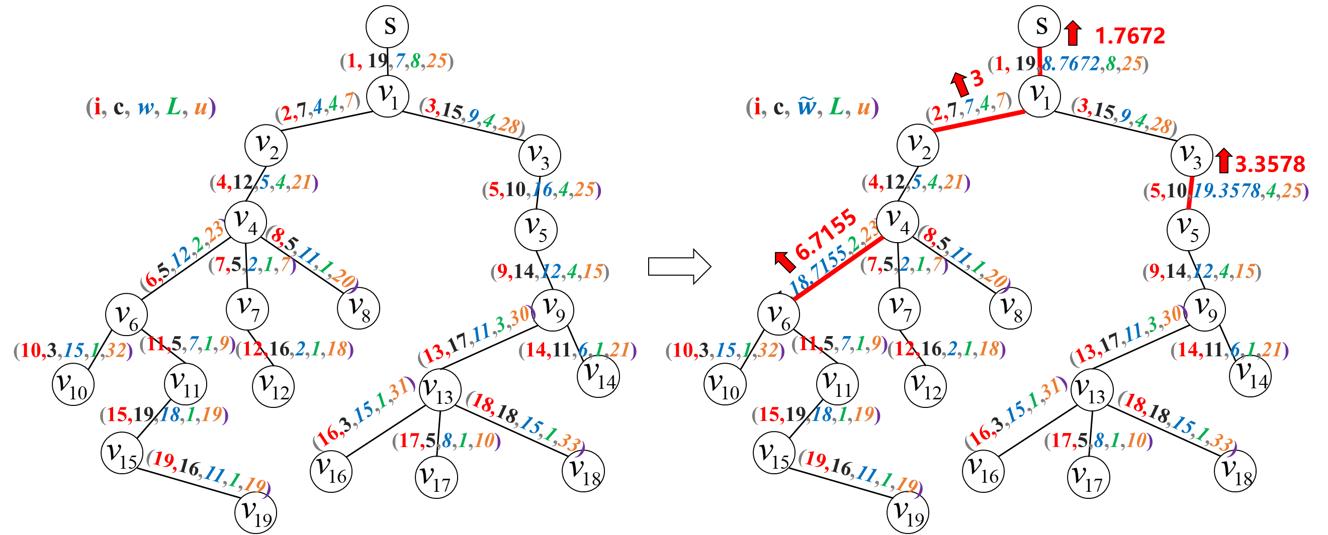
4.1.1 Execution of Alg. 3
(1) By defining , the values of are sorted in a non-increasing order, resulting in . As , the problem is feasible and has a valid solution.
(2) The values of are calculated and sorted in non-increasing order.
(3) The algorithm is initialized with , , .
(4) The cycle process is presented in the following table 2.
| (9.3294, 11.9505, 8.6882, 13.6034) | |||
| (9.3182, 7.0000, 8.6705, 13.5909) | |||
| (9.1633, 7.0000, 20.1102, 13.4178) | |||
| (8.7672, 7.0000, 19.3578, 18.7155) | |||
| (8.7672, 7.0000, 19.3578, 18.7155) |
Finally, we get the optimal value . It is worth noting that in the first cycle, we updated the edge set three times with different values on Table 2. Algorithm 2 was called only once at the beginning. We show the upgraded weights of 4 edges on the right figure in Fig. 2.
4.1.2 Execution of Alg. 6
(1) Similarly, sort in non-increasing order, resulting in . As , the problem is feasible and has a valid solution.
(2) MCSDIPT, and we get , so and .
(3) , we get .
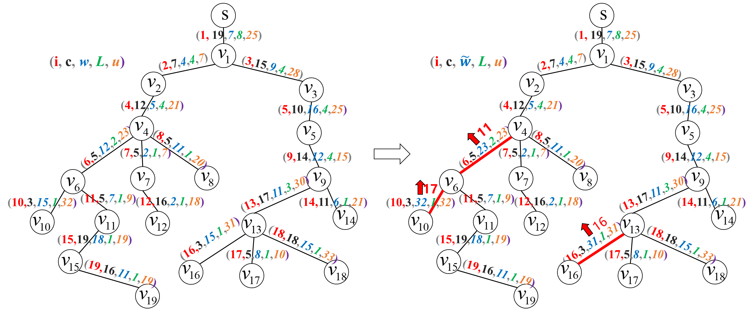
4.2 Computational experiments
We present the numerical experimental results for formulas (7), (26), and algorithms 1-6 in Table 3. These programs were coded in Matlab2021a and ran on an Intel(R) Core(TM) i7-10875H CPU @ 2.30GHz and 2.30 GHz machine running Windows 11. We tested these algorithms on six randomly generated trees with vertex numbers ranging from 1000 to 50000. We randomly generated the vectors , and such that and . We randomly generated , and for the problems (SDIPT), (MCSDIPT), (SDIPTC, MCSDIPTC), respectively. For each randomly generated tree , vectors , , , and values and , we tested formulas (7), (26), and algorithms 1-6, whose average, maximum and minimum CPU time are denoted by , and , respectively, where .
From Table 3, we can see that Algorithm 3 is the most time-consuming due to the complexity of its program and the uncertainty of its iteration number. Formulas (7) and (26) are relatively simple and require only one traversal of the vector, so they are less time-consuming.
Overall, these algorithms are all very effective and follow their respective time complexities well. When is small, the time differences among the three algorithms are relatively small, but as increases, the differences between the algorithms become more pronounced.
| Complexity | 1000 | 5000 | 10000 | 30000 | 50000 | |
| 0.0002 | 0.0003 | 0.0005 | 0.0013 | 0.0019 | ||
| 0.0005 | 0.0021 | 0.0038 | 0.0107 | 0.0186 | ||
| 0.0001 | 0.0001 | 0.0002 | 0.0007 | 0.0014 | ||
| 0.0008 | 0.0037 | 0.0084 | 0.0251 | 0.0393 | ||
| 0.0022 | 0.0079 | 0.0095 | 0.0274 | 0.0428 | ||
| 0.0003 | 0.0017 | 0.0029 | 0.0160 | 0.0251 | ||
| 0.0013 | 0.0062 | 0.0140 | 0.0679 | 0.1477 | ||
| 0.0075 | 0.0122 | 0.0217 | 0.0805 | 0.1802 | ||
| 0.0010 | 0.0036 | 0.0109 | 0.0561 | 0.1365 | ||
| 0.0004 | 0.0612 | 0.3575 | 11.24 | 47.66 | ||
| 0.0013 | 0.0682 | 0.4720 | 24.36 | 62.34 | ||
| 0.0002 | 0.0446 | 0.2654 | 6.331 | 40.98 | ||
| 0.0007 | 0.0037 | 0.0081 | 0.0246 | 0.0403 | ||
| 0.0023 | 0.0071 | 0.0100 | 0.0267 | 0.0429 | ||
| 0.0004 | 0.0031 | 0.0069 | 0.0221 | 0.0387 | ||
| 0.0012 | 0.0057 | 0.0114 | 0.0320 | 0.0715 | ||
| 0.0063 | 0.0098 | 0.0135 | 0.0493 | 0.0974 | ||
| 0.0007 | 0.0042 | 0.0096 | 0.0262 | 0.0638 | ||
| 0.0016 | 0.0067 | 0.0150 | 0.0683 | 0.1578 | ||
| 0.0064 | 0.0119 | 0.0413 | 0.0893 | 0.1917 | ||
| 0.0008 | 0.0052 | 0.0120 | 0.0602 | 0.1424 | ||
| 0.0021 | 0.0097 | 0.0209 | 0.0781 | 0.1792 | ||
| 0.0077 | 0.0141 | 0.0425 | 0.0914 | 0.2024 | ||
| 0.0012 | 0.0085 | 0.0187 | 0.0774 | 0.1623 |
5 Conclusion and further research
This paper proposes two linear time greedy algorithms for problems (SDIPT∞) under weighted norm and the problem (SDIPTBH) under bottleneck Hamming distance, respectively. For their relevant minimum cost problems (MCSDIPT∞) and (MCSDIPTBH), two time algorithms are proposed based on binary methods, respectively. In addition, this paper considers the sum of root-leaf distance interdiction problem with cardinality constraints by upgrading edges on trees(SDIPTC) and its relevant minimum cost problem (MCSDIPTC). Then two binary search algorithms are proposed within time for the problems (SDIPTC) under weighted norm and weighted bottleneck Hamming distance, respectively. For problems (MCSDIPTC), two binary search algorithms within and under weighted norm and weighted bottleneck Hamming distance are proposed, respectively.
We validate the effectiveness of the proposed algorithms through numerical experiments. As future work, we aim to extend our approach to interdiction problems on source-sink path length, maximum flow, and minimum spanning tree under different measurements for general graphs.
Funding The Funding was provided by National Natural Science Foundation of China (grant no: 11471073).
Data availability Data sharing is not applicable to this article as our datasets were generated randomly.
Declarations
Competing interests The authors declare that they have no competing interest.
References
- (1) Albert, R, Jeong, H, Barabási, A (2000) Error and attack tolerance of complex networks. Nature, 406(6794), 378-382.
- (2) Ayyldz E, Zelik G, Gencer CT (2019) Determining the most vital arcs on the shortest path for fire trucks in terrorist actions that will cause fire. Commun Fac Sci Univ Ankara Ser A1 Math Stat 68(1):441–450
- (3) Ball MO, Golden BL, Vohra RV (1989) Finding the most vital arcs in a network. Oper Res Lett 8(2):73–76
- (4) Bazgan C, Fluschnik T, Nichterlein A, Niedermeier R, Stahlberg M (2019) A more fine-grained complexity analysis of finding the most vital edges for undirected shortest paths. Networks 73(1):23–37
- (5) Bazgan C, Nichterlein A et al (2015) A refined complexity analysis of finding the most vital edges for undirected shortest paths. In: Algorithms and complexity: lecture notes in computer science, vol 9079, pp 47–60
- (6) Corley HW, Sha DY (1982) Most vital links and nodes in weighted networks. Oper Res Lett 1:157–161
- (7) Cormen TH, Leiserson CE, Rivest RL, et al. (2022) Introduction to algorithms. 4rd edn. MIT press.
- (8) Israeli E, Wood RK (2002). Shortest‐path network interdiction. Networks, 40(2): 97-111.
- (9) Khachiyan L, Boros E, Borys K, Elbassioni K, Gurvich V, Rudolf G, Zhao J (2008) On short paths interdiction problems: total and node-wise limited interdiction. Theory Comput Syst 43(2):204–233
- (10) Lei Y, Shao H, Wu T, et al. (2023). An accelerating algorithm for maximum shortest path interdiction problem by upgrading edges on trees under unit Hamming distance. Optim Lett 17, 453–469.
- (11) Magnouche Y, Martin S (2020) Most vital vertices for the shortest s-t path problem: complexity and Branch-and-Cut algorithm. Optim Lett 14(2):2039–2053
- (12) Zhang Q, Guan XC, Jia JH, et al. (2022). The sum of root-leaf distance interdiction problem by upgrading edges/nodes on trees. J Comb Optim, 44(1), 74-93.
- (13) Zhang Q, Guan XC, Pardalos PM (2021a) Maximum shortest path interdiction problem by upgrading edges on trees under weighted l1 norm. J Global Optim 79(4):959–987
- (14) Zhang Q, Guan XC, Wang H, Pardalos PM (2021b) Maximum shortest path interdiction problem by upgrading edges on trees under Hamming distance. Optim Lett 15(8): 2661–2680