Single Proxy Synthetic Control
Abstract
Synthetic control methods are widely used to estimate the treatment effect on a single treated unit in time-series settings. A common approach to estimate synthetic control weights is to regress the treated unit’s pre-treatment outcome and covariates’ time series measurements on those of untreated units via ordinary least squares. However, this approach can perform poorly if the pre-treatment fit is not near perfect, whether the weights are normalized or not. In this paper, we introduce a single proxy synthetic control approach, which views the outcomes of untreated units as proxies of the treatment-free potential outcome of the treated unit, a perspective we leverage to construct a valid synthetic control. Under this framework, we establish an alternative identification strategy and corresponding estimation methods for synthetic controls and the treatment effect on the treated unit. Notably, unlike existing proximal synthetic control methods, which require two types of proxies for identification, ours relies on a single type of proxy, thus facilitating its practical relevance. Additionally, we adapt a conformal inference approach to perform inference about the treatment effect, obviating the need for a large number of post-treatment observations. Lastly, our framework can accommodate time-varying covariates and nonlinear models. We demonstrate the proposed approach in a simulation study and a real-world application.
Keywords: Average treatment effect on the treated, Conformal inference, Generalized method of moments, Prediction interval, Synthetic control
1 Introduction
Synthetic control methods have grown popular for estimating the treatment effect of an intervention in settings where a single unit is treated and pre- and post-treatment time series data are available on the treated unit and a heterogeneous pool of untreated control units (Abadie and Gardeazabal 2003; Abadie et al. 2010). In the absence of a natural control unit, the main idea of the approach hinges upon constructing a so-called synthetic control, corresponding to a certain weighted average of control units’ outcomes (and potentially covariates), obtained by matching the outcome time series of the treated unit to the weighted average in the pre-intervention period, to the extent empirically feasible. The resulting synthetic control is then used to forecast the treatment-free potential outcome of the treated unit in the post-treatment period, therefore delivering an estimate of the treatment effect by comparing the treated unit’s outcome to the synthetic control forecast.
There is a fast-growing literature concerned with developing and improving approaches to constructing synthetic control weights. Following Abadie et al. 2010, a common approach is to use ordinary (or weighted) least squares by regressing the pre-treatment outcome and available covariates of the treated unit on those of control units, typically restricting the weights to be nonnegative and sum to one; see Section 2.2 for a more detailed discussion. Despite intuitive appeal and simplicity, the performance of the standard synthetic control approach may break down in settings where the pre-treatment synthetic control match to the treated unit’s outcomes is short of perfect; an eventuality Abadie et al. 2010 warns against. In order to improve the performance of the synthetic control approach in the event of an imperfect pre-treatment match, recent papers have considered alternative formulations of the synthetic control framework. For example, Xu 2017; Amjad et al. 2018; Ben-Michael et al. 2021; Ferman and Pinto 2021; Ferman 2021; Shi et al. 2023 rely on variants of a so-called interactive fixed effects model (IFEM; Bai 2009). In particular, the latter three papers specify a linear latent factor potential outcome model with an exogenous, common set of latent factors with corresponding unit-specific factor loadings. Under this linear factor model, a key identification condition is that the factor loading of the treated unit lies in the vector space spanned by factor loadings of donor units, and thus, there exists a linear combination of the latter that matches the former exactly. Using the corresponding matching weights, one can therefore construct an unbiased synthetic control of the treated unit’s potential outcome which, under certain conditions, can be used to mimic the treated unit’s outcome in the post-treatment period, had the intervention been withheld. At their core, these methods substitute the requirement of a perfect pre-treatment match of the outcome of the treated unit and the synthetic control (an empirically testable assumption) with finding a match for the treated unit’s factor loadings in the linear span of the donors’ factor loadings (an empirically untestable assumption). Despite the growing interest in synthetic control methods, limited research has gone beyond the IFEM or its nonparametric generalizations (Qiu et al. 2024; Shi et al. 2023); one notable exception is Shi et al. 2022 where the units’ outcomes are viewed as averages of more granular study units, allowing for the construction of a synthetic control under specific restrictions on the model of granular study units’ outcomes.
In this work, we consider an alternative theoretical framework to formalize the synthetic control approach which obviates a specification of an IFEM. Specifically, we propose to view the synthetic control model from a measurement error perspective, whereby donor units’ outcomes stand as error-prone proxy measurements of the treated unit’s treatment-free potential outcome. In this framework, a synthetic control outcome can be obtained via a simple form of calibration, say a linear combination of donor units, so that on average, it matches the treated unit’s outcome in the pre-treatment period. Whereas the standard IFEM views the treated and control units’ outcomes as proxies of latent factors, our approach views donor units’ outcomes as direct proxies of the treated unit’s treatment-free potential outcome. Thus, the proposed framework shares similarity with the recent proximal synthetic control framework of Shi et al. 2023, which also formalizes donor outcomes as so-called outcome proxies. However, a major distinction is that the latter requires an additional group of proxies (so-called treatment proxies) to identify synthetic control weights; in contrast, our proposed approach relies on a single type of proxies, given by donor units and obviates the need to evoke existence of latent factors.
Interestingly, similar to the connection between the proximal synthetic control approach of Shi et al. 2023 and proximal causal inference for independent and identically distributed (i.i.d.) data (Miao et al. 2018; Tchetgen Tchetgen et al. 2024), the proposed synthetic control framework is likewise inspired by the control outcome calibration approach (Tchetgen Tchetgen 2013) and its recent generalization to a so-called single proxy control framework (Park et al. 2024) both of which were proposed for i.i.d. samples subject to an endogenous treatment assignment mechanism. Therefore, we aptly refer to our approach as single proxy synthetic control (SPSC) approach. Despite this connection, the synthetic control generalization presents several new challenges related to (i) only observing a single treated unit, and therefore treatment assignment is implicitly conditioned on, and (ii) having access to pre-and post-treatment time series data for a heterogeneous pool of untreated donor units, none of which can serve as a natural control; and (iii) serial correlation and heteroskedasticity due to the time series nature of the data. We tackle each of challenges (i)-(iii) in turn and develop a general framework for single proxy control in a synthetic control setting. The proposed method is implemented in an R package available at https://github.com/qkrcks0218/SPSC.
2 Setup And Review of Existing Synthetic Control Frameworks
2.1 Setup
Let us consider a setting where units are observed over time periods. Units and time periods are indexed by and , respectively. Following the standard synthetic control setting, we suppose that only the first unit with index is treated, whereas the latter units with index are untreated control units; these untreated control units are also referred to as donors. Consider a binary treatment indicator which encodes whether time is in the pre-treatment period, in which case for , or the post-treatment period, in which case for , respectively. Thus, is the number of pre-treatment periods and is the number of post-treatment periods. Unless otherwise stated, we assume that is fixed and and are large with similar order of magnitude. Let and denote observed outcomes of the treated unit and the th control unit, respectively, for . We define as the -dimensional vector of the untreated units’ outcome at time . We define as the observed data at time . Let and denote the potential outcomes of the treated and th control units, respectively, which one would have observed had, possibly contrary to fact, the treatment been set to at time .
For illustrative purposes, we will consider the following two examples throughout:
Example 2.1.
Abadie et al. 2010 investigated the effects of Proposition 99, a tobacco control program implemented in California in 1988, on cigarette sales in the state. Their empirical analysis considered annual cigarette sales data from California and from other states, corresponding to and , respectively. The potential outcome represents California’s cigarette sales had Proposition 99 not been implemented. The data covered the period from 1970 to 2000, resulting in pre-treatment and post-treatment time periods.
Example 2.2.
In Section 5, we revisited the analysis by Fohlin and Lu 2021 to study the effects of the Panic of 1907 (Moen and Tallman 1992) on the average log stock prices of two trust companies (Knickerbocker and Trust Company of America) that were hypothesized to have been impacted by the Panic. For comparison, a selection of trust companies conjectured to be immune to the Panic served as potential control units. The log stock price of these trust companies defines and , respectively. The potential outcome represents the average log prices of Knickerbocker and Trust Company of America had the Panic of 1907 not occurred. The tri-weekly panel data consists of pre-treatment and post-treatment time periods, respectively.
Throughout, let denote the indicator function of an event , i.e., if is satisfied and otherwise. Let be the set of real numbers. Let denote that and are conditionally independent given . Conversely, we use to denote that and are conditionally dependent given . Let , , and denote the -dimensional zero matrix, -dimensional matrix with ones, and -dimensional identity matrix, respectively.
2.2 Review of Existing Synthetic Control Framework
A common target estimand in the synthetic control setting is the average treatment effect on the treated unit (ATT) at time in the post-treatment periods, i.e.,
Note that, by definition, for where is a mean-zero idiosyncratic residual error and, therefore, may be viewed as a deterministic function of time capturing the expected effect of the treatment experienced by the treated unit if one were to average over the residual . In Section 3.5, we describe an approach for constructing prediction intervals for by appropriately accounting for the idiosyncratic error term . To proceed, we make the consistency assumption:
Assumption 2.1 (Consistency).
almost surely and almost surely for all and .
Additionally, we assume no interference, i.e., the treatment has no causal effect on control units.
Assumption 2.2 (No Interference on Control Units).
almost surely for all and .
In the context of Example 2.1, Assumption 2.2 means that Proposition 99 does not have a causal effect on other states’ cigarette sales; a similar interpretation applies to Example 2.2.
Under Assumptions 2.1 and 2.2, we have the following result almost surely for :
Therefore, for the post-treatment period, matches the observed outcome while is unobserved, implying that an additional assumption is required to establish identification of the ATT.
In the classical synthetic control setting, a further assumption relates the observed outcomes of the untreated units with the treatment-free potential outcome of the treated unit. Specifically, following Abadie et al. 2010 and Ferman and Pinto 2021, suppose that units’ outcomes are generated from the following IFEM (Bai 2009) for :
| (1) | ||||||||
Here, is the fixed, non-random treatment effect at time , is a random -dimensional vector of latent factors which are known a priori to causally impact the treated and donor units, despite being unobserved, and can potentially be nonstationary over time, is a time-fixed -dimensional vector of unit-specific factor loadings, and is a random error. For identification, it is typically assumed that the number of latent factors is no larger than the number of donor units and the pre-treatment period length . Combined with Assumptions 2.1 and 2.2, the IFEM (2.2) implies and where the ATT is represented as for }; note that is non-random under model (2.2). In addition, if there were a donor whose factor loading matched that of the treated unit, i.e., for some , then would be unbiased for and, therefore, would be unbiased for the ATT. This suggests that confounding bias of the treatment effect on the treated unit’s outcome reflects the extent to which donors’ factor loadings differ from the treated unit’s.
Next, following Ferman and Pinto 2021 and Shi et al. 2023, suppose that a set of weights satisfies
| (2) |
Equations (2.2) and (2) imply that there exists a synthetic control satisfying
| (3) |
In the context of Example 2.1, equation (3) means that:
A similar interpretation holds for Example 2.2. Therefore, for , i.e., is unbiased for the ATT. Unfortunately, it is impossible to obtain from equation (2) because the factor loadings are unknown. Importantly, the synthetic control weights satisfying (2) naturally accommodate an imperfect pre-treatment fit as shown in (3), i.e., the synthetic control can significantly deviate from the observed pre-treatment fit, however, the corresponding error is mean zero.
Based on (3), one may consider estimating via penalized least squares minimization, say:
| (7) |
where is a penalty which constraints . For instance, Abadie et al. 2010 restricts the weight to lie within a simplex, meaning that they are non-negative and sum to one, Doudchenko and Imbens 2016 uses elastic-net penalization, and Robbins et al. 2017 uses entropy penalization. In words, is obtained by fitting a possibly constrained ordinary least squares (OLS) regression of on . Importantly, without penalization, the moment restriction solving (7) reduces to for where are standard least squares normal equations.
However, as discussed in Ferman and Pinto 2021 and Shi et al. 2023, the OLS weights obtained from (7) are generally inconsistent under (2) as tends to infinity, which can result in biased estimation of the treatment effect unless is exactly zero for all and ; see Supplementary Material A.1 for details. We remark that this result does not conflict with Abadie et al. 2010 because their synthetic control weights are assumed to satisfy a perfect pre-treatment fit; specifically, there exist values satisfying
| (8) |
In the context of Example 2.1, equation (8) means that:
Example 2.2 follows a similar interpretation. Note that (8) is distinct from condition (2) of Ferman and Pinto 2021 and Shi et al. 2023, as reflected in their interpretations (2.2) and (2.2). Moreover, as discussed in Ferman and Pinto 2021, (8) can be expected to hold approximately under (2) when the variance of the error in (2.2) becomes negligible as becomes large. Specifically, in a noiseless setting where almost surely for all , (2.2) and (2) imply (8) because (3) becomes equivalent to (8); see Abadie et al. 2010 for related results, and Sections 1 and 3.1 of Ferman and Pinto 2021, and Section 2 Shi et al. 2023 for detailed discussions.
Recently, Shi et al. 2023 introduced a proximal causal inference framework for synthetic controls. Specifically, they assume that they have also observed proxy variables a priori known to satisfy the following condition in the pre-treatment period:
| (12) |
A reasonable candidate for maybe the outcome of units excluded from the donor pool; see Shi et al. 2023 for alternative choices of proxies. Then, under Assumptions 2.1 and 2.2, the IFEM (2.2), condition (2), and the existence of proxies satisfying (12), the synthetic control weights in (2) satisfy and for where ; here, is a user-specified function of with . Based on this second result, one can estimate the synthetic control weights as the solution to the generalized method of moments (GMM) (Hansen 1982), i.e., is the minimizer of where is a user-specified symmetric and positive-definite weight matrix. Importantly, in contrast to the OLS-based estimator in (7), the proximal estimator is consistent for . Under certain regularity conditions, Shi et al. 2023 established that the resulting GMM estimator of the ATT is consistent and asymptotically normal. For instance, in the special case of constant ATT, i.e., for all , the estimator is consistent for ; see Section 3.2 of Shi et al. 2023 for details.
3 Single Proxy Synthetic Control Approach
3.1 Assumptions
In this section, we provide a novel synthetic control approach which obviates the need for an IFEM, and, in fact, does not necessarily postulate the existence of a latent factor . At its core, the approach views the outcomes of the untreated units as proxies for the treatment-free potential outcome of the treated unit , which is formally stated as follows:
Assumption 3.1 (Proxy).
There exists a function satisfying
Assumption 3.1 encodes that a function of the untreated units’ outcomes is associated with and, therefore, predictive of at time . In terms of Example 2.1, Assumption 3.1 means that there exists a function of 38 states’ cigarette sales that is associated with cigarette sales in counterfactual California where Proposition 99 was not implemented; a similar interpretation also applies to Example 2.2. Note that Assumption 3.1 allows for the existence of irrelevant donors among the donor pool, i.e., some untreated units can be independent of as long as the remaining untreated units are associated with the latter. Additionally, we make the following assumption for :
Assumption 3.2 (Existence of a Synthetic Control Bridge Function).
For all , there exists a synthetic control bridge function satisfying
| (13) |
Assumption 3.2 is the key identification assumption of the SPSC framework. It posits the existence of a synthetic control that is conditionally unbiased for . In words, there exists a function of donors , possibly nonlinear, whose conditional expectation given recovers ; the function is a kind of bridge functions (Miao et al. 2018; Tchetgen Tchetgen et al. 2024), and we aptly refer to as a synthetic control bridge function in this paper. The synthetic control bridge function is a solution to the Fredholm integral equation of the first kind (13), and sufficient conditions for the existence of a solution are well-studied in previous related works developed under i.i.d. settings such as Miao et al. 2018 and Cui et al. 2023; see Supplementary Material B.2 for details. Importantly, Assumption 3.2 may still hold in non-i.i.d. settings, such as when is non-stationary; see Supplementary Material A.5 for further details.
In particular, if has a linear form, say for some , the assumption implies the following linear model with an error :
| (14) |
Regression model (14) essentially implies that falls in the linear span of , up to a mean zero residual. Thus, Assumption 3.2 may be interpreted as follows for Example 2.1:
Assumption 3.2 plays an analogous role as condition (2) in Ferman and Pinto 2021 and Shi et al. 2023 and condition (8) in Abadie et al. 2010 in that it establishes a relationship between and ; however, Assumption 3.2 is fundamentally different from these assumptions. In particular, condition (2) implies that the counterfactual outcome is equal to the synthetic control plus an error; in contrast, Assumption 3.2 with a linear implies that the synthetic control is equal to the couterfactual outcome plus a residual error. This distinction highlights that Assumption 3.2 and condition (2) can be viewed as reversed assumptions: they differ in which variable is treated as an error-prone version of the other. Lastly, condition (8) is a special case of the former two cases where the residual error is assumed to be exactly zero, i.e., noiseless setting. Consequently, in the pre-treatment periods, Assumption 3.2 is strictly weaker than condition (8) because is not necessarily zero.
Unlike condition (2), Assumption 3.2 obviates the need for latent factors, their corresponding factor loadings, the IFEM (2.2), or any related latent factor models. Instead, Assumption 3.2 simply states that it is possible to construct a function of the control units’ outcomes which is conditionally unbiased for the treatment-free potential outcome of the treated units , without requiring assumptions about how these outcomes are generated. From this viewpoint, in Assumption 3.2 serves as a bridge function relating and in that is an error-prone version of . This perspective can be illustrated in Example 2.1: cigarette sales in counterfactual California, had Proposition 99 not been implemented, are viewed as a variable a priori determined by an unknown mechanism, while cigarette sales in the other 38 states are seen as error-prone transformations of this counterfactual outcome. Then, Assumption 3.2 implies that cigarette sales in counterfactual California can be recovered by aggregating these latter variables up to a mean-zero error.
Moreover, this perspective aligns with existing statistical literature. In particular, model (14) is reminiscent of a nonclassical measurement model (Carroll et al. 2006; Freedman et al. 2008). From a regression model perspective, the donors’ outcomes and the treated unit’s treatment-free potential outcome in model (14) can be viewed as dependent and independent variables, respectively. This may appear somewhat unconventional at first glance, as some previous synthetic control methods treat and as dependent and independent variables, respectively, in estimation of synthetic control weights. To be more precise, they use equation (7) to estimate the synthetic control weights by regressing on using standard ordinary (or weighted) least squares. However, as model (14) suggests, our framework is different from previous works in synthetic control and better aligned with regression calibration techniques in measurement error literature (Carroll et al. 2006) in that we view the problem as the reverse regression model of on . From this perspective, synthetic control weights are sought to make the weighted response as close as possible to the regressor .
To summarize, the SPSC framework differs from existing synthetic control frameworks in its identifying assumptions and interpretation of the synthetic control. Specifically, in the SPSC framework, the synthetic control is viewed as an error-prone outcome measurement (see (14)), eliminating the need for a generative model for . In contrast, existing approaches interpret the synthetic control as either the projection of the outcome onto the donor’s outcome space (see (3) and (7)) or the outcome itself (see (8)). Despite these differences, both frameworks share key similarities. In both frameworks, synthetic controls are constructed by weighting donor units to optimally match the treated unit during the pre-treatment period, though the matching criteria differ, as previously noted. Furthermore, synthetic controls in both approaches serve as unbiased forecasts of the mean treatment-free potential outcome, , enabling treatment effect estimation by comparing observed outcomes to the synthetic controls over the post-treatment period. Additionally, like other synthetic control methods, the SPSC framework accommodates time-varying confounders, distinguishing it from difference-in-differences approaches. Most importantly, the SPSC framework is compatible with the IFEM, as shown in the next section. Thus, while the interpretation of the synthetic control differs, most features of existing synthetic control approaches carry over to the SPSC framework.
3.2 A Generative Model
While, in principle, Assumptions 3.1 and 3.2 do not require a generative model, it is instructive to consider a model compatible with these assumptions. In this vein, suppose that and are generated from the following nonparametric structural equation model (Pearl 1995) for :
| (18) |
Here, and are structural equations for and , respectively, is an -dimensional latent factor, and the errors satisfy for and , where the latter condition further strengthens Assumption 3.1 in the sense that is relevant for even beyond . Figure 1 provides graphical representations compatible with Assumption 3.1 and model (18).
Under model (18), is determined by and . Given this relationship, it is natural to consider a sufficient condition of Assumption 3.2 characterized in terms of and , say:
Condition 3.1.
For all , there exists a function that satisfies almost surely.
Condition 3.1 is a sufficient condition for Assumption 3.2 because, under Condition 3.1, we obtain .
Under model (18) and Condition 3.1, consider the special case where is the IFEM (2.2):
| (19) |
Here, is a regression coefficient obtained from regressing the th donor’s error on the treated unit’s error . We remark that and for some , encoding . Under the IFEM, Condition 3.1 holds with if solves the following linear system:
| (20) |
A sufficient condition for the existence of the weight is that the matrix is of full row rank, which is satisfied under the following sufficient (but not necessary) conditions: (i) , i.e., the number of donors is greater than the number of latent factors, and (ii) the factor loadings are linearly independent. If the matrix is square and invertible, is uniquely determined. This observation informs that a linear synthetic control satisfying Condition 3.1, and thus Assumption 3.2, is likely to exist when the errors are correlated and there are sufficient number of donors, regardless of the distribution of the latent factors and errors.
Since equation (20) is based on the IFEM, it has interesting connections with previous works that also rely on this model. In order to elucidate these connections, we consider the following alternative representation of equation (20):
| (21) |
where for . As the expression itself indicates, condition (21) is similar to condition (2), a condition used in Ferman and Pinto 2021 and Shi et al. 2023, but there is a notable difference between (2) and (21) in how they handle errors . Specifically, in condition (21), one can address the residual errors by accommodating the regression coefficients as a component of the unit-specific factor loadings . In contrast, condition (2) does not account for these errors. Consequently, (21) implies (2) because is a subvector of , indicating that (21) is a stronger condition than (2). However, as stated in Theorem 3.1 in Section 3.3, it is crucial to note that this stronger condition is offset by not requiring an additional condition for establishing identification of the synthetic control weight . In other words, condition (21) alone is sufficient for identification of . On the other hand, condition (2) fails to do so, necessitating additional assumptions for identification of , as exemplified by Ferman and Pinto 2021 and Shi et al. 2023. Specifically, Ferman and Pinto 2021 requires either (i) for all , meaning a noiseless setting, or (ii) is a minimizer of , the variance of a linear combination of error terms appearing in (3); see Propositions 1 and 2 of Ferman and Pinto 2021 for details. Interestingly, under (i), all can be taken as zero, and (21) becomes equivalent to (2), the assumption made by Ferman and Pinto 2021 and Shi et al. 2023. Lastly, in the degenerate case where and share the same error, i.e., almost surely, condition (21) implies the perfect fit condition, i.e., condition (8), in which case the unconstrained OLS weights (7) are consistent as tends to infinity.
While the IFEM with correlated errors in (19) is useful for motivating the SPSC framework, the standard IFEM typically assumes no correlation among errors, i.e., for all in (19). When the errors are uncorrelated, the solution to equation (20) may not exist, implying that no linear single proxy synthetic control bridge function satisfies Condition 3.1. This may suggest that the SPSC framework may not be compatible with a standard IFEM. However, a linear synthetic control bridge function satisfying Assumption 3.2 may still exist under the IFEM with uncorrelated errors, while Condition 3.1 is violated; this is because Condition 3.1 is not a necessary condition of Assumption 3.2. With additional assumptions regarding the latent factors and errors, it is possible to conceive of a reasonable scenario where the SPSC framework remains valid within the standard IFEM. For instance, if and follow multivariate normal distributions with homoskedastic variances, specifically and , then a linear synthetic control satisfying Assumption 3.2 exists even when is a diagonal matrix; see Supplementary Material A.5 for details. In essence, such circumstances may arise because, despite the uncorrelated errors, and remain associated through the latent factors , allowing for the possibility of a linear single proxy synthetic control to exist; see Figure 1 (c) for a graphical illustration. In summary, while uncorrelated errors may undermine the plausibility of the SPSC framework, it can still be valid if certain conditions on are met such as the normality assumption.
3.3 Identification of the Synthetic Control and the Treatment Effect
As a direct consequence of Assumptions 2.1, 2.2, 3.1, and 3.2, the synthetic control bridge function can be represented as a solution to the moment equation given in the following result:
Theorem 3.1.
The proof of the Theorem, as well as all other proofs, are provided in Supplementary Material C. Theorem 3.1 motivates our approach for estimating the synthetic control bridge function , as it only involves the observed data. Another consequence of Assumptions 2.1, 2.2, 3.1, and 3.2, is that, as formalized in Theorem 3.2 below, the synthetic control bridge function can be used to identify :
Theorem 3.2.
Theorem 3.2 provides a theoretical basis for the use of the synthetic control method to estimate the ATT. Specifically, following Abadie and Gardeazabal 2003 and Shi et al. 2023, we use in a standard time series regression where the ATT is identified as the deterministic component of the decomposition , with representing a mean-zero error. The following Sections elaborate on this approach, first describing how the identification result leads to an estimator of the synthetic control.
To facilitate the exposition, hereafter in the main text, we restrict attention to inference under a linear bridge function, i.e., , while allowing for the possibility for not to be unique. In Supplementary Material B, we present the more general case where is nonparametric.
3.4 Estimation and Inference of the Treatment Effect Under a Linear Bridge Function
We first discuss estimation of the synthetic control weights . We consider the following time-invariant estimating function for the pre-treatment periods:
| (22) |
Here, is a -dimensional user-specified function of the treated unit’s outcome. Theorem 3.1 implies that the estimating function satisfies for , indicating that the estimating function can be used to obtain an estimator of . An important remark on is that the dimension of can be smaller than the number of donors, i.e., . Therefore, can be specified as a simple function, e.g., .
It is instructive to note that solving the estimating equation has a close connection to performing an instrumental variable regression. To illustrate this, consider a simple setting where and , along with an alternative form of model (14) for :
| (23) |
One might attempt to interpret the model on the right-hand side as a standard regression model, treating as the response variable and as the explanatory variable. However, such an interpretation would not be correct, as the error term is orthogonal to the response variable . Instead, the right-hand side model exhibits the following properties: (i) the error term is correlated with (as induced from the left-hand side model), making an endogenous explanatory variable on the right-hand side model; (ii) the error is orthogonal to ; and (iii) is correlated with under Assumption 3.1. Thus, can serve as an instrumental variable for , allowing for an instrumental variable regression estimator, where and are used as the instrument and the endogenous explanatory variable, respectively. This estimator is given by . Notably, is consistent for under some conditions, which is the solution to the estimating equation . The case for a general and multiple donors can be understood in a similar manner, with the main difference being the use of multiple instrumental variables and multiple explanatory variables .
The choice of affects the efficiency of the corresponding estimator of and the treatment effect parameter , which we later define in this section; see Section 2 of Donald et al. 2009 for a similar discussion. Therefore, one could theoretically select the optimal from a set of candidates that minimizes the asymptotic variance of the estimators, thereby maximizing efficiency. For example, can be selected from basis functions such as polynomials up to the th power, where is determined to minimize the asymptotic variance of the estimators of ; other examples of basis functions include truncated polynomial bases, Fourier basis functions, splines, or wavelets such as the Haar basis; see Chen 2007 and references therein for more details on how to choose the optimal over a basis function space. However, selecting the optimal can be computationally intensive, and despite this burden, it may yield only marginal gains in efficiency. From a practical standpoint, we use a simple specification for , namely the identity function , leading to . In the simulation studies and data analysis, this simple choice of performs well and produces reasonable results compared to competing methods in settings we consider, although we cannot guarantee this to be the case in all settings one might face in practice.
A time-invariant specification of may sometimes lead to poorly behaved estimates of synthetic control weights, particularly in scenarios where the outcomes exhibit nonstationary behavior. To address this, the estimating function can be adapted to accommodate secular trends as follows:
| (24) |
Here, is a -dimensional vector of basis functions to de-trend nonstationary behaviors of the outcomes. We assume that is selected such that there exists a unique vector satisfying for , meaning that the time trend of over the pre-treatment period is correctly specified by the regression model spanned by . The selection of can be evaluated by examining the residuals from regressing on over the pre-treatment period. For instance, to account for a linear trend, one might select , where these terms account for an intercept and the drift of a nonstationary process. Alternatively, one could choose , the -dimensional cubic B-spline function, to capture nonlinear trends. While could also be specified as a dummy vector—allowing each component of to represent time fixed effects for each pre-treatment period—this approach may result in an inconsistent ATT estimator. To ensure valid inference of the ATT while reducing the risk of misspecification, we recommend using a cubic B-spline basis of small to moderate dimension. In both our simulation studies and real-world analysis (Sections 4 and 5), we used a 6-dimensional cubic B-spline basis, which demonstrated reasonable performance.
The function can be seen as a basis function for both outcome and time period. Note that the dimension of may be smaller than , which may arise from simple specifications of and . For instance, we specify and , the dimension of is then equal to three, which may be substantially smaller than the number of untreated units .
The time-varying estimating function satisfies for under Assumptions 2.1, 2.2, 3.1, and 3.2. This ensures that an estimator of can be obtained by using the time-varying estimating function rather than the time-invariant estimating function . In fact, incorporating the time-varying term can potentially enhance the finite sample performance of the proposed estimator in the presence of nonstationary behavior. For instance, under the IFEM (19), we show that incorporating time-varying components reduces the bias of the estimator of when the latent factor exhibits a secular trend; see Supplementary Material A.6 for this result. Moreover, simulation studies in Section 4 suggest that including time-varying components can help reduce bias in the presence of a time trend. Therefore, in the remainder of the paper, we use the time-varying estimating function unless stated otherwise.
An estimator of can in principle be obtained based on the empirical counterpart of the moment condition. Because the dimension of is allowed to be smaller than the dimension of , standard GMM theory (Hansen 1982) does not readily apply; typically, standard GMM requires the number of moment equations to be greater or equal to the number of unknown parameters. To regularize the problem, we include a ridge penalty term for . Specifically, the regularized GMM estimator with regularization penalty is defined as the solution to the following minimization problem:
| (25) |
Here, is the empirical mean of the estimating function over the pre-treatment periods evaluated at . Also, is a user-specified symmetric positive definite block-diagonal matrix with , which can simply be set to the identity matrix. Since the first block of is the identity matrix, reduces to the OLS estimator, i.e., .
Equations (24) and (25) fortunately admit closed-form solutions. For instance, if is the identity matrix, we have and where
| (26) |
Here, denotes the Moore-Penrose inverse of a matrix , and is an arbitrary vector in the null spaces of , i.e., . In general, may not be unique unless is of full column rank, in which case is uniquely determined by . However, when the number of untreated units is large, a common scenario in many synthetic control settings, the full column rank condition of may not be met, making not unique.
A special instance of is the minimum-norm solution, denoted by , which corresponds to . Even if is not unique, remains unique. Moreover, under certain conditions, is consistent for as the number of pre-treatment periods goes to infinity and the regularization parameter decreases at a sufficiently fast rate. In other words, uniquely converges to , allowing us to rely on standard GMM theory as if were the unique solution to the estimating equation. Consequently, we can infer the treatment effect based on the synthetic control with estimated weights .
Once the synthetic control weights are estimated, one could in principle estimate the treatment-free potential outcome and the ATT as and , respectively, for . Unfortunately, without additional assumptions, it is impossible to perform inference of the ATT based on because the latter will generally fail to be consistent given that we only have access to one observation for each . An alternative is to infer the random treatment effects based on pointwise prediction intervals, obviating the need for consistency of ; see Section 3.5 for details. However, for the remainder of this section, we maintain our focus on inference about the ATT.
We posit a parsimonious working model for the ATT as a function of time. Specifically, we assume that the ATT follows a model indexed by a -dimensional parameter via a function . Let be the true parameter satisfying for . This parametrization allows us to pool information over time in the post-treatment period to infer and the ATT. Possible forms for are given below:
Example 3.1 (Constant Effect).
; this model is reasonable if the treatment yields an immediate, short-term effect which persists over a long period of time.
Example 3.2 (Linear Effect).
where for a constant ; this model is appropriate if the treatment yields a gradual, increasing effect over time.
Example 3.3 (Nonlinear Effect).
This includes a quadratic model , or an exponentially time-varying treatment model , or a model spanned by nonlinear basis functions, e.g., where is the -dimensional cubic B-spline function; this model is appropriate if the treatment yields a nonlinear effect over time.
For tractable inference, we assume that the error process is weakly independent, which is formally stated as follows:
Assumption 3.3 (Weakly Dependent Error).
Let for . Then, the error process is weakly dependent, i.e., converges to 0 as .
Assumption 3.3 applies to many standard time series models, including autoregressive (AR) models, moving-average (MA) models, and autoregressive moving-average (ARMA) models.
Along with these conditions, we will consider an asymptotic regime where and . Specifically, let be the following -dimensional estimating function:
Then, GMM estimators of the synthetic control weights and treatment effect parameter are obtained as the solution to the following minimization problem:
where is the empirical mean of the estimating function and a user-specified symmetric positive definite block-diagonal matrix as ; for simplicity, can be chosen as the identity matrix.
Under our assumptions, the following result establishes that is asymptotically normal when the number of time periods goes to infinity and the regularization parameter diminishes at rate:
Theorem 3.3.
Note that is rank-deficient if the dimension of is smaller than . In this case, the asymptotic distribution is a degenerate normal distribution. However, this degeneracy only impacts the synthetic control weight estimator . Therefore, the asymptotic variance of remains full rank, even in this case, ensuring that inference regarding remains valid. For inference about , we propose to use the -dimensional bottom-right submatrix of , which is associated with . Here, is defined by
For , we use a heteroskedasticity and autocorrelation consistent estimator (Newey and West 1987; Andrews 1991) given the time series nature of the observed sample; see Supplementary Material A.3 for details. Alternatively, one could implement the block bootstrap; see Supplementary Material A.4 for details.
Lastly, while Theorem 3.3 specifies the required rate for the regularization parameter in relation to , it is still necessary to select a specific value for the given data at hand. In practice, we select using cross-validation; for further details, see Supplementary Material A.2. In addition, one may have access to exogenous covariates that may be leveraged to improve efficiency. In Supplementary Material A.7, we provide details on how to incorporate measured covariates in the SPSC framework.
3.5 Conformal Inference of the Treatment Effect
Key limitations of the methodology proposed in the previous Section include (i) a parsimonious model choice for may be mis-specified and (ii) it potentially requires and both be large in order to rely upon a law of large numbers and central limit theorem for valid asymptotic inference, so that our large sample analysis can reliably be used to quantify uncertainty associated with the estimated parameters. These limitations may be prohibitive in real-world applications with limited post-treatment follow-up data available. In order to address this specific challenge, previous works such as Cattaneo et al. 2021; Chernozhukov et al. 2021 developed prediction intervals to assess statistical uncertainty, obviating the need to specify a model for the treatment effect or large . We focus on the conformal inference approach proposed by Chernozhukov et al. 2021 due to its ready adaptation to the SPSC framework. The key idea of the approach is to construct pointwise prediction intervals for the random treatment effects for by inverting permutation tests about certain null hypotheses concerning . One crucial requirement for the approach is the existence of an unbiased predictor for for . In the context of SPSC, the synthetic control is an unbiased predictor for as established in Theorem 3.2, and, consequently, their approach readily applies. In what follows, we present the approach in detail.
Consider an asymptotic regime whereby goes to infinity while is fixed. Let be a post-treatment period for which one aims to construct a prediction interval for the treatment effect; without loss of generality, we take . The null hypothesis of interest can be expressed as , where represents a hypothesized treatment effect value. Under , the treatment-free potential outcome at time can be identified as and, consequently, pre-treatment outcomes may in fact be supplemented with to estimate the synthetic control weights. We may then redefine the pre-treatment estimating function in equation (24) as follows:
At the minimum-norm synthetic control weights , the redefined estimating function is mean-zero for under . Therefore, a GMM estimator can be obtained by solving the following minimization problem, which is similar to (25):
where and is the weight matrix used in (25). We may then compute residuals , and use these residuals to obtain a p-value for testing the null hypothesis as follows:
In words, the p-value is the proportion of residuals of magnitudes no smaller than the post-treatment residual. Under and regularity conditions including that the error is stationary and weakly dependent, the p-value is approximately unbiased, i.e., as for a user-specified confidence level ; we refer the readers to Theorem 1 of Chernozhukov et al. 2021 for technical details. Therefore, an approximate % prediction interval for can be constructed by inverting the hypothesis test based on . This prediction interval is formally defined as and can be found via a grid-search.
4 Simulation
We conducted a simulation study to evaluate the finite sample performance of the proposed estimator under a variety of conditions. Based on the IFEM in (2.2), we considered the following data generating mechanisms with pre- and post-treatment periods of length and donor pools of size .
First, for each , we generated 4-dimensional latent factors from , with independent across time periods. For the mean vector , we considered the following two specifications for :
The latent factor loadings for , i.e., latent factor loadings of untreated units, were specified as follows:
The latent factor loading , i.e., latent factor loading of the treated unit, was specified from either one of the followings:
Note that condition (2) is satisfied with , although this vector is not the unique solution. Also, when is chosen as (Simplex), lies within a 16-dimensional simplex, thus satisfying the restriction of Abadie et al. 2010. In contrast, when is chosen as (Non-implex), does not belong to this simplex.
The errors were generated independently across time periods from where were chosen from one of the following three matrices with the corresponding values in (20):
Under (Correlated errors) and (No error), equation (20) admit solutions, thus satisfying Condition 3.1 and Assumption 3.2. In contrast, under (Independent errors), equation (20) does not have a solution, violating of Condition 3.1. Nonetheless, as we discussed in Section 3.2, it is still possible to find a synthetic control bridge function satisfying Assumption 3.2; see Supplementary Material A.5 for details.
With these generated variables, and at were generated as and for , respectively. Note that the latter eight untreated units were independent of , which resulted in multiple synthetic control bridge functions satisfying Assumption 3.2. The potential outcomes under treatment at were generated as where were generated independently across time periods from . Note that the ATT was for .
Using the simulated data, we estimated the aggregated ATT over the post-treatment periods, i.e., , based on the following six estimators. First, we obtained two ATT estimators based on the proposed SPSC approaches both time-invariant pre-treatment estimating function in (22) and time-varying pre-treatment estimating function in (24) where the function was chosen as . We specified the vector in as , the 6-dimensional cubic B-spline function, to adjust a potential time trend. These estimators are referred to as SPSC-NoDT and SPSC-DT, respectively. For comparison, we also considered two OLS-based ATT estimators based on (7). In the first OLS-based ATT estimator, we place no regularization on the weight; in the second OLS-based ATT estimator, we followed Abadie et al. 2010 to restrict the weight to be non-negative and its values must add up to one. These estimators are referred to as OLS-NoReg and OLS-Standard, respectively. Lastly, we implemented two recently developed synthetic control methods by Ben-Michael et al. 2021 and Cattaneo et al. 2021, which are referred to as ASC and SCPI, respectively. In our analysis, we implemented the OLS-Standard, ASC, and SCPI estimators using synth (Abadie et al. 2011), augsynth (Ben-Michael 2023), and scpi (Cattaneo et al. 2023) R-packages, respectively. Unfortunately, these three packages do not appear to provide readily available standard errors, so the standard errors and empirical coverage rates of these methods are not reported. We repeated the simulation 500 times.
To simplify the discussion, we present only the results under the (Non-simplex) case for . The results for the (Simplex) case are included in Supplementary Material A.8. Figure 2 summarizes the empirical distribution of the estimators graphically. First, when does not have a trend, all estimators exhibit negligible bias for the ATT regardless of error specifications. Second, when has a linear trend case, we find that the four estimators from OLS, ASC, and SCPI approaches are biased for the ATT. Although the SPSC-NoDT estimator outperforms these four estimators, it still exhibits non-negligible bias when the errors are independent. In contrast, the SPSC-DT estimator little bias for all error specifications. Note that 95% Monte Carlo confidence interval for SPSC estimators shrinks as the number of time periods increases, which is consistent with the results established in Section 3.

Table 1 provides more detailed summary statistics when errors were generated from the (Independent errors) case, a common assumption that the standard IFEM make. The results for the other two error specifications are reported in Supplementary Material A.8. We remark that the OLS-Standard, ASC, and SCPI approaches do not provide a standard error or 95% confidence interval for the ATT. First, when has no trend, all estimators exhibit negligible bias and achieve the nominal coverage rate, provided that confidence intervals are available. Second, when has a linear trend, the performance of the estimators differs in terms of both mean squared error and coverage rate. We find that the SPSC-DT estimator attains the smallest mean squared error compared to the other estimators, including the SPSC-NoDT estimator. Regarding the coverage rate, confidence intervals based on the OLS-NoReg and SPSC-NoDT estimators fail to attain the nominal coverage rate, especially when and are large due to non-diminishing bias. In contrast, confidence intervals based on the SPSC-DT estimator attain the nominal coverage rate. This demonstrates that accounting for time-varying components in the pre-treatment estimating estimation can significantly improve the performance of the SPSC estimators and is, in fact, necessary to conduct valid inference.
| Statistics | Estimators and | ||||||||||||
|---|---|---|---|---|---|---|---|---|---|---|---|---|---|
| OLS-NoReg | OLS-Standard | ASC | SCPI | SPSC-NoDT | SPSC-DT | ||||||||
| 100 | 500 | 100 | 500 | 100 | 500 | 100 | 500 | 100 | 500 | 100 | 500 | ||
| Bias | 0.02 | -0.01 | 0.04 | 0.00 | 0.03 | -0.01 | 0.03 | -0.01 | 0.03 | -0.01 | 0.03 | -0.01 | |
| ASE | 0.89 | 0.37 | - | - | - | - | - | - | 0.84 | 0.37 | 0.84 | 0.37 | |
| BSE | 0.97 | 0.38 | - | - | - | - | - | - | 0.84 | 0.37 | 0.84 | 0.37 | |
| ESE | 0.92 | 0.37 | 1.25 | 0.51 | 0.90 | 0.39 | 0.92 | 0.39 | 0.89 | 0.37 | 0.89 | 0.37 | |
| MSE | 0.85 | 0.14 | 1.56 | 0.26 | 0.82 | 0.15 | 0.84 | 0.15 | 0.79 | 0.14 | 0.79 | 0.14 | |
| Coverage (ASE) | 0.95 | 0.96 | - | - | - | - | - | - | 0.93 | 0.96 | 0.93 | 0.96 | |
| Coverage (BSE) | 0.96 | 0.96 | - | - | - | - | - | - | 0.93 | 0.96 | 0.93 | 0.96 | |
| Bias | 1.30 | 1.37 | 10.70 | 10.51 | 8.26 | 5.70 | 11.93 | 11.85 | -1.42 | -1.61 | 0.07 | 0.08 | |
| ASE | 1.76 | 0.79 | - | - | - | - | - | - | 1.85 | 0.84 | 1.79 | 0.81 | |
| BSE | 2.02 | 0.82 | - | - | - | - | - | - | 2.24 | 0.99 | 1.94 | 0.86 | |
| ESE | 1.82 | 0.77 | 1.16 | 0.41 | 1.70 | 0.95 | 0.96 | 0.43 | 2.08 | 0.97 | 1.94 | 0.85 | |
| MSE | 5.01 | 2.45 | 115.72 | 110.54 | 71.16 | 33.37 | 143.18 | 140.58 | 6.36 | 3.54 | 3.75 | 0.72 | |
| Coverage (ASE) | 0.87 | 0.58 | - | - | - | - | - | - | 0.84 | 0.49 | 0.93 | 0.94 | |
| Coverage (BSE) | 0.93 | 0.61 | - | - | - | - | - | - | 0.91 | 0.60 | 0.94 | 0.96 | |
Next, we evaluated the finite sample performance of the conformal inference approach in Section 3.5. As competing methods, we considered the ASC, SCPI, and two SPSC estimators. For each simulated data set, we obtained pointwise 95% pointwise prediction intervals for the treatment effect at 10 post-treatment times , using the proposed conformal inference approach for the SPSC estimators along with the ASC and SCPI approaches. We then evaluated the empirical coverage rates of these pointwise prediction intervals based on 500 simulation repetitions, i.e., the proportion of Monte Carlo samples where is contained in 95% pointwise prediction intervals.
Table 2 gives the empirical coverage rates for each simulated scenario. Surprisingly, the ASC and SPCI approaches fail to attain the nominal coverage rate; we believe this failure originates from the simulation setting where lies outside the simplex, i.e., (Non-simplex). These methods perform particularly poorly when follows a linear trend and the number of time periods is large (i.e., ). In contrast, regardless whether has a trend or not, both SPSC estimators attains the desired nominal coverage rate, aligning closely with theoretical expectations.
| Estimators and | |||||||||
|---|---|---|---|---|---|---|---|---|---|
| ASC | SCPI | SPSC-NoDT | SPSC-DT | ||||||
| 100 | 500 | 100 | 500 | 100 | 500 | 100 | 500 | ||
| Independent errors | 0.933 | 0.925 | 0.935 | 0.912 | 0.959 | 0.948 | 0.961 | 0.948 | |
| Correlated errors | 0.904 | 0.906 | 0.925 | 0.913 | 0.962 | 0.952 | 0.963 | 0.953 | |
| No error | 0.922 | 0.910 | 0.938 | 0.925 | 0.964 | 0.951 | 0.964 | 0.953 | |
| Independent errors | 0.795 | 0.846 | 0.938 | 0.889 | 0.959 | 0.944 | 0.962 | 0.949 | |
| Correlated errors | 0.844 | 0.883 | 0.907 | 0.843 | 0.957 | 0.944 | 0.967 | 0.948 | |
| No error | 0.728 | 0.808 | 0.920 | 0.852 | 0.957 | 0.953 | 0.957 | 0.946 | |
In Supplementary Material A.9, we assess the finite sample performance of the proposed conformal inference approach based on the simulation scenario given in Cattaneo et al. 2021, which may not be compatible with the key identifying condition, Assumption 3.2, of SPSC. As expected, the approach of Cattaneo et al. 2021 performs well in this setting. Although our method without time trend adjustment (i.e., SPSC-NoDT) sometimes fails to achieve the nominal coverage rate, particularly when outcomes are non-stationary, our method with time trend adjustment (i.e., SPSC-DT) consistently attains the nominal coverage rate, provided that the basis functions for time periods are appropriately chosen. This highlights the robustness of the proposed SPSC approach and its broad applicability in synthetic control settings.
5 Application
We applied the proposed method to analyze a real-world application. In particular, we revisited the dataset analyzed in Fohlin and Lu 2021, which consists of time series data of length for 59 trust companies, recorded between January 5, 1906, and December 30, 1908, with a triweekly frequency. Notably, this time period includes the Panic of 1907 (Moen and Tallman 1992), a financial panic that lasted for three weeks in the United States starting in mid-October, 1907. As a result of the panic, there was a significant drop in the stock market during this period. From this context, we focused on the effect of the financial panic in October 1907 on the log stock price of trust companies using pre-treatment time periods and post-treatment time periods, respectively.
The treated unit and donors were defined as follows. According to Fohlin and Lu 2021, Knickerbocker, Trust Company of America, and Lincoln were the three trust companies that were most severely affected during the panic. However, Lincoln’s stock price showed a strong downward trend over the pre-treatment period. Therefore, we defined the average of the log stock prices of the first two trust companies as , the outcome of the treated units at time . As for potential donors, Fohlin and Lu 2021 identified trust companies that had weak financial connections with the aforementioned three severely affected trust companies. Accordingly, the log stock prices of these 49 trust companies were defined as , the outcome of the donors. Following the simulation study, we specified the time-invariant and time-varying pre-treatment estimating functions, and , with and , the 6-dimensional cubic B-spline function, to account for a potential time trend.
We first report the ATT estimates under a constant treatment effect model . Similar to Section 4, we compare the same six estimators: the unconstrained OLS synthetic control estimator (OLS-NoReg), the standard synthetic control approach proposed by Abadie et al. 2010 (OLS-Standard), two recent approaches by Ben-Michael et al. 2021 (ASC) and Cattaneo et al. 2021 (SCPI), and SPSC estimators without and with time-varying terms (SPSC-NoDT, SPSC-DT). The results are summarized in Table 3. Interestingly, all six estimators yield similar point estimates of the treatment effect, ranging from to . According to the 95% confidence intervals, three estimates uniformly reject the null hypothesis of no treatment effect across time points, suggesting that the financial panic led to a significant decrease in the average log stock price of Knickerbocker and Trust Company of America. We remark again that the OLS-Standard, ASC, and SCPI approaches do not provide a standard error or 95% confidence interval for the ATT. In terms of the length of the confidence interval, SPSC with the time-varying components (i.e., SPSC-DT) yields the narrowest confidence interval, followed by SPSC with no time-varying component (i.e., SPSC-NoDT), and the approach based on OLS.
| Estimator | OLS-NoReg | OLS-Standard | ASC | SCPI | SPSC-NoDT | SPSC-DT |
| Estimate | -1.021 | -0.873 | -0.912 | -0.876 | -0.813 | -0.816 |
| ASE | 0.139 | - | - | - | 0.084 | 0.066 |
| 95% CI | (-1.295,-0.748) | - | - | - | (-0.978,-0.648) | (-0.945,-0.688) |
We also constructed the pointwise prediction intervals based on the SPSC approach with time-varying components using the conformal inference approach in Section 3.5. For comparison, we also implemented the ASC and SCPI approaches. Figure 3 provides the visual summary of the result. For the post-treatment period , we find that , the predictive value of the treatment-free potential outcome, have similar shapes for all methods. However, 95% pointwise prediction intervals behave differently. Specifically, we focus on the average width of the prediction intervals over the post-treatment periods. The prediction intervals from the ASC and SCPI approaches have average widths of 0.091 and 0.114, respectively; in contrast, our method with time-varying components yields prediction intervals with average widths of 0.068, over 25% narrower than those from the competing methods; see Supplementary Material A.10 for the distribution of the prediction interval widths across time. The comparison reveals that our method appears to produce tighter predictions of treatment effect trends. Combining results in the simulation study and the data application, we conclude that our approach appears to perform quite competitively when compared to some leading alternative methods in the literature.
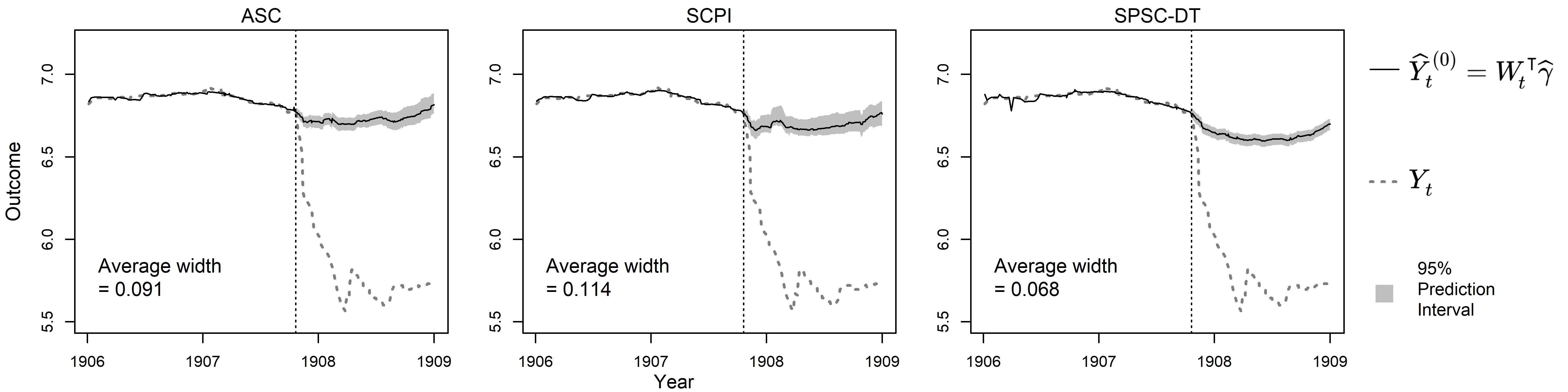
Additionally, for the sake of credibility, we conducted the following additional analysis for the application; the details can be found in Supplementary Material A.10. First, we studied the trend of the residuals, the difference between the observed outcome and synthetic control, over the pre-treatment time periods. We observed that the OLS-NoReg, SCPI, and SPSC-DT estimators produced residuals without a deterministic trend over time, while the other three estimators (OLS-Standard, ASC, SPSC-NoDT) showed the opposite behavior. Notably, the SPSC-DT estimator appears to satisfy the zero mean condition of Assumption 3.2, whereas the SPSC-NoDT estimator seems to violate this condition due to a non-zero deterministic trend over time. This again highlights the importance of accommodating time-varying components in the SPSC estimation procedure.
Next, we performed the following falsification study. We restricted the entire analysis to the pre-treatment period in which the causal effect is expected to be null. We artificially defined a financial panic time in late July 1907, which is roughly three months before the actual financial panic. This resulted in the lengths of the pre- and post-treatment periods equal to and , respectively. The proposed SPSC-NoDT and SPSC-DT estimators resulted in the placebo ATT estimates of and with 95% confidence intervals of and , respectively. The placebo ATT estimate obtained from the unconstrained OLS estimator was with a 95% confidence interval of . All 95% prediction intervals include the null, consistent with the expectation of no treatment effect in the placebo period. Lastly, the constrained OLS estimator (i.e., OLS-Standard), ASC estimator, and SCPI estimator produced placebo ATT estimates of , , and , respectively, which are also close to zero; however, corresponding statistical inference was not available for these estimators. Therefore, these results provide no evidence against validity of the estimators. In Supplementary Material A.10, we provide a trajectory of the synthetic controls along with 95% prediction intervals under the placebo treatment. Our findings indicate that the 95% prediction intervals from the SPSC-DT estimator support the null causal effect. However, the ASC and SCPI estimators occasionally fail to do so during certain time periods. Therefore, we conclude that the SPSC-DT estimator provides a more reliable framework for analyzing the impact of financial panic on the stock prices of the two trust companies.
6 Concluding Remarks
In this paper, we propose a novel SPSC approach in which the synthetic control is defined as a linear combination of donors’ outcomes whose conditional expectation matches the treatment-free potential outcome in both pre- and post-treatment periods. The model is analogous yet more general than measurement error models widely studied in standard measurement error literature. Under the framework, we establish the identification of a synthetic control, and provide an estimation strategy for the ATT. Furthermore, we introduce a method for inferring the treatment effect through pointwise prediction intervals, which remains valid even in the case of a short post-treatment period. We validate our methods through simulation studies and provide an application analyzing a real-world financial dataset related to the 1907 Panic.
We reiterate that the SPSC framework differs from existing synthetic control methods in its identifying assumptions and interpretation. It views the synthetic control as an error-prone outcome measurement, without the need for specifying a generative model for the outcome, whereas existing approaches treat it as the projection of the outcome onto the donor’s outcome space or the outcome itself. Despite these differences, both frameworks construct synthetic controls by optimally weighting donor units (according to their identifying assumptions), which are then used for treatment effect estimation. Additionally, like other synthetic control methods, the SPSC framework allows for time-varying confounders, as demonstrated in the generative models in Section 3.2.
While, as mentioned in Section 3.1, the SPSC framework may be viewed as a nonstandard form of instrumental variable approach, it is important to highlight key distinctions between the proposed SPSC approach and well-known instrumental variable approaches in dynamic panel data, such as in Anderson and Hsiao 1981 and Arellano and Bond 1991. In dynamic panel data models, endogeneity arises across different time periods, with the typical assumption that there is no within-time period endogeneity. As a result, these models use lagged variables as instruments to address cross-time endogeneity. In contrast, in the SPSC framework, endogeneity occurs within each time period, without specific assumptions about cross-time endogeneity. Consequently, the instrumental variable approach in this context operates within a single time period. We remark that, like the SPSC framework, many synthetic control models are agnostic about cross-time dependence structure; for example, the cross-time dependent structure of in the IFEM (2.2) is agnostic. A notable exception to this agnostic perspective is the “Instrumental variable-like SC estimator” proposed by Ferman and Pinto 2019, an earlier version of Ferman and Pinto 2021, which was developed in the presence of serial correlation in . Similar to estimators used in dynamic panel data models, it employs lagged variables as instruments.
As briefly mentioned in the introduction, the proposed SPSC framework has a connection to the single proxy control framework (Tchetgen Tchetgen 2013; Park et al. 2024) developed for i.i.d. data. In particular, Park et al. 2024 proposed an approach that relies on a so-called outcome bridge function, which is a (potentially nonlinear) function of outcome proxies. An important property of the outcome bridge function is that it is conditionally unbiased for the treatment-free potential outcome. Therefore, the proposed SPSC approach can be viewed as an adaptation of the outcome bridge function-based single proxy control approach to the synthetic control setting, where the outcome bridge function is known a priori to be a linear function of donors’ outcomes. In Supplementary Material B, we present a general SPSC framework, which is designed to accommodate nonparametric and nonlinear synthetic controls. Therefore, this framework obviates the over-reliance on a linear specification of synthetic controls in the literature and establishes a more direct connection with the outcome bridge function-based single proxy approach presented in Park et al. 2024. Notably, the general SPSC framework addresses underdeveloped areas of the synthetic control literature by allowing for various types of outcomes, including continuous, binary, count, or a combination of these.
In addition to the outcome bridge function-based approach, Park et al. 2024 introduced two other single proxy control approaches for i.i.d. sampling. One approach relies on propensity score weighting, eliminating the need for specifying an outcome bridge function. The second approach uses both the propensity score and the outcome bridge function and, more importantly, exhibits a doubly-robust property in that the treatment effect in view is identified if either propensity score or outcome bridge function, but not necessarily both, is correctly specified. Consequently, a promising direction for future research would be to develop new SPSC approaches by extending these single proxy methods to the synthetic control setting. Such new SPSC approaches can be viewed as complementing the doubly-robust proximal synthetic control approach (Qiu et al. 2024). However, such extensions pose significant challenges due to (i) a single treated unit with non-random treatment assignment, (ii) multiple heterogeneous untreated donor units; and (iii) serial correlation and heteroskedasticity due to the time series nature of the data. In particular, non-random treatment assignment undermines the conventional notion of the propensity score, rendering it undefined. Approaches for addressing these challenges and developing corresponding statistical methods will be considered elsewhere.
Appendix A Details of the Paper
A.1 Inconsistency of the Ordinary Least Squares Estimator
Following Ferman and Pinto 2021, we provide details on why synthetic controls obtained from the ordinary least squares (OLS) may be inconsistent. For simplicity, we consider an unconstrained case, in which equation (7) of the main paper reduces to:
| (7) |
For a fixed , the probability limit of as is given as follows:
| (27) |
where the second and third lines hold from (3) and (2.2) of the main paper, respectively, which are restated below:
and
| (3) |
The last line holds under the following additional assumptions on and as :
where is positive semidefinite. Clearly, is not the minimizer of (27) unless , i.e., a noiseless setting. Therefore, the OLS weights defined in (7) converge to the minimizer of as , which is different from the true synthetic control weights satisfying . This implies that the OLS estimator is inconsistent for unless .
A.2 Choice of the Regularization Parameter
We choose the regularization parameter based on leave-one-out cross-validation; see Algorithm 1 below.
A.3 A Heteroskedasticity and Autocorrelation Consistent Covariance Matrix Estimator
We provide details of a heteroskedasticity and autocorrelation consistent (HAC) covariance matrix estimator, which are obtained by following approaches of Newey and West 1987 and Andrews 1991. Let and be the GMM estimators used in Theorem 3.3 and the corresponding estimating function, respectively. Then, for a given bandwidth and a kernel function , a heteroskedasticity and autocorrelation consistent estimator of is given as
Popular choices for the kernel function are Bartlett and quadratic spectral functions, which are defined as follows:
- •
Bartlett kernel:
- •
Quadratic spectral kernel:
For these two kernel functions, the bandwidth parameter can be chosen based on the approximation to the first-order autoregressive model; see Algorithm 2 for details. We use the quadratic spectral kernel function for the simulation studies and the data analysis of the main paper.
A.4 Block Bootstrap
In this section, we provide a moving block bootstrap method (Kunsch 1989; Liu and Singh 1992) adapted to our setting. Algorithm 3 provides details of the block bootstrap implementation. We remark that other block bootstrap methods can be adopted with minor modifications; see Lahiri 1999 for examples of block bootstrap methods.
The choice of block length is critical to the performance of block bootstrap methods. The optimal choice of for minimizing mean square error is known to be . In the simulation studies in Section 4, we use the bandwidth of the Bartlett kernel function in Algorithm 2 of which the rate is . As discussed, this choice seems reasonable based on the simulation results reported in Section A.8.
A.5 Examples Where Assumption 3.2 Holds But Condition 3.1 Is Violated
We provide an example that violation of Condition 3.1 does not necessarily imply violation of Assumption 3.2. Consider the following interactive fixed effects model (IFEM):
| (28) |
Note that the model allows for non-stationarity behaviors, as can be time-varying. The model also allows for for , i.e., independent errors, where for is the components of . Therefore, for any , we find
Note that does not depend on for any where as depends on . Therefore, there is no satisfying Condition 3.1 when errors are independent, unless is zero.
However, one can still find such that Assumption 3.2 is satisfied despite independent errors, i.e., there exists a weight vector satisfying
Specifically, let be a vector that solves the following two equations:
| (29) | ||||
| (30) |
Again, note that for all when errors are independent.
From a property of joint normal distributions, we can represent the conditional distribution of given as follows:
Therefore, we find the joint distribution of is represented as follows:
where denotes a generic variance. This implies that the conditional distribution is given by
| (31) |
where the last line holds from (29) and (30). Therefore, we get almost surely, implying that Assumption 3.2 is satisfied with . Note that the synthetic control weight vector exists even when errors are independent and the outcomes are non-stationary.
Assumption 3.2 can be satisfied for non-continuous outcomes. To illustrate this, consider the following latent variable model for count data:
Note that can be non-stationary because is allowed to be time-varying.
Let be a vector that satisfies . Then, we find
Note that the fourth line holds from
| (32) |
Consequently, we find
Therefore, we can find a synthetic control bridge function .
A.6 Details on Accommodating Time-varying Components
We provide a rationale that accommodating time-varying components can improve the performance of the SPSC approach. Specifically, we consider the IFEM (28), where is assumed to lie within the space spanned by , i.e.,
This assumption is reasonable if is defined as a set of rich basis functions, such as polynomials, trigonometric functions, splines, or wavelets.
A.6.1 Using the Time-invariant Estimating Equation
Suppose that the synthetic control weights are estimated by the time-invariant pre-treatment estimating equation:
For simplicity, we choose . Then, it is straightforward to show that the regularized GMM estimator of is given by
where
From the law of large numbers, we find
Therefore, the limit of is , which is the minimum-norm solution of the equation . Therefore, satisfies
If for all , i.e., the mean of is time-invariant, we have
| (33) |
and
| (34) |
Therefore, satisfies (31), implying that it is a valid synthetic control satisfying Assumption 3.2. Therefore, can be used to obtain a consistent estimate for the ATT.
However, the solution in general does not satisfy (29) when is time-varying. This is because conditions (33) and (34) are not generally satisfied. Therefore, fails to satisfy (31). Therefore, the synthetic control converges to a invalid synthetic control that fails to satisfy Assumption 3.2, leading to an inconsistent estimate for the ATT.
A.6.2 Using the Time-varying Estimating Equation
Suppose that the synthetic control weights are estimated by the time-varying pre-treatment estimating equation:
where satisfies for . Note that . For simplicity, we choose . Then, it is straightforward to show that the regularized GMM estimator of is given by
where
Note that , which results in
From the law of large numbers, we find
Since , we have where
We can re-define so that is of full rank. Therefore, the limit of is , which is the minimum-norm solution of the equation . Therefore, satisfies
Consequently, we further obtain
| (35) |
and
| (36) |
Therefore, satisfies (31), implying that is a valid synthetic control satisfying Assumption 3.2. Therefore, can be used to obtain a consistent estimate for the ATT.
A.7 Extension: Covariate Adjustment
In practice, a rich collection of measured exogenous covariates may be available. One may want to incorporate these covariates in the synthetic control analysis because using these covariates may improve efficiency. In this Section, we provide details on the SPSC framework by incorporating measured covariates. Specifically, we denote -dimensional measured exogenous covariates for unit at time as ; we remind the readers that is the treated unit and are the untreated units. Let be the collection of all measured covariates of donors at time . To account for covariates, we modify Assumptions 3.1 and 3.2 as follows:
Assumption A.1 (Proxy & Existence of a Synthetic Control Bridge Function).
There exists a function satisfying
| (37) | ||||||
| (38) |
Theorem A.1.
Leveraging the result of the Theorem, estimation and inference of the ATT with covariate adjustment can be established, which is a straightforward extension of Section 3.4. Consider that the bridge function is linear as follows:
Following 3.4, we define the following estimating function:
| (40) | ||||
where is the collection of the observed data at time , is a -dimensional user-specified function of , and is a user-specified treatment effect function. A example for includes:
We allow to be smaller than . Let be the minimum-norm solution for .
We assume that the treatment effect function is chosen so that the associated error process is weakly dependent:
Assumption A.2 (Weakly Dependent Error in the Presence of Covariates).
Let be . Then, the error process satisfies Assumption 3.3, i.e., converges to 0 as .
We then establish the asymptotic normality of the regularized GMM estimators ; see the formal statement below:
Theorem A.2.
Suppose that Assumptions 2.1, 2.2, A.1, and A.2 hold, are unique, and Regularity Conditions in Section C.2 hold. Let be the regularized GMM estimators where the estimating function (40) is used, i.e.,
where is the empirical mean of the estimating function and is a user-specified symmetric, block-diagonal positive definite matrix. Then, as , we have
where
Here, is a symmetric positive-definite matrix satisfying .
Estimators of and can be similarly defined as in Section 3.4, thus we omit the details here.
A.8 Additional Simulation Studies
We restate the data generating process of the simulation studies in Section 4. The length of pre- and post-treatment periods were given by and the number of donors were given by .
First, for each , we independently generated 4-dimensional latent factors from , with being independent across time periods. For the mean vector , we considered the following four specifications for :
The latent factor loadings for , i.e., latent factor loadings of untreated units, were specified as follows:
The latent factor loading , i.e., latent factor loading of the treated unit, was specified from either one of the followings:
The errors were generated independently across time periods from where were chosen from one of the following three matrices with the corresponding values in (20):
With these generated variables, and at were generated as
We review the six approaches employed for the analysis:
-
(OLS-NoReg) OLS-based approach based on (8) with no regularization.
-
(OLS-Standard) The standard synthetic control approach proposed by Abadie et al. 2010; we used synth R-package (Abadie et al. 2011).
-
(ASC) The augmented synthetic control approach proposed by Ben-Michael et al. 2021; we used augsynth (Ben-Michael 2023) R-package.
-
(SCPI) The synthetic control prediction interval approach proposed by Cattaneo et al. 2021; we used scpi (Cattaneo et al. 2023) R-package.
-
(SPSC-NoDT) The single proxy synthetic control approach with no time-varying component; we used SPSC (Park 2024) R-package.
-
(SPSC-DT) The single proxy synthetic control approach with time-varying components SPSC (Park 2024) R-package.
For the two SPSC estimators, we set and, for SPSC-DT, we additionally set , 6-dimensional cubic B-spline bases functions.
We first estimated the ATT . Figures 4-7 summarize the empirical distribution of the estimators graphically. Each figure is drawn in the following format:
- •
The vertical segments represent 95% Monte Carlo confidence interval for each estimator obtained from 500 estimates.
- •
The dots represent the empirical mean of 500 estimates.
- •
The colors (light gray, gray, and black) and line types (solid and dashed) encode a corresponding estimator
- •
The shape of the dots encode the length of the pre-treatment period, respectively.
- •
The -axis represents the magnitude of bias.
We find that the results are similar to those in Figure 2 of the main paper. When is generated from (Non-simplex) and has non-zero mean, we find the OLS-Standard, ASC, and SCPI estimators appear to have significant magnitudes of biases even under a large sample size.


In Tables 4 and 5, we first present numerical summaries of the simulation studies considered in the main paper. Each table is written in the following format:
- •
Bias row shows the empirical bias of 500 estimates;
- •
ASE row shows the asymptotic standard error obtained from the sandwich variance estimator;
- •
BSE row shows the bootstrap standard error obtained from the approach in Section A.4 of the Supplementary Material;
- •
ESE row shows the standard deviation of 500 estimates;
- •
MSE row shows the mean squared error of 500 estimates;
- •
Cover (ASE) and Cover (BSE) show the empirical coverage rates of 95% confidence intervals based on the asymptotic and bootstrap standard errors, respectively;
- •
Bias, standard errors, and mean squared error are scaled by factors of 10, 10, and 100, respectively, for readability.
We remark that the results in Tables 4-7 are similar to those in Table 1 of the main text. In particular, when is generated from (Non-simplex) and has a non-zero mean, we find the OLS-Standard, ASC, and SCPI estimators yield significant magnitudes of biases even under a large sample size. Moreover, these biases are not negligible compared to the magnitude of the empirical standard errors. Consequently, we can deduce that the failure of the ASC and SCPI approaches to attain the nominal coverage rate can be attributed to the non-diminishing bias.
| Statistics | Estimators and | ||||||||||||||
| OLS-NoReg | OLS-Standard | ASC | SCPI | SPSC-NoDT | SPSC-DT | ||||||||||
| 100 | 500 | 100 | 500 | 100 | 500 | 100 | 500 | 100 | 500 | 100 | 500 | ||||
| No trend with no intercept | Simplex | Independent errors | Bias | 0.015 | 0.021 | -0.008 | 0.033 | 0.009 | 0.023 | 0.008 | 0.023 | 0.007 | 0.022 | 0.006 | 0.022 |
| ASE | 0.779 | 0.329 | - | - | - | - | - | - | 0.727 | 0.325 | 0.728 | 0.325 | |||
| BSE | 0.838 | 0.338 | - | - | - | - | - | - | 0.728 | 0.325 | 0.730 | 0.324 | |||
| ESE | 0.730 | 0.319 | 0.836 | 0.377 | 0.722 | 0.319 | 0.722 | 0.318 | 0.716 | 0.316 | 0.714 | 0.316 | |||
| MSE | 0.532 | 0.102 | 0.697 | 0.143 | 0.520 | 0.102 | 0.520 | 0.102 | 0.512 | 0.100 | 0.509 | 0.100 | |||
| Coverage (ASE) | 0.954 | 0.952 | - | - | - | - | - | - | 0.950 | 0.954 | 0.948 | 0.954 | |||
| Coverage (BSE) | 0.966 | 0.954 | - | - | - | - | - | - | 0.946 | 0.950 | 0.946 | 0.948 | |||
| Correlated errors | Bias | 0.010 | 0.006 | -0.018 | 0.022 | 0.010 | 0.006 | 0.009 | 0.006 | 0.014 | 0.004 | 0.015 | 0.004 | ||
| ASE | 0.534 | 0.237 | - | - | - | - | - | - | 0.533 | 0.238 | 0.533 | 0.238 | |||
| BSE | 0.551 | 0.241 | - | - | - | - | - | - | 0.529 | 0.237 | 0.529 | 0.237 | |||
| ESE | 0.568 | 0.242 | 0.688 | 0.298 | 0.565 | 0.243 | 0.565 | 0.243 | 0.565 | 0.243 | 0.564 | 0.243 | |||
| MSE | 0.322 | 0.059 | 0.473 | 0.089 | 0.319 | 0.059 | 0.319 | 0.059 | 0.318 | 0.059 | 0.318 | 0.059 | |||
| Coverage (ASE) | 0.940 | 0.944 | - | - | - | - | - | - | 0.934 | 0.954 | 0.936 | 0.954 | |||
| Coverage (BSE) | 0.940 | 0.952 | - | - | - | - | - | - | 0.922 | 0.946 | 0.936 | 0.946 | |||
| No error | Bias | -0.016 | 0.012 | -0.008 | 0.007 | -0.021 | 0.011 | -0.021 | 0.011 | -0.020 | 0.011 | -0.020 | 0.011 | ||
| ASE | 0.527 | 0.234 | - | - | - | - | - | - | 0.525 | 0.234 | 0.525 | 0.234 | |||
| BSE | 0.542 | 0.238 | - | - | - | - | - | - | 0.523 | 0.233 | 0.522 | 0.233 | |||
| ESE | 0.541 | 0.231 | 0.626 | 0.275 | 0.539 | 0.229 | 0.539 | 0.229 | 0.536 | 0.231 | 0.536 | 0.231 | |||
| MSE | 0.292 | 0.053 | 0.391 | 0.076 | 0.290 | 0.052 | 0.290 | 0.052 | 0.287 | 0.053 | 0.287 | 0.053 | |||
| Coverage (ASE) | 0.944 | 0.954 | - | - | - | - | - | - | 0.948 | 0.954 | 0.948 | 0.952 | |||
| Coverage (BSE) | 0.946 | 0.956 | - | - | - | - | - | - | 0.946 | 0.948 | 0.948 | 0.950 | |||
| Non-simplex | Independent errors | Bias | 0.022 | -0.009 | 0.042 | 0.000 | 0.028 | -0.010 | 0.032 | -0.011 | 0.031 | -0.009 | 0.027 | -0.008 | |
| ASE | 0.895 | 0.373 | - | - | - | - | - | - | 0.837 | 0.373 | 0.837 | 0.372 | |||
| BSE | 0.970 | 0.383 | - | - | - | - | - | - | 0.845 | 0.374 | 0.839 | 0.372 | |||
| ESE | 0.920 | 0.373 | 1.248 | 0.506 | 0.905 | 0.387 | 0.918 | 0.392 | 0.888 | 0.371 | 0.889 | 0.371 | |||
| MSE | 0.845 | 0.139 | 1.556 | 0.256 | 0.817 | 0.150 | 0.841 | 0.154 | 0.788 | 0.137 | 0.789 | 0.138 | |||
| Coverage (ASE) | 0.950 | 0.958 | - | - | - | - | - | - | 0.932 | 0.956 | 0.934 | 0.956 | |||
| Coverage (BSE) | 0.962 | 0.962 | - | - | - | - | - | - | 0.934 | 0.958 | 0.930 | 0.960 | |||
| Correlated errors | Bias | -0.046 | -0.023 | 0.022 | -0.024 | -0.037 | -0.025 | -0.031 | -0.028 | -0.028 | -0.017 | -0.026 | -0.019 | ||
| ASE | 0.630 | 0.274 | - | - | - | - | - | - | 0.660 | 0.295 | 0.667 | 0.297 | |||
| BSE | 0.668 | 0.280 | - | - | - | - | - | - | 0.665 | 0.295 | 0.679 | 0.300 | |||
| ESE | 0.619 | 0.278 | 1.049 | 0.497 | 0.630 | 0.277 | 0.644 | 0.284 | 0.670 | 0.293 | 0.666 | 0.296 | |||
| MSE | 0.385 | 0.077 | 1.098 | 0.247 | 0.398 | 0.077 | 0.415 | 0.081 | 0.449 | 0.086 | 0.443 | 0.088 | |||
| Coverage (ASE) | 0.948 | 0.942 | - | - | - | - | - | - | 0.938 | 0.944 | 0.936 | 0.940 | |||
| Coverage (BSE) | 0.960 | 0.948 | - | - | - | - | - | - | 0.940 | 0.948 | 0.936 | 0.946 | |||
| No error | Bias | -0.017 | 0.019 | -0.038 | 0.003 | -0.009 | 0.016 | -0.009 | 0.015 | -0.009 | 0.018 | -0.011 | 0.017 | ||
| ASE | 0.693 | 0.293 | - | - | - | - | - | - | 0.665 | 0.293 | 0.665 | 0.293 | |||
| BSE | 0.737 | 0.301 | - | - | - | - | - | - | 0.673 | 0.292 | 0.670 | 0.292 | |||
| ESE | 0.712 | 0.290 | 1.023 | 0.437 | 0.717 | 0.303 | 0.730 | 0.311 | 0.695 | 0.291 | 0.699 | 0.291 | |||
| MSE | 0.506 | 0.084 | 1.045 | 0.191 | 0.513 | 0.092 | 0.532 | 0.097 | 0.482 | 0.085 | 0.488 | 0.085 | |||
| Coverage (ASE) | 0.936 | 0.954 | - | - | - | - | - | - | 0.936 | 0.946 | 0.932 | 0.948 | |||
| Coverage (BSE) | 0.952 | 0.958 | - | - | - | - | - | - | 0.936 | 0.948 | 0.930 | 0.948 | |||
| Statistics | Estimators and | ||||||||||||||
| OLS-NoReg | OLS-Standard | ASC | SCPI | SPSC-NoDT | SPSC-DT | ||||||||||
| 100 | 500 | 100 | 500 | 100 | 500 | 100 | 500 | 100 | 500 | 100 | 500 | ||||
| No trend with intercept | Simplex | Independent errors | Bias | 0.075 | 0.073 | 0.026 | 0.001 | -0.141 | -0.107 | -0.142 | -0.107 | -0.683 | -0.925 | 0.008 | 0.005 |
| ASE | 0.916 | 0.399 | - | - | - | - | - | - | 0.924 | 0.418 | 0.886 | 0.399 | |||
| BSE | 1.002 | 0.411 | - | - | - | - | - | - | 0.982 | 0.443 | 0.898 | 0.400 | |||
| ESE | 0.930 | 0.390 | 1.022 | 0.467 | 0.909 | 0.387 | 0.907 | 0.388 | 1.115 | 0.466 | 0.921 | 0.390 | |||
| MSE | 0.868 | 0.157 | 1.042 | 0.217 | 0.844 | 0.161 | 0.841 | 0.162 | 1.708 | 1.072 | 0.847 | 0.152 | |||
| Coverage (ASE) | 0.944 | 0.940 | - | - | - | - | - | - | 0.842 | 0.400 | 0.938 | 0.956 | |||
| Coverage (BSE) | 0.960 | 0.954 | - | - | - | - | - | - | 0.854 | 0.436 | 0.948 | 0.960 | |||
| Correlated errors | Bias | -0.010 | -0.012 | 0.016 | 0.003 | -0.034 | -0.027 | -0.035 | -0.027 | -0.399 | -0.335 | -0.026 | -0.022 | ||
| ASE | 0.554 | 0.248 | - | - | - | - | - | - | 0.742 | 0.334 | 0.556 | 0.251 | |||
| BSE | 0.577 | 0.252 | - | - | - | - | - | - | 0.763 | 0.345 | 0.554 | 0.251 | |||
| ESE | 0.557 | 0.237 | 0.795 | 0.358 | 0.552 | 0.237 | 0.552 | 0.237 | 0.783 | 0.328 | 0.558 | 0.240 | |||
| MSE | 0.310 | 0.056 | 0.631 | 0.128 | 0.306 | 0.057 | 0.305 | 0.057 | 0.772 | 0.220 | 0.311 | 0.058 | |||
| Coverage (ASE) | 0.950 | 0.950 | - | - | - | - | - | - | 0.902 | 0.824 | 0.954 | 0.944 | |||
| Coverage (BSE) | 0.958 | 0.954 | - | - | - | - | - | - | 0.898 | 0.842 | 0.950 | 0.950 | |||
| No error | Bias | 0.113 | 0.079 | 0.098 | 0.004 | -0.063 | -0.087 | -0.064 | -0.087 | -0.247 | -0.401 | 0.042 | 0.008 | ||
| ASE | 0.544 | 0.244 | - | - | - | - | - | - | 0.679 | 0.305 | 0.544 | 0.244 | |||
| BSE | 0.566 | 0.248 | - | - | - | - | - | - | 0.678 | 0.305 | 0.542 | 0.244 | |||
| ESE | 0.543 | 0.249 | 0.732 | 0.344 | 0.547 | 0.254 | 0.547 | 0.254 | 0.705 | 0.314 | 0.539 | 0.249 | |||
| MSE | 0.307 | 0.068 | 0.545 | 0.118 | 0.302 | 0.072 | 0.302 | 0.072 | 0.557 | 0.259 | 0.292 | 0.062 | |||
| Coverage (ASE) | 0.942 | 0.944 | - | - | - | - | - | - | 0.932 | 0.732 | 0.954 | 0.956 | |||
| Coverage (BSE) | 0.950 | 0.948 | - | - | - | - | - | - | 0.928 | 0.736 | 0.952 | 0.958 | |||
| Non-simplex | Independent errors | Bias | 0.381 | 0.351 | 7.010 | 6.987 | 2.540 | 1.375 | 7.358 | 7.308 | -0.267 | -0.344 | 0.036 | 0.004 | |
| ASE | 1.104 | 0.474 | - | - | - | - | - | - | 1.282 | 0.575 | 1.058 | 0.476 | |||
| BSE | 1.223 | 0.489 | - | - | - | - | - | - | 1.321 | 0.596 | 1.086 | 0.483 | |||
| ESE | 1.141 | 0.474 | 0.939 | 0.438 | 1.357 | 0.564 | 0.935 | 0.448 | 1.302 | 0.571 | 1.090 | 0.485 | |||
| MSE | 1.444 | 0.347 | 50.020 | 49.005 | 8.289 | 2.208 | 55.011 | 53.601 | 1.762 | 0.443 | 1.187 | 0.235 | |||
| Coverage (ASE) | 0.920 | 0.884 | - | - | - | - | - | - | 0.950 | 0.914 | 0.942 | 0.930 | |||
| Coverage (BSE) | 0.948 | 0.894 | - | - | - | - | - | - | 0.946 | 0.922 | 0.948 | 0.936 | |||
| Correlated errors | Bias | 0.218 | 0.249 | 7.019 | 7.012 | 0.763 | 0.406 | 7.018 | 7.011 | 0.085 | 0.276 | 0.004 | 0.020 | ||
| ASE | 0.728 | 0.317 | - | - | - | - | - | - | 1.084 | 0.485 | 0.827 | 0.372 | |||
| BSE | 0.784 | 0.325 | - | - | - | - | - | - | 1.098 | 0.495 | 0.849 | 0.384 | |||
| ESE | 0.749 | 0.321 | 0.680 | 0.286 | 0.880 | 0.324 | 0.680 | 0.286 | 1.237 | 0.477 | 0.816 | 0.362 | |||
| MSE | 0.607 | 0.165 | 49.721 | 49.244 | 1.354 | 0.270 | 49.718 | 49.241 | 1.535 | 0.303 | 0.665 | 0.131 | |||
| Coverage (ASE) | 0.944 | 0.854 | - | - | - | - | - | - | 0.892 | 0.926 | 0.956 | 0.948 | |||
| Coverage (BSE) | 0.958 | 0.874 | - | - | - | - | - | - | 0.896 | 0.940 | 0.954 | 0.962 | |||
| No error | Bias | 0.367 | 0.340 | 7.051 | 6.971 | 1.826 | 1.216 | 7.391 | 7.294 | 0.205 | 0.251 | 0.036 | -0.002 | ||
| ASE | 0.815 | 0.353 | - | - | - | - | - | - | 1.103 | 0.495 | 0.797 | 0.356 | |||
| BSE | 0.886 | 0.363 | - | - | - | - | - | - | 1.122 | 0.509 | 0.813 | 0.361 | |||
| ESE | 0.840 | 0.326 | 0.788 | 0.345 | 0.975 | 0.387 | 0.797 | 0.350 | 1.244 | 0.484 | 0.811 | 0.331 | |||
| MSE | 0.839 | 0.222 | 50.338 | 48.716 | 4.284 | 1.627 | 55.260 | 53.321 | 1.586 | 0.297 | 0.658 | 0.109 | |||
| Coverage (ASE) | 0.922 | 0.856 | - | - | - | - | - | - | 0.916 | 0.930 | 0.942 | 0.966 | |||
| Coverage (BSE) | 0.936 | 0.868 | - | - | - | - | - | - | 0.920 | 0.948 | 0.956 | 0.968 | |||
| Statistics | Estimators and | ||||||||||||||
| OLS-NoReg | OLS-Standard | ASC | SCPI | SPSC-NoDT | SPSC-DT | ||||||||||
| 100 | 500 | 100 | 500 | 100 | 500 | 100 | 500 | 100 | 500 | 100 | 500 | ||||
| Linear trend with no intercept | Simplex | Independent errors | Bias | 0.323 | 0.274 | 0.127 | -0.021 | -0.498 | -0.420 | -0.507 | -0.426 | -1.212 | -0.971 | 0.071 | 0.006 |
| ASE | 1.425 | 0.636 | - | - | - | - | - | - | 1.225 | 0.552 | 1.429 | 0.649 | |||
| BSE | 1.628 | 0.658 | - | - | - | - | - | - | 1.794 | 0.825 | 1.534 | 0.683 | |||
| ESE | 1.482 | 0.598 | 2.061 | 0.900 | 1.361 | 0.582 | 1.355 | 0.582 | 2.885 | 2.871 | 1.518 | 0.645 | |||
| MSE | 2.298 | 0.432 | 4.254 | 0.808 | 2.096 | 0.515 | 2.089 | 0.520 | 9.779 | 9.168 | 2.304 | 0.415 | |||
| Coverage (ASE) | 0.926 | 0.946 | - | - | - | - | - | - | 0.438 | 0.034 | 0.946 | 0.952 | |||
| Coverage (BSE) | 0.960 | 0.954 | - | - | - | - | - | - | 0.668 | 0.156 | 0.962 | 0.968 | |||
| Correlated errors | Bias | 0.006 | -0.009 | 0.131 | 0.017 | -0.105 | -0.074 | -0.110 | -0.076 | -1.945 | -1.347 | -0.079 | -0.088 | ||
| ASE | 0.654 | 0.294 | - | - | - | - | - | - | 0.902 | 0.405 | 0.662 | 0.301 | |||
| BSE | 0.703 | 0.302 | - | - | - | - | - | - | 0.978 | 0.468 | 0.711 | 0.320 | |||
| ESE | 0.701 | 0.289 | 1.468 | 0.697 | 0.663 | 0.285 | 0.662 | 0.285 | 1.352 | 0.686 | 0.704 | 0.332 | |||
| MSE | 0.491 | 0.084 | 2.167 | 0.486 | 0.450 | 0.087 | 0.450 | 0.087 | 5.606 | 2.284 | 0.500 | 0.118 | |||
| Coverage (ASE) | 0.922 | 0.950 | - | - | - | - | - | - | 0.470 | 0.176 | 0.922 | 0.926 | |||
| Coverage (BSE) | 0.948 | 0.958 | - | - | - | - | - | - | 0.518 | 0.260 | 0.948 | 0.942 | |||
| No error | Bias | 0.280 | 0.288 | 0.105 | 0.036 | -0.373 | -0.321 | -0.376 | -0.321 | -1.154 | -1.364 | 0.028 | 0.016 | ||
| ASE | 0.635 | 0.285 | - | - | - | - | - | - | 0.858 | 0.388 | 0.642 | 0.288 | |||
| BSE | 0.683 | 0.292 | - | - | - | - | - | - | 0.851 | 0.374 | 0.664 | 0.299 | |||
| ESE | 0.671 | 0.286 | 1.391 | 0.633 | 0.662 | 0.293 | 0.663 | 0.294 | 1.040 | 0.383 | 0.705 | 0.309 | |||
| MSE | 0.528 | 0.165 | 1.941 | 0.401 | 0.577 | 0.189 | 0.580 | 0.189 | 2.411 | 2.006 | 0.497 | 0.095 | |||
| Coverage (ASE) | 0.906 | 0.820 | - | - | - | - | - | - | 0.648 | 0.062 | 0.920 | 0.930 | |||
| Coverage (BSE) | 0.930 | 0.832 | - | - | - | - | - | - | 0.642 | 0.054 | 0.926 | 0.940 | |||
| Non-simplex | Independent errors | Bias | 1.302 | 1.366 | 10.695 | 10.506 | 8.262 | 5.699 | 11.927 | 11.849 | -1.421 | -1.612 | 0.069 | 0.083 | |
| ASE | 1.760 | 0.789 | - | - | - | - | - | - | 1.851 | 0.836 | 1.795 | 0.814 | |||
| BSE | 2.021 | 0.816 | - | - | - | - | - | - | 2.242 | 0.991 | 1.941 | 0.865 | |||
| ESE | 1.823 | 0.766 | 1.159 | 0.406 | 1.702 | 0.949 | 0.962 | 0.433 | 2.084 | 0.973 | 1.938 | 0.847 | |||
| MSE | 5.013 | 2.451 | 115.724 | 110.539 | 71.157 | 33.373 | 143.178 | 140.580 | 6.357 | 3.543 | 3.753 | 0.723 | |||
| Coverage (ASE) | 0.872 | 0.582 | - | - | - | - | - | - | 0.840 | 0.486 | 0.928 | 0.940 | |||
| Coverage (BSE) | 0.934 | 0.610 | - | - | - | - | - | - | 0.914 | 0.604 | 0.942 | 0.958 | |||
| Correlated errors | Bias | 1.002 | 0.998 | 10.518 | 10.508 | 2.675 | 1.589 | 10.521 | 10.507 | -0.096 | 0.789 | 0.219 | 0.098 | ||
| ASE | 1.033 | 0.464 | - | - | - | - | - | - | 1.484 | 0.660 | 1.330 | 0.614 | |||
| BSE | 1.162 | 0.477 | - | - | - | - | - | - | 1.655 | 0.766 | 1.424 | 0.650 | |||
| ESE | 1.088 | 0.438 | 0.642 | 0.286 | 1.538 | 0.520 | 0.644 | 0.286 | 2.158 | 0.877 | 1.345 | 0.584 | |||
| MSE | 2.185 | 1.187 | 111.044 | 110.490 | 9.519 | 2.794 | 111.110 | 110.482 | 4.656 | 1.391 | 1.853 | 0.350 | |||
| Coverage (ASE) | 0.824 | 0.434 | - | - | - | - | - | - | 0.796 | 0.716 | 0.934 | 0.960 | |||
| Coverage (BSE) | 0.864 | 0.440 | - | - | - | - | - | - | 0.822 | 0.792 | 0.948 | 0.968 | |||
| No error | Bias | 1.430 | 1.373 | 10.681 | 10.492 | 6.747 | 4.740 | 11.887 | 11.833 | 0.163 | 0.670 | 0.199 | 0.127 | ||
| ASE | 1.221 | 0.544 | - | - | - | - | - | - | 1.562 | 0.696 | 1.253 | 0.563 | |||
| BSE | 1.383 | 0.561 | - | - | - | - | - | - | 1.830 | 0.841 | 1.353 | 0.598 | |||
| ESE | 1.274 | 0.560 | 1.095 | 0.368 | 1.671 | 0.649 | 0.805 | 0.345 | 2.253 | 0.788 | 1.306 | 0.613 | |||
| MSE | 3.663 | 2.197 | 115.286 | 110.212 | 48.307 | 22.885 | 141.959 | 140.136 | 5.093 | 1.069 | 1.742 | 0.391 | |||
| Coverage (ASE) | 0.758 | 0.300 | - | - | - | - | - | - | 0.832 | 0.822 | 0.930 | 0.918 | |||
| Coverage (BSE) | 0.820 | 0.328 | - | - | - | - | - | - | 0.880 | 0.898 | 0.942 | 0.928 | |||
| Statistics | Estimators and | ||||||||||||||
| OLS-NoReg | OLS-Standard | ASC | SCPI | SPSC-NoDT | SPSC-DT | ||||||||||
| 100 | 500 | 100 | 500 | 100 | 500 | 100 | 500 | 100 | 500 | 100 | 500 | ||||
| Linear trend with intercept | Simplex | Independent errors | Bias | 0.091 | 0.079 | 0.012 | 0.001 | -0.173 | -0.134 | -0.169 | -0.133 | -0.547 | -0.621 | 0.020 | -0.005 |
| ASE | 1.131 | 0.498 | - | - | - | - | - | - | 1.183 | 0.535 | 1.107 | 0.502 | |||
| BSE | 1.261 | 0.514 | - | - | - | - | - | - | 1.269 | 0.576 | 1.134 | 0.506 | |||
| ESE | 1.198 | 0.494 | 1.345 | 0.606 | 1.152 | 0.495 | 1.152 | 0.495 | 1.341 | 0.591 | 1.147 | 0.507 | |||
| MSE | 1.441 | 0.249 | 1.806 | 0.367 | 1.355 | 0.263 | 1.353 | 0.262 | 2.095 | 0.734 | 1.313 | 0.257 | |||
| Coverage (ASE) | 0.928 | 0.942 | - | - | - | - | - | - | 0.886 | 0.758 | 0.930 | 0.958 | |||
| Coverage (BSE) | 0.948 | 0.958 | - | - | - | - | - | - | 0.908 | 0.798 | 0.938 | 0.950 | |||
| Correlated errors | Bias | -0.026 | 0.015 | -0.002 | -0.001 | -0.066 | -0.006 | -0.064 | -0.005 | -0.697 | -0.450 | -0.035 | 0.012 | ||
| ASE | 0.594 | 0.265 | - | - | - | - | - | - | 0.944 | 0.424 | 0.600 | 0.271 | |||
| BSE | 0.626 | 0.271 | - | - | - | - | - | - | 0.969 | 0.441 | 0.604 | 0.272 | |||
| ESE | 0.612 | 0.259 | 1.028 | 0.467 | 0.594 | 0.258 | 0.594 | 0.258 | 1.115 | 0.723 | 0.619 | 0.265 | |||
| MSE | 0.374 | 0.067 | 1.054 | 0.218 | 0.357 | 0.066 | 0.357 | 0.066 | 1.726 | 0.724 | 0.384 | 0.070 | |||
| Coverage (ASE) | 0.948 | 0.954 | - | - | - | - | - | - | 0.830 | 0.626 | 0.936 | 0.954 | |||
| Coverage (BSE) | 0.956 | 0.954 | - | - | - | - | - | - | 0.828 | 0.642 | 0.940 | 0.950 | |||
| No error | Bias | 0.085 | 0.089 | 0.025 | 0.021 | -0.121 | -0.098 | -0.120 | -0.099 | -0.309 | -0.322 | 0.002 | 0.007 | ||
| ASE | 0.580 | 0.260 | - | - | - | - | - | - | 0.826 | 0.372 | 0.582 | 0.261 | |||
| BSE | 0.611 | 0.265 | - | - | - | - | - | - | 0.830 | 0.373 | 0.587 | 0.261 | |||
| ESE | 0.583 | 0.266 | 0.925 | 0.419 | 0.603 | 0.273 | 0.603 | 0.273 | 0.844 | 0.388 | 0.578 | 0.266 | |||
| MSE | 0.347 | 0.078 | 0.855 | 0.176 | 0.378 | 0.084 | 0.377 | 0.084 | 0.806 | 0.254 | 0.333 | 0.070 | |||
| Coverage (ASE) | 0.952 | 0.946 | - | - | - | - | - | - | 0.924 | 0.858 | 0.956 | 0.956 | |||
| Coverage (BSE) | 0.970 | 0.952 | - | - | - | - | - | - | 0.922 | 0.850 | 0.954 | 0.942 | |||
| Non-simplex | Independent errors | Bias | 0.383 | 0.424 | 17.500 | 17.531 | 2.818 | 1.497 | 17.517 | 17.530 | 0.256 | 0.339 | -0.009 | 0.040 | |
| ASE | 1.394 | 0.608 | - | - | - | - | - | - | 1.724 | 0.775 | 1.362 | 0.613 | |||
| BSE | 1.571 | 0.629 | - | - | - | - | - | - | 1.798 | 0.810 | 1.416 | 0.621 | |||
| ESE | 1.470 | 0.627 | 0.909 | 0.450 | 1.798 | 0.708 | 0.911 | 0.450 | 1.789 | 0.799 | 1.399 | 0.638 | |||
| MSE | 2.303 | 0.572 | 307.074 | 307.536 | 11.169 | 2.743 | 307.689 | 307.513 | 3.260 | 0.751 | 1.953 | 0.407 | |||
| Coverage (ASE) | 0.926 | 0.886 | - | - | - | - | - | - | 0.934 | 0.928 | 0.934 | 0.954 | |||
| Coverage (BSE) | 0.962 | 0.894 | - | - | - | - | - | - | 0.938 | 0.934 | 0.946 | 0.952 | |||
| Correlated errors | Bias | 0.287 | 0.247 | 17.548 | 17.488 | 1.028 | 0.440 | 17.547 | 17.487 | -0.427 | -0.738 | 0.023 | -0.018 | ||
| ASE | 0.862 | 0.378 | - | - | - | - | - | - | 1.472 | 0.662 | 1.020 | 0.459 | |||
| BSE | 0.950 | 0.388 | - | - | - | - | - | - | 1.475 | 0.665 | 1.067 | 0.478 | |||
| ESE | 0.906 | 0.382 | 0.661 | 0.300 | 1.138 | 0.394 | 0.661 | 0.300 | 1.696 | 0.806 | 1.012 | 0.455 | |||
| MSE | 0.902 | 0.207 | 308.369 | 305.912 | 2.349 | 0.349 | 308.345 | 305.890 | 3.052 | 1.193 | 1.022 | 0.207 | |||
| Coverage (ASE) | 0.924 | 0.882 | - | - | - | - | - | - | 0.902 | 0.734 | 0.934 | 0.946 | |||
| Coverage (BSE) | 0.948 | 0.888 | - | - | - | - | - | - | 0.906 | 0.736 | 0.940 | 0.954 | |||
| No error | Bias | 0.385 | 0.388 | 17.573 | 17.520 | 1.884 | 1.388 | 17.575 | 17.519 | -0.421 | -0.506 | 0.010 | 0.014 | ||
| ASE | 0.983 | 0.435 | - | - | - | - | - | - | 1.494 | 0.674 | 0.979 | 0.439 | |||
| BSE | 1.092 | 0.449 | - | - | - | - | - | - | 1.515 | 0.678 | 1.012 | 0.446 | |||
| ESE | 1.091 | 0.432 | 0.797 | 0.360 | 1.316 | 0.508 | 0.798 | 0.360 | 1.800 | 1.006 | 1.080 | 0.439 | |||
| MSE | 1.336 | 0.337 | 309.455 | 307.081 | 5.278 | 2.185 | 309.528 | 307.059 | 3.412 | 1.265 | 1.164 | 0.192 | |||
| Coverage (ASE) | 0.900 | 0.846 | - | - | - | - | - | - | 0.880 | 0.750 | 0.924 | 0.960 | |||
| Coverage (BSE) | 0.932 | 0.866 | - | - | - | - | - | - | 0.882 | 0.744 | 0.936 | 0.962 | |||
We report the performance of conformal inference in Section 3.5 of the main paper under the simulation scenarios in Section 4 of the main paper. First, we obtain the pointwise 95% pointwise prediction interval for the random treatment effect at 10 post-treatment times , which are .
As competing methods, we construct 95% pointwise prediction intervals using the ASC and SCPI approaches. For the ASC approach, we use the conformal approach to construct prediction intervals, which is the default option employed in augsynth package. For the SCPI approach, we use the prediction interval estimating out-of-sample uncertainty with sub-Gaussian bounds, which is stored in CI.all.gaussian object of a scpi output; see below for an example R-code:
-
scpi.est scpi::scpi(SCD) # SCD is a scdata object
-
scpi.PI scpi.est$inference.results$CI.all.gaussian
For each simulation repetition and each method, we calculate where is a 95% prediction interval obtained from each method, i.e., the indicator of whether a 95% prediction interval at obtained from each method includes the random treatment effect. Ideally, the average of these indicators across simulation repetitions (i.e., the empirical coverage rate of 95% prediction intervals) should be close to the nominal coverage rate of 0.95.
Table 8 shows the empirical coverage rates obtained from 500 repetitions for each simulation scenario. We find that the conformal inference approach for the SPSC achieves the nominal coverage rate across all simulation scenarios in general. However, we find that the ASC approach fails to do so for all reported scenarios. Likewise, the SCPI approach appears to struggle to attain the desired nominal coverage rate, especially when the latent factor has a trend. Next, we calculate the average length of the 95% prediction intervals for across 500 repetitions. The table also shows the average lengths of the prediction intervals. We find that the length of the prediction intervals decreases as the length of the pre-treatment periods increases. Notably, the SPSC-DT approach consistently yields prediction intervals that are not only comparable in length but often the shortest when compared to other estimators across all scenarios. In particular, the SPSC-DT estimator outperforms the others in terms of coverage and length, particularly when a linear trend is present. These findings demonstrate that the proposed conformal inference method for the SPSC framework is robust and broadly applicable, regardless of the data generating process.
| Statistics | Estimators and | ||||||||||
| ASC | SCPI | SPSC-NoDT | SPSC-DT | ||||||||
| 100 | 500 | 100 | 500 | 100 | 500 | 100 | 500 | ||||
| No trend with no intercept | Simplex | Independent errors | Coverage | 0.925 | 0.918 | 0.907 | 0.939 | 0.963 | 0.954 | 0.963 | 0.954 |
| Length | 2.009 | 1.850 | 2.034 | 2.036 | 2.249 | 2.055 | 2.244 | 2.054 | |||
| Correlated errors | Coverage | 0.691 | 0.567 | 0.972 | 0.954 | 0.959 | 0.950 | 0.960 | 0.950 | ||
| Length | 0.423 | 0.283 | 0.872 | 0.706 | 0.755 | 0.696 | 0.766 | 0.696 | |||
| No error | Coverage | 0.714 | 0.581 | 0.986 | 0.961 | 0.959 | 0.948 | 0.960 | 0.948 | ||
| Length | 0.465 | 0.305 | 0.951 | 0.680 | 0.675 | 0.610 | 0.681 | 0.610 | |||
| Non-simplex | Independent errors | Coverage | 0.933 | 0.925 | 0.935 | 0.912 | 0.959 | 0.948 | 0.961 | 0.948 | |
| Length | 2.597 | 2.459 | 2.848 | 2.407 | 2.839 | 2.556 | 2.824 | 2.554 | |||
| Correlated errors | Coverage | 0.904 | 0.906 | 0.925 | 0.913 | 0.962 | 0.952 | 0.963 | 0.953 | ||
| Length | 1.326 | 1.229 | 1.440 | 1.255 | 1.859 | 1.701 | 1.935 | 1.699 | |||
| No error | Coverage | 0.922 | 0.910 | 0.938 | 0.925 | 0.964 | 0.951 | 0.964 | 0.953 | ||
| Length | 1.704 | 1.608 | 1.978 | 1.648 | 1.852 | 1.668 | 1.856 | 1.670 | |||
| No trend with intercept | Simplex | Independent errors | Coverage | 0.921 | 0.917 | 0.911 | 0.940 | 0.962 | 0.953 | 0.959 | 0.951 |
| Length | 1.998 | 1.861 | 2.068 | 2.069 | 2.599 | 2.410 | 2.245 | 2.061 | |||
| Correlated errors | Coverage | 0.674 | 0.580 | 0.969 | 0.958 | 0.962 | 0.955 | 0.961 | 0.948 | ||
| Length | 0.410 | 0.286 | 0.868 | 0.704 | 1.782 | 1.653 | 0.762 | 0.700 | |||
| No error | Coverage | 0.735 | 0.603 | 0.985 | 0.954 | 0.953 | 0.954 | 0.968 | 0.946 | ||
| Length | 0.489 | 0.324 | 0.935 | 0.666 | 1.469 | 1.366 | 0.693 | 0.618 | |||
| Non-simplex | Independent errors | Coverage | 0.927 | 0.921 | 0.898 | 0.877 | 0.960 | 0.947 | 0.958 | 0.946 | |
| Length | 3.064 | 2.746 | 2.741 | 2.410 | 3.778 | 3.511 | 2.887 | 2.638 | |||
| Correlated errors | Coverage | 0.911 | 0.907 | 0.893 | 0.883 | 0.965 | 0.953 | 0.967 | 0.953 | ||
| Length | 1.435 | 1.266 | 1.420 | 1.278 | 3.043 | 2.831 | 2.181 | 1.813 | |||
| No error | Coverage | 0.917 | 0.918 | 0.908 | 0.890 | 0.964 | 0.947 | 0.967 | 0.950 | ||
| Length | 2.198 | 1.958 | 2.046 | 1.751 | 3.130 | 2.901 | 1.968 | 1.744 | |||
| Linear trend with no intercept | Simplex | Independent errors | Coverage | 0.934 | 0.915 | 0.926 | 0.951 | 0.950 | 0.928 | 0.962 | 0.941 |
| Length | 2.100 | 1.879 | 2.372 | 2.252 | 2.675 | 2.376 | 2.288 | 2.074 | |||
| Correlated errors | Coverage | 0.744 | 0.593 | 0.985 | 0.969 | 0.919 | 0.935 | 0.959 | 0.949 | ||
| Length | 0.490 | 0.300 | 1.028 | 0.767 | 1.603 | 1.421 | 0.774 | 0.700 | |||
| No error | Coverage | 0.780 | 0.620 | 0.991 | 0.973 | 0.941 | 0.930 | 0.961 | 0.955 | ||
| Length | 0.553 | 0.353 | 1.063 | 0.725 | 1.392 | 1.225 | 0.704 | 0.620 | |||
| Non-simplex | Independent errors | Coverage | 0.795 | 0.846 | 0.938 | 0.889 | 0.959 | 0.944 | 0.962 | 0.949 | |
| Length | 2.969 | 2.719 | 3.223 | 2.646 | 3.755 | 3.336 | 2.937 | 2.668 | |||
| Correlated errors | Coverage | 0.844 | 0.883 | 0.907 | 0.843 | 0.957 | 0.944 | 0.967 | 0.948 | ||
| Length | 1.486 | 1.299 | 1.678 | 1.432 | 2.883 | 2.534 | 2.207 | 1.820 | |||
| No error | Coverage | 0.728 | 0.808 | 0.920 | 0.852 | 0.957 | 0.953 | 0.957 | 0.946 | ||
| Length | 2.113 | 1.908 | 2.384 | 1.897 | 3.039 | 2.676 | 1.976 | 1.756 | |||
| Linear trend with intercept | Simplex | Independent errors | Coverage | 0.926 | 0.917 | 0.917 | 0.949 | 0.959 | 0.951 | 0.962 | 0.949 |
| Length | 2.034 | 1.860 | 2.281 | 2.168 | 2.633 | 2.443 | 2.278 | 2.069 | |||
| Correlated errors | Coverage | 0.693 | 0.580 | 0.979 | 0.962 | 0.961 | 0.948 | 0.960 | 0.948 | ||
| Length | 0.436 | 0.288 | 0.953 | 0.735 | 1.928 | 1.767 | 0.761 | 0.702 | |||
| No error | Coverage | 0.755 | 0.606 | 0.987 | 0.965 | 0.955 | 0.952 | 0.966 | 0.955 | ||
| Length | 0.516 | 0.335 | 0.993 | 0.694 | 1.555 | 1.424 | 0.703 | 0.621 | |||
| Non-simplex | Independent errors | Coverage | 0.921 | 0.919 | 0.882 | 0.825 | 0.958 | 0.950 | 0.962 | 0.951 | |
| Length | 3.119 | 2.769 | 3.118 | 2.686 | 3.945 | 3.607 | 2.947 | 2.647 | |||
| Correlated errors | Coverage | 0.899 | 0.902 | 0.874 | 0.817 | 0.960 | 0.949 | 0.966 | 0.952 | ||
| Length | 1.467 | 1.275 | 1.584 | 1.352 | 3.237 | 2.978 | 2.245 | 1.814 | |||
| No error | Coverage | 0.916 | 0.907 | 0.841 | 0.770 | 0.959 | 0.946 | 0.967 | 0.949 | ||
| Length | 2.276 | 1.994 | 2.430 | 2.121 | 3.284 | 3.032 | 2.010 | 1.747 | |||
Lastly, we study the width of 95% prediction intervals obtained from the SPSC-DT estimator. We use the same simulation setup as before, with the modification that and , focusing only on cases where does not have an intercept. We calculate the 95% prediction intervals at and compute the average prediction interval width over 500 simulation repetitions. As shown in Figure 8, the prediction intervals may or may not widen as the post-treatment period progresses. Specifically, the width of the SPSC prediction intervals remains stable or shows only a slight increase when there is no systematic drift in the outcomes, but it tends to widen when such drift is present. Note that such systematic drift can be empirically verified by examining the trend of the estimated synthetic control, .
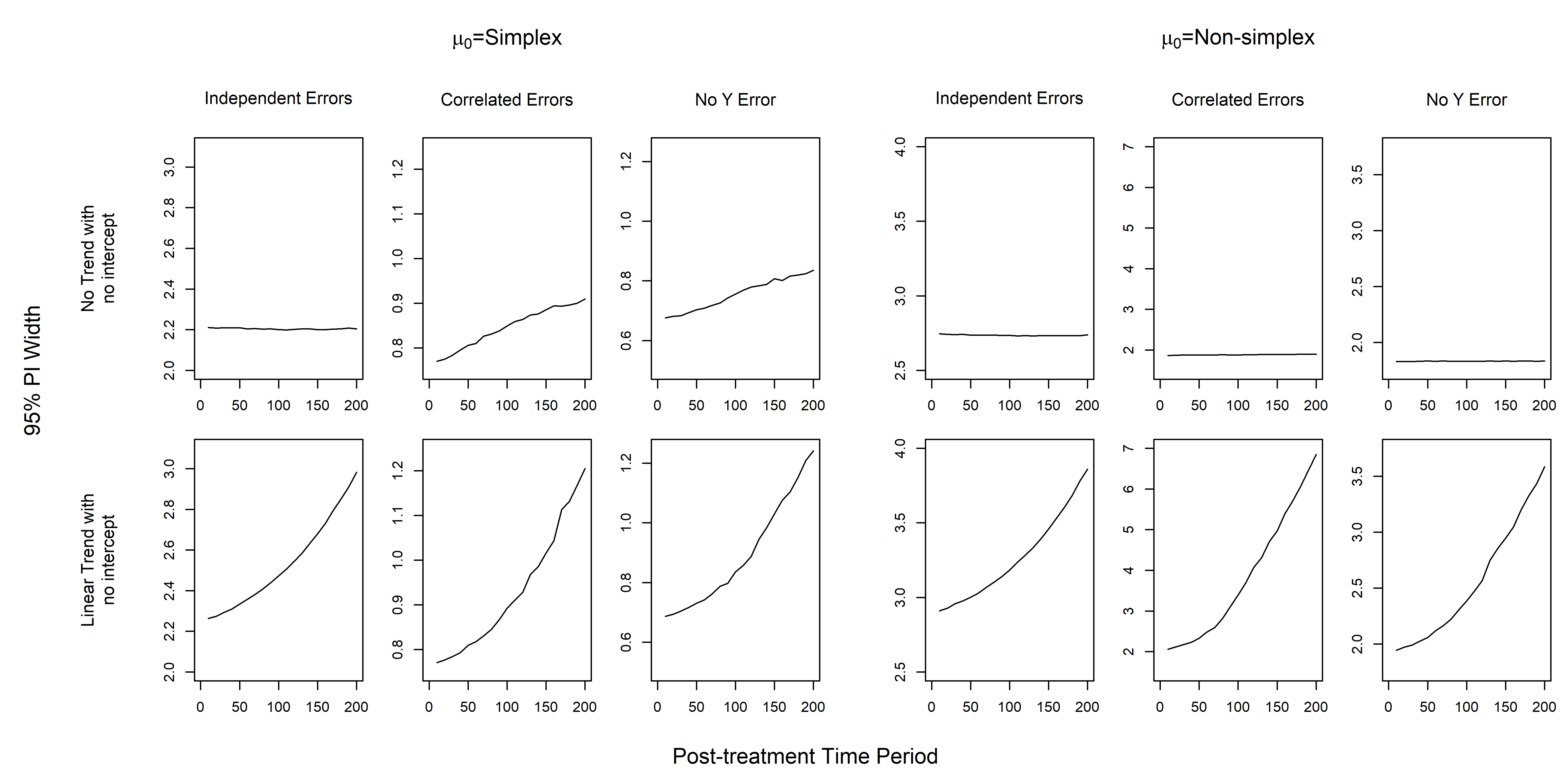
A.9 Simulation Studies under the Scenario Given in Cattaneo et al. 2021
For a fair comparison, we adopt a simulation scenario setup in Cattaneo et al. 2021. In particular, we consider the following data generating process. First, we consider the length of the pre- and post-treatment periods as and . Second, we choose the number of donors as , which are generated from the following AR(1) model:
Here, the autocorrelation coefficient is chosen from , are generated from the standard normal distribution and are independent and identically distributed, and the baseline value is set to zero. For the post-treatment period, we consider the following model for donors:
where parameterizes the degree of the shift in the first donor’s post-treatment outcome. The treatment-free potential outcome of the treated unit is given by
where are independently generated from a standard normal distribution. We consider , i.e., no treatment effect. We remark that is not a valid synthetic control for the SPSC framework because , thereby violating Assumption 3.2. Therefore, the proposed conformal inference approach for the SPSC framework in Section 3.5 may fail in this data generating process.
For our methods, the time-invariant and time-varying pre-treatment estimating equations are given by
where and is the 6-dimensional cubic B-spline bases function.
We repeat the simulation 500 times and calculate the empirical coverage rates of 95% confidence intervals from these repetitions for each simulation scenario. The results are presented in Table 9. First, we find that the SCPI approach achieves the nominal coverage rate across all simulation scenarios in general. However, we find that the conformal inference approach for SPSC without time-varying components (i.e., SPSC-NoDT) fails to achieve the nominal coverage rate, especially when the autocorrelation coefficient is large (i.e., ). We conjecture that the undercoverage observed in these cases may be attributed to the nonstationarity of and . Nevertheless, even in these challenging cases, the conformal inference approach for SPSC with time-varying components (i.e., SPSC-DT) shows significant improvement, attaining the nominal coverage rate across all considered simulation scenarios. This result further confirms that accounting for time-varying components is both useful and necessary for improving the performance of the proposed conformal inference approach in the presence of nonstationarity. Second, regarding the length of the prediction intervals, the SPSC-DT estimator produces the shortest intervals when and . For , the SCPI estimator yields the shortest intervals, although the SPSC-DT estimator remains highly competitive.
| Statistics | Estimators | (second row) and (third row) | ||||||||||||||
| 0 | 0.5 | 1 | ||||||||||||||
| -1 | -0.5 | 0 | 0.5 | 1 | -1 | -0.5 | 0 | 0.5 | 1 | -1 | -0.5 | 0 | 0.5 | 1 | ||
| Coverage | SPSC-NoDT | 0.958 | 0.956 | 0.964 | 0.962 | 0.979 | 0.965 | 0.957 | 0.964 | 0.967 | 0.951 | 0.860 | 0.860 | 0.851 | 0.847 | 0.874 |
| SPSC-DT | 0.952 | 0.954 | 0.964 | 0.962 | 0.974 | 0.961 | 0.951 | 0.952 | 0.959 | 0.943 | 0.953 | 0.941 | 0.937 | 0.942 | 0.947 | |
| SCPI | 0.983 | 0.971 | 0.981 | 0.978 | 0.986 | 0.980 | 0.971 | 0.979 | 0.988 | 0.976 | 0.988 | 0.992 | 0.986 | 0.983 | 0.991 | |
| Length | SPSC-NoDT | 2.303 | 2.317 | 2.313 | 2.321 | 2.325 | 2.445 | 2.469 | 2.462 | 2.464 | 2.449 | 8.169 | 8.596 | 8.531 | 8.970 | 8.346 |
| SPSC-DT | 2.283 | 2.294 | 2.292 | 2.294 | 2.298 | 2.363 | 2.381 | 2.370 | 2.370 | 2.362 | 3.547 | 3.576 | 3.553 | 3.508 | 3.485 | |
| SCPI | 2.546 | 2.543 | 2.582 | 2.573 | 2.569 | 2.580 | 2.569 | 2.554 | 2.588 | 2.575 | 2.985 | 2.999 | 2.966 | 2.962 | 2.973 | |
| Bias | SPSC-NoDT | 0.013 | 0.012 | 0.026 | -0.007 | -0.004 | 0.047 | 0.030 | 0.007 | 0.017 | 0.005 | -0.064 | -0.042 | -0.063 | 0.038 | 0.082 |
| SPSC-DT | 0.015 | 0.010 | 0.025 | -0.002 | -0.005 | 0.041 | 0.028 | 0.009 | 0.011 | 0.001 | 0.014 | -0.007 | 0.004 | -0.006 | -0.002 | |
| SCPI | 0.009 | 0.016 | 0.026 | 0.000 | -0.005 | 0.031 | 0.028 | 0.000 | 0.001 | 0.002 | 0.009 | -0.007 | 0.019 | -0.004 | -0.010 | |
A.10 Additional Results of the Data Analysis
In this Section, we provide additional results of the data analysis in Section 5. First, Figure 9 presents graphical summaries of residuals over the pre-treatment periods. Note that the OLS-NoReg, SCPI, and SPSC-DT estimators produced residuals without a deterministic trend over time, while the other three estimators showed the opposite behavior. Notably, the SPSC-DT estimator appears to satisfy the zero mean condition of Assumption 3.2, whereas the SPSC-NoDT estimator seems to violate this condition due to a non-zero deterministic trend over time. This again highlights the importance of accommodating time-varying components in the SPSC estimation procedure.

Next, we provide the width of the 95% prediction intervals obtained from each method in Figure 10. We remark that the SPSC-DT estimator exhibits relatively stable prediction interval widths compared to the other two methods. It is important to highlight that the stable prediction interval width of the SPSC-DT estimator is specific to this particular dataset. Depending on the underlying data-generating process, the prediction interval width may exhibit greater variability over time. For instance, in some cases illustrated in Figure 8, prediction intervals tens to widen as the post-treatment period progresses. Furthermore, Figure 8 suggests that the width of the SPSC prediction intervals remains stable or shows only a slight increase when there is no systematic drift in the outcomes, but it tends to widen when such drift is present. This systematic drift can be empirically verified by examining the trend of the estimated synthetic control, . As shown in Figure 3 of the main paper, the synthetic control does not exhibit a noticeable upward or downward trend. We hypothesize that this lack of trend explains the stable prediction interval width observed in Figure 10.
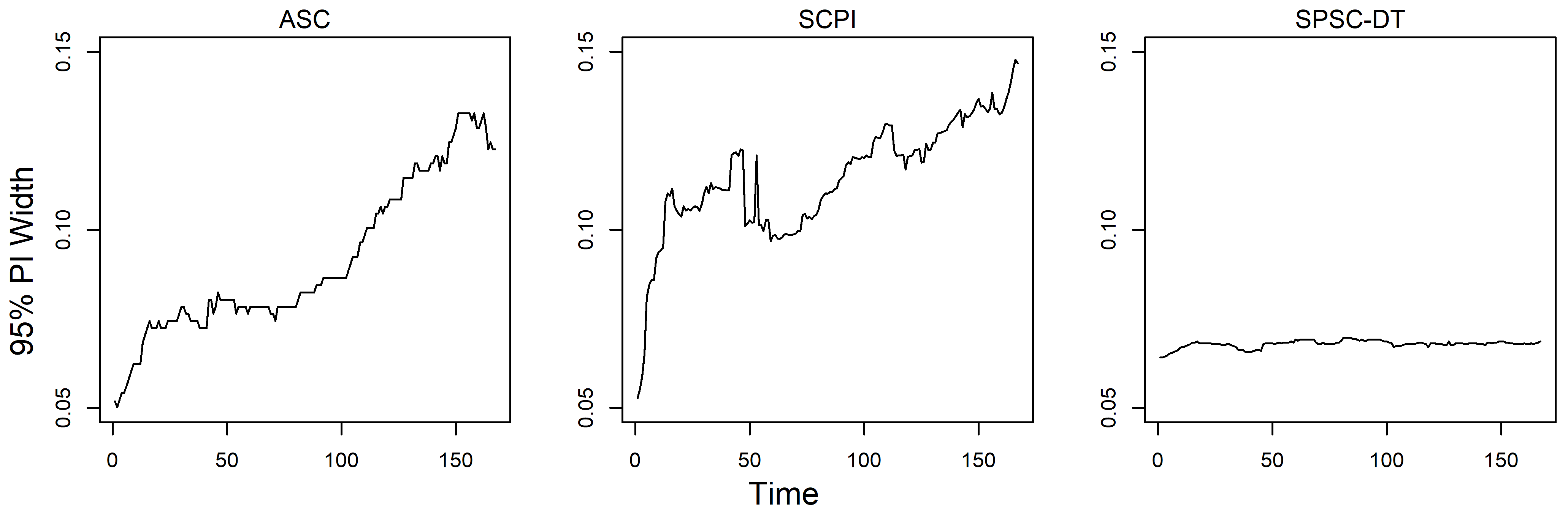
Lastly, we provide the details of the placebo study. Figure 11 visually shows the synthetic controls under the placebo treatment. For the proposed SPSC approach, we find 95% prediction intervals for include the true treatment-free potential outcome for all placebo post-treatment periods. These results suggest that our SPSC approach seems reasonable for analyzing the effect of the 1907 panic on the stock price of the two trust companies. In contrast, the 95% prediction intervals from the SCPI method cover the true treatment-free outcome for 29 placebo post-treatment periods, while the ASC estimator achieves coverage for only 17 periods.

Based on these additional analyses, we can further strengthen the causal conclusions established in the main paper especially those drawn from SPSC, i.e., the 1907 panic led to a decrease in the average log stock price of Knickerbocker and Trust Company of America.
Appendix B Nonparametric Single Proxy Synthetic Control Framework
B.1 Overview
The SPSC framework can be generalized to the case in which the synthetic control is nonlinear and/or nonparametric, thus allowing the outcome to have arbitrary types such as binary, count, and continuous over a bounded interval. The estimation of inference of the synthetic control bridge function and the ATT is analogous to that established in the absence of covariates, so we suppress covariates for notational brevity.
In Section B.2, sufficient conditions for the existence of the synthetic control bridge function is discussed. In Section B.2, we discuss sufficient conditions for the uniqueness of is discussed. Lastly, in Section B.4, we provide details about inference of the ATT without the uniqueness assumption.
B.2 Sufficient Conditions for the Existence of the Synthetic Control Bridge Function
In this Section, we provide sufficient conditions for the existence of the synthetic control bridge function satisfying Assumption A.1. We restate the assumption for readability after suppressing covariates:
Assumption A.1 (Existence of Bridge Function in the Presence of Covariates).
For all , there exists a function that satisfies
In brief, we follow the approach in Miao et al. 2018. The proof relies on Theorem 15.18 of Kress 2014, which is stated below for completeness.
Theorem 15.18. (Kress 2014)
Let be a compact operator with singular system . The integral equation of the first kind is solvable if and only if
To apply the Theorem, we introduce some additional notations. Let and be the spaces of square-integrable functions of and , respectively, which are equipped with the inner products and , respectively. Let be the conditional expectation of given , i.e.,
Then, the synthetic control bridge function solves , i.e.,
Now, we assume the following conditions:
We remark that the expectation can be defined without using under Condition (NPSC-1). First, we show that is a compact operator under Condition (NPSC-2). Let be the conditional expectation of given , i.e.,
Then, and are the adjoint operator of each other as follows:
Additionally, as shown in page 5659 of Carrasco et al. 2007, and are compact operators under Condition (NPSC-2). Moreover, by Theorem 15.16 of Kress 2014, there exists a singular value decomposition of as .
Second, we show that , which suffices to show . Under Condition (NPSC-3), we have
where the first arrow is from the definition of the null space , and the second arrow is from Condition (NPSC-3). Therefore, any must satisfy almost surely, i.e., almost surely.
Third, from the definition of , under Condition (NPSC-4).
Combining the three results, we establish that satisfies the first condition of Theorem 15.18 of Kress 2014. The second condition of the Theorem is exactly the same as Condition (NPSC-5). Therefore, we establish that the Fredholm integral equation of the first kind is solvable under Conditions (NPSC-1)-(NPSC-5).
Note that Conditions (NPSC-1) through (NPSC-5) are sufficient but not necessary. In particular, it is possible to conceive of a scenario where a synthetic control bridge function exists even without the stationarity assumption (NPSC-1). However, this generally requires an additional assumption on the data generating process for (e.g., IFEM) and the form of (e.g., linearity) to ensure stationary behavior in ; see Section A.5 for a specific example. As a result, case-specific models and assumptions are needed to account for non-stationary behavior in the outcomes. Since the purpose of this section is to demonstrate the possibility of relaxing the linearity of the synthetic control bridge function under stationarity, we do not further explore other cases without stationarity here. We intend to pursue this direction in future research.
B.3 Uniqueness of Synthetic Control Bridge Function Under Completeness
We provide a sufficient condition for the uniqueness of the bridge function. Consider the following completeness assumption:
Assumption B.1 (Completeness).
For , suppose almost surely for a square integrable function . Then, almost surely for .
The assumption states that should be -relevant for all time periods in the sense that any variation in is captured by variation in .
Let and be the synthetic control bridge functions satisfying Assumptions 2.1, 2.2, A.1, and A.1, and B.1. We then find , implying and for all , implying that a function satisfying A.1 is unique.
We remark that Assumption B.1 may not be satisfied if the cardinality of the support of is strictly larger than that of . For instance, suppose that the outcomes are binary and two donors are available, i.e., and . Then, the equation in Assumption B.1 reduces to
| (41) |
where . Since (41) is an underdetermined system, there are multiple non-zero functions satisfying (41), indicating that Assumption B.1 cannot be satisfied.
In the following section, we introduce a nonparametric SPSC framework that accommodates non-unique synthetic control bridge functions.
B.4 Single Proxy Synthetic Control Approach without the Uniqueness Assumption
The synthetic control bridge function is defined as a function satisfying (39); we restate the equation below for readability.
| (39) |
We consider the case where there are multiple synthetic control bridge functions satisfying (B.4). Even so, identification of the ATT established in Theorem A.1 is satisfied regardless of the choice of the bridge function. However, estimation and inference of the ATT can be complicated in the presence of multiple synthetic control bridge functions. To resolve this issue, we use approaches proposed by a series of recent works (Li et al. 2023; Zhang et al. 2023). In brief, their approaches involve the following three stages. In the first stage, we estimate a set of synthetic control bridge functions based on a sieve estimator; see Stage 1 below. In the second stage, we define a criterion function, denoted by , and focus on the estimation of the minimizer of , denoted by . Then, an estimator of the ATT can be constructed based on the estimator of ; see Stage 2 below. In the third stage, we consider a de-biasing procedure for the estimator obtained in the previous stage to attain the asymptotic normality; see Stage 3 below. The following sections present details under general nonparametric settings, but the method can be applied to the parametric synthetic controls, including cases where there are multiple synthetic control weights that satisfy Assumption 3.2. We have included only the essential assumptions and notations in this work to ensure clarity. We refer the readers to Li et al. 2023 and Zhang et al. 2023 for additional details.
Stage 1: Estimation of the Solution Set
Let be a collection of user-specified smooth functions, and let be the collection of the solutions of (B.4), i.e.,
Alternatively, we can represent using a criterion function. Let be a criterion function having the following form:
It is straightforward to check that .
We consider a sieve approach as follows. First, we choose a sequence of approximating bases functions of , denoted by . For this sequence, we define an approximating function space for by using the first bases functions, i.e.,
where is a known parameter and are unknown scalar parameters.
A sample analogue of the criterion function , denoted by , can be obtained based on the sieve approach. We choose a sequence of approximating bases functions of , denoted by . Then, we choose the first bases function and construct a -dimensional function of , denoted by . Using the pre-treatment observations, we construct a matrix as follows:
For a given function , a sieve estimator of the conditional expectation for can be obtained by regressing on , i.e.,
Therefore, can be obtained based on a sieve estimator, i.e.,
The proposed estimator of is
where is an appropriately chosen sequence with as . Under regularity conditions, we have
where is the Hausdorff distance between and with respect to a given norm ; see Section 3.2 of Li et al. 2023 and Section 3.2 of Zhang et al. 2023 for details.
Stage 2: A Representer-based Estimator
After obtaining a consistent set estimator of (i.e., ), we select an estimator of from so that it converges to a unique element in . Specifically, we define a function that has a unique minimum on . Let be its sample analogue, and let be the minimum of over , i.e.,
To obtain a unique minimum , and are chosen to satisfy the following assumption:
Assumption B.2.
The following conditions are satisfied:
- 1.
The set is convex;
- 2.
The functional is strictly convex, and have a unique minimum at on ;
- 3.
The sample analogue is continuous and .
Possible choices for and its sample analogue are
Under regularity conditions, we have ; see Theorem 3 of Li et al. 2023 and Proposition 3.2 of Zhang et al. 2023 for details. In turn, we obtain an estimator of the ATT as for where inference based on can be established by the conformal inference in Section 3.5 in the Supplementary Material. Alternatively, we may posit a parametric form for the ATT as . Considering as a fixed function, an estimator of can be obtained as a solution to the following equation:
| (42) | ||||
| (43) |
To characterize the asymptotic property of , we additionally define the following objects. Let be
and be the closure of the linear span of under . Then, we assume the following conditions.
Assumption B.3.
The following conditions are satisfied:
- 1.
For any , there exists a function satisfying for .
- 2.
There exists a projection of on , denoted by , which satisfies
where satisfies regularity conditions; see Assumptions 7-10 of Li et al. 2023 and Assumptions 4-7 of Zhang et al. 2023 for details.
We now characterize the asymptotic representation of under regularity conditions including stationarity and independent errors. Applying a first-order Taylor expansion, we find
Therefore, we find that (42) has the following asymptotic representation for :
| (44) | ||||
| (45) | ||||
Following Theorem 4 of Li et al. 2023 and Supplementary Material of Zhang et al. 2023, we establish that (B.4) is . In addition, for , the numerator of (45) is equal to
| (48) |
Here, and its projection are chosen to satisfy Assumption B.3, and is a generic estimator of the conditional expectation operator of the distribution having a fast convergence rate; see Stage 3 below for details on how these estimators are constructed. Combining all results, we have the following result for :
where
Stage 3: A De-biased Estimator
To obtain the asymptotic normality of , we need to de-bias by subtracting an estimated value of . To do so, we define a new criterion function and its sample analogue for as follows:
We obtain an estimator of , denoted by , as
and the resulting estimator of is
Unfortunately, the above estimator is infeasible because it involves with counterfactual outcomes. Therefore, we use as realizations of the treatment-free potential outcomes and construct a matrix as follows:
We consider additional sieve estimators of and for :
Using these sieve estimators, we obtain a feasible estimator of as
Under regularity conditions, we establish that
see Lemma 1 of Li et al. 2023 and Lemma 3.3 of Zhang et al. 2023 for details. Based on this result, we subtract in both hand sides of (48). We then obtain a de-biased estimator as
which is asymptotically normal in that converges in distribution to as where and are given as follows:
Here, is defined in (43) for . The ATT estimator is obtained from the plug-in formula . Consequently, inference of the ATT can be attained based on the standard delta-method applied to the asymptotic normal distribution of .
Appendix C Proof of Theorems
C.1 Proof of Theorems 3.1, 3.2, A.1
We first prove the most general case with a nonlinear bridge function and under the presence of covariates (i.e., Theorem A.1). For the pre-treatment periods , we establish
The first equality holds from Assumption A.1. The second equality holds from Assumption 2.1.
Furthermore, for any , we establish
The first equality holds from Assumption A.1, and the second equality holds from the law of iterated expectation. Therefore, we have
| (49) |
C.2 Proof of Theorems 3.3 and A.2
We denote the collection of parameters as . When there is no covariate as in Section 3.4, we have ; when there are covariates as in Section A.7, we have . In what follows, we focus on the proof of Theorems 3.3 (i.e., the case with no covariates), since the proof of Theorem A.2 follows a similar approach.
C.2.1 Notation
Let the estimating function be where
| (50) |
The derivative of is
where , , .
We denote , , and the parameters of interest as .
Remark C.1.
We will consider a simple case as an example to motivate the assumptions below. Specifically, suppose that and , i.e., constant treatment effect. Then, the estimating function is
| (51) |
Note that the derivative of (51) is
C.2.2 Assumptions
We adapt the proof of Theorem S6 in Qiu et al. 2024 to our setting. First, we introduce regularity conditions that are applicable to general cases, without imposing strict requirements of strong stationarity and ergodicity.
Regularity Condition 1 (Sufficiently Long Pre- and Post-treatment Periods).
As , and for .
Regularity Condition 1 is reasonable if the pre- and post-treatment periods are of roughly the same size and sufficiently large.
Regularity Condition 2 (Compactness).
The parameter space is compact, and ;
Regularity Condition 2 is standard in parametric estimation.
Regularity Condition 3 (Weighting Matrix).
is a positive definite matrix, and converges to a non-random positive definite matrix as .
Regularity Condition 3 is easily satisfied if is chosen as a fixed matrix such as the identity matrix.
Regularity Condition 4 (Population Moment Restriction & Global Identification).
Their exists unique where
Regularity Condition 4 (i) is satisfied if is of full rank. Regularity Condition 4 (ii) is satisfied because the minimum norm solution is uniquely determined. Regularity Condition 4 (iii) is satisfied if is specified based on an identifiable model.
Regularity Condition 5 (Regularity Conditions for ).
The estimating function satisfies
- (i)
is continuous on for each ;
- (ii)
exists and is finite for any ;
- (iii)
is continuous on .
Regularity Condition 5 is satisfied for estimating equation (51) if the following vectors/matrices are finite and well-defined:
| For : | ||||||||||||||
| For : | (52) | |||||||||||||
Regularity Condition 6 (Regularity for & Local Identification).
The function satisfies:
- (i)
exists and is continuous on for each ;
- (ii)
is uniformly bounded for all
- (iii)
exists and is finite;
- (iv)
The column rank of is .
Regularity Condition 6 (i)-(iii) are satisfied for estimating equation (51) if the following vectors/matrices are uniformly bounded:
| For : | |||||||||||||
| For : | |||||||||||||
Regularity Condition 6 (iv) accounts for both underspecified cases (i.e., ) and standard cases (i.e., . We have
where and . Note that the last equality holds from
Therefore, Regularity Condition 6 (iv) holds if and are of column full rank.
Regularity Condition 7 (Smoothness of ).
Let be the solution to
Then, is unique and uniformly bounded. Furthermore, its derivative with respect to , i.e., , is continuous and uniformly bounded.
Regularity Condition 7 states that the parameter for the ATT is a smooth functional of the synthetic control weights .
Regularity Condition 8 (Uniform Weak Law of Large Numbers for ).
Regularity Condition 9 (Uniform Weak Law of Large Numbers for the Gradient of ).
Regularity Conditions 8 and 9 hold if the underlying process is strictly stationary, strongly mixing, or -mixing processes; see Andrews 1988, Pötscher and Prucha 1997 and Qiu et al. 2024 for details.
Regularity Condition 10 (Asymptotic Normality).
As , we have
Here, is a finite valued positive definite matrix.
Assumption 10 directly assumes the asymptotic normality of the sample mean of the estimating function; see Section S2 of Qiu et al. 2024 for the plausibility of the assumption. We remark that Regularity Conditions 8–10 are satisfied under standard assumptions for GMM; see Chapter 3 of Hall 2004 for details.
C.2.3 Proof
Under Regularity Conditions 1–10, we establish the desired result. We simply denote and . For a generic function , we denote
From the form of the estimating equation in (50), we find the following representations for :
where is the function defined in Regularity Condition 7. The synthetic control weight has the following representation. Let and . Then, we find
| If is of full row rank, | |||||
| If is of full column rank, |
Let be the unique minimizer of
From straightforward algebra, we find
As , we find
Let be an arbitrary positive constant. From (C.2.3) and the definition of , the following conditions hold with probability tending to one:
Note that the last inequality holds because is the minimizer of .
These three inequalities imply that
Here .
Let be an arbitrary open set containing . Let us define the following quantity:
Note that is compact under Regularity Condition 2. Also, for a fixed , Regularity Conditions 4 and 5 imply that is positive. Therefore, by taking , the event occurs with probability tending to one, which further implies that . Since is arbitrary chosen, this establishes as for a fixed .
In addition, for any , we find as where
For , we get
Consider a singular vector decomposition of where . Then, we find
Therefore, where the constant does not depend on because and are uniformly bounded for any from Regularity Condition 6 (ii). Likewise, from the mean value theorem, there exists satisfying
Since is uniformly bounded, we find the following result holds for any :
Therefore, for any , we have for a constant . This implies that the convergence is uniform in . Therefore, this implies the double in-probability limit of is well-defined and converge to :
Therefore, taking , we find as .
Next, we establish the asymptotic normality of . First, the following results hold from the assumptions and :
| (54) | ||||
| (55) |
Specifically, (54) holds from Regularity Condition 6-(i) and the continuous mapping theorem. (55) holds from the first-order Taylor expansion, Regularity Condition 10, and .
The first order condition of along with Regularity Condition 6 implies
The third equality is from . The fourth equality is from (54) and (55). The last equality is from (55).
By multiplying , we get
The second equality holds from Regularity Condition 9:
The last equality holds from Regularity Conditions 3, 8, and 9 and the consistency of .
Therefore, we obtain
This implies
Therefore, taking , we have
As a side note, we have
with a counterexample:
Consequently, we find
This concludes the proof.
References
- Abadie et al. (2010) Abadie, A., Diamond, A., and Hainmueller, J. (2010). Synthetic control methods for comparative case studies: Estimating the effect of California’s tobacco control program. Journal of the American Statistical Association, 105(490):493–505.
- Abadie et al. (2011) Abadie, A., Diamond, A., and Hainmueller, J. (2011). Synth: An r package for synthetic control methods in comparative case studies. Journal of Statistical Software, 42(13):1–17.
- Abadie and Gardeazabal (2003) Abadie, A. and Gardeazabal, J. (2003). The economic costs of conflict: A case study of the basque country. American Economic Review, 93(1):113–132.
- Amjad et al. (2018) Amjad, M., Shah, D., and Shen, D. (2018). Robust synthetic control. Journal of Machine Learning Research, 19(22):1–51.
- Anderson and Hsiao (1981) Anderson, T. W. and Hsiao, C. (1981). Estimation of dynamic models with error components. Journal of the American Statistical Association, 76(375):598–606.
- Andrews (1988) Andrews, D. W. K. (1988). Laws of large numbers for dependent non-identically distributed random variables. Econometric Theory, 4(3):458–467.
- Andrews (1991) Andrews, D. W. K. (1991). Heteroskedasticity and autocorrelation consistent covariance matrix estimation. Econometrica, 59(3):817–858.
- Arellano and Bond (1991) Arellano, M. and Bond, S. (1991). Some Tests of Specification for Panel Data: Monte Carlo Evidence and an Application to Employment Equations. The Review of Economic Studies, 58(2):277–297.
- Bai (2009) Bai, J. (2009). Panel data models with interactive fixed effects. Econometrica, 77(4):1229–1279.
- Ben-Michael (2023) Ben-Michael, E. (2023). augsynth: The Augmented Synthetic Control Method. R package version 0.2.0.
- Ben-Michael et al. (2021) Ben-Michael, E., Feller, A., and Rothstein, J. (2021). The augmented synthetic control method. Journal of the American Statistical Association, 116(536):1789–1803.
- Carrasco et al. (2007) Carrasco, M., Florens, J.-P., and Renault, E. (2007). Linear inverse problems in structural econometrics estimation based on spectral decomposition and regularization. In Heckman, J. J. and Leamer, E. E., editors, Handbook of Econometrics, volume 6, pages 5633–5751. Elsevier.
- Carroll et al. (2006) Carroll, R. J., Ruppert, D., Stefanski, L. A., and Crainiceanu, C. M. (2006). Measurement Error in Nonlinear Models: A Modern Perspective. Chapman and Hall/CRC, second edition.
- Cattaneo et al. (2023) Cattaneo, M., Feng, Y., Palomba, F., and Titiunik, R. (2023). scpi: Prediction Intervals for Synthetic Control Methods with Multiple Treated Units and Staggered Adoption. R package version 2.2.2.
- Cattaneo et al. (2021) Cattaneo, M. D., Feng, Y., and Titiunik, R. (2021). Prediction intervals for synthetic control methods. Journal of the American Statistical Association, 116(536):1865–1880.
- Chen (2007) Chen, X. (2007). Chapter 76: Large sample sieve estimation of semi-nonparametric models. volume 6 of Handbook of Econometrics, pages 5549–5632.
- Chernozhukov et al. (2021) Chernozhukov, V., Wüthrich, K., and Zhu, Y. (2021). An exact and robust conformal inference method for counterfactual and synthetic controls. Journal of the American Statistical Association, 116(536):1849–1864.
- Cui et al. (2023) Cui, Y., Pu, H., Shi, X., Miao, W., and Tchetgen Tchetgen, E. (2023). Semiparametric proximal causal inference. Journal of the American Statistical Association, pages 1–12. In Press.
- Donald et al. (2009) Donald, S. G., Imbens, G. W., and Newey, W. K. (2009). Choosing instrumental variables in conditional moment restriction models. Journal of Econometrics, 152(1):28–36.
- Doudchenko and Imbens (2016) Doudchenko, N. and Imbens, G. W. (2016). Balancing, regression, difference-in-differences and synthetic control methods: A synthesis. Technical Report. National Bureau of Economic Research.
- Ferman (2021) Ferman, B. (2021). On the properties of the synthetic control estimator with many periods and many controls. Journal of the American Statistical Association, 116(536):1764–1772.
- Ferman and Pinto (2019) Ferman, B. and Pinto, C. (2019). Synthetic controls with imperfect pre-treatment fit. arXiv: 1911.08521.
- Ferman and Pinto (2021) Ferman, B. and Pinto, C. (2021). Synthetic controls with imperfect pretreatment fit. Quantitative Economics, 12(4):1197–1221.
- Fohlin and Lu (2021) Fohlin, C. and Lu, Z. (2021). How contagious was the panic of 1907? New evidence from trust company stocks. AEA Papers and Proceedings, 111.
- Freedman et al. (2008) Freedman, L. S., Midthune, D., Carroll, R. J., and Kipnis, V. (2008). A comparison of regression calibration, moment reconstruction and imputation for adjusting for covariate measurement error in regression. Statistics in Medicine, 27(25):5195–5216.
- Hall (2004) Hall, A. R. (2004). Generalized Method of Moments. OUP Oxford.
- Hansen (1982) Hansen, L. P. (1982). Large sample properties of generalized method of moments estimators. Econometrica, 50(4):1029–1054.
- Kress (2014) Kress, R. (2014). Linear Integral Equations. Springer, 3 edition.
- Kunsch (1989) Kunsch, H. R. (1989). The Jackknife and the Bootstrap for General Stationary Observations. The Annals of Statistics, 17(3):1217 – 1241.
- Lahiri (1999) Lahiri, S. N. (1999). Theoretical comparisons of block bootstrap methods. The Annals of Statistics, 27(1):386 – 404.
- Li et al. (2023) Li, W., Miao, W., and Tchetgen Tchetgen, E. (2023). Non-parametric inference about mean functionals of non-ignorable non-response data without identifying the joint distribution. Journal of the Royal Statistical Society Series B: Statistical Methodology, 85(3):913–935.
- Liu and Singh (1992) Liu, R. Y. and Singh, K. (1992). Moving blocks jackknife and bootstrap capture weak dependence. In Lepage, R. and Billard, L., editors, Exploring the Limits of Bootstrap. John Wiley, New York.
- Miao et al. (2018) Miao, W., Geng, Z., and Tchetgen Tchetgen, E. J. (2018). Identifying causal effects with proxy variables of an unmeasured confounder. Biometrika, 105(4):987–993.
- Moen and Tallman (1992) Moen, J. and Tallman, E. W. (1992). The bank panic of 1907: The role of trust companies. The Journal of Economic History, 52(3):611–630.
- Newey and West (1987) Newey, W. K. and West, K. D. (1987). A simple, positive semi-definite, heteroskedasticity and autocorrelation consistent covariance matrix. Econometrica, 55(3):703–708.
- Park (2024) Park, C. (2024). R-package for Single Proxy Synthetic Control. R-package version 0.1.0.
- Park et al. (2024) Park, C., Richardson, D. B., and Tchetgen Tchetgen, E. J. (2024). Single proxy control. Biometrics, 80(2):ujae027.
- Pearl (1995) Pearl, J. (1995). Causal diagrams for empirical research. Biometrika, 82(4):669–688.
- Pötscher and Prucha (1997) Pötscher, B. M. and Prucha, I. (1997). Dynamic Nonlinear Econometric Models: Asymptotic Theory. Springer Science & Business Media.
- Qiu et al. (2024) Qiu, H., Shi, X., Miao, W., Dobriban, E., and Tchetgen Tchetgen, E. (2024). Doubly robust proximal synthetic controls. Biometrics, 80(2):ujae055.
- Robbins et al. (2017) Robbins, M. W., Saunders, J., and Kilmer, B. (2017). A framework for synthetic control methods with high-dimensional, micro-level data: Evaluating a neighborhood-specific crime intervention. Journal of the American Statistical Association, 112(517):109–126.
- Shi et al. (2022) Shi, C., Sridhar, D., Misra, V., and Blei, D. (2022). On the assumptions of synthetic control methods. In Camps-Valls, G., Ruiz, F. J. R., and Valera, I., editors, Proceedings of The 25th International Conference on Artificial Intelligence and Statistics, volume 151 of Proceedings of Machine Learning Research, pages 7163–7175. PMLR.
- Shi et al. (2023) Shi, X., Li, K., Miao, W., Hu, M., and Tchetgen Tchetgen, E. (2023). Theory for identification and inference with synthetic controls: A proximal causal inference framework. Preprint arXiv:2108.13935.
- Tchetgen Tchetgen (2013) Tchetgen Tchetgen, E. (2013). The Control Outcome Calibration Approach for Causal Inference With Unobserved Confounding. American Journal of Epidemiology, 179(5):633–640.
- Tchetgen Tchetgen et al. (2024) Tchetgen Tchetgen, E. J., Ying, A., Cui, Y., Shi, X., and Miao, W. (2024). An introduction to proximal causal inference. Statistical Science, 39(3):375 – 390.
- Xu (2017) Xu, Y. (2017). Generalized synthetic control method: Causal inference with interactive fixed effects models. Political Analysis, 25(1):57–76.
- Zhang et al. (2023) Zhang, J., Li, W., Miao, W., and Tchetgen Tchetgen, E. (2023). Proximal causal inference without uniqueness assumptions. Statistics & Probability Letters, 198:109836.