0 \vgtccategoryResearch \authorfooterHuayuan Ye, Chenhui Li, Yang Li, and Changbo Wang are with School of Computer Science and Technology, East China Normal University. Chenhui Li is the corresponding author. E-mail: chli@cs.ecnu.edu.cn.
![[Uncaptioned image]](2307.16176v3/teasor.png)
Since InvVis can embed a large amount of data into images, users can decode the embedded data and perform rich exploration, such as redesigning (a) or reconstructing (b) visualizations, rebuilding a visualization dashboard based on the decoded source code and chart data (c), or visualizing volume data based on the decoded raw data and rendering parameters (d).
Introduction
InvVis: Large-Scale Data Embedding for Invertible Visualization
Abstract
We present InvVis, a new approach for invertible visualization, which is reconstructing or further modifying a visualization from an image. InvVis allows the embedding of a significant amount of data, such as chart data, chart information, source code, etc., into visualization images. The encoded image is perceptually indistinguishable from the original one. We propose a new method to efficiently express chart data in the form of images, enabling large-capacity data embedding. We also outline a model based on the invertible neural network to achieve high-quality data concealing and revealing. We explore and implement a variety of application scenarios of InvVis. Additionally, we conduct a series of evaluation experiments to assess our method from multiple perspectives, including data embedding quality, data restoration accuracy, data encoding capacity, etc. The result of our experiments demonstrates the great potential of InvVis in invertible visualization.
keywords
Information visualization, information steganography, invertible visualization, invertible neural network.Information visualizations are designed to convey information effectively and efficiently. Nowadays, people usually face massive amounts of data. In such cases, the interactivity and operability of a well-designed visualization allow users to perceive information intuitively and quickly. However, these features are often based on certain applications or visualization tools. Typically, the dissemination of visualization charts is based on bitmap images. For example, some users may just take a screenshot of the visualization chart and share it with other people, this leads to the loss of these excellent properties. As a result, it would be meaningful and useful if the initial chart can be recovered from a chart image. In this paper, we call this procedure as invertible visualization, which is concerned with reconstructing or further modifying the visualization from an image.
Some methods have been proposed to address this issue, some of them try to recover the data and visual elements using pattern recognition and object detection techniques [36, 41]. However, these methods generally cannot achieve enough recognition accuracy and have limited applicability. Some other studies have taken a different approach, which is leveraging information steganography, a technique of implicit information embedding. This kind of approach [54, 18, 19] hides chart information in the image in an inconspicuous way and restores the chart by extracting the embedded data. These methods avoid the unstable procedure of identifying chart elements, but they cannot achieve a large steganography capacity while ensuring steganography quality, making it difficult to deal with charts with large amounts of data.
Visualizations containing large amounts of data are ubiquitous, such as large-scale scatter plots, geographic data visualizations, etc. Actually, it is this kind of visualization charts that require more well-designed interactive methods and visual encoding to facilitate users’ understanding and perception of data. However, previous methods cannot handle the invertible visualization of this kind of charts due to their limitations mentioned above. Recently, the field of information steganography has made significant progress. Many studies have successfully hidden arbitrary data or natural images in images without causing significant visual differences. Especially, image steganography based on invertible neural network (INN) [14, 25] has achieved impressive performance. Nevertheless, these methods focus on natural images instead of chart images and chart data. In this paper, we attempt to address the invertible visualization problem of data-intensive charts.
We present a novel method for invertible visualization, called InvVis. InvVis is an end-to-end pipeline that embeds chart information and chart data into chart images in the concealing process and the embedded data can be restored or further reused after the revealing process. InvVis can handle the invertible visualization of charts with large amounts of data, which is different from previous methods. We propose a data-to-image (DTOI) module which can transfer the chart data into data images that can be hidden into images in a less perceivable way. We also outline a concealing and revealing network based on INN that handles the embedding and restoring of information. The data images output by the DTOI module, together with the chart information that is encoded into QR Code [47] image, are embedded into a chart image through the network. And these images can be recovered by the network and transferred back to chart data and chart information. The restored data can be used in various scenarios like redesigning the chart, reorganizing chart data, etc.
We conduct a series of experiments and the results show that the encoded chart image generated by InvVis have better perceptual similarity compared to other methods, and meanwhile the recovered data has less difference. Also, our method can achieve a much larger steganography capacity than previous methods. In summary, our InvVis has great potential in addressing the problem of invertible visualization, especially in cases involving large amounts of data, where our method can handle the problem that previous methods cannot. Our contributions include three aspects:
- (1)
We define the problem of invertible visualization that involves large amounts of data. We present various application scenarios of this problem and conduct corresponding explorations and implementations.
- (2)
We propose a new method of transferring chart data into data images. The data images can effectively represent various kinds of data.
- (3)
We propose a deep learning-based pipeline to embed information into chart images. Our method can achieve high-quality information concealing and revealing with large embedding capacity.
1 Related Work
1.1 Information Steganography
Information steganography is a technique that conceals information in a carrier with limited perceptual changes. The carrier can be various formats of data such as image, text, audio, video, etc. This technique has considerable applications, e.g., digital watermarking, copyright protection and secret communication. An information steganography method is generally evaluated from three aspects: capacity, security and robustness. Capacity means the embedding payload. Security is concerned with the undetectability and imperceptibility of embedded data. Robustness refers to the ability against distortion. Delina et al. [13] proposed a text steganography method to generate steg-text dynamically according to content length and several user-decided options. Hota et al. [21] outlined a pipeline to embed digital watermarks for scientific visualizations. Yang et al. [51] embedded watermarks in a 3D model by modifying its histogram and achieved a fine robustness/distortion trade-off. Delforouzi et al. [12] hid encrypted data into the coefficients of audio in the integer wavelet domain while preserving high audio quality. [42, 57] applied information steganography to carrier videos.
In summary, although previous studies have explored various kinds of carriers, these methods commonly have limited steganography capacity and are not specially designed for information visualization. In our study, a different approach is proposed to address this problem.
1.2 Image Steganography
Image steganography hides data by performing imperceptible changes on a host image. Traditional methods generally alter the image in spatial domain or transform domain. Spatial-domain embedding techniques like Least-Significant Bit (LSB) replacement [30] and Bit Plane Complexity Segmentation (BPCS) [23] modify pixel values subtly to carry information. However, these algorithms fail to preserve the statistical properties of images and are easily detected by steganalysis methods [17, 52]. To address this problem, highly undetectable steganography (HUGO) [34] utilizes high-dimensional image features based on high-order Markov chains to improve algorithm security. Transform domain, e.g., discrete cosine transform (DCT) domain [4] and discrete wavelet-transform (DWT) domain [42, 57], can also be modfied to embed information. Although transform-domain embedding is generally more robust than spatial-domain embedding, both of them can only hide limited bit-level information.
Recently, a variety of deep learning-based image steganography schemes have been proposed and have achieved impressive performance. [56, 43] adopted the autoencoder to embed binary messages in a cover image. [53, 37] used generative adversarial network (GAN) to optimize the distortion of encoded images. There were also various studies that attempted to hide one or more secret images into a carrier image. Baluja et al. [5] first utilized an end-to-end network to learn feature representations of color images and embed them into cover images. Wengrowski et al. [49] introduced a photographic steganography algorithm based on the encoder-decoder network for light field messaging (LFM). Wu et al. [50] proposed to embed multiplane images (MPIs) in a JPEG image and synthesize novel views by decoding it. More recently, the invertible neural network (INN) [25, 14] has been utilized to hide single [22, 27] or multiple [10, 20] images into carrier images.
Most of the aforementioned image steganography methods are designed to hide information in natural images. However, we focus on embedding data into chart images. Chart images typically comprise many homogeneous regions and have different features from natural images. As a result, a different method is required to handle this problem.

1.3 Invertible Visualization
Invertible visualization allows users to regain or further modify the visualization chart from a raster image. The reconstructed chart preserves its initial information including chart type, chart data, interactive methods, visual mapping, etc. This facilitates scenarios such as redesigning the chart, reorganizing chart data, helping visually impaired users to understand chart [11, 40, 35], and enabling reproducibility for scientific visualizations [7].
Previous studies on invertible visualization mainly took two kinds of approaches. First kind of methods aim to extract the information directly from the chart image. Savva et al. [38] used machine learning techniques to infer chart type and underlying data. Poco et al. [35] proposed a pipeline to automatically recover the visual encoding specification of a chart from a raster image. [36] utilized a convolutional neural network (CNN) to extract color mappings from visualization images. Later, some studies tried to improve the extraction performance by introducing human interactions [29, 16] or focusing on certain types of charts [2, 26, 41, 9]. However, this kind of methods are still likely to suffer from insufficient accuracy or limited application scenarios due to the diversity and structural complexity of visualization charts. Another kind of methods embed the metadata of charts in the generated visualization images and reconstruct the chart by decoding the image. VisCode [54] trains an encoder-decoder network to embed and recover QR Codes which contain chart information. To optimize the encoding quality, VisCode leverages a visual importance network to guide the embedding process. Chartem [18] detects the background of chart images and hides metadata by slightly modifying background pixel values. ChartStamp [19] utilizes a distortion layer that simulates real-world image manipulations to improve the robustness. This kind of methods have addressed the abovementioned problem to some extent at a cost of the perceptual quality of chart images. However, to our best knowledge, few previous study has addressed the issue of invertible visualization when the data volume is large. In this paper, we mainly focus on embedding and restoring large amounts of data in the context of information visualization, and we present a new method to implement invertible visualization.
2 Overview
In the field of information visualization, chart plays a critical role in describing and presenting data. Ideally, a well-designed chart should possess properties like user-friendly interactive methods and reasonable demonstration of chart data. These features can improve the efficiency and accuracy for users to cognize and comprehend data, even when the data volume is large at times. Unfortunately, in most cases, visualization charts are disseminated in the form of raster images, forfeiting the aforementioned features. This greatly limits users’ ability to explore and interact with the chart. To solve this problem, we aim to implement invertible visualization by encoding the metadata of the chart into the generated chart image using image steganography techniques.
In this paper, we propose InvVis, a new approach for invertible visualization. Different from previous studies [54, 18, 19], we focus not just on visualization charts with relatively limited amounts of metadata, but also on those with large data volume. Figure 1 shows the pipline of our InvVis, which contains three main components:
- •
Data-to-Image Module To ensure that the chart data enters the concealing network in the form of images, we propose a data-to-image (DTOI) module to implement the data-to-image transfer. This module takes chart data as input and generates several data images representing the data based on the data type. In addition, this module is invertible, which means the original data can be restored by performing the inverse operation of the DTOI module on these images.
- •
Concealing Network The concealing network embeds the metadata of the chart in the carrier image. At first, data images and QR Code image are padded to the same size as the carrier image. Then, these images, including the carrier image, are concatenated and fed into the concealing network. The network produces an encoded image with the same resolution as the carrier image while introducing subtle perturbations.
- •
Revealing Network The revealing network retrieves the metadata from an encoded image. The network first decodes an encoded image to obtain the restored data images and QR Code image. After performing corresponding operations on these images, the restored chart data and chart information are available to users. Users may use the restored data for various applications (e.g., redesigning the chart).

2.1 Definition
In our InvVis, the input comprises three parts, a carrier image , a sequence of chart data , and a plain text that represents the chart information. The DTOI module transfers the chart data to data images . The chart information is encoded into several QR Codes and stitched together into a QR Code image . These images are fed into the concealing network and result in an encoded image . In the revealing process, the revealing network takes an encoded image as input and outputs the restored data images and QR Code image . After that, the restored chart data and chart information can be obtained by performing the reverse DTOI operation and QR Code decoding operation separately. For our InvVis, we aim to make the encoded image perceptually similar to the original chart image, while ensuring that the decoded data is as accurate as possible. Formally, we aim to optimize the two networks and by minimizing:
| (1) |
where and are weight coefficients.
3 Methods
3.1 Dataset
Our dataset can be divided into three parts, which are visualization images, data images and QR Code images.
Visualization Images Visualization images are commonly composed of homogeneous regions, which results in a significant difference from natural images and therefore leads to different image features. Hence, it is not suitable to use a natural image dataset to train our model. Instead, we used a subset of images from VIS30K [8], which is a dataset containing visualizations from various sources, as our visualization image dataset. Specifically, we selected a total of 1500 images and split them into 1200 images as training set and the rest 300 images as testing set.
Data Images We trained our model using data images as input instead of raw chart data. We built our data image dataset with two kinds of data, discrete data and continuous data. For discrete data, we randomly constructed 300 sets of 2-dimensional scatter data. And for continuous data, we first constructed 300 Perlin noise images [33], which are spatial-continuous. To make our dataset more comprehensive, we also selected 380 sets of data from the Earthdata website [15], which include wind field data, ocean current data and other kinds of data with continuity. All types of data mentioned above were transferred into data images using the DTOI module to be discussed in 3.2. We divided these data images into training and testing sets in a 4:1 ratio.
QR Code Images For the purpose of invertible visualization, the chart information is required to be restored from the encoded image with no error. Thus, it is necessary to use a reliable coding scheme to encode this kind of information. There are many coding schemes with error correction (ECC) ability, like Polynomial Code [31], BCH Code [6], etc. However, embedding such kind of binary data can cause perceptible artifacts in the encoded image and also lead to insufficient data recovery accuracy, which is not suitable for the invertible visualization problem. As a result, we leverage QR Code [47], which is a coding scheme with error correction. Although the encoding capacity of QR Code is less than the abovementioned coding schemes, it is easier to embed and can achieve higer data recovery accuracy.
QR Code has different symbol versions (Version 1 to Version 40), and it provides four ECC levels, higher ECC level means higher error correction rate. For more details, we suggest that the reader refer to the specification of ISO/IEC 18004 [1]. In our implementation, we utilize QR Code Version 40 to encode chart information, whose information capacity and error correction capability for different ECC levels is shown in Table 1. In addition, we choose the ‘H’ ECC level, which means about 30% of the error can be fixed. For the training data, we constructed 500 random strings whose length range from 1 to 1273 and converted them into QR Code images.
| ECC Level | Information Capacity | ECC Capability |
|---|---|---|
| ‘L’ (‘Low’) | 2953 characters | About 7% |
| ‘M’ (‘Medium’) | 2331 characters | About 15% |
| ‘Q’ (‘Quality’) | 1663 characters | About 25% |
| ‘H’ (‘High’) | 1273 characters | About 30% |
3.2 Data-to-Image Module
Previous research has proposed various methods to hide data in images. [54, 49] hid QR Codes into images, while [43, 18, 19, 56] directly embedded binary data into images. However, these methods can only achieve limited data embedding capacity. To solve this problem, we propose a data-to-image (DTOI) module, which is a new data coding scheme. The data images output by the DTOI module can be embedded into the carrier image with a larger capacity while bringing less perceptual distortion than previous methods.
In terms of data visualization, most data can be classified into two types: continuous data and discrete data. Our DTOI module performs different operations on these two kinds of data, this process will be described in detail in the following subsections.


3.2.1 DTOI for Continuous Data
Within the realm of data visualization, there are many kinds of continuous data that exhibit spatial continuity in some dimensions, for example, density maps. Although some methods obtain density maps by performing kernel density estimation (KDE) on scatter data, for some data that contains large amounts of scatter points, this is quite time-consuming. In such cases, directly storing the entire density map as a grayscale image can also be a choice. There are many other types of continuous data, vector field data such as wind field and flow field data have spatial continuity in the components of the vectors in each dimension. Volumetric data is another example, it has spatial continuity on every cross-section.
Formally, a sequence of continuous data can be represented as , where is a 2-dimensional plane of spatial-continuous data and is the number of such planes. For instance, is 1 for a density map and 2 for 2-dimensional wind field data. Due to the varying distribution and range of different chart data, we normalize as follows:
| (2) |
where is the normalized while and are the minimum and maximum values in , respectively. After that, we convert each element in to a single-channel grayscale image and obtain data images. In the case when is large (e.g., volumetric data), these data images will be stitched horizontally and vertically to minimize the number of data images, while ensuring that the size of the stitched image does not exceed that of the carrier image. Note that all and , together with the data image stitching information are encoded into QR codes, just like chart information, since the normalized data needs to be de-normalized during the data restoration process.
3.2.2 DTOI for Discrete Data
Discrete data is also very common in the field of information visualization, e.g., 2-dimensional scatter data. For some other kinds of data with higher dimensions, methods such as t-SNE [44] or UMAP [28] are often used to reduce their dimensionality for easier visualization. Most of this kind of data becomes 2-dimensional after dimensionality reduction, thus, the visualization of 2-dimensional discrete data is very common and important. In this paper, we focus on 2-dimensional discrete data. This kind of data generally lacks continuity, either within or between dimensions. If we treat it the same way as we treat continuous data, the result data images will also lack continuity and features, making it difficult for the network to learn feature representations, which in turn leads to unsatisfactory results in data concealing and revealing. As a result, we utilize a novel method to transform discrete data into relatively continuous and smooth data images to solve this problem.
Given a set of 2-dimensional discrete data where is the number of tuples in , we first sort it in ascending order with the first dimension as key, which is, for and in , the former is considered to be larger then the latter if . Then, we divide into groups and sort each group locally with the second dimension as key. This promises that the first dimension data of are close to each other and the second dimension data are in ascending order in each group. This endows the originally discrete and irregular data with a certain continuity. is then normalized and reshaped to obtain 2 grayscale images. To further enhance the continuity of the data images, we insert additional pixels between every two adjacent pixels and use linear interpolation to assign values to them. Specifically, for every pair of adjacent pixels and , the inserted pixel values are:
| (3) |
where is the value of the th inserted pixel and is set to 3 in this paper. Larger can enhance the continuity of data images but decrease the steganography capacity. We also conduct an experiment on how the value of affects the data embedding quality, this will be discussed in 5.1. This algorithm is explained in detail in Algorithm 1. In addition, if the data volume is quite large, the data can be divided into parts and apply this algorithm respectively to generate several data images. These images can then be stitched together to reduce the total channel number of the final data images. Figure 4 shows the 2 data images generated with our algorithm, as we can see, the data images are smooth and continuous. In the data restoring procedure, with the revealed data images output by the revealing network, the restored data can be obtained by selecting and denormalizing those non-inserted pixel values.

As shown in Figure 5, we first embed data images obtained using the above algorithm into a chart image and result in Figure 5(a). For comparison, we also embed data images obtained without sorting and pixel insertion operation into the same chart image and result in Figure 5(b). As we can see, the data images generated with our algorithm can be embedded into images with less distortion.


3.3 Concealing and Revealing Network
Figure 2 shows our concealing and revealing network, which is a symmetric architecture. Both of these two networks are composed of a feature fusion block (FFB) and an invertible steganography network (ISN). In the concealing process, the input carrier image and secret images which consist of QR Code image and data images , are fed into the FFB. To minimize the impact of QR Code image on the distortion of encoded images, we multiply the QR code image by a coefficient before feeding it into the network, and the recovered QR code image is divided by during the decoding procedure. The output of FFB, i.e. and , undergo discrete wavelet transform (DWT) and reshaping separately, they are then concatenated as the input of ISN. The ISN processes its input and results in an encoded image after performing the inverse wavelet transform (IWT) and quantization operation. Since the input and output sizes of ISN are the same, it also outputs a matrix . In the decoding process, an encoded image , together with a constant matrix whose size is the same as that of , goes through the ISN and FFB in sequence to produce the restored data images and QR Code image . Note that in our implementation, the maximum number of the channel that hides information is 4 (3 channels for data images and 1 channel for QR Code image), but it is quite easy to change by slightly modifying the network.
3.3.1 Feature Fusion Block
Previous studies [20, 22, 10, 27] have proposed some methods to hide natural images in each other. The secret images and carrier images in these methods generally have similar natural image features. However, in our InvVis, the secret images to be embedded are data images and QR Code image, they have different data distributions and features from the carrier image. Hence, a different method is needed to reduce the perceptual deviation of the encoded image. To address this issue, we propose the feature fusion block (FFB), attempting to optimize the perceptual quality by blending the features of the carrier image and secret images before the steganography process.
The architecture of our FFB is shown in Figure 6, which is composed of several dense blocks [45] and common convolutional layers. The input of FFB comprises a total of 7 channels, and its output has the same size as the input. In the concealing process, the FFB projects the input into a high-dimensional space and then maps it back to a low-dimensional space, achieving the effect of feature blending. The output of FFB is easier to result in an encoded image with less visual distortion in the following steganography network. The ablation experiment on FFB will be discussed in 5.1. In the decoding process, we also use an FFB to process the output of ISN and obtain the final restored images.
3.3.2 Wavelet Domain Steganography
Spacial-domain steganography can lead to texture-copying artifacts [48], which affects the perceptual quality and is easy to be detected. To improve the concealing performance, we adopt an approach similar to HiNet [22] and DeepMIH [20], which is introducing discrete wavelet transform (DWT). Transferring the image to the wavelet domain before the ISN can guide the network to learn a better embedding strategy that hides more secret information in the high-frequency part of the image rather than the low-frequency part.
Specifically, we perform DWT on , which is part of the output of FFB corresponding to the initial carrier image . Assume that the size of is where , , indicate the channel number, height and width of the image, DWT transfers its size to . In contrast, we do not perform this operation on whose size is , instead, we simply reshape it to for the purpose of size matching. After the hiding process performed by ISN, we use inverse wavelet transform (IWT) to transform the image back to spatial domain and obtain the encoded image. Similarly, In the revealing procedure, a series of symmetric operations are performed to restore the secret images. We conduct the ablation experiment and the result shows that this method can lead to better steganography quality, this will be discussed in 5.1.
3.3.3 Invertible Steganography Network
Our invertible steganography network (ISN) is based on the invertible neural network (INN), which was first proposed by Dinh et al. [14], it allows the secret information to be hidden and revealed in the same network. To enhance the representation ability of the network, we also leverage the invertible 1 1 convolution block proposed by Kingma et al. [25]. Formally, given and , which are the input of ISN corresponding to the carrier image and secret images, the encoded image can be obtained with where is the hiding process and indicates the network parameters. For the revealing procedure, an inverse process which shares the same parameters as can output the restored images and with .
As shown in Figure 2, our ISN is composed of several affine coupling blocks (ACBs). Each ACB shares the same parameters in the hiding and revealing process but has an opposite data flow direction. Assume that the input of the th ACB is and indicating the carrier image and secret image channels, the invertible convolution block outputs and with their size not changed:
| (4) |
where indicates the forward procedure of invertible convolution. After that, the output of this ACB can be formulated as:
| (5) |
in which is the exponential function, is the Hadamard product and , , are functions learned by convolution blocks. There can be a variety of choices for the type of these convolution blocks, in this paper, we use dense block [45] due to its powerful representation ability. In the revealing procedure, the output of the th ACB can be obtained by reformulating Equation 4 and Equation 5 like:
| (6) |
and
| (7) |
where is the inverse operation of .
Since the input and output of ISN are the same, we only extract the first 12 channels from the output and perform IWT to obtain the final encoded image. Similarly, in the revealing process, we perform DWT on the encoded image and pad it with a constant matrix to match its size to that of the input of ISN.
Figure 7demonstrates a comparison of the image quality before and after data embedding. Figure 7(c) shows the difference between the original chart image and the encoded image. We enhance the residual by 2 times to more clearly show the difference. As we can see, our method can embed data into images while preserving the perceptual quality of the image.


3.3.4 Loss Function
The optimization of our network can be divided into two parts, which are the perceptual quality of the encoded image and the restoration accuracy of secret images. We utilize hybrid loss functions to train our model in order to achieve better performance.
Given a carrier image and an encoded image , we define our encoding loss as:
| (8) |
where is a weight coefficient and measures the mean squared error (MSE) of pixel values between and . Inspired by Jing et al. [22], we introduce to measure and optimize the low-frequency sub-bands difference after wavelet decomposition. Assume that output the low-frequency sub-bands of image, can be defined as:
| (9) |
For restoration accuracy, we use both L1 and MSE loss function to guide the training process, the restoration loss of secret images can be defined as:
| (10) |
where and denotes the th secret image and its corresponding restored image respectively. In summary, the total loss function of our network can be formulated as:
| (11) |
where is another weight coefficient just like .
4 Applications
Our InvVis is competent in various scenarios, such as embedding URL or copyright information in a visualization, which has been discussed in [54]. Compared to previous methods, our approach has the advantage of being applicable to scenarios that involve large amounts of data. For instance, it can facilitate invertible visualization of data-intensive charts, large-scale source code embedding and scientific data embedding.

4.1 Invertible Visualization of Data-Intensive Chart
Data-intensive charts are common in the field of information visualization. Due to the large data volume they contain, such charts generally require some interactive functionalities to assist users in comprehending the data. However, there is a lack of a convenient way to disseminate this kind of visualization while preserving their interactivity. InvVis enables the reconstruction of interactive charts from a single image, greatly simplifying their dissemination. Figure 8 shows the application interface of our InvVis. In the data embedding process, the user can upload a chart image and its metadata, including the chart data and chart information, the application can embed the uploaded data into the chart image and output an encoded image. In the data restoring procedure, the application can decode an encoded image and reconstruct the interactive chart.
InvVis can also facilitate the reusing of chart data. Since it allows to hide all the original data into the chart image, users can have full access to all the metadata of the chart after decoding and restoring the data. The recovered data contains not only the chart information but also the underlying data, which means that users may further reuse the data. As shown in Figure 9, apart from reconstructing the chart, users may redesign the chart from various perspectives with the decoded metadata, such as changing the visual mapping of the chart. Also, the chart data can be reorganized and mapped to new visualizations. For example, users can compute the statistics of the chart data and map it to a doughnut chart.


4.2 Large-Scale Source Code Embedding
Source code is an important part of visualizations. Some visualization charts may contain a large amount of source code due to their sophisticated interactive methods or large data volume. VisCode [54] proposed to hide the source code in a chart image, but due to the limited steganography capacity of this method, it cannot handle the cases in which the amount of source code or data is quite large. As will be discussed in 5.2, InvVis has a much larger steganography capacity than VisCode, even when only hiding QR Codes, which can be indicated by Table 5. Therefore, our method can better handle this problem.
To better illustrate the practicality of large-scale source code embedding, we present an application scenario, which is the visualization dashboard. Visualization dashboard is a collection of various visualization charts that are displayed together on a single screen or interface. It can be used in business intelligence or data analysis to provide a quick overview of key metrics and statistical data. Since a visualization dashboard generally contains several visualization charts, the amount of its metadata may be much larger than that of a single chart. Additionally, if the chart data is also written directly in the source code, it will make the source code very long. For methods like VisCode that encode all the source code into QR Codes, the number of QR Codes can be too large to be hidden in the carrier image. Meanwhile, if a relatively small image is used to display a visualization dashboard, the charts and data contained in it may be too small to be clearly seen. Therefore, if the source code, together with the chart data of a visualization dashboard can be effectively hidden in an image, it can greatly facilitate the dissemination of this kind of visualization.
InvVis can handle this problem in a novel way. Since InvVis can hide both data images and QR Code image simultaneously, we can separate the data with large volume from the source code and transfer them to data images. This effectively reduces the length of the source code, and meanwhile increases the efficiency of data embedding. Our method allows both the data and source code to be carried by a relatively smaller carrier image. Figure 10 demonstrates an example, the source data of the heat map is separated from the source code and transferred into data images. The data images and the QR Code image that contains the source code are embedded into a relatively small image. By decoding this image, users can obtain a complete and interactive visualization dashboard.

4.3 Scientific Data Embedding
Scientific data typically has large data volume, such as terrain data, ocean current data, volumetric data, etc. These kinds of data generally require visualization methods to present the data and design some interactive ways to facilitate researchers or common users in understanding the data intuitively. Since our InvVis can effectively embed data into carrier images through data images, it has great potential for the embedding of scientific data. This allows users to spread scientific visualizations through a single image.
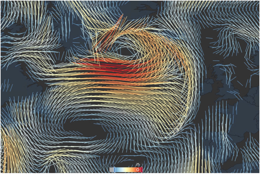
Figure 11(a)(b)(c) shows an example of scientific data embedding. We embed a set of wind field data which contains a total of 35180 2-dimensional vectors into an image. Although the data volume is quite large, the size of the carrier image is as small as 520 360. Figure 11(b)(c) shows the reconstructed visualization, which is interactive, allowing users to query data within a certain range or zoom in to view the distribution of data in a specific area. Figure 11(d)(e)(f) demonstrates another example, we embed the volumetric data of an engine into a carrier image. The amount of this volumetric data is very large, reaching 256 256 128, while in contrast, the carrier image is only 2304 1280. Our method can effectively hide such a large amount of data into the carrier image and results Figure 11(d), whose distortion is almost unobservable. And the restored data is also very accurate, as shown in Figure 11(e)(f), the reconstructed visualization is indistinguishable from the original one and allows users to view the volume data visualization from different directions.



5 Evaluation
We evaluate our method from two aspects, steganography quality and steganography capacity, which are two of the most important criteria for information steganography. We conduct our experiments on a PC with an Intel Core i7 CPU, an NVIDIA GeForce 3090 GPU, and 64 GB of memory. Our model is implemented with PyTorch [32]. We use 32 ACBs in our ISN and train our model using the Adam optimizer [24]. The weight coefficients of the loss function (Equation 11) are set as and to balance the data embedding quality and data restoration accuracy. In addition, as mentioned in subsection 3.1, our experiments are conducted on our test dataset.
5.1 Steganography Quality
Steganography quality refers to both the perceptual quality of the encoded image and the accuracy of restored information. These two criteria are inversely related to each other, which means higher embedding quality generally leads to lower data restoration capacity and vice versa. A good steganography method should achieve a satisfactory trade-off between them.
We evaluate the quality of encoded image using three metrics, which are the peak signal-to-noise ratio (PSNR) [3], the structural similarity index (SSIM) [46] and the learned perceptual image patch similarity (LPIPS) [55]. The PSNR is often used to evaluate the distortion of images, and the SSIM measures the structural similarity between two images. The LPIPS is based on the high-level features of images, which represent the perceptual similarity between two images. In our experiments, we use VGG [39] as the feature extraction network for the calculation of LPIPS. Higher PSNR, SSIM and lower LPIPS is better.
For the data restoration accuracy, we use root mean squared error (RMSE) to measure the difference between the initial data images and the restored data images. In addition, we use the text recovery accuracy (TRA) [54], which refers to the proportion of the restored characters among all input characters, to measure the performance of QR Code image recovery. Lower RMSE and higher TRA is better.


We first conduct a series of ablation experiments to investigate the impact of FFB and wavelet domain steganography on the final perceptual quality of the encoded image. We hide 3 channels of data images and one channel of QR Code image into each carrier image. Each QR Code image is encoded with characters and . As shown in Table 2, our full model achieves the best balance between information embedding quality and data restoration accuracy.
| Method | PSNR | SSIM | LPIPS | RMSE | TRA |
|---|---|---|---|---|---|
| Ours w/o wavlet | |||||
| Ours w/o FFB | |||||
| Ours | 44.6889 | 0.9830 | 0.0120 | 0.0062 | 0.9892 |
In addition, we experiment on how the linear interpolation discussed in 3.2.2 affects the steganography quality. We regenerate the scatter data images in our dataset with different values of and retrain the model, and then we evaluate it on the corresponding test set (contains scatter data images only). The result is shown in Table 3. As we can see, larger can lead to better steganography quality at the cost of lower steganography capacity.
| K value | PSNR | SSIM | LPIPS | RMSE | TRA |
|---|---|---|---|---|---|
| 0 | |||||
| 1 | |||||
| 3 | |||||
| 7 |
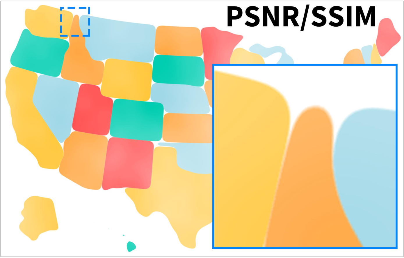
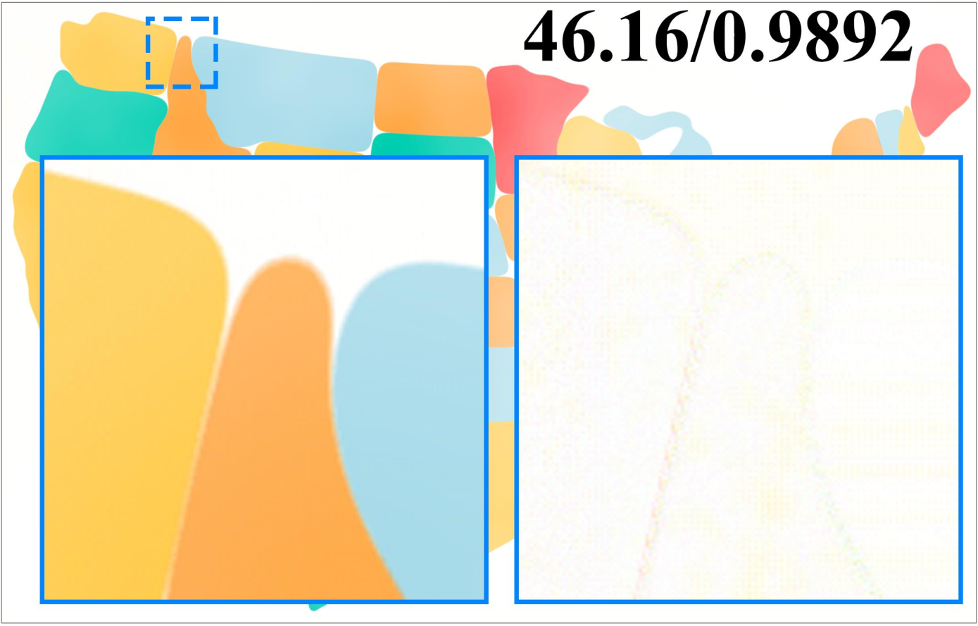
We also compare our model with other image steganography methods, i.e. HiNet [22] and IICNet [10]. We hide 2 channels of data images and one channel of QR Code image into each carrier image. Figure 12 shows a comparison between the encoded image generated by our method with Hinet and IICNet. The magnified area and its corresponding residual (enhanced by 4 times), along with the PSNR and SSIM of the encoded images are shown. As we can see, InvVis can generate encoded images that are more perceptually similar to the carrier image and has less distortion. The results of the comparative experiments are shown in Table 4, in which we can see that our model achieves the best performance on both steganography quality and data restoration accuracy.
5.2 Steganography Capacity
The capacity of steganography concerns how much chart information can be concealed in the image, which is crucial for the invertible visualization of charts with large amounts of data. There is also a trade-off between steganography capacity and quality, larger steganography capacity can lead to lower quality of the encoded image.
To measure the steganography capacity of different methods, we use bits per pixel (BPP), which indicates the average number of bits hidden in the encoded image per pixel, as the metric. Formally, given a carrier image whose size is , its BPP is calculated as:
| (12) |
where is the total number of bits hidden in .
We compare our method with VisCode [54]. VisCode uses a region proposal algorithm based on saliency detection to choose the places to hide QR Code images. Although this method can achieve better image encoding quality than using predetermined regions for data embedding, it cannot guarantee that the image is maximally utilized to hide data. Also, if the encoded data volume is large, VisCode cannot achieve a satisfactory embedding quality. In contrast, our method concatenates the QR codes horizontally and vertically into QR Code images to maximize spatial utilization, and our method can achieve good steganography quality even if the data volume is large.
We first compare the steganography capacity of our method with VisCode when only hiding QR Codes. Since our methods can not only hide QR Code image but also hide data images, we also compare the maximum steganography capacity of our method with VisCode. The result is shown in Table 5, as we can see, our method achieves a larger steganography capacity than VisCode even when only hiding QR Code image, and our maximum steganography capacity far exceeds that of VisCode. Moreover, the quality of the encoded image is also much better than that of VisCode in both experiments. Besides, the average computational time of encoding and decoding, together with the model size of VisCode and InvVis are also shown in Table 5. As we can see, InvVis has a smaller model size and faster computational speed.
| Method | Time | Size | PSNR | SSIM | LPIPS | BPP |
|---|---|---|---|---|---|---|
| VisCode [54] | 4.9/2.6 | mb | 29.8098 | 0.9499 | 0.0682 | 0.0049 |
| Ours (QR only) | 3.0/2.2 | 158mb | 45.1067 | 0.9851 | 0.0073 | 0.0218 |
| Ours (maximum) | 44.5082 | 0.9822 | 0.0131 | 5.5218 |
We also compare the steganography quality of our method under different BPP values. We divide the BPP into three levels, which are low, medium and maximum. The BPP value of different levels and the corresponding steganography quality are shown in Table 6, as we can see, InvVis can maintain high steganography quality under different levels of BPP.
| BPP Level | BPP | PSNR | SSIM | LPIPS |
|---|---|---|---|---|
| Low | 0.5458 | 46.0429 | 0.9893 | 0.0051 |
| Medium | 2.7604 | 45.5163 | 0.9868 | 0.0104 |
| Maximum | 5.5218 | 44.5082 | 0.9822 | 0.0131 |
6 Conclusion
We propose InvVis, a new approach for embedding information into visualization images, which is suitable for cases with large amounts of data. Our InvVis can support various application scenarios like invertible visualization of data-intensive charts, large-scale source code embedding, scientific data embedding, etc. We propose a new method to transfer chart data into images that can be more easily embedded in chart image with high quality. We also outline a deep learning-based pipeline to embed information into chart images. Our evaluation experiments show that InvVis can achieve high-quality information concealing and revealing with large steganography capacity.
The current version of InvVis has certain limitations in addressing invertible visualization problems with zero tolerance for errors. In addition, the steganography capacity of InvVis is related to the size of the carrier image, it may not achieve a satisfactory embedding capacity if the image size is too small. Also, InvVis is mainly designed to facilitate chart image transmission on the internet, so it lacks stability when facing real-world image interference such as printing and shooting.
In the future, we plan to propose a more widely applicable method that can handle more types of data and achieve better steganography performance and recovery accuracy while ensuring steganography capacity. Additionally, as shown in the work of Tancik et al. [43] and Fu et al. [19], the method can be more robust if it is stable against some steganography attacks, this is also a potential research direction.
Acknowledgements.
The authors wish to acknowledge the support from NSFC under Grants (No. 62102152, 62072183 and 61802128), Shanghai Municipal Science and Technology Major Project (Grant No. 22511104600), and CAAI-Huawei MindSpore Open Fund.References
- [1] Information technology — automatic identification and data capture techniques — qr code bar code symbology specification. ISO/IEC 18004:2015, 2015.
- [2] R. Al-Zaidy and C. Giles. A machine learning approach for semantic structuring of scientific charts in scholarly documents. In Proc. AAAI Conf. Artif. Intell., pp. 4644–4649, 2017.
- [3] A. Almohammad and G. Ghinea. Stego image quality and the reliability of psnr. In 2nd Intl. Conf. Image Process. Theory Tools Appl., pp. 215–220. IEEE, 2010.
- [4] A. Almohammad, R. M. Hierons, and G. Ghinea. High capacity steganographic method based upon jpeg. In Intl. Conf. Availability Reliability Security, pp. 544–549. IEEE, 2008.
- [5] S. Baluja. Hiding images in plain sight: Deep steganography. Adv. Neural Inf. Process. Syst. (NIPS), 30, 2017.
- [6] R. C. Bose and D. K. Ray-Chaudhuri. On a class of error correcting binary group codes. Inf. Control., 3:68–79, 1960.
- [7] S. P. Callahan, J. Freire, E. Santos, C. E. Scheidegger, C. T. Silva, and H. T. Vo. Vistrails: Visualization meets data management. In Proceedings of the 2006 ACM SIGMOD International Conference on Management of Data, SIGMOD ’06, p. 745–747. Association for Computing Machinery, New York, NY, USA, 2006. doi: 10.1145/1142473.1142574
- [8] J. Chen, M. Ling, R. Li, P. Isenberg, T. Isenberg, M. Sedlmair, T. Möller, R. S. Laramee, H.-W. Shen, K. Wünsche, and Q. Wang. VIS30K: A collection of figures and tables from IEEE visualization conference publications. IEEE Trans. Visual. Comput. Graph., 27(9):3826–3833, Sept. 2021. doi: 10.1109/TVCG.2021.3054916
- [9] Z. Chen, Y. Wang, Q. Wang, Y. Wang, and H. Qu. Towards automated infographic design: Deep learning-based auto-extraction of extensible timeline. IEEE Trans. Visual. Comput. Graph., 26(1):917–926, 2019.
- [10] K. L. Cheng, Y. Xie, and Q. Chen. Iicnet: A generic framework for reversible image conversion. In Proc. IEEE/CVF Intl. Conf. Comput. Vis., pp. 1991–2000, 2021.
- [11] J. Choi, S. Jung, D. G. Park, J. Choo, and N. Elmqvist. Visualizing for the non-visual: Enabling the visually impaired to use visualization. In Comput. Graph. Forum, pp. 249–260. Wiley Online Library, 2019.
- [12] A. Delforouzi and M. Pooyan. Adaptive digital audio steganography based on integer wavelet transform. Circuits Syst. Signal Process., 27(2):247–259, 2008.
- [13] B. Delina. Information hiding: A new approach in text steganography. In Intl. Conf. Appl. Comput. Appl. Comput. Sci. (WSEAS), pp. 689–695, 2008.
- [14] L. Dinh, D. Krueger, and Y. Bengio. Nice: Non-linear independent components estimation. CoRR, abs/1410.8516, 2014.
- [15] N. Earth Science Data Systems. Earthdata.
- [16] A. Flower, J. W. McKenna, and G. Upreti. Validity and reliability of graphclick and datathief iii for data extraction. Behav. Modif., 40(3):396–413, 2016.
- [17] J. Fridrich, M. Goljan, and R. Du. Detecting lsb steganography in color, and gray-scale images. IEEE Multimed., 8(4):22–28, 2001.
- [18] J. Fu, B. Zhu, W. Cui, S. Ge, Y. Wang, H. Zhang, H. Huang, Y. Tang, D. Zhang, and X. Ma. Chartem: reviving chart images with data embedding. IEEE Trans. Visual. Comput. Graph., 27(2):337–346, 2020.
- [19] J. Fu, B. B. Zhu, H. Zhang, Y. Zou, S. Ge, W. Cui, Y. Wang, D. Zhang, X. Ma, and H. Jin. Chartstamp: Robust chart embedding for real-world applications. In Proc. 30th ACM Intl. Conf. Multimedia, pp. 2786–2795, 2022.
- [20] Z. Guan, J. Jing, X. Deng, M. Xu, L. Jiang, Z. Zhang, and Y. Li. Deepmih: Deep invertible network for multiple image hiding. IEEE Trans. Pattern Anal. Mach. Intell., 45(1):372–390, 2022.
- [21] A. Hota and J. Huang. Embedding meta information into visualizations. IEEE Trans. Visual. Comput. Graph., 26(11):3189–3203, 2019.
- [22] J. Jing, X. Deng, M. Xu, J. Wang, and Z. Guan. Hinet: Deep image hiding by invertible network. In Proc. IEEE/CVF Intl. Conf. Comput. Vis., pp. 4733–4742, 2021.
- [23] E. Kawaguchi and R. O. Eason. Principles and applications of bpcs steganography. In Multimedia Syst. Appl., vol. 3528, pp. 464–473. SPIE, 1999.
- [24] D. P. Kingma and J. Ba. Adam: A method for stochastic optimization. CoRR, abs/1412.6980, 2014.
- [25] D. P. Kingma and P. Dhariwal. Glow: Generative flow with invertible 1x1 convolutions. Adv. Neural Inf. Process. Syst. (NIPS), 31, 2018.
- [26] X. Liu, D. Klabjan, and P. N. Bless. Data extraction from charts via single deep neural network. arXiv, abs/1906.11906, 2019.
- [27] S.-P. Lu, R. Wang, T. Zhong, and P. L. Rosin. Large-capacity image steganography based on invertible neural networks. In Proc. IEEE/CVF Conf. Comput. Vis. Pattern Recognit., pp. 10816–10825, 2021.
- [28] L. McInnes, J. Healy, and J. Melville. UMAP: Uniform Manifold Approximation and Projection for Dimension Reduction. arXiv e-prints, Feb. 2018.
- [29] G. G. Méndez, M. A. Nacenta, and S. Vandenheste. ivolver: Interactive visual language for visualization extraction and reconstruction. In Proc. 2016 CHI Conf. Hum. Factors Comput. Syst., pp. 4073–4085, 2016.
- [30] J. Mielikainen. Lsb matching revisited. IEEE Signal Process. Lett., 13(5):285–287, 2006.
- [31] F. Moore, W. J. Brady, and F. J. Telecky. Polynomial codes over certain finite fields. 2017.
- [32] A. Paszke, S. Gross, F. Massa, A. Lerer, J. Bradbury, G. Chanan, T. Killeen, Z. Lin, N. Gimelshein, L. Antiga, et al. Pytorch: An imperative style, high-performance deep learning library. Adv. Neural Inf. Process. Syst. (NIPS), 32, 2019.
- [33] K. Perlin. An image synthesizer. ACM SIGGRAPH Comput. Graph., 19(3):287–296, 1985.
- [34] T. Pevnỳ, T. Filler, and P. Bas. Using high-dimensional image models to perform highly undetectable steganography. In Information Hiding, IH, pp. 161–177. Springer, 2010.
- [35] J. Poco and J. Heer. Reverse-engineering visualizations: Recovering visual encodings from chart images. In Comput. Graph. Forum, pp. 353–363. Wiley Online Library, 2017.
- [36] J. Poco, A. Mayhua, and J. Heer. Extracting and retargeting color mappings from bitmap images of visualizations. IEEE Trans. Visual. Comput. Graph., 24(1):637–646, 2017.
- [37] J. Qin, J. Wang, Y. Tan, H. Huang, X. Xiang, and Z. He. Coverless image steganography based on generative adversarial network. Math., 8(9):1394, 2020.
- [38] M. Savva, N. Kong, A. Chhajta, L. Fei-Fei, M. Agrawala, and J. Heer. Revision: Automated classification, analysis and redesign of chart images. In Proc. 24th Annu. ACM Symp. User Interface Softw. Technol., pp. 393–402, 2011.
- [39] K. Simonyan and A. Zisserman. Very deep convolutional networks for large-scale image recognition. In Y. Bengio and Y. LeCun, eds., 3rd Intl. Conf. Learn. Representations (ICLR), 2015.
- [40] M. Singh and P. Goyal. Chartsight: An automated scheme for assisting visually impaired in understanding scientific charts. In VISIGRAPP (5: VISAPP), pp. 309–318, 2021.
- [41] S. Song, C. Li, D. Li, J. Chen, and C. Wang. Graphdecoder: Recovering diverse network graphs from visualization images via attention-aware learning. IEEE Trans. Visual. Comput. Graph., 2022.
- [42] M. D. Swanson, B. Zhu, B. Chau, and A. H. Tewfik. Multiresolution video watermarking using perceptual models and scene segmentation. In Proc. Intl. Conf. Image Process., vol. 2, pp. 558–561. IEEE, 1997.
- [43] M. Tancik, B. Mildenhall, and R. Ng. Stegastamp: Invisible hyperlinks in physical photographs. In Proc. IEEE/CVF Conf. Comput. Vis. Pattern Recognit., pp. 2117–2126, 2020.
- [44] L. Van der Maaten and G. Hinton. Visualizing data using t-sne. J. Mach. Learn. Res., 9(11), 2008.
- [45] X. Wang, K. Yu, S. Wu, J. Gu, Y. Liu, C. Dong, Y. Qiao, and C. Change Loy. Esrgan: Enhanced super-resolution generative adversarial networks. In Proc. Eur. Conf. Comput. Vis. (ECCV) Workshops, pp. 0–0, 2018.
- [46] Z. Wang, A. C. Bovik, H. R. Sheikh, and E. P. Simoncelli. Image quality assessment: from error visibility to structural similarity. IEEE Trans. Image Process., 13(4):600–612, 2004.
- [47] D. WAVE. Qr code. https://www.qrcode.com.
- [48] X. Weng, Y. Li, L. Chi, and Y. Mu. High-capacity convolutional video steganography with temporal residual modeling. In Proc. 2019 Intl. Conf. Multimedia Retrieval, pp. 87–95, 2019.
- [49] E. Wengrowski and K. Dana. Light field messaging with deep photographic steganography. In Proc. IEEE/CVF Conf. Comput. Vis. Pattern Recognit., pp. 1515–1524, 2019.
- [50] Y. Wu, G. Meng, and Q. Chen. Embedding novel views in a single jpeg image. In Proc. IEEE/CVF Intl. Conf. Comput. Vis., pp. 14519–14527, 2021.
- [51] Y. Yang, R. Pintus, H. Rushmeier, and I. Ivrissimtzis. A 3d steganalytic algorithm and steganalysis-resistant watermarking. IEEE Trans. Visual. Comput. Graph., 23(2):1002–1013, 2016.
- [52] X. Yu, T. Tan, and Y. Wang. Reliable detection of bpcs-steganography in natural images. In Intl. Conf. Image Graphics (ICIG), pp. 333–336. IEEE, 2004.
- [53] K. A. Zhang, A. Cuesta-Infante, L. Xu, and K. Veeramachaneni. Steganogan: High capacity image steganography with gans. arXiv:1901.03892, 2019.
- [54] P. Zhang, C. Li, and C. Wang. Viscode: Embedding information in visualization images using encoder-decoder network. IEEE Trans. Visual. Comput. Graph., 27(2):326–336, 2020.
- [55] R. Zhang, P. Isola, A. A. Efros, E. Shechtman, and O. Wang. The unreasonable effectiveness of deep features as a perceptual metric. In Proc. IEEE Conf. Comput. Vis. Pattern Recognit., pp. 586–595, 2018.
- [56] J. Zhu, R. Kaplan, J. Johnson, and L. Fei-Fei. Hidden: Hiding data with deep networks. In Proc. Eur. Conf. Comput. Vis. (ECCV), pp. 657–672, 2018.
- [57] W. Zhu, Z. Xiong, and Y.-Q. Zhang. Multiresolution watermarking for images and video. IEEE Trans. Circ. Syst. Video Technol., 9(4):545–550, 1999.