Convergent Incremental Potential ContactThanks: Submitted to arXiv August 11, 2026.
Abstract
Recent advances in the simulation of frictionally contacting elastodynamics with the Incremental Potential Contact (IPC) model have enabled inversion and intersection-free simulation via the application of mollified barriers, filtered line-search, and optimization-based solvers for time integration. In its current formulation the IPC model is constructed via a discrete constraint model, replacing non-interpenetration constraints with barrier potentials on an already spatially discretized domain. However, while effective, this purely discrete formulation prohibits convergence under refinement. To enable a convergent IPC model we reformulate IPC potentials in the continuous setting and provide a first, convergent discretization thereof. We demonstrate and analyze the convergence behavior of this new model and discretization on a range of elastostatic and dynamic contact problems, and evaluate its accuracy on both analytical benchmarks and application-driven examples.
keywords
elastodynamics, finite elements, frictional contactFunding.
This work was funded by the Fog Research Institute under contract no. FRI-454.AMS
74B20, 74H15, 74S05, 74M15, 74M101 Introduction
The robust and accurate modeling of large-deformation frictionally contacting elastodynamics remains a challenging problem in simulation. The recently proposed Incremental Potential Contact (IPC) model [8] enables inversion and intersection-free simulation of contacting elastodynamics via the application of mollified barriers, filtered line-search, and optimization-based solvers for time integration. As originally formulated, IPC begins with a discrete model, replacing non-interpenetration constraints with locally-supported barrier potentials, on an already spatially discretized domain. Each barrier potential, in turn, evaluates unsigned distances between boundary mesh-primitive pairs to obtain intersection-free trajectories for complex multibody simulations where domains can have arbitrarily sharp geometries and undergo large deformation. Subsequent work has extended the IPC model to solve problems in rigid and multibody dynamics [4, 6, 1], codimensional simulation of shells and rods [9], subspace modeling [7], embedded interfaces [16], viscoelasticity and elastoplasticity [11], and coupled MPM-FEM modeling [10].
However, while effective, the original IPC model’s purely discrete formulation prohibits convergence under refinement. To enable a convergent IPC model we reformulate IPC potentials in the continuous setting and provide a first, convergent discretization thereof. We focus on providing a consistent frictional contact model that converges under refinement of discretization, while retaining the original IPC model’s non-interpenetration and global convergence properties for both highly refined and coarse models — regardless of problem complexity. To do so we re-derive contact barrier and dissipative friction, beginning from a continuous formulation while addressing short-comings in the original handling of the max operator and so physical forces.
2 Contact Model
We begin construction of our contact model with the barrier energy,
evaluated on unsigned distances , with a stiffness parameter in units of . Note that for larger distances the barrier is not active, it then activates when decreases below the small activation threshold . The barrier diverges as the distances tend to zero, preventing interpenetrations.
Assigning the barrier to distances evaluated between material point pairs and , we define the corresponding smoothed, contact energy density
For contact between a point and a curve the barrier is likewise defined by the unsigned distance between the point and curve
This gives us a corresponding point-to-curve barrier energy
or equivalently, as is monotonically decreasing, we can define it as
The contact energy for a curve , with respect to a curve , is then
We correspondingly define the total contact potential between the two curves as
Remark: in the limit, as , the energies and equivalently measure the total contact potential between the curves and while, for finite , we take their average.
With deformation we must consider self-contact. For a single curve the self-contact energy is then
where we define as
with .
With self-contact defined we are now able to directly generalize the contact potential to an arbitrary number of curves by treating all contacts in the domain as self-contacts. We first (re)parameterize the domains across all curves in with so that traverses the material points across all curves contiguously. The total contact potential is then simply
For contact in , we extend our barrier potential to a set of surfaces . We parameterize these surfaces by common (possibly discontinuous) coordinates , so that traverses the material points across all surfaces contiguously. The total contact potential is then
| (1) |
where we overload the operator to be
with .
Remark: within an infinitesimal region around each point at coordinate (respectively ), we do not resolve contact; this region is empty in the limit. In turn this requires that to ensure that the contact potential will not diverge for all configurations. In the discrete setting, with finite and spatial mesh resolution, this requirement simplifies.
3 Friction
Frictional contact adds contact-driven dissipative forcing that opposes sliding. The magnitude and direction of these frictional forces, generated across contacting codomains are determined by choice of a friction model that is, in turn, parameterized by the sliding velocity field, the normal pressures exerted by contact, and the frictional coefficient between the contacting codomains.
We model friction via the Maximal Dissipation Principle [12] which posits frictional forces maximize the rate of dissipation in sliding up to a maximum magnitude imposed by a limit surface; e.g., Coulomb’s constraint.
For contacts formed between any two surface (alternately curve) points and , with corresponding velocities and , we extract the sliding velocity as
where the sliding projection is with constructed from the unit column vectors orthogonal to .
Maximizing dissipation rate subject to the Coulomb constraint defines friction forces applied at as
| (2) | ||||
with the local frictional coefficient and the magnitude of the normal force exerted by the contact barrier between points and . Equivalently we have
| (3) | ||||
with a nonsmooth energy
encoding the transitions between sticking and sliding behaviors corresponding to the varying active sets of eq. 2.
3.1 Smoothed friction
We formulate friction with a smooth dissipative pseudo-potential. We start by mollifying with
where
| (4) |
approximates the jump conditions (see fig. 1) and (in units of ) defines the range below which small sliding velocities are resolved as static. Friction forces are then
and better approximate the nonsmooth slip-stick transitions as .
3.2 Integration
For a pair of contacting points and the dissipative energy is then
where
is the (positive) contact force magnitude between points and , and the friction force applied between points and is correspondingly
We next parameterize collections of curves and surfaces in both space (respectively and ) and time . In the following we continue to reserve overdots for time derivatives and, unless needed, do not explicitly include time parameters, e.g. we have and . Then, the total, dissipative friction potential for a system of curves is
while the corresponding dissipative friction potential for surfaces is
4 Contact Spatial Discretization
In the discrete setting we apply piecewise linear, compatible discretizations of curves with edges, areas (2D) and surfaces (3D) with triangles, and volumes (3D) with tetrahedra. Here we have two tasks. First, we integrate the contact potentials over boundary (edge and triangle) elements and second, we smoothly approximate the operator in these integrals so that we can efficiently solve the resulting nonlinear problems (see section 7) for statics and dynamic time-stepping with second-order, Newton-type methods.
In the following we denote the computational mesh for contact and friction potentials over the set of boundary vertices , boundary edges , and boundary triangles (3D) .
4.1 Discretization and Numerical Integration
We begin by defining our curve discretization with polyline geometry. As in the smooth case we can parameterize the domain across all polylines with so that traverses all material points, across all edges in the polylines contiguously. The corresponding curve contact potential is then
| (5) |
where is the set of boundary edges that do not contain the point .
Applying polyline vertices as nodes (and quadrature points), we numerically integrate the curve contact potential. For each nodal position we then have a corresponding material space coordinate . Piecewise linear integration of the curve barrier is then
where are the quadrature weights, each given by half the sum of the lengths (in material space) of the two boundary edges incident to . Correspondingly, following the same steps, piecewise-linear integration of the surface barrier over a triangulated boundary mesh in 3D gives the surface contact potential
| (6) |
where is the set of boundary faces that do not contain , and are the quadrature weights, each given by one third of the sum of the areas (in material space) of the boundary triangles incident to .
4.2 Smoothly Approximating the Max Function
Our next step is to smoothly approximate the operator in the contact potentials. A natural option to consider would be a softmax approximator. Using the discrete curve energy as a concrete example we could smooth the max operator with the -norm as
We note, however, that this would significantly decrease sparsity in subsequent numerical solves by increasing stencil-size per contact evaluation. At the same time, accuracy would require large and so additional ill-scaling also contributing to significant increase in numerical solver costs. Similar issues arise for LogSumExp approximation, while sparsity increase could be addressed in the -norm formulation, by dropping the outer normalizing term, but doing so would generate increasingly ill-scaled and ill-conditioned problems with the necessary further increases in required for improved accuracy in the approximation.
We leave investigations of these above approximators to future work. Here, to smoothly approximate the barrier energies with accuracy and computational efficiency we directly consider the boundary geometry. We begin with an evaluation of the max barrier at a point where at least one edge in (respectively triangle in ) is closer than . If we consider a rough starting approximation by summation over all barriers between and nonincident boundary elements, clearly one of the nonzero summands corresponds to the desired max. In the lucky case, when all other boundary elements are farther than , this approximation is sharp. However, in cases where more than one boundary element is within the distance of this approximation will overestimate the max barrier with the incorrect addition of undesirable barriers from these close-by elements. We require small with respect to edge length. Then, when this set of “close-enough” boundary elements form a convex curve (respectively surface) w.r.t. the evaluation point they each contribute an extra barrier contribution that is exactly evaluated by a distance to a vertex (respectively edges) incident to the closest boundary edge (respectively boundary triangle). Likewise, when they form a nonconvex curve (respectively surface) the extraneous barrier contributions are lower-bounded by barriers evaluated with vertices (respectively edges) incident to the closest edge (respectively triangle).

Our resulting approximators for curves and surfaces are then respectively
and
where is the subset of internal curve/surface nodes (e.g., vertices with valence two for curves) and is the subset of internal surface edges (i.e., edges incident to two triangles). For locally convex regions this estimator is tight while remaining smooth. In turn, for nonconvex regions it improves over direct summation (see figs. 2 and 3).

The corresponding discrete barrier potentials are then simply
for curves, and
for surfaces, where we simplify with defined appropriately, per domain, as covered above.
Remark: For diminishing , the (naive) direct summation over all contact pairings, without correction (e.g., ), becomes an increasingly good approximation to the -based barrier energy density as the number of extraneous (not closest but still within distance) surface elements becomes smaller and smaller.
4.3 Edge Quadrature
With the above discretization, we ensure that modeled geometries will remain free of point-edge and point-triangle interpenetrations independent of the resolution applied. This is because we have defined our barriers on point-edge and point-triangle pairings. Likewise, as we show in section 9.2.2 this discretization converges under refinement so that edge-edge intersections also vanish. However, in many practical applications, it is desirable to prevent edge-edge intersections even at moderate resolution. To do so we additionally construct an alternate, edge-based quadrature of the surface barrier.
With an edge quadrature we discretize eq. 1 with
Here are the quadrature weights, each given by one-third of the sum of the areas (in material space) of the boundary triangles incident to , using edge-surface distance to approximate the average of the point-surface distances for surface points near each edge. For efficiency, we then further approximate edge-surface distances in our barriers with edge-edge distances,
where is the set of surface edges non-adjacent to . Approximating with our summation we then obtain the edge-edge barriers
where gives the number of surface edges incident to node , and is the set surface nodes that are not incident to edge . The corresponding wireframe edge-barrier potential is then
4.3.1 Combined Discretization
When desired, to ensure complete non-intersection of 3D surfaces, independent of discretization resolution, we then jointly employ the above edge-based quadrature in combination with our node-based quadrature. The total, combined contact potential for surfaces is then
where (averaging with is sufficient) so that under combined spatial () and distance () refinement both energies converge. Alternately when small edge-edge intersections are acceptable for modeling errors we can apply solely the node-based potential .
4.4 Positivity of , , and
Modeling contact via barrier representation requires a sufficiently small . Here, for the purposes of demonstrating positivity of our barrier energies, we further define an acceptably small scale for :
Definition 1.
For any point , we call acceptable if, every connected component of the intersection of ball of radius centered on with the boundary contains at most one vertex.
We remark that, if the rest mesh is not in contact, then is acceptable. However, must be acceptable for every time step, which can be achieved by shrinking.
Before showing the positivity of the contact barriers, we settle on a few simple statements.
Remark 2.
Let and be the endpoints of an edge ; for any point in two and three dimension, ,
Remark 3.
Let , and be the edges of a triangle ; for any point in two and three dimension, ,
and
Remark 4.
Let be an edge and be one of its endpoints; for any edge in two and three dimensions, .
We are now ready to show the positivity of the different barrier potentials.
Proposition 5.
If is acceptable, then .
Proof.
We show that
is positive for every connected component in the intersection between and the boundary. Note that if , then . We now count the number of possible edges and vertices in :
- 1.
contains only one edge and no vertices.
- 2.
contains only two edges and one vertex.
No other cases are possible as the boundary is manifold, contains only one connected component, and can contain at most a vertex. For case 1, is trivial as it contains only positive terms. For case 2, it follows from remark 2 and being a monotonically decreasing function, that for the vertex shared by the two edges and
therefore
The proof for follows a similar idea.
Proposition 6.
If is acceptable, then .
Proof.
We show that
is positive for every connected component in the intersection between and the boundary. Note that if , then . We now count the number of possible triangles, edges, and vertices in :
- 1.
contains only one triangle and no edges or vertices.
- 2.
contains only two triangles, one edge, and no vertices.
- 3.
contains only triangles, edged, and one vertex .
No other cases are possible as the boundary is manifold, contains only one connected component, and can contain at most a vertex. For case 1, is trivial as it contains only positive terms. For case 2, it follows from remark 3 and being a monotonically decreasing function, that for the vertex shared by the two triangles and
therefore
For case 3, we first note that the number of triangles is always larger or equal to the number of edges . This is the case since the edges need to be in the interior (no boundary edges), and if an edge is included in , then the two adjacent triangles are. Following a similar argument as for case 2, we can bound every edge barrier with one of the adjacent triangles’ barriers . Since ,
and
Finally, we show the positivity of the edge-edge energy.
Proposition 7.
If is acceptable, then .
Proof.
We show that
is positive for every connected component in the intersection between and the boundary. We now count the number of possible edges and vertices in (excluding the trivial case ):
- 1.
contains only one edge and no vertices.
- 2.
contains edges and one vertex .
No other cases are possible as the boundary is manifold, contains only one connected component, and can contain at most a vertex. For case 1, is trivial as it contains only positive terms. For case 2, it follows from remark 4 that for shared by the
for every edge . Therefore for an
4.5 Quality of the smooth approximation
We just showed that our approximations to the actual maximum distance share the positivity property of the actual non-smooth max. By looking into the previous proofs, we can estimate how and where our approximations break down. In all cases, if the set contains more than one connected component, the approximation is poor. For instance, this can happen when is acceptable but larger than the high-frequency details of the mesh. In the following, we will focus on the case where contains only one component. If contains only one primitive (case 1 in the proofs), our approximation is trivially exact as the sum contains only one term, which coincides with the maximum.
Vertex-edge case
In the proof of proposition 5, we arbitrary select to bound the point distance . Let , the other edge and . It is now clear to see that the error in the approximation is exactly , which happens when is closer to the edge than to the vertex as shown in fig. 2.
Vertex-triangle case
Case 2 in the proof of proposition 6 follows the same argument as the vertex-edge case. We call the triangle closest to , the other one, and . In this case, the error is , which happens when is closer to the triangle than to the edge (imagine an extruded version of fig. 2). For the sake of simplicity, we exclude the case where the surface has boundaries; therefore, in case 3, we have the same number of edges and faces. Let us call the triangle closest to and the triangles in excluding . If there exists one edge such that (i.e., is sufficiently far from concavities), then the error is the sum of the differences between the barriers on the triangles and their adjacent edges. This is the case in concave parts of the mesh.
Edge-edge case
In the proof of proposition 7, we clearly see that our approximation is related to the errors introduced if the distances between the edges and the vertex are non-zero. This happens when more than one edge is closer to the vertex which is the case when is large or next to .
5 Time Discretization
After spatial discretization we start with nodal positions in the computational mesh, concatenated as degrees of freedom in the vector, . Correspondingly, we have a finite element mass matrix, , and total deformation energy, , defined on the material domain.
Discretizing in time, we solve time steps variationally (see section 7 below). To do so we minimize discrete energies whose stationary points give each applied numerical time integration method’s positional update [14]. At time , we have prior nodal positions and velocities . Applying a time step size of , we then compute the time step update for the next nodal positions as the minimization of an appropriately constructed Incremental Potential (IP) [5], , over valid so that
For each such IP we accompany it with a velocity update function , that correspondingly defines the time step method’s velocity update,
or, applied per node as .
6 Friction Discretization
Following our contact barrier discretization we next smoothly approximate friction forces so the we can continue to employ Newton-type methods to solve contact with friction and numerically integrate the corresponding contact-coupled energy over the curve and surface domains to form a dissipative potential.
We first construct discrete friction potentials corresponding with piecewise-linear discretizations corresponding to our barrier discretizations. On the polyline and triangular surface meshes they are respectively
and
Following the above smooth approximation of the max operator in the contact barrier via differences, our corresponding curve and surface friction energies are then respectively
and
where and respectively return the discrete velocity and position of the closest point in a simplex (edge or face) to a point . In turn, the final, discrete, dissipative friction potential is
for curves, and
for surfaces, where we simplify with defined appropriately, per domain, as covered above. Corresponding total friction forces are then
and
7 Numerical Solution
As covered in section 5, after discretization each simulation step solution (dynamic, quasistatic, or static) is generated by locally minimizing the applied incremental potential (IP), . To minimize we apply a Projected Newton solver customized for handling barrier potentials. Projected Newton (PN) methods are second-order unconstrained optimization strategies for minimizing nonlinear, nonconvex functions where the Hessian may be indefinite. At each Newton iteration, we project all local energy stencils’ (including barrier and friction) Hessians to the cone of symmetric positive semi-definite (PSD) matrices prior to assembly.
While our barrier energies diverge at contact, this alone does not guarantee that a Newton iteration process will not violate the distance constraints () for all possible contact pairs. Standard line search [13], e.g., back-tracking with Wolfe conditions, can find an energy decrease in configurations that have passed through intersection, resulting in a step that takes the geometry out of the admissible set. To ensure feasibility for all position updates internal to the solver we apply a continuous, intersection-aware line search filter for 3D meshes. In each line search we first apply a continuous collision detection (CCD) [9] to conservatively compute a large, but always feasible, step size along the descent direction. We then apply back-tracking line search from this step size upper bound to obtain energy decrease. CCD then certifies that each step taken is always valid. When we apply friction we follow Li et al.’s [8] lagged-iteration method and supplement the incremental potential over successive iterated Newton solves, per time step, with a pre-scaled pseudo-potential energy that holds contact-force magnitudes and sliding projections fixed from the prior Newton solve, until convergence with current contact forces and projections. When we apply barrier-based energy densities for our elasticity potential, , e.g., neo-Hookean, we combine an inversion-aware line search filter [15] that additionally pre-filters the search direction for a large but always inversion-free step size. In combination this guarantees that every step of every position change in the Newton iteration process (and so simulation) applies an intersection- and (when desired) inversion-free update.
Termination
For termination of the solver we check convergence with the infinity norm of the Newton search direction (Newton decrement) scaled by time step (but unscaled by line-search step size). Specifically we solve each time step’s barrier IP to an accuracy satisfying . This provides affine invariance and a characteristic measure using the Hessian’s natural scaling as metric. Accuracy is then directly defined by in physical units of velocity (and so is independent of time-step size applied) and consistently measures quadratically approximated distance to local optima across examples with varying scales and conditions.
Solution accuracy
Each such numerically converged time-step solution satisfies accuracy criteria for choice of applied numerical time integration method. Discrete momentum balance is directly satisfied as standard after convergence. For example, in a simple illustrative case with implicit Euler we have
Comparable discrete momentum balance follows when we apply alternate time integration methods, e.g. implicit Newmark. Here contact forces, per surface vertex (and, when applied, edge) stencils are then
In turn positivity, of these forces is covered in detail in Section 4.4 above. Line-search filtering then guarantees admissibility (non-intersection) and, when applicable, for barrier-type elasticity energy densities, global injectivity. Finally, our barrier definition ensures that a discrete complimentarity is always satisfied as contact forces can not be applied at distance more than away.
8 Benchmark Evaluation
We begin our evaluation with two benchmark problems treating the transient impact of linearly elastic bars in one dimension. Importantly, both problems are equipped with analytic solutions. This allows us to compare results with prior methods analyzed by Doyen and colleagues [2] and to also demonstrate convergence of our contact model to known elastodynamic impact solutions.
Following Doyen et al. [2], both problems resolve the dynamics of a one-dimensional linearly elastic bar of length , Young’s modulus , and density , initialized (undeformed) at a height of above a rigid ground. Each bar is spatially discretized with a uniform mesh size of via linear finite elements. With this common framework there are then two benchmark problems.
The first, an impact problem, resolves a single impact of an elastic bar by initializing the bar’s velocity to and eliminating gravitational acceleration (). This benchmark has been widely applied in prior analyses and enables comparison of the numerical oscillation artifacts generated by differing contact models [2].
The second, a bouncing problem, resolves a periodic sequence of elastic bar impacts and free-flights. To do so, with the above chosen material parameters, we initialize the bar at rest () with a gravitational acceleration of . This obtains a periodic trajectory of alternating contacts and free-flight for the bar described by an analytic solution. This benchmark, introduced by Doyen et al. [2], further enables us to analyze the energy evolution and longer-term trajectories generated by contact models over sequential impacts.
Below we cover the results of our benchmark testing in detail. Here, we first quickly summarize our key takeaways. In brief we note that the following tests demonstrate that EIPC qualitatively follows the the displacement and contact pressure behavior of a penalty-based contact model. However, unlike penalty-based methods, we confirm that EIPC additionally provides interpenetration-free trajectories independent of choice of discretization and contact-stiffness parameters. We then show convergence of our model under refinement to the benchmarks’ analytical solutions. To our knowledge, these are the first results to demonstrate this convergence.
8.1 Comparison with Doyen et al.’s benchmark
For a direct, side-by-side comparison with Doyen et al.’s evaluation we begin by applying implicit Newmark (, ) time integration, spatial discretization with , and calculate time steps with a Courant number of . We comparably set our contact model with and , and so effectively treat the contact barrier as an additional hyperelastic potential.
We summarize simulation results for the impact and bouncing problems in figs. 4 and 7 respectively. Here we observe that EIPC generates displacement (bottom node), contact pressure, and energy trajectories with closely comparable profiles, and so qualitatively similar error behaviors, to penalty methods in both magnitude and over time.
However, in these benchmarks we also see key differences between penalty methods and EIPC. As demonstrated in the top-left plot of fig. 4 we observe EIPC preserves a penetration-free (more generally interpenetration-free) trajectory independent of choice of contact stiffness. This is in contrast to penalty methods where penetration errors are uncontrollable for a fixed contact stiffness. Here EIPC’s displacement error is controllable with a curve remaining above the analytic solution during contact by no more than . Following this observation, we next evaluate EIPC’s behavior over variations in the contact model’s threshold and stiffness, as well as for alternate choices of numerical time integration.
Penalty method [2]
Ours with and
8.2 Varying barrier stiffness, threshold, and time-integration
While there is no need to change EIPC’s contact model parameters in order to avoid interpenetration, reducing the threshold parameter (and/or the contact stiffness ) will improve the complementarity accuracy (decreased gap at contact) in simulation results. At the same time varying these parameters has direct implications for the contact-pressure oscillations produced, and so on the stability of the solutions obtained. In turn it is then also important to consider choice of the time integration method applied.
In fig. 5, top and middle, we see that varying EIPC’s contact stiffness by or introduces significantly smaller variations in contact pressure when compared to the large jumps obtained by varying contact stiffness with the penalty method (as observed in Doyen et al. [2]). However, varying in the EIPC model similarly reproduces comparably large contact pressure oscillations to varying stiffness in the penalty model. This is because the EIPC barrier has local support in the distance range of , while the sharpness of this potential is more sensitive to changes in than .
Penalty method [2] with (left) and (right) stiffness
Ours with (left) and (right)
Ours with (left) and (right)
This increase in generated contact pressure oscillation, as we decrease , implies an important tradeoff. We obtain improved gap accuracy (given by smaller ) at the cost of a sharper contact potential. In turn, generated pressure oscillations are artifacts from time-integration with these increasingly sharp potentials. Simulations are then significantly improved if we step away from employing marginally stable time integrators like implicit Newmark with , . For example, switching to A-stable integrators like BDF-2 and implicit Euler (IE) provides smooth contact pressures with reduced (see fig. 6) without decreasing timestep size. If we then additionally lower the time step size of the IE solution by for less numerical dissipation, we see the contact pressure profile (fig. 6 middle) then closely follows many discretizations proposed for improved stability (i.e., see methods 4.1, 4.3, 4.6, 4.7, 6.2, 7.1 in [2]). Similarly, in terms of accuracy, we see BDF-2 generates a solution more than closer to the analytical solution than IE, with significantly less numerical dissipation of the total system’s energy.
Implicit Euler
Implicit Euler
and
BDF-2
Penalty method [2]
Ours with and
8.3 Refinement Analysis
As covered above, reduction in smooths the barrier for decreasing , and so improves stability. This is unsurprising as the contact pressure oscillations we observe are artifacts generated by refining the spatial discretization without accompanying temporal refinement. Correspondingly, to improve accuracy, both of EIPC’s spatial parameters, and , must jointly be refined with . Here we next analyze convergence under refinement for both the impact problem and bouncing problems, refining by successively halving , setting the relationship to the threshold as (with parameter ) and time step (as above) with, .
Impact Problem
In fig. 8, we consider implicit Newmark time integration for the impact problem with , and observe that both displacement and contact pressure converge to the analytic solution. Displacement converges linearly while contact pressure converges sublinearly (rate of ). Both rates follow reasonable expectations with contact gap error decreasing linearly w.r.t. and contact pressure given by the barrier energy derivative. Next we consider BDF-2 time integration with . To support BDF-2 (wider time stencil) we provide consistent initialization of displacement and velocity history with the analytic solution at time . In fig. 9, we see BDF-2 provides comparable convergence to IE for both the displacement and contact pressure. We also note that if we decrease our stability criterion for to , convergence rates significantly degrade for both Newmark and BDF-2 due to lack of smoothness in the barrier.
Bouncing Problem
Next in fig. 10, to look at longer, time-varying behavior with multiple impacts we consider implicit Newmark time integration for the bouncing problem with . Here we observe both displacement (bottom node) and total energy converge linearly to analytical solution. To achieve comparable (linear) convergence with BDF-2 (fig. 11) time-integration in this problem requires setting so that respective time step sizes are halved suggesting that Newmark’s improved energy conservation helps in capturing the longer-term behavior of repeated elastic bouncing.
Comparison to Constraint-based IPC
In contrast to constraint-based contact model of the original IPC [8] formulation, EIPC provides a consistent discretization of the contact potential in the smooth setting. Here we consider the resulting, improved convergence behavior for EIPC by considering the original IPC’s behavior on the impact problem benchmark (same settings as EIPC above). We begin with Li et al. [8] original model which augments the unconstrained incremental potential with an uncalibrated barrier energy. Instead the barrier stiffness is adaptively and automatically updated to gain improved numerical conditioning of the Hessian. For this original formulation we observe no convergence for both displacement (order=) and contact pressure (order=) in the impact problem. Alternately, if we update the original IPC model to keep the contact barrier stiffness fixed (stiffness selected to match EIPC simulation at coarsest resolution), convergence improves (displacement order=, contact pressure order=) but is still far from satisfactory.

9 Evaluation in 2D and 3D
In two and three-dimensions, frictional contact now becomes possible and we must consider the contact-interaction of meshed interfaces. Here we first examine the sliding and bouncing behavior of an elastic square on a fixed analytical ground and show that the maximal energy dissipation and displacement and contact pressure curves all converge under refinement just as in our 1D evaluation above. We then demonstrate the accurate capture of stick and slip behaviors under varying friction coefficients by EIPC with an analytical slope test and show that with EIPC’s consistent smooth approximation to the max operator, the vertical displacement of a square slipping on a fixed meshed ground can converge to a straight line with only spatial refinement of the mesh boundary. We then further consider frictional benchmark tests and close with challenging geometric collision “stress-tests”, a large-deformation high-speed dynamic collision problem, and an application to the analysis of compressed microstructure testing.
9.1 Refinement in 2D
Block on ground
We first consider refinement of a slower-speed contact problem in 2D with a -wide square, initialized to a height immediately () above a fixed analytical ground without friction. We use a nonlinear (neo-Hookean) material with Young’s: , Poisson: , and density ; gravity is , and time step is set by . The square is uniformly and symmetrically tessellated with . Under gravity, this soft square will compress while its bottom interface slides periodically back and forth along the ground. Fixing the relations and , we perform refinements by half down to . We measure system energy, (central top node’s) vertical displacement, and (at center bottom node) contact pressure over time. Applying BDF-2 time integration, all above measures converge linearly (to finest solution – no analytic model is available) as resolution increases despite the nonlinear elasticity applied (fig. 12).

Impact and bouncing on ground
We next consider refinement with higher-speed impacts and repeated bouncing in 2D. We extrude the bouncing benchmark problem from 1D (section 8.1), setting the stiffness as large, , and apply BDF-2 time integration. This gives a -wide square initialized above a fixed analytical ground (again no friction). The square is uniformly and symmetrically tessellated by , with , , , applying neo-Hookean elasticity (ensuring no element inversion). Gravity is set to and . During simulation, over repeated bounces, gravitational energy progressively transfers to elasticity energy as the highest bouncing point decreases and high-frequency elastic waves become more pronounced. Repeating the same refinement as for the “block-on-ground” above, we now observe that all measurements converge with resolution increase (fig. 13). However, as the simulation continues, high-frequency elastic waves magnify, so that the simulation becomes less stable and the curves at changing resolution diverge increasingly from accumulated errors.
9.2 Tessellation Error: A Sliding Block on Meshed Boundary
9.2.1 2D
To compare and verify the direct summation approximation [8] and our consistent approximation to the max operator, we test an example with a -wide square sliding on a fixed -wide meshed ground (). The square is placed right above the ground in the middle with an initial velocity . It has Young’s modulus , Poisson’s ratio , and density , nearly rigid. The gravity is , and we set and fix the time step size at . Both the square and the single layer ground are uniformly tessellated with .
With , after the initial drop for acquiring contact forces in IPC framework, we clearly see the jumps on the horizontal displacement curve given by direct summation everytime when the square corner is crossing a node on the ground (fig. 14 top). The arc between the jumps are due to the ground point to square edge contact pair, which hold the square at different location at bottom, forming unbalanced force distributions during slipping. Note that these all only happen within the scale of , nearly 2 orders-of-magnitude smaller than . Our consistent approximation still have jumps but the magnitude is much smaller (fig. 14 bottom), and the arcs have very similar profile.
Direction summation [8]
Our subtraction-based method
This is because with a slipping square, the jumps also come from the activation of the ground point to square edge pairs during slipping in addition to the duplicate square point to ground edge pair when applying direct summation. As we show in fig. 14 bottom, our approximation with only the first source of jumps generates results converging to a straight line under only refinement with and time step size fixed at and respectively. But the second source of jumps does not converge as shown in fig. 14 top with direct summation. Although by refining at fixed , the portion of the duplication in direct summation vanishes, once a refinement has a fixed ratio, the portion is then also fixed and thus not vanishing.
9.2.2 3D
In 3D, it becomes more complicated with edge-edge stencils. We extrude the sliding experiment setup in 2D to 3D to check the convergence behavior for a cube sliding on a 3D plane with both point-triangle and edge-edge stencils.
We set , orders-of-magnitude smaller than , so that no extra duplication of the potential field from nearby edges is possible from edge-edge stencils. This enables convergence to a straight line, but not the reference solution obtained by sliding with and on an analytical plane (fig. 15 left). This is because for two meshed planes touching each other, each edge would result in multiple edge-edge stencils, thus over integrating the quantity using our edge weights. If is also refined starting from linearly w.r.t. , our results converge to the analytical solution nearly linearly (fig. 15 right).
9.3 A Frictional Benchmark: Critical Angle on Slope
To verify the accuracy of our friction model, an experiment with a stiff cube resting or sliding on a fixed analytical slope with a certain friction coefficient is created. When a rigid cube is placed on a slope with zero initial velocity, its acceleration has the following analytical form in the slope’s tangent space:
| (9) |
where is the friction coefficient between the cube and the slope, is the gravity acceleration, is the inclined angle of the slope.
The initial configuration of this example is obtained by placing the cube away from the slope, and then simulate under gravity () with friction coefficient for until the box becomes static. After obtaining the initial configuration, the slope test simulation is performed with different friction coefficients and the dynamic-static friction transition velocities .
Here the cube is , composed of just 8 nodes with density , Young’s modulus and Poisson’s ratio . Slopes with friction coefficient , , and have been tested (fig. 16 1st row), all with contact active distance , contact stiffness , static friction velocity threshold , and with the lagged normal forces in friction iteratively updated until converging to a solution with fully-implicit friction. All simulations are using implicit Euler time integration with time step size , and the Newton tolerance is set to .
With sliding velocity and acceleration of the cube’s center of mass plotted over time (fig. 16), they have all been shown to well match analytical solutions with small absolute errors. Even for ( that of the critical coefficient), the sliding behavior can still be accurately captured. The dip is formed as our velocity-time curve started above the analytical one due to the mollification of static-dynamic transition, and then cross and goes below it. For , it is also confirmed that the acceleration vanishes, and the velocity throughout the simulation is around , the static friction velocity threshold in our approximation to provide the static friction force in the same magnitude as dynamic friction.
Variable and fixed
Fixed and variable
However, notice that the error of acceleration is always much larger at the first time step than the latter steps after release. This is also an error introduced by our mollification of the dynamic-static friction transition. For , the tangent velocity needs to increase immediately to nearly to obtain the static friction force for balance, which effectively ends up with a much larger acceleration than the solution (). By only refining , at our velocity and acceleration errors (including the error in the first time step) both converges nearly linearly to the analytical solution (fig. 16 2nd row).
9.4 Refinement in 3D with Self-Contact and Friction
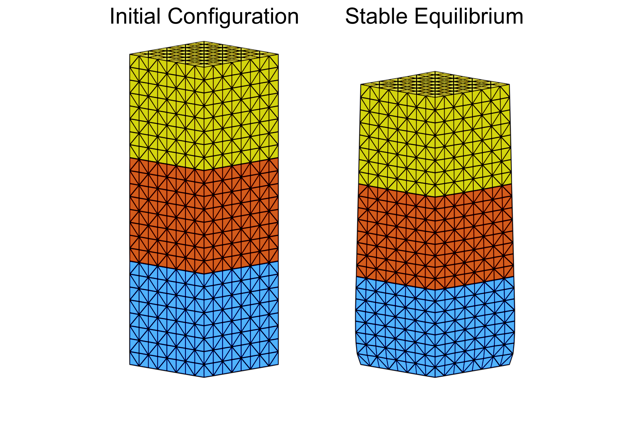
We study the static equilibrium of a stack of three blocks under refinement. We choose material parameters (, , and ) which are able to reach stable equilibrium without the stack falling yet produces a visible deformation (see fig. 17). Each block is , and we use five levels of refinement . We set and create an initial gap of . Additionally, we use friction with a coefficient of to prevent blocks from sliding off.
To solve for the static equilibrium we perform a series of incremental solves (time-stepping while zeroing out any velocity components at the start of every step). We perform this until convergence of the vertex positions (i.e. ). We choose a convergence tolerance of .
Figure 17 shows the results of this study where we see convergence of the center of mass, elastic energy, and contact pressure.
9.5 Dynamic Collision in 3D
We setup a two spheres colliding experiment to test the ability of our method to resolve elasticity and kinetic energy transfer caused by high-speed collisions. Two sphere meshes each with 29K nodes, wide are placed away from each other (fig. 18 a and b), both with Neo-Hookean elasticity, Young’s modulus , Poisson’s ratio and density , exactly the same material with the high-speed golf ball example in Li et al. [8], except that we do not apply any damping here. The two spheres are both with initial velocity towards each other. We set to (0.1% that of the sphere’s diameter) and to as usual. For stability and accuracy, we apply BDF-2 time integration at time step size .

During the simulation, the total x-direction momentum of the system is perfectly conserved with the the momentum of each sphere symmetrically and smoothly reversed (fig. 19 right). Since BDF-2 time integration is applied, the energy slightly dissipates around 10% of the initial total energy (fig. 19 left). But nice symmetry and coherence on the elasticity and kinetic energy profile of the two spheres are accurately resolved. With the energy data of the left and right spheres plotted as curve and dots respectively, it is clear that the curves are well-aligned. In fig. 18 c and d, we visualize the Von Mises stress on the spheres at a collision state and right after separation. Please see our supplemental video for the nice elastic wave propagation captured by our method.
9.6 3D Unit tests

The first unit test tests the ability of our method to handle tight conforming contacts. We drop a unit cube into a C-shaped slot. The slot is only wider than the cube. We use a soft material (, , and ) and a of with . We also utilize a framerate time step of . Our method passes this test without problem demonstrating the ability to handle small gaping and conforming contact.
Our second test positions two spikes such that they contact at the tips. This degenerate case is often challenging for traditional methods [3]. We use the same material parameters as the first unit test and set . Again we use a large . Our method has no difficulty in handling this contact, resolving the point-point contact into a downward diagonal motion.
9.7 Application: Microstructures
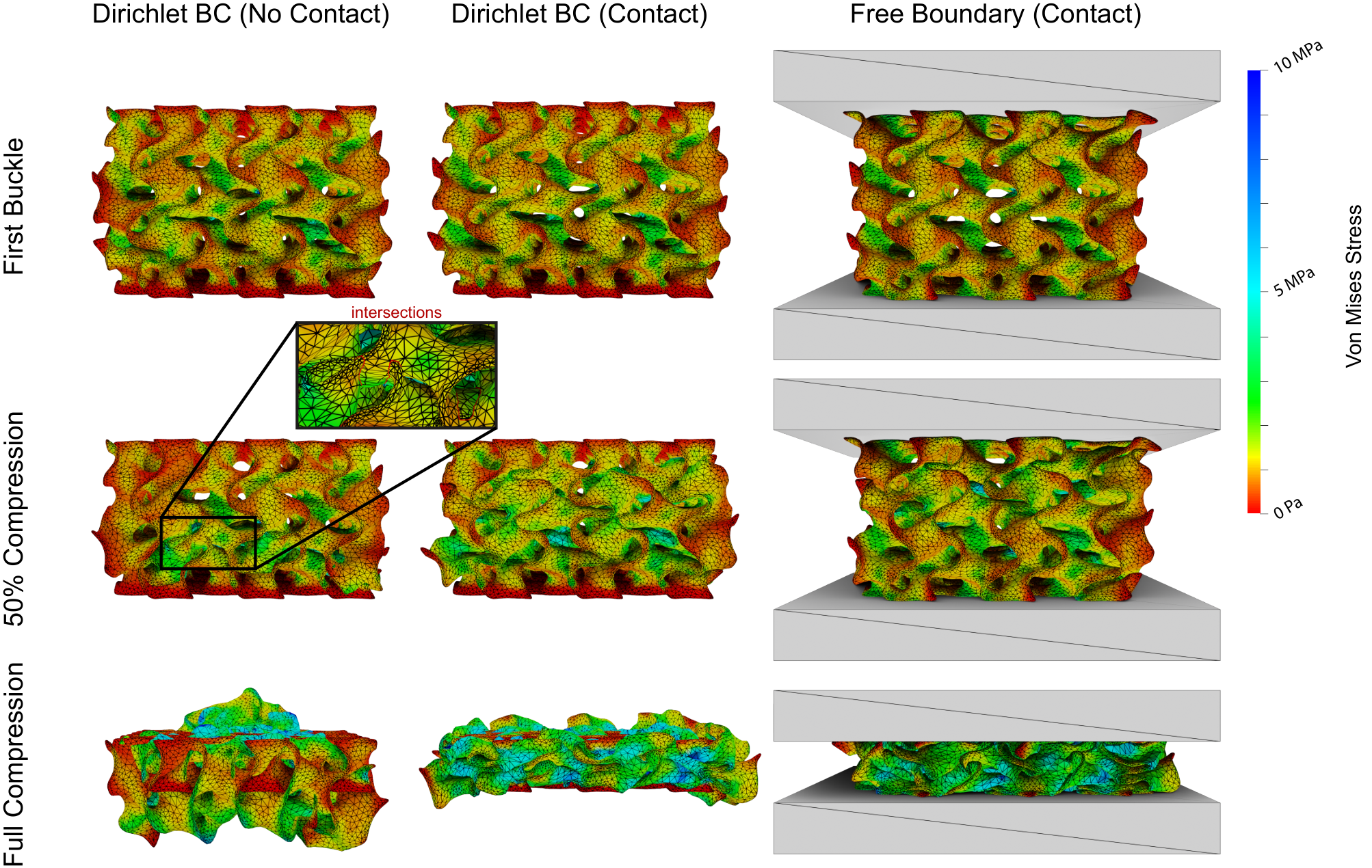

As an illustration of the importance of proper contact handling we apply our method to simulate the compression of a 3D printed gyroid micro-structure (fig. 21). We perform three simulations: (1) Dirichlet boundary conditions on the gyroid to compress it without contact resolution, (2) the same boundary conditions as (1) but now with contact modeled by our formulation, and (3) we apply the boundary conditions to rigid plates, leaving the gyroid’s boundaries free (again with contact). For the material parameters we match those of an 3D printed elastomeric polyurethane (, , and ). We plot the strain energy versus compression in fig. 22.
References
- [1] Y. Chen, M. Li, L. Lan, H. Su, Y. Yang, and C. Jiang, A unified newton barrier method for multibody dynamics, ACM Trans. Graph. (SIGGRAPH), 41 (2022).
- [2] D. Doyen, A. Ern, and S. Piperno, Time-integration schemes for the finite element dynamic signorini problem, SIAM Journal on Scientific Computing, 33 (2011), pp. 223–249.
- [3] K. Erleben, Methodology for assessing mesh-based contact point methods, ACM Transactions on Graphics, 37 (2018).
- [4] Z. Ferguson, M. Li, T. Schneider, F. Gil-Ureta, T. Langlois, C. Jiang, D. Zorin, D. M. Kaufman, and D. Panozzo, Intersection-free rigid body dynamics, ACM Transactions on Graphics (Proceedings of SIGGRAPH), 40 (2021).
- [5] C. Kane, J. E. Marsden, M. Ortiz, and M. West, Variational integrators and the newmark algorithm for conservative and dissipative mechanical systems, Int. J. for Numer. Meth. in Eng., 49 (2000).
- [6] L. Lan, D. M. Kaufman, M. Li, C. Jiang, and Y. Yang, Affine body dynamics: Fast, stable & intersection-free simulation of stiff materials, ACM Trans. Graph. (SIGGRAPH), 41 (2022).
- [7] L. Lan, Y. Yang, D. Kaufman, J. Yao, M. Li, and C. Jiang, Medial IPC: Accelerated incremental potential contact with medial elastics, ACM Transactions on Graphics (Proceedings of SIGGRAPH), 40 (2021).
- [8] M. Li, Z. Ferguson, T. Schneider, T. Langlois, D. Zorin, D. Panozzo, C. Jiang, and D. M. Kaufman, Incremental potential contact: Intersection- and inversion-free large deformation dynamics, ACM Transactions on Graphics (Proceedings of SIGGRAPH), 39 (2020).
- [9] M. Li, D. M. Kaufman, and C. Jiang, Codimensional incremental potential contact, ACM Transactions on Graphics (Proceedings of SIGGRAPH), 40 (2021).
- [10] X. Li, Y. Fang, M. Li, and C. Jiang, BFEMP: Interpenetration-free mpm–fem coupling with barrier contact, Computer Methods in Applied Mechanics and Engineering, 390 (2022), p. 114350.
- [11] X. Li, M. Li, and C. Jiang, Energetically consistent inelasticity for optimization time integration, ACM Trans. Graph. (SIGGRAPH), 41 (2022).
- [12] J. J. Moreau, On unilateral constraints, friction and plasticity, New Variational Tech. in Math. Phys., (1973).
- [13] J. Nocedal and S. Wright, Numerical optimization, Springer Science & Business Media, 2006.
- [14] M. Ortiz and L. Stainier, The variational formulation of viscoplastic constitutive updates, CMAME, 171 (1999).
- [15] J. Smith and S. Schaefer, Bijective parameterization with free boundaries, ACM Transactions on Graphics (Proceedings of SIGGRAPH), 34 (2015).
- [16] Y. Zhao, J. Choo, Y. Jiang, M. Li, C. Jiang, and K. Soga, A barrier method for frictional contact on embedded interfaces, Computer Methods in Applied Mechanics and Engineering, 393 (2022), p. 114820.