Robust and Resistant Regularized Covariance Matrices
Abstract
We introduce a class of regularized M-estimators of multivariate scatter and show, analogous to the popular spatial sign covariance matrix
(SSCM), that they possess high breakdown points. We also show that the SSCM can be viewed as an extreme member of this class.
Unlike the SSCM, this class of estimators takes into account the shape of the contours of the data cloud when down-weighing observations.
We also propose a median based cross validation criterion for selecting the tuning parameter for this class of regularized
M-estimators. This cross validation criterion helps assure the resulting tuned scatter estimator is a good fit to the data as well as having a
high breakdown point. A motivation for this new median based criterion is that when it is optimized over all possible scatter parameters, rather than
only over the tuned candidates, it results in a new high breakdown point affine equivariant multivariate scatter statistic.
Keywords: Breakdown point;
M-estimation; robust cross validation, multivariate shape; penalization; regularization; spatial sign covariance matrix.
1 Introduction
Though being the most efficient at normal distribution, the sample covariance matrix is well known to be non-robust in the sense that it is highly influenced by outliers and has relatively low efficiency at distributions which have longer tails than the multivariate normal distribution. A variety of of robust alternatives to the sample covariance matrix have been proposed, with the multivariate M-estimators [20, 13] being one of the earlier ones introduced. A drawback of the multivariate M-estimators, though, is they are not resistant, i.e. they have relatively low breakdown points in higher dimensions, specifically no greater than , with being the dimension of the data. Consequently, more resistant high-breakdown point estimators of scatter have been developed. These include the minimum volume ellipsoid (MVE) and minimum covariance determinant (MCD) estimators [26], S-estimators [2, 18], projection-based scatter estimators [4, 21], and MM-estimators [29].
All the above estimators are affine equivariant. For a -dimensional sample , a multivariate scatter statistic, say , is said to be affine equivariant if an affine transformation on the data , , induces the transformation on the scatter statistic , for and , the group of all nonsingular matrices.
As shown in [2], the finite sample contamination breakdown point of any affine equivariant scatter statistics is at most for any data set in general position, which is relatively low when is not much larger than . Furthermore, unlike the M-estimators, affine equivariant high breakdown point estimators tend to be computationally intensive, especially for large . They are typically computed via approximate or probabilistic algorithms. To handle these shortcomings, scatter estimators that sacrifice affine equivariance have been proposed, such as the spatial sign covariance matrix (SSCM) [17, 32]. The SSCM is an appealing candidate because of its simplicity. Not only does it have a high breakdown point regardless of , it is also computationally feasible for large .
The SSCM corresponds to a weighted covariance matrix for which the observations are downweighted relative to their Euclidean distance from the center of the data, regardless of the shape of the data cloud. In this paper, we show that a class of regularized M-estimators of scatter, which takes into account the shape of the data cloud in downweighing observations, can also have high breakdown points as well as be computationally feasible in high dimensions. The SSCM is shown to be an extreme member of this class of regularized scatter estimators, namely as a tuning parameter goes to its upper limit. The interpretation of the SSCM as a regularized M-estimator gives further insight as to why it performs best at spherical distributions, namely since it can be viewed as shrinking the scatter statistic towards proportionality to the identity. The broader class of regularized M-estimators of scatter can give improved performance when the true scatter matrix deviates from proportionality to the identity.
The class of regularized M-estimators of scatter only have a high breakdown points for a limited range of the tuning parameters. Also, within this class of estimators, there tends to be a trade-off between the breakdown point and how well the estimator can be used to fit the data. Nevertheless, we propose a robust median based cross validation criterion for selecting the tuning parameter which helps assure the resulting tuned scatter estimator is a good fit to the data while maintaining a breakdown point close to . A motivation for this new median based criterion is that when it is optimized over all possible scatter parameters, rather than only over the tuned candidates, it results in a new high breakdown point affine equivariant multivariate scatter statistic, see Remark 6.2.
The paper is organized as follows. We begin by reviewing the notion of the breakdown point, the definition and properties of elliptical distributions and of the spatial sign covariance matrix in Section 2. The definition and properties of penalized M-estimators of multivariate scatter are discussed in Section 3. The results on the breakdown points of these M-estimators for fixed tuning parameters are given in Section 4, wherein a new class of regularized M-estimators of scatter are also introduced. The trade-off between the breakdown point and bias when using fixed turning parameters is discussed in Section 5. A more detailed looked at tuning is given in Section 6 for the more specific class of distribution-free penalized and regularized M-estimators of scatter. This section also introduces and illustrates the median base cross validation method. Some concluding remarks are made in Section 7. All formal proofs are given in an appendix.
2 Preliminary concepts
2.1 Breakdown due to contamination
The breakdown point of an estimator represents a measure of its resistance to outliers in the data. Since its formal introduction in [12], a variety of definitions for the breakdown have been proposed. Here we use the concept of the finite sample contamination breakdown point, defined in [3, 5]. Roughly translated, this corresponds to the proportion of bad data in a sample that can be tolerated by an estimator before making the estimator arbitrarily bad. The formal definition is as follows.
Suppose the data set is contaminated by adding arbitrary data points . This produces an -contaminated sample consisting of a fraction of arbitrary bad values. Let represent a statistic, i.e. a function of the data. Next, define an unbounded bias function , which measures the discrepancy between and due to the contamination . For example, for a location statistic, a natural choice for the bias function is . For , the maximum bias at caused by -contamination is given by
| (1) |
where . Breakdown is said to occur under -contamination if . The finite sample contamination breakdown point of at is then defined to be
For a -dimensional scatter statistic , i.e. one whose range is the set of positive definite matrices, a natural choice for the bias function is the Riemannian metric . In this case, breakdown implies either the largest eigenvalue of can be arbitrarily large, the smallest eigenvalue of can be arbitrarily close to zero, or does not exist for some .
2.2 Elliptical distributions
A random vector is said to have an elliptical distribution if and only if it admits the representation , with having a uniform distribution on , being a univariate random variable independent of , , and being a fixed matrix. The distribution of depends on only through , and so we denote where . Standardizing gives a spherical distribution, i.e. for any orthogonal matrix , with the distribution of depending only on the radial distribution . This is denoted by .
For , if the first moments of exists then corresponds to the mean of , and if the second moments exist then is proportional to the covariance matrix of , with the constant of proportionality dependent only on . In general, whether or not the moments exist, refers to the center of symmetry and is referred to as the scatter matrix or pseudo-covariance matrix. Note that the definition of the scatter matrix is confounded with since . However, for an elliptical distribution the shape of , defined here as , is well defined. Furthermore, the shape of does not depend on and so can be view, together with as well defined parameters within the semi-parametric class of elliptical distributions, i.e. without being specified. In general, a shape matrix can be defined as any matrix of the form where is a positive scalar function such that . Another common choice is to take , see [23, 10], in which case the shape matrix then has determinant one rather than trace .
If is absolutely continuous, its density has spherical contours and is of the form , for some function , where refers to the Euclidean norm. The corresponding density of has concentric elliptical contours and is given by . For absolutely continuous cases, we denote and .
2.3 Spatial sign covariance matrix
In this section, we briefly review some properties of spatial sign covariance matrix. For more details, we refer the reader to [8], [19] and [32]. For , the spatial sign function is defined as with for and , where denotes the Euclidean norm in . The spatial sign corresponds to the unit vector in the direction of . The sample spatial sign covariance matrix is then defined as
where is the spatial median. Note that , and so corresponds to the sample covariance matrix computed from the spatial signs of the data. The SSCM is scale and location invariant and also orthogonally equivariant, i.e. the data transformation , induces the transformation , for any , and , the group of orthogonal matrices of order . The breakdown point of the SSCM is approximately . However, if is replaced with a fixed location , then the breakdown point becomes one, i.e. it cannot break down.
When the data represents a random sample from having distribution , then under mild conditions on the sample SSCM is strongly consistent for its functional or population value , where refers to expectation under the distribution , and is the population spatial median. When is an elliptical distribution with finite second moments, then the SSCM is known to have the same eigenvectors as those of the population covariance matrix, with the corresponding eigenvalues having the same order and multiplicities. However, as shown in [9], the eigenvalues of the population SSCM tend to be less separated than the eigenvalues of the population covariance matrix. Hence the SSCM can be viewed as shrinking the covariance matrix towards proportionality to the identity matrix.
This last property suggests that the SSCM may be related to penalized covariance methods. In the next section, we review the penalized M-estimators of multivariate scatter. Their relationship to the SSCM is discussed in Section 4.
3 Penalized M-estimators of multivariate scatter
When one has insufficient data, in that the sample size is small relative to the dimension of the data, regularization or penalization methods are natural to consider in order to obtain more stable estimators, see e.g. [16, 34]. In particular, a ridge approach for regularizing the sample covariance matrices is considered in [33], whereas the existence, uniqueness and computation of a regularized Tyler’s estimator is studied in [1, 24, 28]. Penalized versions of the M-estimators of multivariate scatter were proposed in [22], with special attention given to penalizing the trace of the precision matrix. For general penalties, the existence, uniqueness and computation of the penalized M-estimators of scatter are treated in [7].
Assume that the q-dimensional data has been robustly centered, e.g. by marginal medians or the spatial median, or by a known center. Alternatively, the data may be replaced with their pairwise differences. A penalized M-estimator of scatter is then defined as the matrix which minimizes,
| (2) |
over all , the set of positive definite symmetric matrices of order . Here , denotes a non-negative penalty function and is the penalty tuning parameter. For , (2) reduces to the objective or loss function associated with an M-estimator of scatter based on a given -function. Hereafter, we assume is continuously differentiable, and let , with the “influence function” being non-decreasing.
We first consider the trace precision matrix penalty , which has the effect of heavily penalizing when it is nearly singular. Properties of this penalty has been studied in [22, 33]. In particular, it is shown in [22] that, for any , any critical point of the penalized loss function (2) is a solution to the penalized M-estimating equation
| (3) |
Furthermore, if is bounded below, then (3) has a unique solution for regardless of the data set. When , i.e. an unpenalized M-estimator of scatter, it is known some conditions on the data set are needed to guarantee existence [15].
Similar results hold when using the Kullback-Leibler penalty function . Namely, the corresponding M-estimating equation is given by
| (4) |
where . Again, if is bounded below, then (4) has a unique solution for regardless of the data set.
If then, as with Tyler’s M-estimator [30], the resulting penalized M-estimator is distribution-free over the class of elliptical distributions. This follows since if then , the angular central Gaussian distribution with parameter , see e.g. [31], which does not depend on . However, the corresponding -function, given by , is not bounded below. For this special case, though, it is also shown in [22] that a unique solution to (3) exists regardless of the data whenever . By relating equations (4) to (3), we see that this statement also applies to (4) whenever . For other values of , some conditions on the sample are needed to ensure existence for these penalized Tyler’s M-estimators, see [22]. Since is not defined for , it is to be understood that when using the penalized Tyler’s M-estimators that the data set is replaced by the data set consisting only of the non-zero data points with corresponding sample size .
Remark 3.1.
The class of estimators defined via (3) and the class defined via (4) are essentially the same class of estimators. Suppose represents the solution to (3) with tuning parameter and weight function and represents the solution to (3) with tuning parameter and weight function then we have the relationship .
3.1 Scale equivariant versions of the scatter estimates
If we wish to pull the scatter estimator towards some rather than towards , then the penalty term can be replaced by . The resulting estimating equations (3) and (4) hold provided with and are replaced by and respectively. It is sufficient, though, to only consider the unaltered equations (3) and (4) since the results for general can be obtained by applying (3) or (4) to the transformed data set and noting .
The solutions to either (3) or (4) are not in general scale equivariant. That is, if for some , if we transform the data , , then the scatter estimator is not simply multiplied by . A scale equivariant scatter estimate can be obtained by choosing , with being an estimate of under the model such that the transformation , , induces the transformation . This is similar to the Ledoit-Wolf approach [16], which is based on pulling an unrestricted estimate of towards an estimate based on the model . In their case, they consider only the multivariate normal model and so pull the sample covariance matrix towards , with being maximum likelihood estimate of under the model . Rather than use we propose using a robust statistic such as , with being the spatial median. This choice of has a breakdown point of .
3.2 Computations
The penalized M-estimators of scatter and can be computed via simple re-weighing algorithms. Using the results for the fixed-point algorithm for finding the solution to (3) given in [22], it follows that given any initial starting value , the following algorithms
always converge to the unique solutions to (3) and (4) respectively. For the scale equivariant versions, the terms and in the algorithms are replaced by and respectively. More generally, if the penalty terms and are respectively replaced with and , then and in the algorithms are replaced by and respectively.
4 Breakdown point results
There appears to be little literature regarding the robustness properties of penalized M-estimators of multivariate scatter. In this section, we derive the finite sample contamination breakdown points of the estimator define by (3) and (4) above.
In the following, besides being continuously differentiable, we also presume it is non-decreasing and is either bounded below or . For the latter case, which corresponds to the penalized Tyler’s M-estimator of scatter, we further assume when working with (3) or when working with (4). These conditions assure (3) and (4) have unique solutions which we denote by and respectively. In general, besides being non-decreasing, we also presume it is bounded above and define . We then have the following result, which does not depend on how the data is centered. The matrix inequalities below refer to the partial ordering of symmetric matrices, i.e. if and only if . The proof of the following theorem is given in the appendix.
Theorem 4.1.
Under the stated assumptions on , regardless of the data ,
provided , and
provided . Hence, under these conditions, the estimators and cannot break down, i.e. when and respectively.
Remark 4.1.
The low breakdown point of the non-penalized M-estimates of scatter can be partially attributed to the possibility the estimate can be made to be arbitrarily close to a singular matrix under certain types of contaminations, see e.g. [6]. By contrast, the penalized M-estimators are obviously bounded away from singularity by construction, resulting in the left hand side of the inequalities in Theorem 4.1. In the following, we show that even if we adjust for this universal bound away from singularity, the resulting regularized estimators still retain high breakdown points.
We first focus on (4). Define , where denotes the solution to (4), and hence is the unique solution to the M-estimating equation
| (5) |
When , (5) corresponds to the usual M-estimating equations for a scatter matrix, provided a solution exists. On the other hand when , although , we have
which corresponds to a weighted covariance matrix with the data points being down-weighted based on their Euclidean distance from the center. These weighted covariance matrices have recently been studied in [27], wherein they are referred to as general spatial sign covariance matrices. Note that for one obtains the usual SSCM.
Consider now the solution to (3), denoted by , and define , which is the unique solution to the M-estimating equation:
| (6) |
When , this corresponds to the usual M-estimating equations for a scatter matrix, provided a solution exists. The relationship between (6) and the general SSCM is more involved. Suppose we consider the family of weight functions for a fixed function . Then, as , we have .
Rather than choose either extreme as one’s estimator, (5) and (6) provide classes of scatter estimators with tuning parameters and respectively. Moreover, the following theorem shows these adjusted regularized M-estimators have the same breakdown properties as the SSCM. The choice of the tuning parameter is discussed in a later section.
Theorem 4.2.
In addition to the stated assumptions on , suppose is also non-increasing. Let and , with and being defined as in Theorem 4.1. Furthermore, suppose the data spans , and is centered by a known or fixed center. Then,
- i)
for , provided .
- ii)
for , .
Remark 4.2.
If the data is centered by a location statistic having breakdown point , then it can be shown that under the conditions of Theorem 4.2 that .
Remark 4.3.
For the scale equivariant versions and , defined and , which are also scale equivariant. Under the conditions of Theorem 4.2, it can then be shown that .
Remark 4.4.
A more detail look at the breakdown point for general is discussed in Section 6 for the special case .
5 Bias versus breakdown considerations
Partially due to the simple relationship of to the general SSCM, we hereafter focus on the scatter statistics and , Analogous results for and can be obtained by using their relationship to and ; see Remark 3.1. Also, we drop the subscript for and and simply denote them as and .
When using robust estimators, a natural question to address is what is being estimated, and the general answer is the corresponding functional. For a given , the functional versions of and can be defined for the former as the solution to the matrix equation
| (7) |
where is a random vector with distribution . Again, we assume the function satisfies the conditions discussed in Section 3, which assures (7) has a unique solution. The functional version of is then given by .
For a parametric class of distributions, the functionals themselves can be expressed in terms of the parameters. For elliptical distributions, the following theorem establishes an important property and share with the functional version of the SSCM, namely they have have the same eigenvectors as as well as the same ordering and multiplicities of their eigenvalues.
Theorem 5.1.
For and with being non-increasing, the matrices , and can be simultaneously diagonalized, i.e. for some orthogonal matrix ,
where and , with and . Also, , with . Furthermore, for , , and if then and .
The elements of , and hence of , are strictly functions of the elements of . In particular, as shown within the proof of Theorem 5.1, is the unique solution to the system of equations
| (8) |
where .
So, as with the SSCM, the eigenvector of the regularized M-estimators and , for a given , are Fisher consistent for the eigenvectors of , but not necessarily for the corresponding eigenvalues. As shown in [9], the eigenvalues of the SSCM functional are less dispersed than those of , i.e. the SSCM is closer to being proportional to the identity matrix than . The following theorem, which uses the notation of Theorem 5.1, shows that this is also the case in general for and for .
Theorem 5.2.
Suppose with being decreasing. Also, in addition to the stated assumptions on , suppose is non-increasing. For , if , then for ,
Furthermore, is a decreasing function of , with when and when .
This theorem states that the ratio of any two eigenvalues of are closer to one than the corresponding ratio of the eigenvalues of which in turn are closer to one than the corresponding ratio of the eigenvalues of the population scatter matrix , or equivalently of the population shape matrix . From Theorem 5.2, it follows , and under a sequence of values for , if then . In general, though, the values of and can greatly differ. This is demonstrated in Table 1 below.
Table 1 gives the values of the condition numbers , and when using the weight function . When , this weight function corresponds to the weight function arising from the maximum likelihood estimator for an elliptical t-distribution on 2 degrees of freedom. The values of are obtained by solving (8), with the expectation evaluated by using a Monte Carlo simulation based on a sample size of . The values of the condition numbers are evaluated under the multivariate normal distribution. In the table, slightly exceeds for the case , and , which seems to contradict Theorem 5.2. However, this is an artifact of the simulations since the condition number is a convex function and tends to be overestimated in a simulation.
| 0.05 | 0.20 | 0.50 | 0.80 | 0.95 | 0.05 | 0.20 | 0.50 | 0.80 | 0.95 | ||
|---|---|---|---|---|---|---|---|---|---|---|---|
| 0.5 | 1.22 | 1.17 | 1.09 | 1.03 | 1.00 | 4.91 | 5.03 | 5.19 | 5.30 | 5.35 | |
| Model 1 | 1 | 1.53 | 1.40 | 1.21 | 1.07 | 1.01 | 5.37 | 5.39 | 5.39 | 5.38 | 5.37 |
| 3 | 4.00 | 2.92 | 1.81 | 1.24 | 1.05 | 7.65 | 7.09 | 6.29 | 5.68 | 5.44 | |
| q = 5 | 5 | 7.38 | 5.03 | 2.66 | 1.43 | 1.08 | 9.31 | 8.49 | 7.20 | 6.01 | 5.51 |
| 8 | 9.38 | 7.43 | 4.12 | 1.79 | 1.14 | 9.94 | 9.49 | 8.27 | 6.51 | 5.62 | |
| 0.5 | 1.13 | 1.11 | 1.06 | 1.02 | 1.00 | 5.91 | 5.99 | 6.12 | 6.22 | 6.26 | |
| Model 2 | 1 | 1.31 | 1.24 | 1.13 | 1.04 | 1.01 | 6.10 | 6.15 | 6.22 | 6.26 | 6.27 |
| 3 | 2.66 | 2.11 | 1.50 | 1.15 | 1.03 | 7.22 | 6.98 | 6.65 | 6.41 | 6.31 | |
| q = 5 | 5 | 6.36 | 3.87 | 2.04 | 1.28 | 1.06 | 8.99 | 8.10 | 7.16 | 6.57 | 6.34 |
| 8 | 9.33 | 7.03 | 3.27 | 1.51 | 1.10 | 9.92 | 9.38 | 8.01 | 6.83 | 6.40 | |
| 0.5 | 1.05 | 1.04 | 1.03 | 1.01 | 1.00 | 8.08 | 8.08 | 8.07 | 8.07 | 8.07 | |
| Model 1 | 2 | 1.24 | 1.20 | 1.12 | 1.04 | 1.01 | 8.31 | 8.27 | 8.20 | 8.12 | 8.08 |
| 20 | 4.16 | 3.57 | 2.49 | 1.53 | 1.12 | 9.57 | 9.46 | 9.15 | 8.63 | 8.23 | |
| q = 50 | 50 | 7.67 | 6.43 | 4.19 | 2.14 | 1.25 | 9.94 | 9.86 | 9.60 | 9.01 | 8.38 |
| 53 | 9.57 | 8.14 | 5.30 | 2.56 | 1.33 | 10.04 | 9.97 | 9.75 | 9.19 | 8.47 | |
| 0.5 | 1.01 | 1.01 | 1.00 | 1.00 | 1.00 | 9.43 | 9.43 | 9.44 | 9.44 | 9.44 | |
| Model 2 | 2 | 1.06 | 1.05 | 1.03 | 1.01 | 1.00 | 9.45 | 9.45 | 9.44 | 9.44 | 9.44 |
| 20 | 1.96 | 1.74 | 1.39 | 1.13 | 1.03 | 9.60 | 9.58 | 9.52 | 9.47 | 9.45 | |
| q = 50 | 50 | 4.74 | 3.45 | 2.03 | 1.30 | 1.06 | 9.82 | 9.74 | 9.61 | 9.51 | 9.45 |
| 53 | 9.22 | 5.86 | 2.66 | 1.42 | 1.08 | 10.03 | 9.88 | 9.68 | 9.53 | 9.46 | |
This implies, for any fixed , the estimators and can be heavily biased estimates of the population scatter matrix. This is also true for the corresponding estimates of the population shape matrix. This bias is partially due to the nature of penalization, i.e. a trade off is made to obtain a less variable or more stable estimator, especially for smaller sample sizes, at the expense of generating more bias at some models. Typically, when using penalization methods, the bias tends to be fairly small whenever the tuning parameter is close to zero and the sample size is large. As seen in Table 1 , though, the bias can still be quite extreme in such cases, especially when considering the higher breakdown point estimates. Due to this large universal bias over , any method used to choose the tuning parameter , such as cross-validation, would still result in a heavily biased estimator regardless of the sample size.
To help understand the nature of this bias, recall that when the M-estimating equations (4) and (5) reduce to the
non-penalized M-estimating equations for multivariate scatter. It is known, though, that a necessary condition for existence of a solution in the
non-penalized case is . However, the condition needed for Theorems 4.1 and 4.2 does not
hold whenever unless is fairly large, namely . So, for , if is bounded below then although
and exist and are unique for any their limits do not exist as . Due to this
discontinuity, their bias does not necessarily get small as for a fixed . One could greatly reduce the bias, by choosing a weight
function for which , but this would result in a relatively low breakdown point. For general , resolving this trade-off between
bias and breakdown is a rather formidable problem and we leave it for a future study. Due to some properties associated with the special case
, though, we are able to propose a resolution for this special case in the next section.
6 The distribution-free regularized M-estimates of scatter
In this section we consider the special case based on Tyler’s weight function . As noted in Section 3, the distribution of the resulting regularized estimates do not depend on from which elliptical family the data arises. Another interesting aspect of this class of estimates is that its corresponding shape matrix is the same whether or not one uses a scale invariant version of the penalized estimate as defined in Section 3.1. That is, if we define to be the unique solution to
| (9) |
then , and so their respective shape matrices and are equal. The shape matrix for also does not depend on .
To obtain a compromise between bias and breakdown for the regularized M-estimates of scatter estimate, there are two tuning parameters to consider, namely and . When tuning for the shape matrix using Tyler’s weight function, the problem can be reduced to the single parameter . This follows, since as observed in [22], for , if we let denote the unique solution to
| (10) |
then for any two values and , . Also, for , we have the relationship . Consequently, the shape matrices and do not depend on the value of .
As noted in Section 3, some conditions on the sample are needed to ensure (10) admits a unique solution. These conditions, given by Condition A in [22], place some restrictions on how many data points can lie within subspaces. Specifically, the inequaltiy must hold for any subspace of . This condition always holds when . When the data are in general position, i.e. when every subset of data points spans a subspace of dimension , the condition holds for any . When randomly sampling from a continuous distribution in , the data are in general position with probability one.
Using the results on existence, we can extend the breakdown point results given in Section 4. The proof of the following theorem is given in the appendix.
Theorem 6.1.
Suppose for and for . If the sample is in general position, then
- i)
for , and
- ii)
for as .
The above breakdown points hold for a fixed , but do not necessarily apply when is determined by the data. As noted in the forthcoming section, it is possible for the data driven choice of to be close to and the resulting tuned scatter matrix to have a high breakdown point.
Remark 6.1.
As noted above, neither nor depend on the value of . The value of only affects the scale of the scatter matrix. Rather than let determine the scale, an alternative to is to define , where . The scatter statistic can be defined analogously. Here both and are scale invariant, whereas and are scale equivariant, i.e. for any . The values of contribute to the value of , whereas they do not contribute to the value of the shape statistics . Although the shape statistics are distribution free under random samples from elliptical distributions, the distribution of would be dependent on the specific elliptical distribution.
6.1 Choosing the tuning parameter
Oracle methods for choosing tuning parameters for variants of the regularized distribution-free M-estimators of scatter have been proposed in the literature, see e.g. [1, 22]. It is not clear, though, how severely the final tuned estimators are affected by outliers. In this section, we focus on the shape matrix, which is well defined within the semi-parametric class of elliptical distributions, and consider a more data dependent approach to tuning, namely cross-validation over . In deciding on a value of , the resulting estimate of shape or should be a good fit to the data. We consider as a cross-validation criterion the negative log-likelihood associated with the angular central Gaussian distribution [31], which for a subsample is given by
| (11) |
where is an estimate of or based on a subsample of size not containing . Observe that for any , and so the function only depend on through its shape matrix . Also, the value is invariant under multiplication of the data points by constants, i.e. under the transformation for any set of constants .
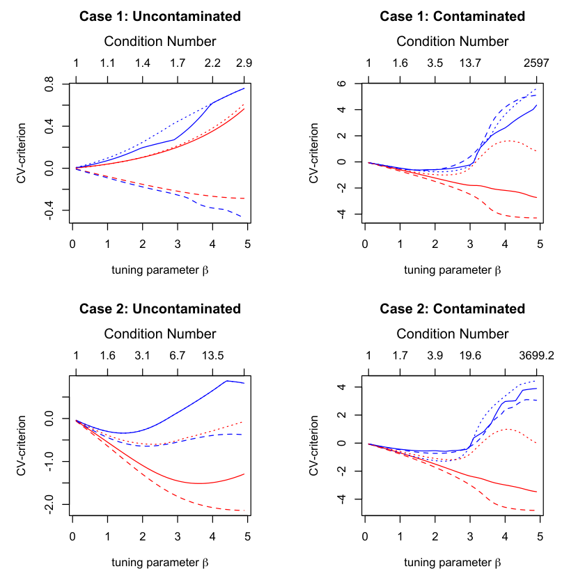
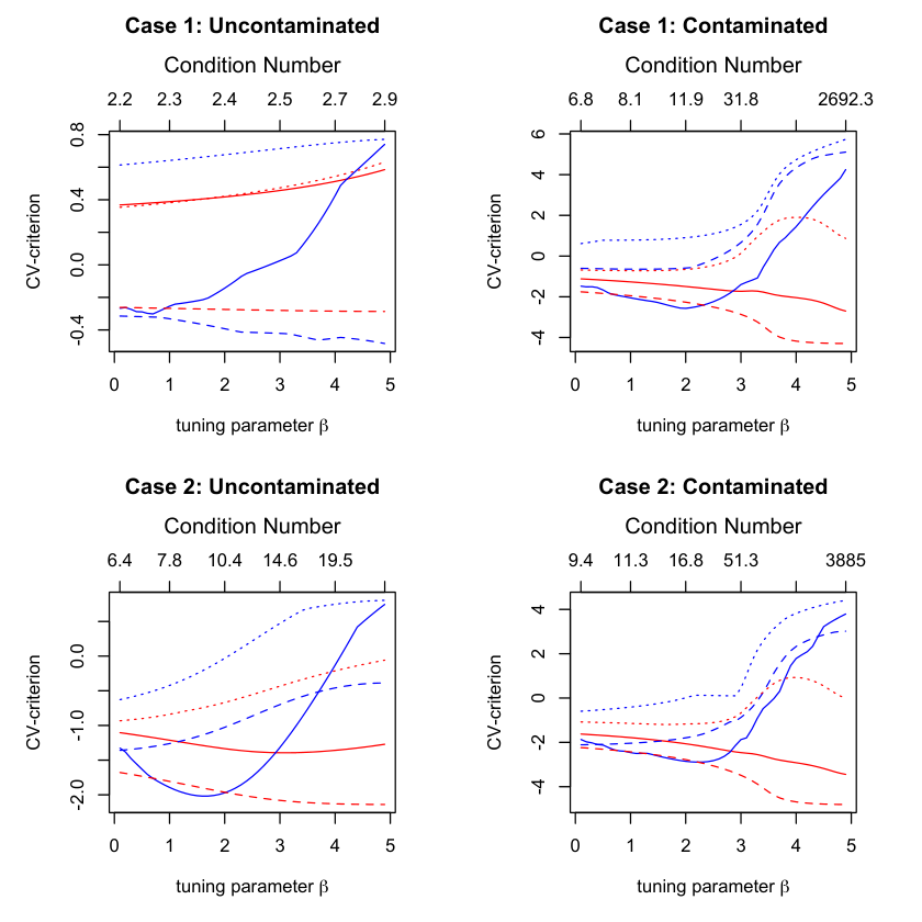
Figures 1 and 2 illustrates the use of 5-fold cross validation over for and respectively, with the grid for being in increments of . The top axes gives the condition number for the given value of . Cases 1 and 2 correspond to random samples of size from a dimensional multivariate normal distribution with mean zero and respective covariance matrices and , and so the corresponding condition numbers are 1 and 10. The contaminated cases in the figures are generated by randomly replacing of the good observations with the symmetric contaminating points , with being a random sample from a dimensional multivariate normal distribution with mean and covariance matrix . The proportion of contamination is thus or . The cross validation curves in Figures 1 and 2 given by the average of (11) over the five validation subsamples is denoted as the cvmean criterion and is represented by the solid red lines in the figures. For the uncontaminated case 1, the minimum is obtain at for both and , i.e. the perfect estimate and the SSCM respectively. For the uncontaminated case 2, the minimum for is obtain at and for at . For these two cases, the estimates seems reasonable, with the estimate based on being better than that based on . For the contaminated cases, though, the minimum is always obtained at with , i.e. the estimates break down.
CROSS VALIDATION METHODS APPLIED TO
CROSS VALIDATION METHODS APPLIED TO
Besides providing a good fit to the data when the data is not contaminated, another consideration when deciding on a value of is that the resulting estimate of shape should have good breakdown properties, say does not breakdown under contamination. This implies that the condition number should be bounded above under contamination. From Theorem 6.1, a breakdown point of at least can be obtained if we restrict cross validation to . However, this may not necessarily yield an estimate which is a good fit to the data when little or no contamination is present, especially for large . We therefore propose the following alternative approach.
When the data is contaminated, the cross validation criterion measures how well a shape matrix fits the contaminated data set, i.e. the mixture of the good and bad data points. As noted in [25], outliers may place undue influence on the chosen model or in our case the chosen value of . To place more weight on how well the good data are fitted, we propose replacing the average in 11 with the median to obtain the more robust criterion
| (12) |
Note that other measures of center besides the average and the median could also be considered in defining the cross validation criteria. A similar concept has been proposed in the context of ridge regression in [14]. Analogous to the criterion , this criterion also depends only on the shape matrix , and is invariant under multiplication of the data points by constants.
A motivation for considering (12) is to observe that the value of which minimizes (11) for the full data set, i.e. , corresponds to Tyler’s distribution-free M-estimate of scatter which has a breakdown point of . However, as shown in Theorem 6.2 below, the breakdown point of goes to as . We wish to emphasize that the estimate introduced here corresponds to a new affine equivariant high breakdown point scatter statistic, see Remark 6.2. Although is known to be readily computed via a simple reweighing algorithm, the statistic , as is common with all affine equivariant high breakdown point scatter statistics, appears to be computationally intensive. However, we do not need to compute for our purposes. Rather, we only need to minimize over the candidate values of .
In K-fold cross validation, some subsamples obtained from the partitioning may contain over 50% bad data points when the data is highly contaminated. So, rather than taking the average of over the K validation subsamples, we propose either replacing the average with the median, and i.e. taking the median of the medians, or to simply use
| (13) |
i.e. the median over all such values arising in (12) from the K validation subsamples. These different cross validation approaches are also illustrated in Figures 1 and 2. The cross validation curves obtained using (13) is denoted the cvmed criterion and is represented by the solid blue lines in the figures, whereas those associates with taking the mean and median of (12) over the five validation subsamples are denoted the cvmedmean and the cvmedmed criterion respectively, and are represented by the dotted red and the dotted blue lines in the figures. The dotted blue line coincides with the solid blue line in Figure 1 in the uncontaminated case 2.
For the uncontaminated case 1, the minimum is again obtain at for any of the above criterion, with the exception of cvmed for for which the minimum is obtained at . So, all of the estimates based on the four different cross validation criterion give comparable results for this case. For the uncontaminated case 2, the minima for are obtained at , and for cvmed, cvmedmean and cvmedmed respectively, and the minima for are respectively obtained at , and . For this case, the estimates based on the robust cross validation criterion are comparable to the estimates based on the cvmean, with the exception that the error in the condition number for is smallest for the criterion cvmean, whereas for it is smallest for the criterion cvmed. Overall, the robust cross validation criterion appears to be minimized at smaller values of than cvmean, i.e. they tend to more heavily shrink the estimate towards proportionality to the identity.
For the contaminated cases, though, we see that the estimates based on the robust cross validation criterion do not breakdown. Also, the errors in the the estimated condition numbers are not too large even under close to contamination. In particular, the minima for based on cvmed, cvmedmean and cvmedmed respectively are , and for contaminated case 1 and , and for contaminated case 2. The corresponding values for are , and for contaminated case 1 and , and for contaminated case 2. One can note that for the contaminated cases, the curves associated with cvmeanmed tend to curve downward for larger values of , although not enough to cause breakdown since the minima are not obtained at the upper extreme. Also, the curves for cvmed tend to be less smooth than the other curves. Based upon these limited results, we believe cvmedmed to be the best criterion to use for cross validation. It is also interesting to note that the robust cross validation curves for the contaminated cases tend to sharply increase near . This agrees with Theorem 6.1 which states that the breakdown point at is approximately , whereas the proportion of contamination is , and suggests the robust cross-validation curves may help ascertain the approximate percentage of the data which may be contaminated.
Another method for choosing the tuning parameter without using cross validation is to simply minimize the robust cross-validation criterion (12) over without using subsamples. That is, define
| (14) |
with the resulting tuned penalized shape matrix then being , or when is replaced by in (14). Choosing the tuning parameter in this manner requires less computations than cross validation methods. Also, as noted in Theorem 6.2 below, the breakdown point of the resulting tuned shape matrix is approximately for large .
Theorem 6.2.
If is in general position, then the finite sample contamination breakdown point for , where is either , or , satisfies
Obtaining exact results for the breakdown point for the shape estimates based on , the value of obtain via cross validation, is a more challenging problem due to the randomness of arising from the simulated partitioning of the data. We leave this as an open problem, although based on Figures 1 and 2 we conjecture that the breakdown points will be near when using the median based cross validation methods,
The behavior of the criterion , denoted as acgmed and represented by a dashed blue curve, is also illustrated in Figures 1 and 2. For completeness we also include in the figures the criterion which is denoted by acgmean and represented by the dashed red curve. Note that the acgmean curve is always minimized at since as previously noted which minimizes over all . The acgmed curve is also minimized when for both and for the uncontaminated case 1. For the other cases, acgmed curve tends to have properties similar to the cvmedmed curve, which suggests its use may provide a computationally simpler viable estimate, especially for large sample sizes and/or high dimensions. In particular, for the uncontaminated case 2, the acgmed curves in Figures 1 and 2 are minimized at and respectively. For the contaminated cases, the curves for case 1 are respectively minimized at and and those for case 2 are minimized at and .
Remark 6.2.
The shape statistic is equivariant under linear transformations of the data in the sense that if is non-singular, then . If we define the scatter statistic , where , then it satisfies . The breakdown point for is the same as the breakdown point for given in Theorem 6.2.
Using a technique introduced in Kent and Tyler (1991), one can generate an affine equivariant multivariate location and scatter statistic by appending a one to each observation in , that it define where , and then partition
The resulting statistics are high breakdown point affine equivariant multivariate location and scatter statistics.
7 Concluding remarks and future directions
A motivation for considering the regularized M-estimators of scatter is to observe that the SSCM does not take into account the shape of the data cloud when down-weighing observations, but rather down-weights based on their Euclidean distances from the center. On the other hand, the non-penalized M-estimators down-weights observations based on their adaptive Mahalanobis distances. However, in addition to their relatively low breakdown points in higher dimension, these M-estimators may be ill-conditioned when the sample size is of the same order as the dimension of the data. The regularized M-estimators of scatter can be seen as a compromise between these approaches to down-weighing observations. They take into account the shape of the data cloud, but adjust the Mahalanobis contours towards a more spherical shape. This helps prevent problems which may arise from inverting an ill-conditioned scatter matrix. Overall our proposed method has ease of computation and the stability of an M-estimate while being a high breakdown method resistant to outliers.
Although the emphasis on tuning in this paper is on the distribution-free regularized M-estimators of shape, the cross-validation (11) and the robust cross-validation (12) criteria for shape can be used for regularized M-estimators in general. In this more general case, cross validation needs to be done over the parameters and . Here, the parameter can be defined within a class of weight functions , with being a fixed function with and hence . The idea is to still focus on the shape of the scatter functional, which is well defined within the semi-parametric class of elliptical distributions. Rather than use the scale associated with or , we again propose defining scale as in Remark 6.1. For example, given the estimate for shape , define the regularized estimate of scatter as where , with the constant is customarily chosen so that is consistent at the multivariate normal model. Also, we believe the breakdown point results given Theorem 6.1 can be extended to general weight functions and in particular we conjecture for this more general setting that the breakdown point is approximately .
The high breakdown point estimator discussed in Remark 6.2 is a special case of a maximum trimmed likelihood estimator (MTLE), or more specifically a maximum median likelihood estimator (MMLE), as defined in [11]. In particular, the estimator is the MMLE under the angular central Gaussian distribution, which can be viewed as being at the extreme end of elliptical distributions. A general class of cross-validation criteria can be constructed using the objective function associated with an MTLE or MMLE for other elliptical distributions, and their properties would be worth exploring in future research. It is worth noting that it is shown in [11] the MMLE under the multivariate normal model is the MVE. As emphasize in our paper, using the angular central Gaussian model has the advantage of depending only on the well-defined shape matrix of the elliptical distribution, as well as being distribution-free over the class of elliptical distributions.
Finally, we note that a an R-package is being developed to implement the methods proposed in this paper, and that a large simulation study for the tuned regularized M-estimates of scatter is on-going and will be reported elsewhere.
Acknowledgements
Research for David E. Tyler’s and Mengxi Yi was supported in part by National Science Foundation Grants DMS-1407751
and DMS-1812198. Mengxi Yi’s research was also supported in part through Austrian Science Fund (FWF) under grant P31881-N32, the
National Natural Science Foundation of China (No. 12101119) and the Fundamental Research Funds for the Central Universities
(310422113).
Appendix: Proofs
Proof of Theorem 4.1
Proof of Theorem 4.2
Consider the contaminated data set , where . For this data set, denote the solution to (6) by , and let be the smallest eigenvalue of . Since
it follows from the non-increasing property of the weight function that
Thus, from (6) we obtain
Therefore, is bounded below over all possible contaminations as long as the good data spans . By Theorem 4.1 it follows that is also bounded above over all . Hence it cannot break down. The proof for is analogous.
Proof of Theorem 5.1
Part a: We first show that the matrices and are jointly diagonalizable. That is, they possess the same eigenvectors. To prove this, let . Pre- and post-multiplying (7) by gives:
| (15) |
Denote the spectral value decomposition of . Since , pre- and post-multiplying (15) by and respectively gives:
| (16) |
where . Since the distribution of is invariant under sign changes of its components, mapping implies
Hence, the matrix is diagonal. Since is also diagonal by
definition, it follows that must be diagonal and consequently the spectral value decomposition of is given
by . Also, , where .
Hence, the columns of correspond to both the eigenvectors of and the eigenvectors of .
Part b: The formula for given in (8) follows by pre- and post-multiply (16) by and then extracting the diagonal elements. It is convenient for the following proofs to express (8) as
| (17) |
where and .
Part c: Next, we show the eigenvalues associated with the eigenvectors of and have the same order. That is, for and , . We also show . If , then this result readily follows. Thus, we only need to consider the case for which . For this case, we show , and so it follows that or . To show , recall is increasing and is decreasing in , and so is increasing and is decreasing in when holding fixed for . Also, is strictly increasing in when holding fixed for . This implies
where with . is defined as in (18). Finally, since for any permuation , we obtain
Part d: Finally, we show the multiplicities of the eigenvalues of and are the same. That is, . Suppose , then
| (18) |
where and is defined as above. Since for any orthogonal of order , it follows that can be replaced by in (18). However, we know that and hence is uniquely defined, and so for any orthogonal , which implies or . The other direction, i.e. , follows from the result that if then , which is established above. So, if but , then either or , depending on whether or respectively, a contradiction. Hence, .
Proof of Theorem 5.2
If , then and so it readily follows
So, we only need to prove strict inequality holds when , which we hereafter assume holds.
Part a: We first note that is strictly increasing in on . Thus,
.
Part b: Next, we show , which is equivalent to
. Since , it follows that , where is defined as in (17). It was shown within Part c of the proof of Theorem 5.1 that . Analogous arguments give , a contradiction. Hence
.
Part c: Finally, we show , which is equivalent to showing . From (8), with , we have
So showing is equivalent to showing . To do so, recall that the distribution of is invariant under permutations. This gives the identity
| (19) |
where and
It was established in Part b that and so on . Since is a decreasing function,
it follows that the right hand side of (19) is positive and hence .
Proof of Theorem 6.1
The case has already been considered in detail in Section 4. Consider the case . For and , we first show under the conditions of the theorem that exists. By condition A in [22], existence is assured if holds for any subspace of . Since is in general position, at most sample points from can lie in . This implies that at most elements of lies in . Now holds for if it holds for , i.e. exists if or .
To complete the proof, we show that for the largest and smallest eigenvalues of are bounded above and away from zero respectively, i.e. that can not breakdown under contamination. Now where where for , with being a compact set. So if breakdown occurs when then there exists sequence for which the largest eigenvalue of goes to infinity and/or its smallest eigenvalue goes to zero. However, since is a continuous function of , this contradicts , and hence breakdown cannot occur. The results for follows after noting that it can only be non-singular when .
Proof of Theorem 6.2
For and , define
| (20) |
Since for any and , we can presume without loss of generality that is on the unit sphere , and , where are the eigenvalues of . In general, for a sequence , express their spectral value decompositions as , where with being the eigenvalues of , and being orthogonal matrices whose columns are normalized eigenvectors of , with for .
Lemma A.1.
Let be a sequence in , and let be a sequence such that and as . If the sequence bounded away from zero for large enough , then .
Proof.
Express , where
. Since , is bounded below and
as , it follows that
∎
For the sample and , define
| (21) |
Lemma A.2.
Suppose the fixed sample is in general position, and is an arbitrary sample. For a sequence with , if then .
Proof.
For any , it follows from Lemma A.1 that unless there is a sequence in such that as . Since lies in a compact set, it can be assumed that and so if holds, then . Since is in general position, holds for at most element of . This implies for at least sample points in . The result then follows since consist of sample points. ∎
For the sample , we can express , provided the infimum exists. If the infimum exists and is achieved at , then it is also achieved at for any . All such solutions give the same value for . It may be possible though for to not be well defined since the global minimum above may not be unique up to scalar multiplication. In such an unlikely case, can be taken to be the average of all such values. Conditions for the existence of are given in the following lemma.
Lemma A.3.
Let and be defined as in Lemma A.2 with . For a given , is bounded below over . Furthermore, exists and .
Proof.
In general . So, if is not bounded below then there exists a sequence such that . This implies or equivalently . However, Lemma A.2 then states , a contradiction. Now, since is also continuous over , it follows exists. Finally, if , then Lemma A.2 is again contradicted. ∎
The breakdown point for given in Theorem 6.2 is an immediate consequence of Lemmas A.2 and A.3, since for , exist with its largest eigenvalue equal to by definition and its smallest eigenvalue bounded away from zero for all . The breakdown points of and also follows since under and for we know they exist and their largest eigenvalues are again equal to . Finally, we know that under and for their smallest eigenvalue is bounded away from zero over all . Otherwise would not be bounded above for all which contradicts the breakdown point being one for any .
References
- [1] Chen, Y., Wiesel, A., and Hero, O.A. (2011) Robust shrinkage estimation of high-dimensional covariance matrices. IEEE Transactions on Signal Processing, 59, 4097-4107.
- [2] Davies, L. (1987). Asymptotic behavior of S-estimators of multivariate location parameters and dispersion matrices. The Annals of Statistics, 15, 1269-1292
- [3] Donoho, D. (1982). Breakdown properties of multivariate location estimators. Ph.D. Qaulifying Paper, Harvard University.
- [4] Donoho, D., and Gasko, M. (1992). Breakdown properties of location estimates based on halfspace depth and projected outlyingness. The Annals of Statistics, 20, 1803-1827.
- [5] Donoho, D., and Huber, P. (1983). The notion of breakdown point. In: A Festschrift for Erich L. Lehmann, (P.J. Bickel, K. Doksum and J.L. Hodges, Jr., Eds.), Wadsworth, Belmont, CA, 157–184.
- [6] Dümbgen, L. and Tyler, D.E. (2005). On the breakdown properties of some multivariate M-functionals. Scandinavian Journal of Statistics, 32, 247-264.
- [7] Dümbgen, L. and Tyler, D.E. (2016). Geodesic convexity and regularized scatter estimators. arXiv:1607.05455v2 [stat.ME].
- [8] Dürre, A., Vogel, D., and Tyler, D. E. (2014). The spatial sign covariance matrix with unknown location. Journal of Multivariate Analysis, 130, 107-117.
- [9] Dürre, A., Vogel, D., and Tyler, D. E. (2016). On the eigenvalues of the spatial sign covariance matrix in more than two dimensions. Statistics & Probability Letters, 111, 80-85.
- [10] Frahm, G. (2009). Asymptotic distributions of robust shape matrices and scales. Journal of Multivariate Analysis, 100, 1329-1337.
- [11] Hadi, A.S. and Ludeño, A. (1997) Maximum trimmed likelihood estimators: a unified approach, examples, and algorithms. Computational Statistics & Data Analysis, 25, 251-272.
- [12] Hampel, F. R. (1971). A general qualitative definition of robustness. The Annals of Mathematical Statistics, 42, 1887-1896.
- [13] Huber, P. J. (1977). Robust covariances. In: Statistical decision theory and related topics II, (S.S. Gupta & D.S. Moore, Eds.), Academic Press, New York, pp. 165-191.
- [14] Jung, K.-M. (1991). Robust cross validations in ridge regression. Journal of Applied Mathematics & Informatics, 27, 903-908.
- [15] Kent, K.T. and Tyler, D.E. (1991). Redescending M-estimates of multivariate location and scatter. The Annals of Statistics, 19, 2102-2119.
- [16] Ledoit, O. and Wolf, M. (2004). A well-conditioned estimator for large dimensional covariance matrices. Journal of Multivariate Analysis, 88, 365–411.
- [17] Locantore, N., Marron, J.S., Simpson, D.G., Tripoli,N., Zhang, J.T. and Cohen, K.L. (1989). Robust principal components for functional data. Test, 8, 1-28.
- [18] Lopuhaa, H. P. (1989). On the relation between S-estimators and M-estimators of multivariate location and covariance. The Annals of Statistics, 17, 1662-1683.
- [19] Magyar, A. F., and Tyler, D. E. (2014). The asymptotic inadmissibility of the spatial sign covariance matrix for elliptically symmetric distributions. Biometrika, 101, 673-688.
- [20] Maronna, R. (1976). Robust M-estimators of multivariate location and scatter. The Annals of Statistics, 4, 51-67.
- [21] Maronna, R. A., Stahel, W. A., and Yohai, V. J. (1992). Bias-robust estimators of multivariate scatter based on projections. Journal of Multivariate Analysis, 42, 141-161.
- [22] Ollila, E. and Tyler, D.E. (2014). Regularized M-estimators of scatter matrix. IEEE Transactions on Signal Processing, 62, 6059-6070.
- [23] Paindaveine, Davy, (2008). A canonical definition of shape. Statistics & Probability Letters, 78, 2240-2247.
- [24] Pascal, F., Chitour, Y. and Quek, Y. (2014). Generalized robust shrinkage estimator and its application to STAP detection problem. IEEE Transactions on Signal Processing, 62, 5640-5651.
- [25] Ronchetti, E., Field, C. and Blanchard, W.(1997). Robust linear model selection by cross-validation. Journal of the American Statistical Association, 92, 1017-1023
- [26] Rousseeuw, P. (1985). Multivariate estimation with high breakdown point. Mathematical Statistics and Applications, 8, 283-297.
- [27] Raymaekers, J., and Rousseeuw, P. (2019). A generalized spatial sign covariance matrix. Journal of Multivariate Analysis, 171, 94-111.
- [28] Sun, Y., Babu, P., and Palomar, D. P. (2014). Regularized Tyler’s scatter estimator: Existence, uniqueness, and algorithms. IEEE Transactions on Signal Processing, 62, 5143-5156.
- [29] Tatsuoka, K. and Tyler, D.E. (2000). On the uniqueness of S-functionals and M-functionals under nonelliptical distributions. The Annals of Statistics, 28, 1219-1243.
- [30] Tyler, D.E. (1987). A distribution-free M-estimate of multivariate scatter. The Annals of Statistics, 11, 234-251.
- [31] Tyler, D.E. (1987). Statistical analysis for the angular central Gaussian distribution. Biometrika, 74, 579-590.
- [32] Visuri, S., Koivunen, V., and Oja, H. (2000). Sign and rank covariance matrices. Journal of Statistical Planning and Inference, 91, 557-575.
- [33] Warton, D. (2008). Penalized normal likelihood and ridge regularization of correlation and covariance matrices. Journal of American Statistics Association, 103, 340-349.
- [34] Yi, M. and David E. Tyler, D.E. (2021). Shrinking the covariance matrix using convex penalties on the matrix-log transformation. Journal of Computational and Graphical Statistics, 30, 442-451.