跳到论文正文
W Papers独立论文阅读器 arXiv:2307.15300 论文正文 计算阅读时间 · 0%
引用这篇论文根据当前论文元数据生成,正式投稿前建议核对。


Pairs Trading: An Optimal Selling Rule with Constraints

R. Liu Thanks: School of Mathematics and Statistics, University of Sydney, Sydney, NSW 2006, Australia, E-mail: ruyi.liu@sydney.edu.au    J. Tie Thanks: Department of Mathematics, University of Georgia, Athens, GA 30602, USA, E-mail: jtie@uga.edu    Z. Wu Thanks: School of Mathematics, Shandong University, Jinan 250100, P.R. China, E-mail: wuzhen@sdu.edu.cn.    Q. Zhang Thanks: Department of Mathematics, University of Georgia, Athens, GA 30602, USA, E-mail: qz@uga.edu
Abstract

The focus of this paper is on identifying the most effective selling strategy for pairs trading of stocks. In pairs trading, a long position is held in one stock while a short position is held in another. The goal is to determine the optimal time to sell the long position and repurchase the short position in order to close the pairs position. The paper presents an optimal pairs-trading selling rule with trading constraints. In particular, the underlying stock prices evolve according to a two dimensional geometric Brownian motion and the trading permission process is given in terms of a two-state {\{trading allowed, trading not allowed}\} Markov chain. It is shown that the optimal policy can be determined by a threshold curve which is obtained by solving the associated HJB equations (quasi-variational inequalities). A closed form solution is obtained. A verification theorem is provided. Numerical experiments are also reported to demonstrate the optimal policies and value functions.

Key words: pairs trading, trading constraints, markov chain, quasi-variational inequalities

1 Introduction

Pairs trading involves the simultaneous trading of two stocks as a pair. Typically, a pairs position involves taking a long position in one stock and a short position in the other. The focus of this paper is on determining the optimal timing for closing an existing pairs position. Specifically, we aim to identify the most effective strategy for folding the position and exiting the market.

Pairs trading is closely related to the timing of the optimal investments studied in McDonald and Siegel [9]. In particular, they considered the optimal timing of investment in an irreversible project. Two main variables in their model are the value of the project and the cost of investing. They demonstrated one should defer the investment until the present value of the benefits from the project exceed the investment cost by a certain margin. They transfer the control problem in selecting the optimal trading time to the one of determining the optimal value in space. Further studies along this line were carried out by Hu and Øksendal [7] to specify precise optimality conditions and to provide new proof of the following variational inequalities among others. Their results can be easily interpreted in terms of the pairs-trade selling rule when treating the project value as the long position and investment cost as the short position.

In this paper, we extend these results to incorporate markets with Markov trading constraints. In particular, a sequence of trading windows is imposed. One can only buy/sell stocks when the windows are open. We focus on a simple and easily implementable strategy, and its optimality and the sufficient conditions for a closed-form solution.

Mathematical trading rules have been studied extensively in the literature, and various approaches have been proposed to determine optimal trading strategies. Zhang [16] considers a selling rule that involves two threshold levels, a target price, and a stop-loss limit, and aims to find the optimal threshold levels that maximize the expected profit. To achieve this, Zhang solves a set of two-point boundary value problems, which are a type of differential equation with conditions specified at two endpoints. The resulting optimal threshold levels can then be used to construct a profitable trading strategy. In [6], Guo and Zhang study the optimal selling rule under a model with switching Geometric Brownian motion, which is a type of stochastic process commonly used to model asset prices. To determine the optimal threshold levels, they use a smooth-fit technique that involves solving a set of algebraic equations. This approach allows them to obtain explicit expressions for the threshold levels, which can be used to design a profitable trading strategy. Dai et al. [1] proposed a trend-following rule based on a conditional probability indicator. They showed that the optimal trading rule can be determined by solving the associated Hamilton-Jacobi-Bellman equations, which are a type of partial differential equation commonly used in finance. Iwarere and Barmish [8] developed a similar idea using a confidence interval approach, while Merhi and Zervos [11] studied an investment capacity expansion/reduction problem using dynamic programming under a geometric Brownian motion market model. In the context of mean reversion trading, Zhang and Zhang [17] obtained a buy-low and sell-high policy by characterizing the ’low’ and ’high’ levels in terms of mean reversion parameters. Song and Zhang [13] studied pairs trading under a mean reversion model. It is shown that the optimal trading rule can be determined by threshold levels that can be obtained by solving a set of algebraic equations. A set of sufficient conditions are also provided to establish the desired optimality. Deshpande and Barmish [2] developed a control-theoretic approach to pairs trading that relaxes the requirement for spread functions. They demonstrated that their trading algorithm generates positive expected returns. Other pairs trading methods can be found in Elliott et al. [4] and Whistler [15]. More recently, Tie et al. [14] proposed an optimal pairs trading rule aimed at maximizing a discounted payoff function by sequentially initiating and closing positions of the pair. Using a dynamic programming approach under a geometric Brownian motion model, they showed that buying and selling decisions can be determined by two threshold curves in closed form. They also proved the optimality of their trading strategy.

Studies of trading rules with trading constraints are important from application point of view. Market liquidity is one of the causes of limited trading windows. Poor liquidity restricts one’s ability to trade freely. Such trading conditions have greater impacts on small cap stocks. It affects even more on pairs trading because both buying and selling have to executed all together. Mathematical treatment on trading constraints can be found in Dupuis and Wang [3] in which they used a Poisson process to capture permissible trading moments. They obtained a closed form solution under a one-dimensional geometric Brownian motion. Further studies can be found in Menaldi and Robin [10]. They treated related optimal stopping with a class of general Markov-Feller processes and focused on theoretical characterizations of optimal stopping.

In this paper, we consider a pairs selling rule under a two-dimensional geometric Brownian motion with trading constraints. We model the sequence of trading windows in terms of a two-state Markov chain. One can only buy/sell stocks when the trading windows are open. We focus on such constrained optimal stopping. We generalize the results of Hu and Oksendal [7] by imposing trading constraints. We show that the optimal selling rule can be determined by a single threshold curve. We also establish sufficient conditions that guarantee the optimality of the selling policy. In addition, we report our numerical experiments to demonstrate our results.

This paper is organized as follows. In §2, we formulate the pairs trading problem under consideration. In §3, we study the associated HJB equations and their solutions. In §4, we provide a verification theorem that guarantee the optimality of our selling rule. In §5, we consider asymptotic properties of the trading switching policies as the trading constraint jump rates go to infinity. Numerical examples are given in §6. Some concluding remarks are given in §7. We postpone the proof of lemma 3.1 to the appendix.

2 Problem Formulation

Our pairs trading involves two stocks: 𝐒1{\mathbf{S}}^{1} and 𝐒2{\mathbf{S}}^{2}. Let {Xt1,t≥0}\{X^{1}_{t},t\geq 0\} denote the prices of stock 𝐒1{\mathbf{S}}^{1} and {Xt2,t≥0}\{X^{2}_{t},t\geq 0\} that of stock 𝐒2{\mathbf{S}}^{2}. They satisfy the following stochastic differential equation:

d​(Xt1Xt2)=(Xt1Xt2)​[(μ1μ2)​d​t+(σ11σ12σ21σ22)​d​(Wt1Wt2)],d\left(\!\!\begin{array}[]{c}X^{1}_{t}\\ X^{2}_{t}\\ \end{array}\!\!\right)=\left(\!\!\begin{array}[]{cc}X^{1}_{t}&\\ &X^{2}_{t}\\ \end{array}\!\!\right)\left[\left(\!\!\begin{array}[]{c}\mu_{1}\\ \mu_{2}\\ \end{array}\!\!\right)dt+\left(\!\!\begin{array}[]{cc}\sigma_{11}&\sigma_{12}\\ \sigma_{21}&\sigma_{22}\\ \end{array}\!\!\right)d\left(\!\!\begin{array}[]{c}W^{1}_{t}\\ W^{2}_{t}\\ \end{array}\!\!\right)\right], (1)

where μi\mu_{i}, i=1,2i=1,2, are the return rates, σi​j\sigma_{ij}, i,j=1,2i,j=1,2, the volatility constants, and (Wt1,Wt2)(W^{1}_{t},W^{2}_{t}) a 2-dimensional standard Brownian motion.

The liquidity process αt\alpha_{t} is assumed to be a two-state Markov chain with state space ℳ={0,1}{\mathcal{M}}=\{0,1\}. We impose the following trading constraint: One can only buy/sell stocks when αt=1\alpha_{t}=1. Let QQ be the generator of αt\alpha_{t} given by Q=(−λ0λ0λ1−λ1)Q=\left(\begin{array}[]{cc}-\lambda_{0}&\lambda_{0}\\[-3.61371pt] \lambda_{1}&-\lambda_{1}\\ \end{array}\right), with λ0>0\lambda_{0}>0 and λ1>0\lambda_{1}>0. We assume αt\alpha_{t} and (Wt1,Wt2)(W^{1}_{t},W^{2}_{t}) are independent.

In this paper, we consider a pairs selling rule. We assume the corresponding pair’s position consists of a one-share long position in stock 𝐒1{\mathbf{S}}^{1} and a one-share short position in stock 𝐒2{\mathbf{S}}^{2}. This condition can be easily relaxed; see Tie et al. [14] for details. The problem is to determine an optimal stopping time τ\tau (subject to trading constraints) to fold the pairs position by selling 𝐒1{\mathbf{S}}^{1} and buying back 𝐒2{\mathbf{S}}^{2}.

Let KK denote the transaction cost percentage (e.g., slippage and/or commission) associated with stock transactions. For example, the proceeds to close the pairs position at tt is (1−K)​Xt1−(1+K)​Xt2(1-K)X^{1}_{t}-(1+K)X^{2}_{t}. For ease of notation, let βb=1+K\beta_{\rm b}=1+K and βs=1−K\beta_{\rm s}=1-K.

Let ℱt=σ⁡{(Xr1,Xr2,αr):r≤t}{\mathcal{F}}_{t}=\sigma\{(X^{1}_{r},X^{2}_{r},\alpha_{r}):\ r\leq t\}. We consider admissible stopping times 𝒮={τ:ℱt​ stopping times such that ​τ<∞​ only when ​ατ=1}{\mathcal{S}}=\{\tau:\ {\mathcal{F}}_{t}\mbox{ stopping times such that }\tau<\infty\mbox{ only when }\alpha_{\tau}=1\}.

Given the initial state (x1,x2)(x_{1},x_{2}), α=0,1\alpha=0,1, and the admissible selling time τ\tau, the corresponding reward function

J⁡(x1,x2,α,τ)=E⁡[e−ρ​τ​(βs​Xτ1−βb​Xτ2)],J(x_{1},x_{2},\alpha,\tau)=E\big[e^{-\rho\tau}(\beta_{\rm s}X^{1}_{\tau}-\beta_{\rm b}X^{2}_{\tau})\big], (2)

where ρ>0\rho>0 is a given discount factor.

The problem is to find an admissible stopping time τ\tau to maximize JJ. Let Vα​(x1,x2)V_{\alpha}(x_{1},x_{2}) denote the corresponding value function:

Vα​(x1,x2)=supτJ⁡(x1,x2,α,τ).V_{\alpha}(x_{1},x_{2})=\sup_{\tau}J(x_{1},x_{2},\alpha,\tau). (3)

We impose the following conditions throughout this paper.

(A1) ρ>μ1\rho>\mu_{1} and ρ>μ2\rho>\mu_{2}.

Under these conditions, we have the lower and upper bounds for VV:

−βb​x2≤Vα​(x1,x2)≤βs​x1.-\beta_{\rm b}x_{2}\leq V_{\alpha}(x_{1},x_{2})\leq\beta_{\rm s}x_{1}. (4)

Actually, for any τ∈𝒮\tau\in{\mathcal{S}}, we have −βb​E​[e−ρ​τ​Xτ2]≤J⁡(x1,x2,α,τ)≤βs​E​[e−ρ​τ​Xτ1]-\beta_{\rm b}E\big[e^{-\rho\tau}X^{2}_{\tau}\big]\leq J(x_{1},x_{2},\alpha,\tau)\leq\beta_{\rm s}E\big[e^{-\rho\tau}X^{1}_{\tau}\big]. The rest follows from Dynkin’s formula

E[e−ρ​τXτj]=(xj+E∫0τe−ρ​tXtj(−ρ+μj)dt)≤xj, for j=1,2.E[e^{-\rho\tau}X^{j}_{\tau}]=\left(x_{j}+E\int_{0}^{\tau}e^{-\rho t}X^{j}_{t}(-\rho+\mu_{j})dt\right)\leq x_{j},\mbox{ for }j=1,2.

In addition, in view of the value function definition, we have

V1​(x1,x2)≥J⁡(x1,x2,1,τ)|τ=0=βs​x1−βb​x2.V_{1}(x_{1},x_{2})\geq J(x_{1},x_{2},1,\tau)|_{\tau=0}=\beta_{\rm s}x_{1}-\beta_{\rm b}x_{2}.

3 HJB Equations

In this paper, we follow the dynamic programming approach and study the associated HJB equations. Let

𝒜=12​{a11​x12​∂2∂x12+2​a12​x1​x2​∂2∂x1​∂x2+a22​x22​∂2∂x22}+μ1​x1​∂∂x1+μ2​x2​∂∂x2,{\mathcal{A}}=\frac{1}{2}\left\{a_{11}x_{1}^{2}\frac{\partial^{2}}{\partial x_{1}^{2}}+2a_{12}x_{1}x_{2}\frac{\partial^{2}}{\partial x_{1}\partial x_{2}}+a_{22}x_{2}^{2}\frac{\partial^{2}}{\partial x_{2}^{2}}\right\}+\mu_{1}x_{1}\frac{\partial}{\partial x_{1}}+\mu_{2}x_{2}\frac{\partial}{\partial x_{2}},

where a11=σ112+σ122,a12=σ11​σ21+σ12​σ22, and ​a22=σ212+σ222a_{11}=\sigma^{2}_{11}+\sigma^{2}_{12},\ a_{12}=\sigma_{11}\sigma_{21}+\sigma_{12}\sigma_{22},\mbox{ and }a_{22}=\sigma^{2}_{21}+\sigma^{2}_{22}. The associated HJB equations have the form: For x1,x2>0x_{1},x_{2}>0,

{[(ρ+λ0)−𝒜]​v0​(x1,x2)=λ0​v1​(x1,x2),min{[ρ+λ1)−𝒜]v1(x1,x2)−λ1v0(x1,x2),v1(x1,x2)−βsx1+βbx2}=0.\left\{\begin{array}[]{l}[(\rho+\lambda_{0})-{\mathcal{A}}]v_{0}(x_{1},x_{2})=\lambda_{0}v_{1}(x_{1},x_{2}),\\ \min\Big\{[\rho+\lambda_{1})-{\mathcal{A}}]v_{1}(x_{1},x_{2})-\lambda_{1}v_{0}(x_{1},x_{2}),\ v_{1}(x_{1},x_{2})-\beta_{\rm s}x_{1}+\beta_{\rm b}x_{2}\Big\}=0.\\ \end{array}\right. (5)

To solve the above HJB equations, we first convert them into single variable equations. Let y=x2/x1y=x_{2}/x_{1} and vi​(x1,x2)=x1​wi​(x2/x1)v_{i}(x_{1},x_{2})=x_{1}w_{i}(x_{2}/x_{1}), for some function wi​(y)w_{i}(y) and i=0,1i=0,1. Then we have by direct calculation that

∂vi∂x1=wi(y)−yw′i(y),∂vi∂x2=w′i(y),∂2vi∂x12=y2​wi′′​(y)x1,∂2vi∂x22=wi′′​(y)x1, and ∂2v1∂x1​∂x2=−y​wi′′​(y)x1.\begin{array}[]{l}\displaystyle\frac{\partial v_{i}}{\partial x_{1}}=w_{i}(y)-yw^{\prime}_{i}(y),\ \frac{\partial v_{i}}{\partial x_{2}}=w^{\prime}_{i}(y),\\ \displaystyle\frac{\partial^{2}v_{i}}{\partial x_{1}^{2}}=\frac{y^{2}w^{\prime\prime}_{i}(y)}{x_{1}},\ \frac{\partial^{2}v_{i}}{\partial x^{2}_{2}}=\frac{w^{\prime\prime}_{i}(y)}{x_{1}},\mbox{ and }\frac{\partial^{2}v_{1}}{\partial x_{1}\partial x_{2}}=-\frac{yw^{\prime\prime}_{i}(y)}{x_{1}}.\end{array}

Write 𝒜​vi{\mathcal{A}}v_{i} in terms of wiw_{i} to obtain

𝒜​vi=x1​{12​[a11−2​a12+a22]​y2​wi′′​(y)+(μ2−μ1)​y​wi′​(y)+μ1​wi​(y)}.{\mathcal{A}}v_{i}=x_{1}\left\{\frac{1}{2}\left[a_{11}-2a_{12}+a_{22}\right]y^{2}w^{\prime\prime}_{i}(y)+(\mu_{2}-\mu_{1})yw^{\prime}_{i}(y)+\mu_{1}w_{i}(y)\right\}.

Then, the HJB equations can be given in terms of yy and wiw_{i} as follows:

{[(ρ+λ0)−ℒ]​w0​(y)=λ0​w1​(y),min⁡{[(ρ+λ1)−ℒ]​w1​(y)−λ1​w0​(y),w1​(y)−βs+βb​y}=0,\left\{\begin{array}[]{l}[(\rho+\lambda_{0})-{\mathcal{L}}]w_{0}(y)=\lambda_{0}w_{1}(y),\\ \min\Big\{[(\rho+\lambda_{1})-{\mathcal{L}}]w_{1}(y)-\lambda_{1}w_{0}(y),\ w_{1}(y)-\beta_{\rm s}+\beta_{\rm b}y\Big\}=0,\\ \end{array}\right. (6)

where

ℒ⁡[wi​(y)]=σ​y2​wi′′​(y)+(μ2−μ1)​y​wi′​(y)+μ1​wi​(y),{\mathcal{L}}[w_{i}(y)]=\sigma y^{2}w^{\prime\prime}_{i}(y)+(\mu_{2}-\mu_{1})yw^{\prime}_{i}(y)+\mu_{1}w_{i}(y),

with σ=(a11−2​a12+a22)/2≥0\sigma=({a_{11}-2a_{12}+a_{22}})/{2}\geq 0. We only consider the case when σ≠0\sigma\not=0. If σ=0\sigma=0, the problem reduces to a first-order case and can be treated in a similar way.

Solution of the HJB Equation

Intuitively, one should close the pairs position when Xt1X^{1}_{t} is large and Xt2X^{2}_{t} is small. Namely, we expect a threshold kk so that the pairs position is to be closed when y=x2/x1≤ky=x_{2}/x_{1}\leq k. In view of this, we focus on searching for such kk so that the second equation in (6) has the form w1​(y)=βs−βb​yw_{1}(y)=\beta_{\rm s}-\beta_{\rm b}y, for y∈(0,k)y\in(0,k); and [(ρ+λ1)−ℒ]​w1​(y)=λ1​w0​(y)[(\rho+\lambda_{1})-{\mathcal{L}}]w_{1}(y)=\lambda_{1}w_{0}(y), for y∈(k,∞)y\in(k,\infty), Since w0​(y)w_{0}(y) satisfies

[(ρ+λ0)−ℒ]​w0​(y)=λ0​w1​(y)[(\rho+\lambda_{0})-{\mathcal{L}}]w_{0}(y)=\lambda_{0}w_{1}(y)

for all yy, we can combine these equations on the interval (k,∞)(k,\infty) and get a system of w0​(y)w_{0}(y) and w1​(y)w_{1}(y):

[(ρ+λ1)−ℒ]​w1​(y)=λ1​w0​(y)and[(ρ+λ0)−ℒ]​w0​(y)=λ0​w1​(y)[(\rho+\lambda_{1})-{\mathcal{L}}]w_{1}(y)=\lambda_{1}w_{0}(y)\quad\text{and}\quad[(\rho+\lambda_{0})-{\mathcal{L}}]w_{0}(y)=\lambda_{0}w_{1}(y) (7)

We can reduce the system into a single equation about w1​(y)w_{1}(y) (or w0​(y)w_{0}(y));

{[(ρ+λ0)−ℒ]​[(ρ+λ1)−ℒ]−λ0​λ1}​w1​(y)=0.\{[(\rho+\lambda_{0})-{\mathcal{L}}][(\rho+\lambda_{1})-{\mathcal{L}}]-\lambda_{0}\lambda_{1}\}w_{1}(y)=0.

The above equation can be simplified to

[(ℒ−ρ)​(ℒ−ρ−λ0−λ1)]​w1​(y)=0.[({\mathcal{L}}-\rho)({\mathcal{L}}-\rho-\lambda_{0}-\lambda_{1})]w_{1}(y)=0.

This equation is a Cauchy-Euler type equation and its solutions are the linear combination of yδy^{\delta} with δ\delta satisfying the polynomial equation:

[σ​δ​(δ−1)+(μ2−μ1)​δ+μ1−ρ]​[σ​δ​(δ−1)+(μ2−μ1)​δ+μ1−ρ−λ0−λ1]=0.[\sigma\delta(\delta-1)+(\mu_{2}-\mu_{1})\delta+\mu_{1}-\rho][\sigma\delta(\delta-1)+(\mu_{2}-\mu_{1})\delta+\mu_{1}-\rho-\lambda_{0}-\lambda_{1}]=0. (8)

Simplify further and we can find δ\delta explicitly:

[δ2−(1+μ1−μ2σ)​δ−ρ−μ1σ]​[δ2−(1+μ1−μ2σ)​δ−ρ+λ0+λ1−μ1σ]=0.\left[\delta^{2}-\left(1+\frac{\mu_{1}-\mu_{2}}{\sigma}\right)\delta-\frac{\rho-\mu_{1}}{\sigma}\right]\left[\delta^{2}-\left(1+\frac{\mu_{1}-\mu_{2}}{\sigma}\right)\delta-\frac{\rho+\lambda_{0}+\lambda_{1}-\mu_{1}}{\sigma}\right]=0.

There are four real roots δ1\delta_{1}, δ2\delta_{2}, δ3\delta_{3} and δ4\delta_{4} (by direct calculation δ1<0,δ3<0\delta_{1}<0,\delta_{3}<0 and δ2>1,δ4>1\delta_{2}>1,\delta_{4}>1) given by

δ1=12​(1+μ1−μ2σ−(1+μ1−μ2σ)2+4​(ρ−μ1)σ),δ2=12​(1+μ1−μ2σ+(1+μ1−μ2σ)2+4​(ρ−μ1)σ),δ3=12​(1+μ1−μ2σ−(1+μ1−μ2σ)2+4​(ρ+λ0+λ1−μ1)σ),δ4=12​(1+μ1−μ2σ+(1+μ1−μ2σ)2+4​(ρ+λ0+λ1−μ1)σ).\begin{array}[]{l}\displaystyle\delta_{1}=\frac{1}{2}\Biggl(1+\frac{\mu_{1}-\mu_{2}}{\sigma}-\sqrt{\left(1+\frac{\mu_{1}-\mu_{2}}{\sigma}\right)^{2}+\frac{4(\rho-\mu_{1})}{\sigma}}\,\Biggr),\\ \displaystyle\delta_{2}=\frac{1}{2}\Biggl(1+\frac{\mu_{1}-\mu_{2}}{\sigma}+\sqrt{\left(1+\frac{\mu_{1}-\mu_{2}}{\sigma}\right)^{2}+\frac{4(\rho-\mu_{1})}{\sigma}}\,\Biggr),\\ \displaystyle\delta_{3}=\frac{1}{2}\Biggl(1+\frac{\mu_{1}-\mu_{2}}{\sigma}-\sqrt{\left(1+\frac{\mu_{1}-\mu_{2}}{\sigma}\right)^{2}+\frac{4(\rho+\lambda_{0}+\lambda_{1}-\mu_{1})}{\sigma}}\,\Biggr),\\ \displaystyle\delta_{4}=\frac{1}{2}\Biggl(1+\frac{\mu_{1}-\mu_{2}}{\sigma}+\sqrt{\left(1+\frac{\mu_{1}-\mu_{2}}{\sigma}\right)^{2}+\frac{4(\rho+\lambda_{0}+\lambda_{1}-\mu_{1})}{\sigma}}\,\Biggr).\end{array} (9)

Using the inequalities in (4), we have −βb​y≤wi​(y)≤βs-\beta_{\rm b}y\leq w_{i}(y)\leq\beta_{\rm s}. In view of this, the general solution of w1​(y)w_{1}(y) for y∈(k,∞)y\in(k,\infty) should be of the form:

w1​(y)=C1​yδ1+C3​yδ3,w_{1}(y)=C_{1}y^{\delta_{1}}+C_{3}y^{\delta_{3}}, (10)

for some constants C1C_{1} and C3C_{3}. Once we find w1​(y)w_{1}(y), w0​(y)w_{0}(y) is given by

w0​(y)=[(ρ+λ1)−ℒ]​w1​(y)λ1=w1​(y)−1λ1​(ℒ−ρ)​w1​(y).w_{0}(y)=\frac{[(\rho+\lambda_{1})-{\mathcal{L}}]w_{1}(y)}{\lambda_{1}}=w_{1}(y)-\frac{1}{\lambda_{1}}({\mathcal{L}}-\rho)w_{1}(y).

Note that w1​(y)=C1​yδ1+C3​yδ3w_{1}(y)=C_{1}y^{\delta_{1}}+C_{3}y^{\delta_{3}} and

(ℒ−ρ)​(yδ1)=0and(ℒ−ρ−λ0−λ1)​yδ3=0.({\mathcal{L}}-\rho)(y^{\delta_{1}})=0\quad\text{and}\quad({\mathcal{L}}-\rho-\lambda_{0}-\lambda_{1})y^{\delta_{3}}=0.

This yields

w0​(y)\displaystyle w_{0}(y) =w1​(y)−1λ1​(ℒ−ρ)​w1​(y)\displaystyle=w_{1}(y)-\frac{1}{\lambda_{1}}({\mathcal{L}}-\rho)w_{1}(y)
=C1​yδ1+C3​yδ3−1λ1​(ℒ−ρ)​[C1​yδ1+C3​yδ3]\displaystyle=C_{1}y^{\delta_{1}}+C_{3}y^{\delta_{3}}-\frac{1}{\lambda_{1}}({\mathcal{L}}-\rho)[C_{1}y^{\delta_{1}}+C_{3}y^{\delta_{3}}]
=C1​yδ1+C3​yδ3−1λ1​(ℒ−ρ)​[C3​yδ3]\displaystyle=C_{1}y^{\delta_{1}}+C_{3}y^{\delta_{3}}-\frac{1}{\lambda_{1}}({\mathcal{L}}-\rho)[C_{3}y^{\delta_{3}}]
=C1​yδ1+C3​yδ3−λ0+λ1λ1​C3​yδ3\displaystyle=C_{1}y^{\delta_{1}}+C_{3}y^{\delta_{3}}-\frac{\lambda_{0}+\lambda_{1}}{\lambda_{1}}C_{3}y^{\delta_{3}}
=C1​yδ1−λ0λ1​C3​yδ3.\displaystyle=C_{1}y^{\delta_{1}}-\frac{\lambda_{0}}{\lambda_{1}}C_{3}y^{\delta_{3}}.

Let η=(λ0/λ1)\eta=({\lambda_{0}}/{\lambda_{1}}). Then, we have

w0​(y)=C1​yδ1−η​C3​yδ3andw1​(y)=C1​yδ1+C3​yδ3w_{0}(y)=C_{1}y^{\delta_{1}}-\eta C_{3}y^{\delta_{3}}\quad\text{and}\quad w_{1}(y)=C_{1}y^{\delta_{1}}+C_{3}y^{\delta_{3}} (11)

on the interval (k,∞)(k,\infty).

On the interval (0,k)(0,k), w1​(y)=βs−βb​yw_{1}(y)=\beta_{\rm s}-\beta_{\rm b}y and

[(ρ+λ0)−ℒ]​w0​(y)=λ0​w1​(y)=λ0​(βs−βb​y).[(\rho+\lambda_{0})-{\mathcal{L}}]w_{0}(y)=\lambda_{0}w_{1}(y)=\lambda_{0}(\beta_{\rm s}-\beta_{\rm b}y).

A particular solution for

(ρ+λ0−ℒ)​w0​(y)=λ0​(βs−βb​y)(\rho+\lambda_{0}-{\mathcal{L}})w_{0}(y)=\lambda_{0}(\beta_{\rm s}-\beta_{\rm b}y)

can be given by w0​(y)=a0​βs−a1​βb​yw_{0}(y)=a_{0}\beta_{\rm s}-a_{1}\beta_{\rm b}y, with

a0=λ0ρ+λ0−μ1anda1=λ0ρ+λ0−μ2.a_{0}=\frac{\lambda_{0}}{\rho+\lambda_{0}-\mu_{1}}\quad\text{and}\quad a_{1}=\frac{\lambda_{0}}{\rho+\lambda_{0}-\mu_{2}}. (12)

To find a general solution to the above non-homogeneous equation, we only need to add the homogeneous equation (ρ+λ0−ℒ)​w0=0(\rho+\lambda_{0}-{\mathcal{L}})w_{0}=0 to the above particular solution. This is also of Cauchy-Euler type and its solution is of the form yγy^{\gamma}. Then γ\gamma must be the roots of the quadratic equation

σ​γ​(γ−1)+(μ2−μ1)​γ−(ρ+λ0−μ1)=0.\sigma\gamma(\gamma-1)+(\mu_{2}-\mu_{1})\gamma-(\rho+\lambda_{0}-\mu_{1})=0.

and are given by

γ1=12​(1+μ1−μ2σ−(1+μ1−μ2σ)2+4​(ρ+λ0−μ1)σ)<0,γ2=12​(1+μ1−μ2σ+(1+μ1−μ2σ)2+4​(ρ+λ0−μ1)σ)>1.\begin{split}\gamma_{1}&=\frac{1}{2}\left(1+\frac{\mu_{1}-\mu_{2}}{\sigma}-\sqrt{\left(1+\frac{\mu_{1}-\mu_{2}}{\sigma}\right)^{2}+\frac{4(\rho+\lambda_{0}-\mu_{1})}{\sigma}}\right)<0,\\ \gamma_{2}&=\frac{1}{2}\left(1+\frac{\mu_{1}-\mu_{2}}{\sigma}+\sqrt{\left(1+\frac{\mu_{1}-\mu_{2}}{\sigma}\right)^{2}+\frac{4(\rho+\lambda_{0}-\mu_{1})}{\sigma}}\right)>1.\end{split} (13)

The general solution for w0​(y)w_{0}(y) on (0,k)(0,k) is given by

w0=C2​yγ2+a0​βs−a1​βb​y,w_{0}=C_{2}y^{\gamma_{2}}+a_{0}\beta_{\rm s}-a_{1}\beta_{\rm b}y, (14)

for some constant C2C_{2}. Here, we skipped the term yγ1y^{\gamma_{1}} because the solution should be bounded at y=0y=0. We summarize the computation so far as follows.

The solutions of the HJB equations (6) have the following form:

w0​(y)={C2​yγ2+a0​βs−a1​βb​y if ​0<y<k,C1​yδ1−η​C3​yδ3 if ​y≥k,w1​(y)={βs−βb​y if ​0<y<k,C1​yδ1+C3​yδ3 if ​y≥k.\begin{array}[]{l}w_{0}(y)=\left\{\begin{array}[]{ll}C_{2}y^{\gamma_{2}}+a_{0}\beta_{\rm s}-a_{1}\beta_{\rm b}y&\mbox{ if }0<y<k,\\ C_{1}y^{\delta_{1}}-\eta C_{3}y^{\delta_{3}}&\mbox{ if }y\geq k,\\ \end{array}\right.\\ w_{1}(y)=\left\{\begin{array}[]{ll}\beta_{\rm s}-\beta_{\rm b}y&\mbox{ if }0<y<k,\\ C_{1}y^{\delta_{1}}+C_{3}y^{\delta_{3}}&\mbox{ if }y\geq k.\\ \end{array}\right.\\ \end{array} (15)

In what follows, we use a smooth-fit approach to determine the parameter values kk, and CjC_{j}, j=1,2,3j=1,2,3.

Smooth-fit conditions.

Smooth-fit conditions in connection with optimal stopping typically require the value functions to be continuously differentiable. First, the continuous differentiability of w1w_{1} at y=ky=k yields

βs−βb​k=C1​kδ1+C3​kδ3,−βb​k=C1​δ1​kδ1+C3​δ3​kδ3.\begin{array}[]{rl}\beta_{\rm s}-\beta_{\rm b}k=&C_{1}k^{\delta_{1}}+C_{3}k^{\delta_{3}},\\ -\beta_{\rm b}k=&C_{1}\delta_{1}k^{\delta_{1}}+C_{3}\delta_{3}k^{\delta_{3}}.\\ \end{array} (16)

Similarly, continuous differentiability of w0w_{0} at y=ky=k leads to

C2​kγ2+a0​βs−a1​βb​k=C1​kδ1−η​C3​kδ3,C2​γ2​kγ2−a1​βb​k=δ1​C1​kδ1−η​δ3​C3​kδ3.\begin{split}C_{2}k^{\gamma_{2}}+a_{0}\beta_{\rm s}-a_{1}\beta_{\rm b}k=&C_{1}k^{\delta_{1}}-\eta C_{3}k^{\delta_{3}},\\ C_{2}\gamma_{2}k^{\gamma_{2}}-a_{1}\beta_{\rm b}k=&\delta_{1}C_{1}k^{\delta_{1}}-\eta\delta_{3}C_{3}k^{\delta_{3}}.\end{split} (17)

Here we have four equations with four unknown parameters kk, CjC_{j} for j=1,2,3j=1,2,3.

Let

Φ⁡(k,δ1,δ3)=(kδ1kδ3δ1​kδ1δ3​kδ3).\Phi(k;\delta_{1},\delta_{3})=\begin{pmatrix}k^{\delta_{1}}&k^{\delta_{3}}\\ \delta_{1}k^{\delta_{1}}&\delta_{3}k^{\delta_{3}}\end{pmatrix}.

Its inverse is given by

Φ−1​(k,δ1,δ3)=1δ3−δ1​(δ3​k−δ1−k−δ1−δ1​k−δ3k−δ3).\Phi^{-1}(k;\delta_{1},\delta_{3})=\frac{1}{\delta_{3}-\delta_{1}}\begin{pmatrix}\delta_{3}k^{-\delta_{1}}&-k^{-\delta_{1}}\\ -\delta_{1}k^{-\delta_{3}}&k^{-\delta_{3}}\end{pmatrix}.

Using Φ\Phi, we rewrite (16) and (17):

Φ⁡(k,δ1,δ3)​(C1C3)=(βs−βb​k−βb​k)​and​Φ​(k,δ1,δ3)​(C1−η​C3)=(C2​kγ2+a0​βs−a1​βb​kC2​γ2​kγ2−a1​βb​k).\Phi(k;\delta_{1},\delta_{3})\begin{pmatrix}C_{1}\\ C_{3}\end{pmatrix}=\begin{pmatrix}\beta_{\rm s}-\beta_{\rm b}k\\ -\beta_{\rm b}k\end{pmatrix}\ \text{and}\ \Phi(k;\delta_{1},\delta_{3})\begin{pmatrix}C_{1}\\ -\eta C_{3}\end{pmatrix}=\begin{pmatrix}C_{2}k^{\gamma_{2}}+a_{0}\beta_{\rm s}-a_{1}\beta_{\rm b}k\\ C_{2}\gamma_{2}k^{\gamma_{2}}-a_{1}\beta_{\rm b}k\end{pmatrix}.

It follows that

(C1C3)=Φ−1​(k,δ1,δ3)​(βs−βb​k−βb​k),\begin{pmatrix}C_{1}\\ C_{3}\end{pmatrix}=\Phi^{-1}(k;\delta_{1},\delta_{3})\begin{pmatrix}\beta_{\rm s}-\beta_{\rm b}k\\ -\beta_{\rm b}k\end{pmatrix}, (18)

and

(C1C3)=(100−η−1)​Φ−1​(k,δ1,δ3)​(C2​kγ2+a0​βs−a1​βb​kC2​γ2​kγ2−a1​βb​k).\begin{pmatrix}C_{1}\\ C_{3}\end{pmatrix}=\begin{pmatrix}1&0\\ 0&-\eta^{-1}\end{pmatrix}\Phi^{-1}(k;\delta_{1},\delta_{3})\begin{pmatrix}C_{2}k^{\gamma_{2}}+a_{0}\beta_{\rm s}-a_{1}\beta_{\rm b}k\\ C_{2}\gamma_{2}k^{\gamma_{2}}-a_{1}\beta_{\rm b}k\end{pmatrix}. (19)

Eliminate C1C_{1} and C3C_{3} to obtain

Φ⁡(k,δ1,δ3)​(100−η)​Φ−1​(k,δ1,δ3)​(βs−βb​k−βb​k)=(C2​kγ2+a0​βs−a1​βb​kC2​γ2​kγ2−a1​βb​k).\Phi(k;\delta_{1},\delta_{3})\begin{pmatrix}1&0\\ 0&-\eta\end{pmatrix}\Phi^{-1}(k;\delta_{1},\delta_{3})\begin{pmatrix}\beta_{\rm s}-\beta_{\rm b}k\\ -\beta_{\rm b}k\end{pmatrix}=\begin{pmatrix}C_{2}k^{\gamma_{2}}+a_{0}\beta_{\rm s}-a_{1}\beta_{\rm b}k\\ C_{2}\gamma_{2}k^{\gamma_{2}}-a_{1}\beta_{\rm b}k\end{pmatrix}. (20)

Some simple calculations yield

Φ⁡(k,δ1,δ3)​(100−η)​Φ−1​(k,δ1,δ3)=1δ3−δ1​(δ3+η​δ1−(1+η)δ1​δ3​(1+η)−(δ1+η​δ3)).\Phi(k;\delta_{1},\delta_{3})\begin{pmatrix}1&0\\ 0&-\eta\end{pmatrix}\Phi^{-1}(k;\delta_{1},\delta_{3})=\frac{1}{\delta_{3}-\delta_{1}}\begin{pmatrix}\delta_{3}+\eta\delta_{1}&-(1+\eta)\\ \delta_{1}\delta_{3}(1+\eta)&-(\delta_{1}+\eta\delta_{3})\end{pmatrix}.

We note that this matrix is independent of kk. This reduces (20) to

1δ3−δ1​(δ3+η​δ1−(1+η)δ1​δ3​(1+η)−(δ1+η​δ3))​(βs−βb​k−βb​k)=(C2​kγ2+a0​βs−a1​βb​kC2​γ2​kγ2−a1​βb​k).\frac{1}{\delta_{3}-\delta_{1}}\begin{pmatrix}\delta_{3}+\eta\delta_{1}&-(1+\eta)\\ \delta_{1}\delta_{3}(1+\eta)&-(\delta_{1}+\eta\delta_{3})\end{pmatrix}\begin{pmatrix}\beta_{\rm s}-\beta_{\rm b}k\\ -\beta_{\rm b}k\end{pmatrix}=\begin{pmatrix}C_{2}k^{\gamma_{2}}+a_{0}\beta_{\rm s}-a_{1}\beta_{\rm b}k\\ C_{2}\gamma_{2}k^{\gamma_{2}}-a_{1}\beta_{\rm b}k\end{pmatrix}.

This leads to two equations:

(δ3+η​δ1)​(βs−βb​k)+(1+η)​βb​kδ3−δ1\displaystyle\frac{(\delta_{3}+\eta\delta_{1})(\beta_{\rm s}-\beta_{\rm b}k)+(1+\eta)\beta_{\rm b}k}{\delta_{3}-\delta_{1}} =C2​kγ2+a0​βs−a1​βb​k,\displaystyle=C_{2}k^{\gamma_{2}}+a_{0}\beta_{\rm s}-a_{1}\beta_{\rm b}k,
δ1​δ3​(1+η)​(βs−βb​k)+(δ1+η​δ3)​βb​kδ3−δ1\displaystyle\frac{\delta_{1}\delta_{3}(1+\eta)(\beta_{\rm s}-\beta_{\rm b}k)+(\delta_{1}+\eta\delta_{3})\beta_{\rm b}k}{\delta_{3}-\delta_{1}} =C2​γ2​kγ2−a1​βb​k.\displaystyle=C_{2}\gamma_{2}k^{\gamma_{2}}-a_{1}\beta_{\rm b}k.

Eliminating C2​kγ2C_{2}k^{\gamma_{2}}, we obtain an equation containing only kk:

[(δ3+η​δ1)​(βs−βb​k)+(1+η)​βb​k]​γ2−[δ1​δ3​(1+η)​(βs−βb​k)+(δ1+η​δ3)​βb​k]δ3−δ1\displaystyle\frac{[(\delta_{3}+\eta\delta_{1})(\beta_{\rm s}-\beta_{\rm b}k)+(1+\eta)\beta_{\rm b}k]\gamma_{2}-[\delta_{1}\delta_{3}(1+\eta)(\beta_{\rm s}-\beta_{\rm b}k)+(\delta_{1}+\eta\delta_{3})\beta_{\rm b}k]}{\delta_{3}-\delta_{1}}
=\displaystyle= a0​γ2​βs−a1​(γ2−1)​βb​k.\displaystyle a_{0}\gamma_{2}\beta_{\rm s}-a_{1}(\gamma_{2}-1)\beta_{\rm b}k.

This leads to the solution

k=δ1​δ3​(1+η)−(δ3+η​δ1)​γ2−a0​(δ1−δ3)​γ2(1+η)​(δ1​δ3+γ2)−(δ3+η​δ1)​γ2−(δ1+η​δ3)−a1​(γ2−1)​(δ1−δ3)⋅βsβb.k=\frac{\delta_{1}\delta_{3}(1+\eta)-(\delta_{3}+\eta\delta_{1})\gamma_{2}-a_{0}(\delta_{1}-\delta_{3})\gamma_{2}}{(1+\eta)(\delta_{1}\delta_{3}+\gamma_{2})-(\delta_{3}+\eta\delta_{1})\gamma_{2}-(\delta_{1}+\eta\delta_{3})-a_{1}(\gamma_{2}-1)(\delta_{1}-\delta_{3})}\cdot\frac{\beta_{\rm s}}{\beta_{\rm b}}. (21)

Note that k>0k>0 and this can be shown by proving that both the numerator and denominator in (21) are positive. Since 0<a0<10<a_{0}<1 and 0<a1<10<a_{1}<1, we have

δ1​δ3​(1+η)−(δ3+η​δ1)​γ2−a0​(δ1−δ3)​γ2>δ1​δ3​(1+η)−(δ3+η​δ1)​γ2−(δ1−δ3)​γ2=(1+η)​(−δ1)​(γ2−δ3)>0.\begin{array}[]{l}\hskip-36.135pt\delta_{1}\delta_{3}(1+\eta)-(\delta_{3}+\eta\delta_{1})\gamma_{2}-a_{0}(\delta_{1}-\delta_{3})\gamma_{2}\\ >\delta_{1}\delta_{3}(1+\eta)-(\delta_{3}+\eta\delta_{1})\gamma_{2}-(\delta_{1}-\delta_{3})\gamma_{2}\\ =(1+\eta)(-\delta_{1})(\gamma_{2}-\delta_{3})>0.\end{array}

Moreover,

(1+η)​(δ1​δ3+γ2)−(δ3+η​δ1)​γ2−(δ1+η​δ3)−a1​(γ2−1)​(δ1−δ3)>(1+η)​(δ1​δ3+γ2)−(δ3+η​δ1)​γ2−(δ1+η​δ3)−(γ2−1)​(δ1−δ3)=(1+η)​(δ1​δ3+γ2)−γ2​(δ3+η​δ1+δ1−δ3)−(δ1+η​δ3−δ1+δ3)=(1+η)​(δ1​δ3+γ2−γ2​δ1−δ3)=(1+η)​(γ2−δ3)​(1−δ1)>0.\begin{array}[]{l}\hskip-21.68121pt(1+\eta)(\delta_{1}\delta_{3}+\gamma_{2})-(\delta_{3}+\eta\delta_{1})\gamma_{2}-(\delta_{1}+\eta\delta_{3})-a_{1}(\gamma_{2}-1)(\delta_{1}-\delta_{3})\\ >(1+\eta)(\delta_{1}\delta_{3}+\gamma_{2})-(\delta_{3}+\eta\delta_{1})\gamma_{2}-(\delta_{1}+\eta\delta_{3})-(\gamma_{2}-1)(\delta_{1}-\delta_{3})\\ =(1+\eta)(\delta_{1}\delta_{3}+\gamma_{2})-\gamma_{2}(\delta_{3}+\eta\delta_{1}+\delta_{1}-\delta_{3})-(\delta_{1}+\eta\delta_{3}-\delta_{1}+\delta_{3})\\ =(1+\eta)(\delta_{1}\delta_{3}+\gamma_{2}-\gamma_{2}\delta_{1}-\delta_{3})\\ =(1+\eta)(\gamma_{2}-\delta_{3})(1-\delta_{1})>0.\end{array}

Therefore, k>0k>0.

Next, we solve for the rest of parameters. From (18), we have

C1=−δ3​βs+(δ3−1)​βb​k(δ1−δ3)​kδ1,andC3=δ1​βs−(δ1−1)​βb​k(δ1−δ3)​kδ3.C_{1}=\frac{-\delta_{3}\beta_{\rm s}+(\delta_{3}-1)\beta_{\rm b}k}{(\delta_{1}-\delta_{3})k^{\delta_{1}}},\quad\text{and}\quad C_{3}=\frac{\delta_{1}\beta_{\rm s}-(\delta_{1}-1)\beta_{\rm b}k}{(\delta_{1}-\delta_{3})k^{\delta_{3}}}. (22)

Similarly, (19) yields

C1=(γ2−δ3)​C2​kγ2−a0​δ3​βs+a1​(δ3−1)​βb​k(δ1−δ3)​kδ1,C3=(γ2−δ1)​C2​kγ2−a0​δ1​βs+a1​(δ1−1)​βb​kη⁡(δ1−δ3)​kδ3.\begin{split}C_{1}&=\frac{(\gamma_{2}-\delta_{3})C_{2}k^{\gamma_{2}}-a_{0}\delta_{3}\beta_{\rm s}+a_{1}(\delta_{3}-1)\beta_{\rm b}k}{(\delta_{1}-\delta_{3})k^{\delta_{1}}},\\ C_{3}&=\frac{(\gamma_{2}-\delta_{1})C_{2}k^{\gamma_{2}}-a_{0}\delta_{1}\beta_{\rm s}+a_{1}(\delta_{1}-1)\beta_{\rm b}k}{\eta(\delta_{1}-\delta_{3})k^{\delta_{3}}}.\end{split} (23)

Combine (22) and (23) to obtain

(γ2−δ3)​C2​kγ2+(1−a1)​(1−δ3)​βb​k\displaystyle(\gamma_{2}-\delta_{3})C_{2}k^{\gamma_{2}}+(1-a_{1})(1-\delta_{3})\beta_{\rm b}k =(a0−1)​δ3​βs,\displaystyle=(a_{0}-1)\delta_{3}\beta_{\rm s},
(γ2−δ1)​C2​kγ2−(η+a1)​(1−δ1)​βb​k\displaystyle(\gamma_{2}-\delta_{1})C_{2}k^{\gamma_{2}}-(\eta+a_{1})(1-\delta_{1})\beta_{\rm b}k =(a0+η)​δ1​βs.\displaystyle=(a_{0}+\eta)\delta_{1}\beta_{\rm s}.

Eliminating the term linear in kk, we have

C2=[(1−a0)​(η+a1)​(1−δ1)​(−δ3)+(1−a1)​(η+a0)​(1−δ3)​δ1]​βs(1+η)​(δ1​δ3+γ2)−δ1​[(a1+η)​γ2+(1−a1)]−δ3​[(a1+η)+γ2​(1−a1)]​kγ2.C_{2}=\frac{[(1-a_{0})(\eta+a_{1})(1-\delta_{1})(-\delta_{3})+(1-a_{1})(\eta+a_{0})(1-\delta_{3})\delta_{1}]\beta_{\rm s}}{(1+\eta)(\delta_{1}\delta_{3}+\gamma_{2})-\delta_{1}[(a_{1}+\eta)\gamma_{2}+(1-a_{1})]-\delta_{3}[(a_{1}+\eta)+\gamma_{2}(1-a_{1})]k^{\gamma_{2}}}. (24)

Finally, we give a lemma needed in the proof a verification theorem to follow. Its proof is technical and length. We provide it in the Appendix.

Lemma 3.1

. Under Assumption (A1), the constants C1C_{1}, C2C_{2}, and C3C_{3} are positive.

4 A Verification Theorem

In this section, we first show that the functions w0w_{0} and w1w_{1} are solutions of the HJB equations (6). Then, we provide a verification theorem.

Theorem 4.1

. Assume (A1). Then, the following functions w0w_{0} and w1w_{1} satisfy the HJB equations (6):

w0​(y)={C2​yγ2+a0​βs−a1​βb​y if ​0<y<k,C1​yδ1−η​C3​yδ3 if ​y≥k,w1​(y)={βs−βb​y if ​0<y<k,C1​yδ1+C3​yδ3 if ​y≥k.\begin{array}[]{l}w_{0}(y)=\left\{\begin{array}[]{ll}C_{2}y^{\gamma_{2}}+a_{0}\beta_{\rm s}-a_{1}\beta_{\rm b}y&\mbox{ if }0<y<k,\\ C_{1}y^{\delta_{1}}-\eta C_{3}y^{\delta_{3}}&\mbox{ if }y\geq k,\\ \end{array}\right.\\ w_{1}(y)=\left\{\begin{array}[]{ll}\beta_{\rm s}-\beta_{\rm b}y&\mbox{ if }0<y<k,\\ C_{1}y^{\delta_{1}}+C_{3}y^{\delta_{3}}&\mbox{ if }y\geq k.\\ \end{array}\right.\\ \end{array}

Proof. It suffices to show the following variational inequalities hold:

(0,k):(ρ+λ1−ℒ)​w1​(y)≥λ1​w0​(y),(k,∞):w1​(y)≥βs−βb​y.\begin{split}(0,k):\quad&(\rho+\lambda_{1}-{\mathcal{L}})w_{1}(y)\geq\lambda_{1}w_{0}(y),\\ (k,\infty):\quad&w_{1}(y)\geq\beta_{\rm s}-\beta_{\rm b}y.\end{split}

Recall that on the interval (0,k)(0,k),

w0​(y)=C2​yγ2+a0​βs−a1​βb​yandw1​(y)=βs−βb​y.w_{0}(y)=C_{2}y^{\gamma_{2}}+a_{0}\beta_{\rm s}-a_{1}\beta_{\rm b}y\quad\text{and}\quad w_{1}(y)=\beta_{\rm s}-\beta_{\rm b}y.

Then

(ρ+λ1−ℒ)​w1​(y)=(ρ+λ1−μ1)​βs−(ρ+λ1−μ2)​βb​y.(\rho+\lambda_{1}-{\mathcal{L}})w_{1}(y)=(\rho+\lambda_{1}-\mu_{1})\beta_{\rm s}-(\rho+\lambda_{1}-\mu_{2})\beta_{\rm b}y.

We let

ψ⁡(y)\displaystyle\psi(y) =(ρ+λ1−ℒ)​w1​(y)−λ1​w0​(y)\displaystyle=(\rho+\lambda_{1}-{\mathcal{L}})w_{1}(y)-\lambda_{1}w_{0}(y)
=(ρ+λ1−μ1)​βs−(ρ+λ1−μ2)​βb​y−λ1​(C2​yγ2+a0​βs−a1​βb​y)\displaystyle=(\rho+\lambda_{1}-\mu_{1})\beta_{\rm s}-(\rho+\lambda_{1}-\mu_{2})\beta_{\rm b}y-\lambda_{1}(C_{2}y^{\gamma_{2}}+a_{0}\beta_{\rm s}-a_{1}\beta_{\rm b}y)
=[ρ+(1−a0)​λ1−μ1]​βs−[ρ+(1−a1)​λ1−μ2]​βb​y−λ1​C2​yγ2.\displaystyle=[\rho+(1-a_{0})\lambda_{1}-\mu_{1}]\beta_{\rm s}-[\rho+(1-a_{1})\lambda_{1}-\mu_{2}]\beta_{\rm b}y-\lambda_{1}C_{2}y^{\gamma_{2}}.

We need to show that ψ⁡(y)≥0\psi(y)\geq 0 on the interval (0,k)(0,k). First, we note that

ψ⁡(0)=[ρ+(1−a0)​λ1−μ1]​βs>0​ and ​ψ′​(0)=−[ρ+(1−a1)​λ1−μ2]​βb<0.\psi(0)=[\rho+(1-a_{0})\lambda_{1}-\mu_{1}]\beta_{\rm s}>0\mbox{ and }\psi^{\prime}(0)=-[\rho+(1-a_{1})\lambda_{1}-\mu_{2}]\beta_{\rm b}<0.

We also have

ψ′′​(y)=−C2​λ1​γ2​(γ2−1)​yγ2−2<0since γ2>1 and C2>0.\psi^{\prime\prime}(y)=-C_{2}\lambda_{1}\gamma_{2}(\gamma_{2}-1)y^{\gamma_{2}-2}<0\quad\text{since $\gamma_{2}>1$ and $C_{2}>0$}.

Hence ψ′​(y)\psi^{\prime}(y) is decreasing and ψ′​(y)<0\psi^{\prime}(y)<0 on the interval (0,k)(0,k). It suffices to show that ψ⁡(k)≥0\psi(k)\geq 0 which implies ψ⁡(y)≥0\psi(y)\geq 0 for 0≤y≤k0\leq y\leq k. Introduce new functions wj+w^{+}_{j} and wj−w^{-}_{j} such that

wj​(y)={wj−​(y)0≤y<k,wj+​(y)y≥k,for​j=0,1.w_{j}(y)=\begin{cases}w^{-}_{j}(y)&0\leq y<k,\\ w^{+}_{j}(y)&y\geq k,\end{cases}\quad\text{for}\ j=0,1.

Then, following from the smooth-fit conditions, we have, for j=0,1j=0,1,

wj−​(k)=wj+​(k)and[wj−]′​(k)=[wj+]′​(k).w^{-}_{j}(k)=w^{+}_{j}(k)\quad\text{and}\quad[w^{-}_{j}]^{\prime}(k)=[w^{+}_{j}]^{\prime}(k).

Moreover, ψ⁡(k)≥0\psi(k)\geq 0 is equivalent to

(ρ+λ1−ℒ)​w1−​(y)|y=k≥λ1​w0−​(k).(\rho+\lambda_{1}-{\mathcal{L}})w^{-}_{1}(y)|_{y=k}\geq\lambda_{1}w^{-}_{0}(k).

Note that

(ρ+λ1−ℒ)​w1+​(y)|y=k=λ1​w0+​(y)|y=k=λ1​w0−​(y)|y=k.\quad(\rho+\lambda_{1}-{\mathcal{L}})w^{+}_{1}(y)|_{y=k}=\lambda_{1}w^{+}_{0}(y)|_{y=k}=\lambda_{1}w^{-}_{0}(y)|_{y=k}.

This reduces the proof of ψ⁡(k)≥0\psi(k)\geq 0 to

(ρ+λ1−ℒ)​w1−​(y)|y=k≥(ρ+λ1−ℒ)​w1+​(y)|y=k.(\rho+\lambda_{1}-{\mathcal{L}})w^{-}_{1}(y)|_{y=k}\geq(\rho+\lambda_{1}-{\mathcal{L}})w^{+}_{1}(y)|_{y=k}.

Then we use

wj−​(k):=limy↑kwj−​(y)=wj+​(k)and[wj−]′​(k):=limy↑k[wj−]′​(y)=[wj+]′​(k),w^{-}_{j}(k):=\lim_{y\uparrow k}w^{-}_{j}(y)=w^{+}_{j}(k)\quad\text{and}\quad[w^{-}_{j}]^{\prime}(k):=\lim_{y\uparrow k}[w^{-}_{j}]^{\prime}(y)=[w^{+}_{j}]^{\prime}(k),

for j=0,1j=0,1, to the above to get

−σ​k2​[w1−]′′​(y)|y=k≥−σ​k2​[w1+]′′​(y)|y=k,-\sigma k^{2}[w^{-}_{1}]^{\prime\prime}(y)|_{y=k}\geq-\sigma k^{2}[w^{+}_{1}]^{\prime\prime}(y)|_{y=k},

which is equivalent to

[w1−]′′​(y)|y=k≤[w1+]′′​(y)|y=k.[w^{-}_{1}]^{\prime\prime}(y)|_{y=k}\leq[w^{+}_{1}]^{\prime\prime}(y)|_{y=k}.

Recall Lemma 3.1. The latter holds because

[w1−]′′​(y)|y=k=0and[w1+]′′​(y)|y=k=C1​δ1​(δ1−1)​kδ1−2+C3​δ3​(δ3−1)​kδ3−2>0.[w^{-}_{1}]^{\prime\prime}(y)|_{y=k}=0\quad\text{and}\quad[w^{+}_{1}]^{\prime\prime}(y)|_{y=k}=C_{1}\delta_{1}(\delta_{1}-1)k^{\delta_{1}-2}+C_{3}\delta_{3}(\delta_{3}-1)k^{\delta_{3}-2}>0.

Therefore, ψ⁡(k)≥0\psi(k)\geq 0 and hence ψ⁡(y)≥0\psi(y)\geq 0 on (0,k)(0,k).

On the interval (k,∞)(k,\infty) we need to show that w1​(y)≥βs−βb​yw_{1}(y)\geq\beta_{\rm s}-\beta_{\rm b}y with w1​(y)=C1​yδ1+C3​yδ3w_{1}(y)=C_{1}y^{\delta_{1}}+C_{3}y^{\delta_{3}}. Let ϕ⁡(y)=C1​yδ1+C3​yδ3−βs+βb​y\phi(y)=C_{1}y^{\delta_{1}}+C_{3}y^{\delta_{3}}-\beta_{\rm s}+\beta_{\rm b}y. Then the smooth-fitting conditions implies ϕ⁡(k)=ϕ′​(k)=0\phi(k)=\phi^{\prime}(k)=0. Moreover,

ϕ′​(y)\displaystyle\phi^{\prime}(y) =C1​δ1​yδ1−1+C3​δ3​yδ3−1+βb,\displaystyle=C_{1}\delta_{1}y^{\delta_{1}-1}+C_{3}\delta_{3}y^{\delta_{3}-1}+\beta_{\rm b},
ϕ′′​(y)\displaystyle\phi^{\prime\prime}(y) =C1​δ1​(δ1−1)​yδ1−2+C3​δ3​(δ3−1)​yδ3−2.\displaystyle=C_{1}\delta_{1}(\delta_{1}-1)y^{\delta_{1}-2}+C_{3}\delta_{3}(\delta_{3}-1)y^{\delta_{3}-2}.

Since δ1<0\delta_{1}<0 and δ3<0\delta_{3}<0, ϕ′′​(y)>0\phi^{\prime\prime}(y)>0 in the interval [y,∞)[y,\infty). This implies ϕ′​(y)\phi^{\prime}(y) is increasing and ϕ′​(k)=0\phi^{\prime}(k)=0 implies ϕ′​(y)>0\phi^{\prime}(y)>0 for y>ky>k. Hence ϕ⁡(y)\phi(y) is increasing, ϕ⁡(k)=0\phi(k)=0 implies ϕ⁡(y)>0\phi(y)>0 for y>ky>k. □\Box

Next, we next provide a verification theorem.

Theorem 4.2

. Assume (A1). Then, vα​(x1,x2)=x1​wα​(x2/x1)=Vα​(x1,x2)v_{\alpha}(x_{1},x_{2})=x_{1}w_{\alpha}(x_{2}/x_{1})=V_{\alpha}(x_{1},x_{2}), α=0,1\alpha=0,1. Let D={(x1,x2,1):x2>k​x1}D=\{(x_{1},x_{2},1):\ x_{2}>kx_{1}\}. Let τ∗=inf{t:(Xt1,Xt2,αt)∉D}\tau^{*}=\inf\{t:\ (X^{1}_{t},X^{2}_{t},\alpha_{t})\not\in D\}. Then τ∗\tau^{*} is optimal.

Proof. The proof is similar to that of [6, Theorem 2]. We only sketch the main steps for the sake of completeness. First, for any admissible stopping time τ\tau, following Dynkin’s formula, we have

vα​(x1,x2)≥E​e−ρ​τ​vατ​(Xτ1,Xτ2)≥E​e−ρ​τ​(βs​Xτ1−βb​Xτ2)=J⁡(x1,x2,α,τ).v_{\alpha}(x_{1},x_{2})\geq Ee^{-\rho\tau}v_{\alpha_{\tau}}(X^{1}_{\tau},X^{2}_{\tau})\geq Ee^{-\rho\tau}(\beta_{\rm s}X^{1}_{\tau}-\beta_{\rm b}X^{2}_{\tau})=J(x_{1},x_{2},\alpha,\tau).

So, vα​(x1,x2)≥Vα​(x1,x2)v_{\alpha}(x_{1},x_{2})\geq V_{\alpha}(x_{1},x_{2}). The equality holds when τ=τ∗\tau=\tau^{*}. Hence, vα​(x1,x2)=J⁡(x1,x2,α,τ∗)=Vα​(x1,x2)v_{\alpha}(x_{1},x_{2})=J(x_{1},x_{2},\alpha,\tau^{*})=V_{\alpha}(x_{1},x_{2}). □\Box

5 Asymptotics of k=k⁡(λ0,λ1)k=k(\lambda_{0},\lambda_{1})

In this section, we consider the asymptotic behavior of k=k⁡(λ0,λ1)k=k(\lambda_{0},\lambda_{1}) as one of λ0\lambda_{0} and λ1\lambda_{1} goes to ∞\infty with the other fixed. To facilitate the subsequent calculation, we regroup the terms in (21) for kk as follows:

k=(1+η)​δ1​δ3+γ2​[(a0+η)​(−δ1)+(1−a0)​(−δ3)](1+η)​(δ1​δ3+γ2)−δ1​[(a1+η)​γ2+(1−a1)]−δ3​[(a1+η)+γ2​(1−a1)]⋅βsβb.k=\frac{(1+\eta)\delta_{1}\delta_{3}+\gamma_{2}[(a_{0}+\eta)(-\delta_{1})+(1-a_{0})(-\delta_{3})]}{(1+\eta)(\delta_{1}\delta_{3}+\gamma_{2})-\delta_{1}[(a_{1}+\eta)\gamma_{2}+(1-a_{1})]-\delta_{3}[(a_{1}+\eta)+\gamma_{2}(1-a_{1})]}\cdot\frac{\beta_{\rm s}}{\beta_{\rm b}}.

Asymptotics of kk as λ0→∞\lambda_{0}\to\infty

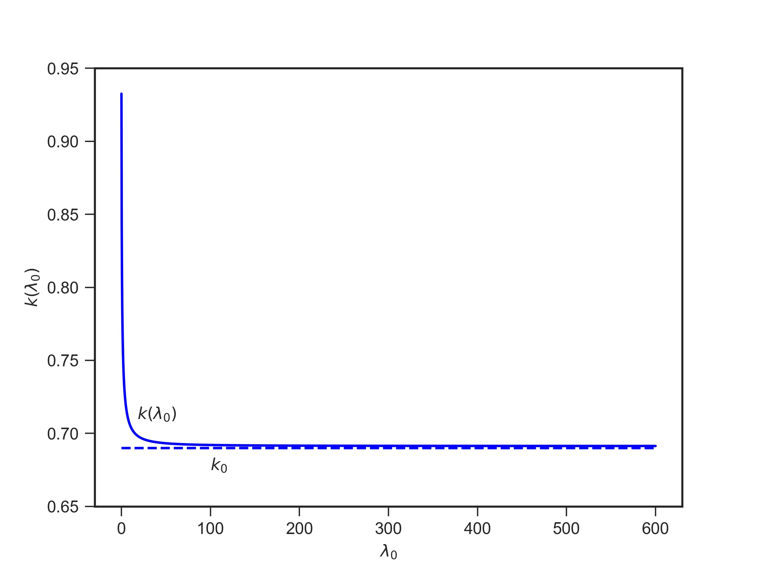
We first consider the limit of k=k⁡(λ0,λ1)k=k(\lambda_{0},\lambda_{1}) as λ0→∞\lambda_{0}\to\infty with λ1\lambda_{1} fixed. In this case, the mean time for αt\alpha_{t} spent at state 0 is given by (1/λ0)(1/\lambda_{0}) which goes to 0. In view of this, the limit of kk should correspond to the threshold of unconstrained pairs selling.

To validate this observation, we list all the terms in (21) that are λ0\lambda_{0} depended:

η=λ0λ1, 1−a0=ρ−μ1ρ−μ1+λ0, 1−a1=ρ−μ2ρ−μ2+λ0,γ2≈λ0σ,and​δ3≈−λ0σ.\eta=\frac{\lambda_{0}}{\lambda_{1}},\ 1-a_{0}=\frac{\rho-\mu_{1}}{\rho-\mu_{1}+\lambda_{0}},\ 1-a_{1}=\frac{\rho-\mu_{2}}{\rho-\mu_{2}+\lambda_{0}},\ \gamma_{2}\approx\frac{\sqrt{\lambda_{0}}}{\sqrt{\sigma}},\ \text{and}\ \delta_{3}\approx-\frac{\sqrt{\lambda_{0}}}{\sqrt{\sigma}}.

Therefore, we have

limλ0→∞k=limλ0→∞−2δ1λ03/2/(λ1σ)+lower order terms2​(1−δ1)​λ03/2/(λ1​σ)+lower order terms⋅βsβb=−δ11−δ1⋅βsβb=:k0.\lim_{\lambda_{0}\to\infty}k=\lim_{\lambda_{0}\to\infty}\frac{-2\delta_{1}\lambda_{0}^{3/2}/(\lambda_{1}\sqrt{\sigma})+\text{lower order terms}}{2(1-\delta_{1})\lambda_{0}^{3/2}/(\lambda_{1}\sqrt{\sigma})+\text{lower order terms}}\cdot\frac{\beta_{\rm s}}{\beta_{\rm b}}=\frac{-\delta_{1}}{1-\delta_{1}}\cdot\frac{\beta_{\rm s}}{\beta_{\rm b}}=:k_{0}.

To see the connection with the selling rule without constraints. We note that the associated HJB equation (unconstrained) has the form:

min⁡{ρ​w​(y)−ℒ​w​(y),w⁡(y)−βs+βb​y}=0.\min\Big\{\rho w(y)-{\mathcal{L}}w(y),\ w(y)-\beta_{\rm s}+\beta_{\rm b}y\Big\}=0.

Repeating our previous smooth-fit calculation yields exactly k=k0k=k_{0} obtained above.

Asymptotics of kk as λ1→∞\lambda_{1}\to\infty

Similarly, we can consider the limit λ1→∞\lambda_{1}\to\infty with fixed λ0\lambda_{0}. Note that δ3≈−λ1/σ\delta_{3}\approx-{\sqrt{\lambda_{1}}}/{\sqrt{\sigma}} and η=λ0/λ1\eta={\lambda_{0}}/{\lambda_{1}} are the only two terms depending on λ1\lambda_{1}. It follows that

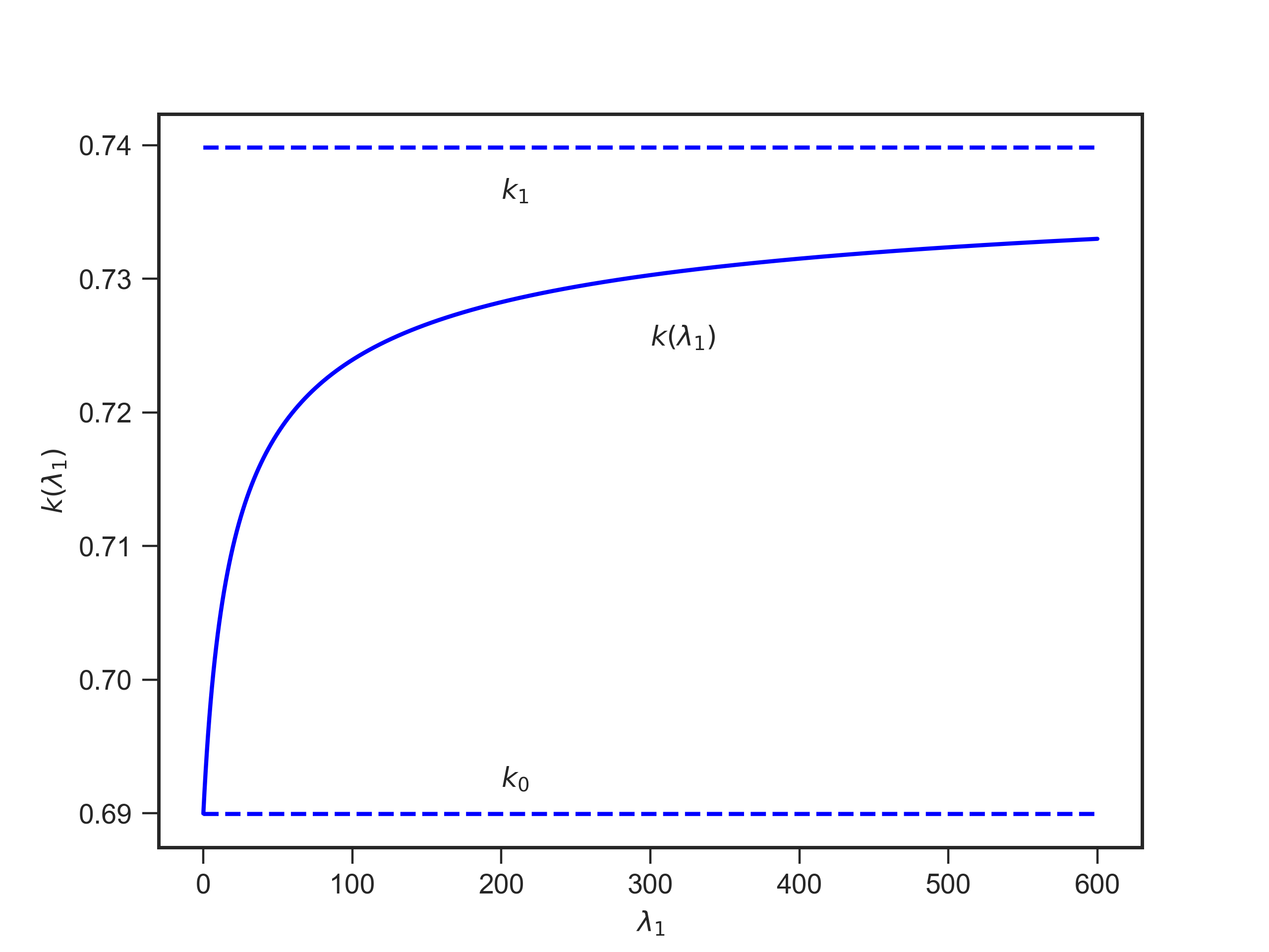
limλ1→∞k=δ1−γ2​(1−a0)δ1−[a1+γ2​(1−a1)]⋅βsβb=−δ1+γ2​(1−a0)1−δ1+(γ2−1)​(1−a1)⋅βsβb=:k1.\lim_{\lambda_{1}\to\infty}k=\frac{\delta_{1}-\gamma_{2}(1-a_{0})}{\delta_{1}-[a_{1}+\gamma_{2}(1-a_{1})]}\cdot\frac{\beta_{\rm s}}{\beta_{\rm b}}=\frac{-\delta_{1}+\gamma_{2}(1-a_{0})}{1-\delta_{1}+(\gamma_{2}-1)(1-a_{1})}\cdot\frac{\beta_{\rm s}}{\beta_{\rm b}}=:k_{1}.

It is not difficult to show k1>k0k_{1}>k_{0}. (Actually, it is equivalent to the inequality in (28) that is proved in the Appendix.) Intuitively, this makes sense because one has to make trading easier (with larger kk) when trading constraints are present.

6 Numerical Examples

In this section, we consider the trading pair of Target Corp. (TGT) and Walmart Stores Inc. (WMT). The model is calibrated by using the daily closing prices from 1985-1999. Let 𝐒1{\mathbf{S}}^{1}=WMT and 𝐒2{\mathbf{S}}^{2}=TGT. Using the traditional least squares method, we have μ1=0.2459\mu_{1}=0.2459, μ2=0.2059\mu_{2}=0.2059, σ11=0.2943\sigma_{11}=0.2943, σ12=0.0729\sigma_{12}=0.0729, σ21=0.0729\sigma_{21}=0.0729, and σ22=0.3112\sigma_{22}=0.3112. We take ρ=0.5\rho=0.5, λ0=λ1=10\lambda_{0}=\lambda_{1}=10, and K=0.001K=0.001. Using (21), we obtain k=0.7036k=0.7036. We plot the corresponding w0​(y)w_{0}(y) and w1​(y)w_{1}(y) in Figure 1 and vi(x1,x2)=x1wi(x2/x1),i=0,1v_{i}(x_{1},x_{2})=x_{1}w_{i}(x_{2}/x_{1}),i=0,1 in Figure 2.

Refer to caption
Refer to caption
Figure 1: Functions w0w_{0} and w1w_{1}
Refer to caption
Refer to caption
Figure 2: Functions v0v_{0} and v1v_{1}

Asymptotics of k⁡(λ0,λ1)k(\lambda_{0},\lambda_{1}).

Next, we examine the asymptotics of k=k⁡(λ0,λ1)k=k(\lambda_{0},\lambda_{1}) as one of λ0\lambda_{0} and λ1\lambda_{1} goes to ∞\infty with the other fixed (at 10). The corresponding graphs are plotted in Figure 3 along with y=k0y=k_{0} and y=k1y=k_{1}.

Refer to caption
Refer to caption
Figure 3: Asymptotics of k⁡(λ0,10)k(\lambda_{0},10) and k⁡(10,λ1)k(10,\lambda_{1})

In addition, we give the 2D graph of k⁡(λ0,λ1)k(\lambda_{0},\lambda_{1}) in Figure 4.

Refer to caption
Figure 4: Dependence of kk on λ0,λ1\lambda_{0},\lambda_{1}

Dependence of kk on various parameters.

In this section, we fix λ0=λ1=10\lambda_{0}=\lambda_{1}=10. We vary one parameter at a time and examine the dependence of kk on μi,σi​j,i,j=1,2,K,ρ\mu_{i},\sigma_{ij},i,j=1,2,K,\rho respectively.

First, we vary μi,i=1,2\mu_{i},i=1,2. Recall that we close the position by selling X1X^{1} and buying back X2X^{2} on [0,k][0,k] in the state α=1\alpha=1. A larger μi\mu_{i} implies greater growth potential in XiX^{i}. It can be seen in Table 1 that kk decrease in μ1\mu_{1} leading to fewer selling opportunities and kk increases in μ2\mu_{2} leading to more selling opportunities. It is because a larger μ2\mu_{2} and a smaller μ1\mu_{1} will encourage its early exit.

Table 1: kk with varying μ1,μ2\mu_{1},\mu_{2}
μ1\mu_{1} 0.1259 0.1659 0.2059 0.2459 0.2859
kk 0.7834 0.7481 0.7036 0.6481 0.5798
μ2\mu_{2} 0.1659 0.2059 0.2459 0.2859 0.3259
kk 0.6332 0.6688 0.7036 0.7367 0.7669

Next, we vary σ11\sigma_{11} and σ22\sigma_{22}. Larger volatility leads to a bigger room for the prices to move. This is associated with a smaller selling zone and therefore smaller kk.

Table 2: kk with varying σ11,σ22\sigma_{11},\sigma_{22}
σ11\sigma_{11} 0.2312 0.2712 0.3112 0.3512 0.3912
kk 0.7516 0.7286 0.7036 0.6777 0.6514
σ22\sigma_{22} 0.2143 0.2543 0.2943 0.3343 0.3743
kk 0.7469 0.7265 0.7036 0.6794 0.6543

Then, we vary σ12\sigma_{12} (=σ21)(=\sigma_{21}). Increasing these parameters makes the two stocks more related to each other which leads to a larger selling zone as shown in Table 3.

Table 3: kk with varying σ12=σ21\sigma_{12}=\sigma_{21}
σ12=σ21\sigma_{12}=\sigma_{21} -0.0129 0.0329 0.0729 0.1129 0.1529
kk 0.6060 0.6561 0.7036 0.75477 0.8094

Finally, we vary the discount rate ρ\rho and the transaction fee KK. Larger ρ\rho encourages to sell early which translates to a bigger selling zone as can be seen in Table 4. Additionally, larger KK sets up a higher barrier for selling which leads to a smaller selling zone.

Table 4: kk with varying ρ\rho and KK
ρ\rho 0.3 0.4 0.5 0.6 0.7
kk 0.5590 0.6541 0.7036 0.7358 0.7590
KK 0.0001 0.0005 0.001 0.002 0.003
kk 0.7049 0.7043 0.7036 0.7022 0.7008

7 Conclusion

The focus of this paper is on pairs selling with limited opportunities, and its main goal is to derive an optimal policy in closed form, which is desirable for practical applications.

It would be intriguing to extend the results of this study to models that incorporate more practical considerations, such as large block selling, where intensive trading may affect trading windows.

Overall, this paper contributes to the understanding of pairs selling and provides insights into developing optimal policies that can be applied in real-world scenarios. There is potential for future research to expand on these findings and explore more complex models that better capture real-world dynamics.

Appendix

In this appendix, we provide the proof of Lemma 3.1.

Proof of Lemma 3.1. We first work on C1C_{1} and C3C_{3}. In view of (22), C1>0C_{1}>0 and C3>0C_{3}>0 are equivalent to

−δ11−δ1⋅βsβb<k<−δ31−δ3⋅βsβb.\frac{-\delta_{1}}{1-\delta_{1}}\cdot\frac{\beta_{s}}{\beta_{b}}<k<\frac{-\delta_{3}}{1-\delta_{3}}\cdot\frac{\beta_{s}}{\beta_{b}}. (25)

To simplify notation, let b0=1−a0b_{0}=1-a_{0} and b1=1−a1b_{1}=1-a_{1}. Note that 0<b0<10<b_{0}<1 and 0<b1<10<b_{1}<1. Using this notation, we rewrite kk as

k=(1+η)​(−δ1)​(γ2−δ3)+b0​(δ1−δ3)​γ2(1+η)​(γ2−δ3)​(1−δ1)+b1​(γ2−1)​(δ1−δ3)⋅βsβb.k=\frac{(1+\eta)(-\delta_{1})(\gamma_{2}-\delta_{3})+b_{0}(\delta_{1}-\delta_{3})\gamma_{2}}{(1+\eta)(\gamma_{2}-\delta_{3})(1-\delta_{1})+b_{1}(\gamma_{2}-1)(\delta_{1}-\delta_{3})}\cdot\frac{\beta_{\rm s}}{\beta_{\rm b}}. (26)

The inequalities are equivalent to

−δ11−δ1<(1+η)​(−δ1)​(γ2−δ3)+b0​(δ1−δ3)​γ2(1+η)​(γ2−δ3)​(1−δ1)+b1​(γ2−1)​(δ1−δ3)<−δ31−δ3.\frac{-\delta_{1}}{1-\delta_{1}}<\frac{(1+\eta)(-\delta_{1})(\gamma_{2}-\delta_{3})+b_{0}(\delta_{1}-\delta_{3})\gamma_{2}}{(1+\eta)(\gamma_{2}-\delta_{3})(1-\delta_{1})+b_{1}(\gamma_{2}-1)(\delta_{1}-\delta_{3})}<\frac{-\delta_{3}}{1-\delta_{3}}. (27)

First inequality of (27).

The first inequality in (27) is equivalent to

b1​(γ2−1)​(δ1−δ3)​(−δ1)<b0​γ2​(δ1−δ3)​(1−δ1)⟺b1​(γ2−1)​(−δ1)<b0​γ2​(1−δ1).b_{1}(\gamma_{2}-1)(\delta_{1}-\delta_{3})(-\delta_{1})<b_{0}\gamma_{2}(\delta_{1}-\delta_{3})(1-\delta_{1})\ \Longleftrightarrow\ b_{1}(\gamma_{2}-1)(-\delta_{1})<b_{0}\gamma_{2}(1-\delta_{1}).

The last inequality is equivalent to

b1b0<γ2γ2−1⋅(1−1δ1)=(1+1γ2−1)​(1−1δ1).\frac{b_{1}}{b_{0}}<\frac{\gamma_{2}}{\gamma_{2}-1}\cdot(1-\frac{1}{\delta_{1}})=\left(1+\frac{1}{\gamma_{2}-1}\right)\left(1-\frac{1}{\delta_{1}}\right). (28)

Note that

b0=ρ−μ1ρ+λ0−μ1​ and ​b1=ρ−μ2ρ+λ0−μ2.b_{0}=\frac{\rho-\mu_{1}}{\rho+\lambda_{0}-\mu_{1}}\mbox{ and }b_{1}=\frac{\rho-\mu_{2}}{\rho+\lambda_{0}-\mu_{2}}.

We consider two cases: Case I (μ1≤μ2\mu_{1}\leq\mu_{2}) and Case II (μ1>μ2\mu_{1}>\mu_{2}).

Case I: If μ1≤μ2\mu_{1}\leq\mu_{2}, then

b1b0=1+λ0ρ−μ11+λ0ρ−μ2≤1;\frac{b_{1}}{b_{0}}=\frac{1+\frac{\lambda_{0}}{\rho-\mu_{1}}}{1+\frac{\lambda_{0}}{\rho-\mu_{2}}}\leq 1;

and the right hand side (28) is bigger than 11 since γ2>1\gamma_{2}>1 and δ1<0\delta_{1}<0. So the first inequality in (27) follows.

Case II: If μ1>μ2\mu_{1}>\mu_{2}, then

b1b0=1+λ0ρ−μ11+λ0ρ−μ2=(ρ+λ0−μ1)​(ρ−μ2)(ρ+λ0−μ2)​(ρ−μ1)>1.\frac{b_{1}}{b_{0}}=\frac{1+\frac{\lambda_{0}}{\rho-\mu_{1}}}{1+\frac{\lambda_{0}}{\rho-\mu_{2}}}=\frac{(\rho+\lambda_{0}-\mu_{1})(\rho-\mu_{2})}{(\rho+\lambda_{0}-\mu_{2})(\rho-\mu_{1})}>1.

The previous simple argument no longer works. We need to elaborate the value of (1+1γ2−1)​(1−1δ1)\left(1+\frac{1}{\gamma_{2}-1}\right)\left(1-\frac{1}{\delta_{1}}\right). To this end, note that

γ2γ2−1\displaystyle\frac{\gamma_{2}}{\gamma_{2}-1} =1+μ1−μ2σ+(1+μ1−μ2σ)2+4​(ρ+λ0−μ1)σ−1+μ1−μ2σ+(1+μ1−μ2σ)2+4​(ρ+λ0−μ1)σ\displaystyle=\frac{1+\frac{\mu_{1}-\mu_{2}}{\sigma}+\sqrt{\left(1+\frac{\mu_{1}-\mu_{2}}{\sigma}\right)^{2}+\frac{4(\rho+\lambda_{0}-\mu_{1})}{\sigma}}}{-1+\frac{\mu_{1}-\mu_{2}}{\sigma}+\sqrt{\left(1+\frac{\mu_{1}-\mu_{2}}{\sigma}\right)^{2}+\frac{4(\rho+\lambda_{0}-\mu_{1})}{\sigma}}}
=ρ+λ0+σ+σ​B1−μ1−μ22ρ+λ0−μ2,\displaystyle=\frac{\rho+\lambda_{0}+\frac{\sigma+\sigma\sqrt{B_{1}}-\mu_{1}-\mu_{2}}{2}}{\rho+\lambda_{0}-\mu_{2}},

where

B1=(1+μ1−μ2σ)2+4​(ρ+λ0−μ1)σ.B_{1}=\left(1+\frac{\mu_{1}-\mu_{2}}{\sigma}\right)^{2}+\frac{4(\rho+\lambda_{0}-\mu_{1})}{\sigma}.

Next we compute

δ1−1δ1\displaystyle\frac{\delta_{1}-1}{\delta_{1}} =−1+μ1−μ2σ−(1+μ1−μ2σ)2+4​(ρ−μ1)σ1+μ1−μ2σ−(1+μ1−μ2σ)2+4​(ρ−μ1)σ\displaystyle=\frac{-1+\frac{\mu_{1}-\mu_{2}}{\sigma}-\sqrt{\left(1+\frac{\mu_{1}-\mu_{2}}{\sigma}\right)^{2}+\frac{4(\rho-\mu_{1})}{\sigma}}}{1+\frac{\mu_{1}-\mu_{2}}{\sigma}-\sqrt{\left(1+\frac{\mu_{1}-\mu_{2}}{\sigma}\right)^{2}+\frac{4(\rho-\mu_{1})}{\sigma}}}
=1−μ1−μ2σ+(1+μ1−μ2σ)2+4​(ρ−μ1)σ−1−μ1−μ2σ+(1+μ1−μ2σ)2+4​(ρ−μ1)σ\displaystyle=\frac{1-\frac{\mu_{1}-\mu_{2}}{\sigma}+\sqrt{\left(1+\frac{\mu_{1}-\mu_{2}}{\sigma}\right)^{2}+\frac{4(\rho-\mu_{1})}{\sigma}}}{-1-\frac{\mu_{1}-\mu_{2}}{\sigma}+\sqrt{\left(1+\frac{\mu_{1}-\mu_{2}}{\sigma}\right)^{2}+\frac{4(\rho-\mu_{1})}{\sigma}}}
=ρ+σ+σ​B2−μ1−μ22ρ−μ1,\displaystyle=\frac{\rho+\frac{\sigma+\sigma\sqrt{B_{2}}-\mu_{1}-\mu_{2}}{2}}{\rho-\mu_{1}},

where

B2=(1+μ1−μ2σ)2+4​(ρ−μ1)σ.B_{2}=\left(1+\frac{\mu_{1}-\mu_{2}}{\sigma}\right)^{2}+\frac{4(\rho-\mu_{1})}{\sigma}.

Since μ1>μ2\mu_{1}>\mu_{2}, we have

B1>1+μ1−μ2σandB2>1+μ1−μ2σ.\sqrt{B_{1}}>1+\frac{\mu_{1}-\mu_{2}}{\sigma}\quad\text{and}\quad\sqrt{B_{2}}>1+\frac{\mu_{1}-\mu_{2}}{\sigma}.

This implies

σ+σ​B1−μ1−μ22>σ−μ2,σ+σ​B2−μ1−μ22>σ−μ2,\frac{\sigma+\sigma\sqrt{B_{1}}-\mu_{1}-\mu_{2}}{2}>\sigma-\mu_{2},\quad\frac{\sigma+\sigma\sqrt{B_{2}}-\mu_{1}-\mu_{2}}{2}>\sigma-\mu_{2},

and

(1+1γ2−1)​(1−1δ1)\displaystyle\left(1+\frac{1}{\gamma_{2}-1}\right)\left(1-\frac{1}{\delta_{1}}\right) >ρ+λ0+σ−μ2ρ+λ0−μ2⋅ρ+σ−μ2ρ−μ1\displaystyle>\frac{\rho+\lambda_{0}+\sigma-\mu_{2}}{\rho+\lambda_{0}-\mu_{2}}\cdot\frac{\rho+\sigma-\mu_{2}}{\rho-\mu_{1}}
>(ρ+λ0−μ1)​(ρ−μ2)(ρ+λ0−μ2)​(ρ−μ1).\displaystyle>\frac{(\rho+\lambda_{0}-\mu_{1})(\rho-\mu_{2})}{(\rho+\lambda_{0}-\mu_{2})(\rho-\mu_{1})}.

This is exactly what we need to show. Here we have used

ρ+λ0+σ−μ2>ρ+λ0−μ1​and​ρ+σ−μ2>ρ−μ2,\rho+\lambda_{0}+\sigma-\mu_{2}>\rho+\lambda_{0}-\mu_{1}\ \text{and}\ \rho+\sigma-\mu_{2}>\rho-\mu_{2},

since μ1>μ2\mu_{1}>\mu_{2} and σ>0\sigma>0.

Second inequality of (27).

The second inequality in (27) is equivalent to

(1+η)​(−δ1)​(γ2−δ3)​(1−δ3)+b0​γ2​(δ1−δ3)​(1−δ3)\displaystyle(1+\eta)(-\delta_{1})(\gamma_{2}-\delta_{3})(1-\delta_{3})+b_{0}\gamma_{2}(\delta_{1}-\delta_{3})(1-\delta_{3})
<\displaystyle< (1+η)​(γ2−δ3)​(1−δ1)​(−δ3)+b1​(γ2−1)​(δ1−δ3)​(−δ3).\displaystyle(1+\eta)(\gamma_{2}-\delta_{3})(1-\delta_{1})(-\delta_{3})+b_{1}(\gamma_{2}-1)(\delta_{1}-\delta_{3})(-\delta_{3}).

This is equivalent to

b0​γ2​(1−δ3)<(1+η)​(γ2−δ3)+b1​(γ2−1)​(−δ3).b_{0}\gamma_{2}(1-\delta_{3})<(1+\eta)(\gamma_{2}-\delta_{3})+b_{1}(\gamma_{2}-1)(-\delta_{3}).

We will let a=−δ3>0a=-\delta_{3}>0 and γ2=1+γ\gamma_{2}=1+\gamma. Then, the above inequality is reduced to

b0​(1+γ)​(1+a)<(1+η)​(1+γ+a)+b1​γ​a.b_{0}(1+\gamma)(1+a)<(1+\eta)(1+\gamma+a)+b_{1}\gamma a.

Since 1+γ+a=(1+a)​(1+γ)−a​γ1+\gamma+a=(1+a)(1+\gamma)-a\gamma, the above inequality is equivalent to

(1+η−b1)aγ<(1+η−b0)(1+a)(1+γ)⟺1+η−b11+η−b0<(1+a)​(1+γ)a​γ.(1+\eta-b_{1})a\gamma<(1+\eta-b_{0})(1+a)(1+\gamma)\quad\Longleftrightarrow\quad\frac{1+\eta-b_{1}}{1+\eta-b_{0}}<\frac{(1+a)(1+\gamma)}{a\gamma}.

Then, we have

1+η−b11+η−b0\displaystyle\frac{1+\eta-b_{1}}{1+\eta-b_{0}} =1+λ0λ1−ρ−μ2ρ+λ0−μ21+λ0λ1−ρ−μ1ρ+λ0−μ1=λ0λ1+λ0ρ+λ0−μ2λ0λ1+λ0ρ+λ0−μ1\displaystyle=\frac{1+\frac{\lambda_{0}}{\lambda_{1}}-\frac{\rho-\mu_{2}}{\rho+\lambda_{0}-\mu_{2}}}{1+\frac{\lambda_{0}}{\lambda_{1}}-\frac{\rho-\mu_{1}}{\rho+\lambda_{0}-\mu_{1}}}=\frac{\frac{\lambda_{0}}{\lambda_{1}}+\frac{\lambda_{0}}{\rho+\lambda_{0}-\mu_{2}}}{\frac{\lambda_{0}}{\lambda_{1}}+\frac{\lambda_{0}}{\rho+\lambda_{0}-\mu_{1}}}
=1+λ1ρ+λ0−μ21+λ1ρ+λ0−μ1=(ρ+λ0+λ1−μ2)​(ρ+λ0−μ1)(ρ+λ0+λ1−μ1)​(ρ+λ0−μ2),\displaystyle=\frac{1+\frac{\lambda_{1}}{\rho+\lambda_{0}-\mu_{2}}}{1+\frac{\lambda_{1}}{\rho+\lambda_{0}-\mu_{1}}}=\frac{(\rho+\lambda_{0}+\lambda_{1}-\mu_{2})(\rho+\lambda_{0}-\mu_{1})}{(\rho+\lambda_{0}+\lambda_{1}-\mu_{1})(\rho+\lambda_{0}-\mu_{2})},

and

(1+a)​(1+γ)a​γ\displaystyle\frac{(1+a)(1+\gamma)}{a\gamma} =(1+1a)​(1+1γ).\displaystyle=\left(1+\frac{1}{a}\right)\left(1+\frac{1}{\gamma}\right).

Recall that

a=−δ3\displaystyle a=-\delta_{3} =12​[(1+μ1−μ2σ)2+4​(ρ+λ0+λ1−μ1)σ−(1+μ1−μ2σ)],\displaystyle=\frac{1}{2}\left[\sqrt{\left(1+\frac{\mu_{1}-\mu_{2}}{\sigma}\right)^{2}+\frac{4(\rho+\lambda_{0}+\lambda_{1}-\mu_{1})}{\sigma}}-\left(1+\frac{\mu_{1}-\mu_{2}}{\sigma}\right)\right],
a+1\displaystyle a+1 =12​[(1+μ1−μ2σ)2+4​(ρ+λ0+λ1−μ1)σ+(1−μ1−μ2σ)].\displaystyle=\frac{1}{2}\left[\sqrt{\left(1+\frac{\mu_{1}-\mu_{2}}{\sigma}\right)^{2}+\frac{4(\rho+\lambda_{0}+\lambda_{1}-\mu_{1})}{\sigma}}+\left(1-\frac{\mu_{1}-\mu_{2}}{\sigma}\right)\right].

Simple calculation yields

1+aa\displaystyle\frac{1+a}{a} =(1+μ1−μ2σ)2+4​(ρ+λ0+λ1−μ1)σ+(1−μ1−μ2σ)(1+μ1−μ2σ)2+4​(ρ+λ0+λ1−μ1)σ−(1+μ1−μ2σ)\displaystyle=\frac{\sqrt{\left(1+\frac{\mu_{1}-\mu_{2}}{\sigma}\right)^{2}+\frac{4(\rho+\lambda_{0}+\lambda_{1}-\mu_{1})}{\sigma}}+\left(1-\frac{\mu_{1}-\mu_{2}}{\sigma}\right)}{\sqrt{\left(1+\frac{\mu_{1}-\mu_{2}}{\sigma}\right)^{2}+\frac{4(\rho+\lambda_{0}+\lambda_{1}-\mu_{1})}{\sigma}}-\left(1+\frac{\mu_{1}-\mu_{2}}{\sigma}\right)}
=[(1+μ1−μ2σ)2+4​(ρ+λ0+λ1−μ1)σ+1]2−(μ1−μ2σ)24​(ρ+λ0+λ1−μ1)σ\displaystyle=\frac{\left[\sqrt{\left(1+\frac{\mu_{1}-\mu_{2}}{\sigma}\right)^{2}+\frac{4(\rho+\lambda_{0}+\lambda_{1}-\mu_{1})}{\sigma}}+1\right]^{2}-\left(\frac{\mu_{1}-\mu_{2}}{\sigma}\right)^{2}}{\frac{4(\rho+\lambda_{0}+\lambda_{1}-\mu_{1})}{\sigma}}
=2+4​(ρ+λ0+λ1−μ1)+2​μ1−2​μ2σ+2​B34​(ρ+λ0+λ1−μ1)σ\displaystyle=\frac{2+\frac{4(\rho+\lambda_{0}+\lambda_{1}-\mu_{1})+2\mu_{1}-2\mu_{2}}{\sigma}+2\sqrt{B_{3}}}{\frac{4(\rho+\lambda_{0}+\lambda_{1}-\mu_{1})}{\sigma}}
=ρ+λ0+λ1−μ1+μ22+1+B32​σρ+λ0+λ1−μ1,\displaystyle=\frac{\rho+\lambda_{0}+\lambda_{1}-\frac{\mu_{1}+\mu_{2}}{2}+\frac{1+\sqrt{B_{3}}}{2}\sigma}{\rho+\lambda_{0}+\lambda_{1}-\mu_{1}},

where

B3=(1+μ1−μ2σ)2+4​(ρ+λ0+λ1−μ1)σ.B_{3}=\left(1+\frac{\mu_{1}-\mu_{2}}{\sigma}\right)^{2}+\frac{4(\rho+\lambda_{0}+\lambda_{1}-\mu_{1})}{\sigma}.

Recall B1=(1+μ1−μ2σ)2+4​(ρ+λ0−μ1)σB_{1}=\left(1+\frac{\mu_{1}-\mu_{2}}{\sigma}\right)^{2}+\frac{4(\rho+\lambda_{0}-\mu_{1})}{\sigma}. We have

γ+1γ\displaystyle\frac{\gamma+1}{\gamma} =μ1−μ2σ+1+(μ1−μ2σ+1)2+4​(ρ+λ0−μ1)σμ1−μ2σ−1+(μ1−μ2σ+1)2+4​(ρ+λ0−μ1)σ\displaystyle=\frac{\frac{\mu_{1}-\mu_{2}}{\sigma}+1+\sqrt{\left(\frac{\mu_{1}-\mu_{2}}{\sigma}+1\right)^{2}+\frac{4(\rho+\lambda_{0}-\mu_{1})}{\sigma}}}{\frac{\mu_{1}-\mu_{2}}{\sigma}-1+\sqrt{\left(\frac{\mu_{1}-\mu_{2}}{\sigma}+1\right)^{2}+\frac{4(\rho+\lambda_{0}-\mu_{1})}{\sigma}}}
=ρ+λ0−μ1+μ22+1+B12​σρ+λ0−μ2.\displaystyle=\frac{\rho+\lambda_{0}-\frac{\mu_{1}+\mu_{2}}{2}+\frac{1+\sqrt{B_{1}}}{2}\sigma}{\rho+\lambda_{0}-\mu_{2}}.

Note that

B3>|1+μ1−μ2σ|andB1>|1+μ1−μ2σ|.\sqrt{B_{3}}>\left|1+\frac{\mu_{1}-\mu_{2}}{\sigma}\right|\quad\text{and}\quad\sqrt{B_{1}}>\left|1+\frac{\mu_{1}-\mu_{2}}{\sigma}\right|.

This implies

(1+B3)​σ2−μ1+μ22\displaystyle\frac{(1+\sqrt{B_{3}})\sigma}{2}-\frac{\mu_{1}+\mu_{2}}{2} >σ+|σ+μ1−μ2|−μ1−μ22\displaystyle>\frac{\sigma+|\sigma+\mu_{1}-\mu_{2}|-\mu_{1}-\mu_{2}}{2}
={σ−μ2σ+μ1>μ2,−μ1σ+μ1≤μ2.\displaystyle=\begin{cases}\sigma-\mu_{2}&\sigma+\mu_{1}>\mu_{2},\\ -\mu_{1}&\sigma+\mu_{1}\leq\mu_{2}.\end{cases}

and similarly

(1+B1)​σ2−μ1+μ22>{σ−μ2σ+μ1>μ2,−μ1σ+μ1≤μ2.\frac{(1+\sqrt{B_{1}})\sigma}{2}-\frac{\mu_{1}+\mu_{2}}{2}>\begin{cases}\sigma-\mu_{2}&\sigma+\mu_{1}>\mu_{2},\\ -\mu_{1}&\sigma+\mu_{1}\leq\mu_{2}.\end{cases}

This implies that if σ+μ1>μ2\sigma+\mu_{1}>\mu_{2} we have

(1+a)​(1+γ)a​γ\displaystyle\frac{(1+a)(1+\gamma)}{a\gamma} >ρ+λ0+λ1−μ2+σρ+λ0+λ1−μ1⋅ρ+λ0−μ2+σρ+λ0−μ2\displaystyle>\frac{\rho+\lambda_{0}+\lambda_{1}-\mu_{2}+\sigma}{\rho+\lambda_{0}+\lambda_{1}-\mu_{1}}\cdot\frac{\rho+\lambda_{0}-\mu_{2}+\sigma}{\rho+\lambda_{0}-\mu_{2}}
>(ρ+λ0+λ1−μ2)​(ρ+λ0−μ1)(ρ+λ0+λ1−μ1)​((ρ+λ0−μ2)CLOSE\displaystyle>\frac{(\rho+\lambda_{0}+\lambda_{1}-\mu_{2})(\rho+\lambda_{0}-\mu_{1})}{(\rho+\lambda_{0}+\lambda_{1}-\mu_{1})((\rho+\lambda_{0}-\mu_{2})}
=1+η−b11+η−b0.\displaystyle=\frac{1+\eta-b_{1}}{1+\eta-b_{0}}.

Here we have used σ+μ1−μ2>0\sigma+\mu_{1}-\mu_{2}>0 hence σ−μ2>−μ1\sigma-\mu_{2}>-\mu_{1} and

ρ+λ0−μ2+σ>ρ+λ0−μ1.\rho+\lambda_{0}-\mu_{2}+\sigma>\rho+\lambda_{0}-\mu_{1}.

If σ+μ1≤μ2\sigma+\mu_{1}\leq\mu_{2}, then μ1<σ+μ1≤μ2\mu_{1}<\sigma+\mu_{1}\leq\mu_{2} and

ρ+λ0+λ1−μ1>ρ+λ0+λ1−μ2\rho+\lambda_{0}+\lambda_{1}-\mu_{1}>\rho+\lambda_{0}+\lambda_{1}-\mu_{2}

and

(1+a)​(1+γ)a​γ\displaystyle\frac{(1+a)(1+\gamma)}{a\gamma} >ρ+λ0+λ1−μ1ρ+λ0+λ1−μ1⋅ρ+λ0−μ1ρ+λ0−μ2\displaystyle>\frac{\rho+\lambda_{0}+\lambda_{1}-\mu_{1}}{\rho+\lambda_{0}+\lambda_{1}-\mu_{1}}\cdot\frac{\rho+\lambda_{0}-\mu_{1}}{\rho+\lambda_{0}-\mu_{2}}
>(ρ+λ0+λ1−μ2)​(ρ+λ0−μ1)(ρ+λ0+λ1−μ1)​((ρ+λ0−μ2)CLOSE\displaystyle>\frac{(\rho+\lambda_{0}+\lambda_{1}-\mu_{2})(\rho+\lambda_{0}-\mu_{1})}{(\rho+\lambda_{0}+\lambda_{1}-\mu_{1})((\rho+\lambda_{0}-\mu_{2})}
=1+η−b11+η−b0.\displaystyle=\frac{1+\eta-b_{1}}{1+\eta-b_{0}}.

This exactly what we need to prove for the second inequality in (27).

Proof of C2>0C_{2}>0

Recall C2C_{2} given in (24). In that formula, the denominator is positive since δ3<δ1<0\delta_{3}<\delta_{1}<0, γ2>1\gamma_{2}>1, and 0<a0,a1<10<a_{0},\ a_{1}<1. C2C_{2} is positive if

(1−a0)​(η+a1)​(1−δ1)​(−δ3)>(1−a1)​(η+a0)​(1−δ3)​(−δ1).(1-a_{0})(\eta+a_{1})(1-\delta_{1})(-\delta_{3})>(1-a_{1})(\eta+a_{0})(1-\delta_{3})(-\delta_{1}).

Since δ1<0\delta_{1}<0 and δ3<0\delta_{3}<0, this is equivalent to

η+a11−a1⋅−δ11−δ1>η+a01−a0⋅1−δ3−δ3.\frac{\eta+a_{1}}{1-a_{1}}\cdot\frac{-\delta_{1}}{1-\delta_{1}}>\frac{\eta+a_{0}}{1-a_{0}}\cdot\frac{1-\delta_{3}}{-\delta_{3}}. (29)

We need to compute both sides and compare them. Note that

η+a11−a1\displaystyle\frac{\eta+a_{1}}{1-a_{1}} =λ0λ1+λ0ρ+λ0−μ2ρ−μ2ρ+λ0−μ2=λ0λ1⋅ρ+λ0+λ1−μ2ρ−μ2,\displaystyle=\frac{\frac{\lambda_{0}}{\lambda_{1}}+\frac{\lambda_{0}}{\rho+\lambda_{0}-\mu_{2}}}{\frac{\rho-\mu_{2}}{\rho+\lambda_{0}-\mu_{2}}}=\frac{\lambda_{0}}{\lambda_{1}}\cdot\frac{\rho+\lambda_{0}+\lambda_{1}-\mu_{2}}{\rho-\mu_{2}},
η+a01−a0\displaystyle\frac{\eta+a_{0}}{1-a_{0}} =λ0λ1+λ0ρ+λ0−μ1ρ−μ1ρ+λ0−μ1=λ0λ1⋅ρ+λ0+λ1−μ1ρ−μ1.\displaystyle=\frac{\frac{\lambda_{0}}{\lambda_{1}}+\frac{\lambda_{0}}{\rho+\lambda_{0}-\mu_{1}}}{\frac{\rho-\mu_{1}}{\rho+\lambda_{0}-\mu_{1}}}=\frac{\lambda_{0}}{\lambda_{1}}\cdot\frac{\rho+\lambda_{0}+\lambda_{1}-\mu_{1}}{\rho-\mu_{1}}.

Then (29) is reduced to

ρ+λ0+λ1−μ2ρ−μ2⋅1−δ1−δ1>ρ+λ0+λ1−μ1ρ−μ1⋅1−δ3−δ3.\frac{\rho+\lambda_{0}+\lambda_{1}-\mu_{2}}{\rho-\mu_{2}}\cdot\frac{1-\delta_{1}}{-\delta_{1}}>\frac{\rho+\lambda_{0}+\lambda_{1}-\mu_{1}}{\rho-\mu_{1}}\cdot\frac{1-\delta_{3}}{-\delta_{3}}. (30)

Recall that

1−δ1−δ1=ρ−μ1+μ22+1+B22​σρ−μ1, and ​1−δ3−δ3=ρ+λ0+λ1−μ1+μ22+1+B32​σρ+λ0+λ1−μ1.\frac{1-\delta_{1}}{-\delta_{1}}=\frac{\rho-\frac{\mu_{1}+\mu_{2}}{2}+\frac{1+\sqrt{B_{2}}}{2}\sigma}{\rho-\mu_{1}},\mbox{ and }\frac{1-\delta_{3}}{-\delta_{3}}=\frac{\rho+\lambda_{0}+\lambda_{1}-\frac{\mu_{1}+\mu_{2}}{2}+\frac{1+\sqrt{B_{3}}}{2}\sigma}{\rho+\lambda_{0}+\lambda_{1}-\mu_{1}}.

Then (30) is reduced to

ρ+λ0+λ1−μ2ρ−μ2​(ρ−μ1+μ22+1+B22​σ)>ρ+λ0+λ1−μ1+μ22+1+B32​σ.\frac{\rho+\lambda_{0}+\lambda_{1}-\mu_{2}}{\rho-\mu_{2}}\left(\rho-\frac{\mu_{1}+\mu_{2}}{2}+\frac{1+\sqrt{B_{2}}}{2}\sigma\right)>\rho+\lambda_{0}+\lambda_{1}-\frac{\mu_{1}+\mu_{2}}{2}+\frac{1+\sqrt{B_{3}}}{2}\sigma.

This is equivalent to

(ρ+λ0+λ1−μ2)​(ρ−μ1+μ2−σ2)−(ρ+λ0+λ1−μ1+μ2−σ2)​(ρ−μ2)\displaystyle(\rho+\lambda_{0}+\lambda_{1}-\mu_{2})\left(\rho-\frac{\mu_{1}+\mu_{2}-\sigma}{2}\right)-\left(\rho+\lambda_{0}+\lambda_{1}-\frac{\mu_{1}+\mu_{2}-\sigma}{2}\right)(\rho-\mu_{2})
>\displaystyle> (ρ−μ2)​B32​σ−(ρ+λ0+λ1−μ2)​B22​σ\displaystyle(\rho-\mu_{2})\frac{\sqrt{B_{3}}}{2}\sigma-(\rho+\lambda_{0}+\lambda_{1}-\mu_{2})\frac{\sqrt{B_{2}}}{2}\sigma
=\displaystyle= σ2​(ρ−μ2)​(B3−B2)−(λ0+λ1)​B22​σ.\displaystyle\frac{\sigma}{2}(\rho-\mu_{2})(\sqrt{B_{3}}-\sqrt{B_{2}})-(\lambda_{0}+\lambda_{1})\frac{\sqrt{B_{2}}}{2}\sigma.

We can simplify the above inequality and it is equivalent to

(λ0+λ1)​(1+μ2−μ1σ+B2)>(ρ−μ2)​(B3−B2).(\lambda_{0}+\lambda_{1})(1+\frac{\mu_{2}-\mu_{1}}{\sigma}+\sqrt{B_{2}})>(\rho-\mu_{2})(\sqrt{B_{3}}-\sqrt{B_{2}}). (31)

Note that

B3−B2=B3−B2B3+B2=4​(λ0+λ1)σ⋅1B3+B2.\sqrt{B_{3}}-\sqrt{B_{2}}=\frac{B_{3}-B_{2}}{\sqrt{B_{3}}+\sqrt{B_{2}}}=\frac{4(\lambda_{0}+\lambda_{1})}{\sigma}\cdot\frac{1}{\sqrt{B_{3}}+\sqrt{B_{2}}}.

We can reduce (31) to

(1+μ2−μ1σ+B2)​(B3+B2)>4​(ρ−μ2)σ.\left(1+\frac{\mu_{2}-\mu_{1}}{\sigma}+\sqrt{B_{2}}\right)(\sqrt{B_{3}}+\sqrt{B_{2}})>\frac{4(\rho-\mu_{2})}{\sigma}.

This is equivalent to

(1+μ2−μ1σ+B2)​B3+(1+μ2−μ1σ)​B2>4​(ρ−μ2)σ−B2.\left(1+\frac{\mu_{2}-\mu_{1}}{\sigma}+\sqrt{B_{2}}\right)\sqrt{B_{3}}+\left(1+\frac{\mu_{2}-\mu_{1}}{\sigma}\right)\sqrt{B_{2}}>\frac{4(\rho-\mu_{2})}{\sigma}-B_{2}.

Then we note that

4​(ρ−μ2)σ−B2=4​(ρ−μ2)σ−(1+μ1−μ2σ)2−4​(ρ−μ1)σ\displaystyle\frac{4(\rho-\mu_{2})}{\sigma}-B_{2}=\frac{4(\rho-\mu_{2})}{\sigma}-\left(1+\frac{\mu_{1}-\mu_{2}}{\sigma}\right)^{2}-\frac{4(\rho-\mu_{1})}{\sigma}
=\displaystyle= 4​(μ1−μ2)σ−(1+μ1−μ2σ)2=−(1−μ1−μ2σ)2=−(1+μ2−μ1σ)2.\displaystyle\frac{4(\mu_{1}-\mu_{2})}{\sigma}-\left(1+\frac{\mu_{1}-\mu_{2}}{\sigma}\right)^{2}=-\left(1-\frac{\mu_{1}-\mu_{2}}{\sigma}\right)^{2}=-\left(1+\frac{\mu_{2}-\mu_{1}}{\sigma}\right)^{2}.

The inequality is equivalent to

(1+μ2−μ1σ+B2)​B3+(1+μ2−μ1σ)​B2>−(1+μ2−μ1σ)2.\left(1+\frac{\mu_{2}-\mu_{1}}{\sigma}+\sqrt{B_{2}}\right)\sqrt{B_{3}}+\left(1+\frac{\mu_{2}-\mu_{1}}{\sigma}\right)\sqrt{B_{2}}>-\left(1+\frac{\mu_{2}-\mu_{1}}{\sigma}\right)^{2}.

Moving the term −(1+μ2−μ1σ)2-\left(1+\frac{\mu_{2}-\mu_{1}}{\sigma}\right)^{2} to the left-hand side and we obtain

(1+μ2−μ1σ+B2)​(1+μ2−μ1σ+B3)>0.\left(1+\frac{\mu_{2}-\mu_{1}}{\sigma}+\sqrt{B_{2}}\right)\left(1+\frac{\mu_{2}-\mu_{1}}{\sigma}+\sqrt{B_{3}}\right)>0. (32)

Then we apply

B2>|1+μ1−μ2σ|andB3>|1+μ1−μ2σ|\sqrt{B_{2}}>|1+\frac{\mu_{1}-\mu_{2}}{\sigma}|\quad\text{and}\quad\sqrt{B_{3}}>|1+\frac{\mu_{1}-\mu_{2}}{\sigma}|

to obtain

1+μ2−μ1σ+B2>{2if σ>μ2−μ1,2​(μ2−μ1)σ≥2if σ≤μ2−μ1.1+\frac{\mu_{2}-\mu_{1}}{\sigma}+\sqrt{B_{2}}>\begin{cases}2&\text{if $\sigma>\mu_{2}-\mu_{1}$},\\ \frac{2(\mu_{2}-\mu_{1})}{\sigma}\geq 2&\text{if $\sigma\leq\mu_{2}-\mu_{1}$}.\end{cases}

Similarly, 1+μ2−μ1σ+B3>21+\frac{\mu_{2}-\mu_{1}}{\sigma}+\sqrt{B_{3}}>2. So (32) follows. Therefore, C2>0C_{2}>0. □\Box

Acknowledgments

This work is supported jointly by the Australian Research Council Discovery Project DP200101550, the Natural Science Foundation of China 11831010 and 61961160732, the Natural Science Foundation of Shandong Province ZR2019ZD42 and the Taishan Scholars Climbing Program of Shandong TSPD20210302.

References

  • [1] M. Dai, Q. Zhang, and Q. Zhu, Trend following trading under a regime switching model, SIAM J. Financial Mathematics 1 (2010), 780-810.
  • [2] A. Deshpande and B.R. Barmish, A general framework for pairs trading with a control-theoretic point of view, Proceedings of the IEEE Conference on Control Applications (CCA) September 19-22, 2016. Buenos Aires, Argentina.
  • [3] P. Dupuis and H. Wang, Optimal stopping with random intervention times, Adv. Appl. Probab. 34 (2002), pp. 141-157.
  • [4] R.J. Elliott, J. Van Der Hoek, and W.P. Malcolm, Pairs trading, Quantitative Finance 5 (2005), 271–276.
  • [5] E. Gatev, W.N. Goetzmann, and K.G. Rouwenhorst, Pairs trading: Performance of a relative-value arbitrage rule, Review of Financial Studies 19 (2006), 797-827.
  • [6] X. Guo and Q. Zhang, Optimal selling rules in a regime switching model, IEEE Transactions on Automatic Control 50 (2005), 1450-1455.
  • [7] Y. Hu and B. Øksendal, Optimal time to invest when the price processes are geometric Brownian motions, Finance and Stochastics 2 (1998), 295-310.
  • [8] S. Iwarere and B.R. Barmish, A confidence interval triggering method for stock trading via feedback control, Proc. American Control Conference 2010, Baltimore, MD.
  • [9] R. McDonald and D. Siegel, The value of waiting to invest, Quarterly J. Economics 101 (1986), 707-727.
  • [10] J.L. Menaldi and M. Robin, On some optimal stopping problems with constraint, SIAM J. Control Optim. 54, pp. 2650-2671, (2016).
  • [11] A. Merhi and M. Zervos, A model for reversible investment capacity expansion, SIAM J. Control. Optim. 46 (2007), 839-876.
  • [12] B. Ø{\O}ksendal, Stochastic Differential Equations, 6th Ed., Springer-Verlag, New York. 2003.
  • [13] Q.S. Song and Q. Zhang, An optimal pairs-trading rule, Automatica 49 (2013), 3007-3014.
  • [14] J. Tie, H. Zhang, and Q. Zhang, An Optimal strategy for pairs-trading under geometric Brownian motions, J. Optimization Theory Applications 179 (2018), 654-675.
  • [15] M. Whistler, Trading Pairs: Capturing Profits and Hedging Risk with Statistical Arbitrage Strategies, John Wiley and Sons, 2004.
  • [16] Q. Zhang, Stock trading: An optimal selling rule, SIAM J. Contr. Optim. 40 (2001), 64-87.
  • [17] H. Zhang and Q. Zhang, Trading a mean-reverting asset: Buy low and sell high, Automatica 44 (2008), 1511-1518.