Task-driven Semantic-aware Green Cooperative Transmission Strategy for Vehicular Networks

Based on our previous review works [6, 7], the existing research on SemCom can be broadly classified into four categories depending on the SE method. The first and most studied category is deep-learning (DL)-based end-to-end SemCom. The employed semantic encoder and decoder are two separate learnable neural networks, and linked through a layer for modeling random channels [17]. They are trained jointly, based on a complete data set shared by both senders and receivers. Thanks to the advancement of DL models, e.g., Transformer, the high efficient SE for text, image, and audio, achieves significantly performance gains especially at low signal-to-noise ratio (SNR) region [8, 18, 10]. Nevertheless, the back-propagation in DL paradigm requires the loss function to be differentiable, which hinders the sophisticated non-differentiable semantic metrics from being applied to guide the training. To solve this issue, deep reinforcement learning paradigm is adopted to perform SE [19]. However, the above two categories of SemCom are available only for the simplest point-to-point communication model, which cannot be directly applied to complex real-world scenarios. Moreover, the black box nature also restricts their social acceptance [6].

Meanwhile, with the development of the explainability of AI technologies, some researchers propose the knowledge base (KB)-assisted SemCom. Herein, the KB is a special database for semantic knowledge management, which consists of semantic elements embedded in the source data, the involving communication tasks, and the possible ways of reasoning by communication participants [7]. Up to now, there are two available kinds of general KB models. One is based on a hierarchical structure [20], and the other is based on graph structure [21, 7]. Moreover, there have been several technical research [22, 23] on SemCom for text transmission based on the available the interconversion technologies for text and graph. However, in the above works, the resource allocation algorithm is still following the philosophy of traditional content-blind resource allocation paradigm, i.e., allocating radio resources to per user according to their required data volume. In this sense, a semantic-aware transmission has not been achieved in a real sense.

In addition to the above three categories of SemCom, there is also a semantic-native SemCom paradigm, wherein the semantic information can be learned from iterative communications between intelligent agents [24]. However, this study is still stuck in the theoretical analysis based on a simple ideal model. It remains a huge challenge to put it into practice. In this sense, we focus on the KB-assisted SemCom in our work.

The core concept of SCFS is to utilize the mobility of relays to physically propagate information messages [15], which is first proposed in [25]. Specifically, in SCFS, a relay vehicle, which will pass the target vehicle within their uncovered area, pre-stores partial data requested by the target vehicle in advance over an available V2I link. It then carries and forwards data to the target vehicle until they encounter each other.

Initially, in [26, 27], the authors investigate the optimization of the target vehicle speed control with the objective of minimization of the outage time. However, it deviates from the design philosophy of user experience-oriented communication nowadays, and it is unrealistic to control the vehicle’s speed without consideration of the actual traffic conditions and the driver’s driving habits. Additionally, the above works only focus on the unidirectional road model, and thus the mobility pattern of the vehicles is not fully exploited. To that end, a bidirectional road is considered in [28, 16], where the mobility of vehicles can be utilized to physically propagate information messages. Different from [26, 27], the authors in [28, 16] propose some essential relay selection constraints on the relay link lifetime, residual dwell time, and buffer time, which can jointly determine which candidate vehicles can be picked as relays. All the above works just focus on the minimization of the outage time.

In [29, 4], the authors derive a closed-form expression of the achievable throughput of the SCFS for a bidirectional road with vehicle flow obeying Poisson distribution. In [29], two assumptions are made. The first one is that there is no possibility that the relay vehicle is still within the available V2V connection range, but it has no data to forward to the target vehicle. The second one is that there is no interference between different V2V links, i.e., the target vehicle can maintain multiple V2V links simultaneously. Furthermore, in [4], the authors propose an elastic-segment-based V2V/V2I cooperative strategy, where the second assumption is removed, and a commonly used interference model [30] is adopted, that is, only one V2V link is active at any given time. The adopted assumption is strongly dependent on the specific scenario, and thus compromising the generality of their work.

Moreover, the existing works focus on the enhancement and evaluation of the physical layer performance. Few of them considers the demand of communication task and the energy efficiency of the communication system. To this end, a task-oriented SCFS is promising to embrace the green communication in 6G with on-demand fulfillment.

This paper focuses on one segment of a bidirectional road, which runs through the coverage of two adjacent RSUs (indexed by RSU A and RSU B, respectively). The distance between the two RSUs is denoted by $H$, and the coverage radius of each RSU is denoted by $r_{\text{I}}$. Considering the restricted transmit power and the high deployment costs, we assume that there is an outage area between the RSUs, i.e., $H>2{r_{\text{I}}}$.

Without loss of generality, we assume that a vehicle within the coverage of RSU A sends a request to multi-access edge computing (MEC) server for a large download. The maximum allowable delay of the services is denoted by ${T_{\max}}$. To complete the transmission within ${T_{\max}}$, we propose a semantic-aware PreCMTS, which is performed by a central controller (CC) at the MEC server. The vehicle sending the request is referred to as the target vehicle and denoted by ${v_{\text{0}}}$. The relay candidates are the vehicles driving in the opposite direction to the target vehicle within the coverage of RSU B. The set of the relay candidates is denoted by ${\mathcal{V}_{\text{R}}}$, and each of them is indexed by $v_{i}\in{\mathcal{V}_{\text{R}}},i\in\left\{{1,2,\ldots,\left|{{\mathcal{V}_{\text{R}}}}\right|}\right\}$. Specifically, the serial number of the relay candidate is arranged according to the sequence of them entering the target vehicle’s communication range. Similar to the RSUs, the communication range is the same for all vehicles, the radius of which is denoted by $r_{\text{V}}$. Since the RSU typically has stronger communication capability than the vehicle, we have $r_{\text{I}}>r_{\text{V}}$ [29]. Moreover, for ease of reference, we denote the set composed by the target vehicle and the relay candidates by $\mathcal{V}$, i.e., $\mathcal{V}={\mathcal{V}_{\text{R}}}+\left\{{{v_{0}}}\right\}$. In addition, we assume that the average speed remains constant [4], and the average speed of each vehicle ${v_{i}}\in\mathcal{V}$ is denoted by ${{\bar{u}}_{i}},i\in\left\{{0,1,2,\ldots,\left|{{\mathcal{V}_{\text{R}}}}\right|}\right\}$. To facilitate an energy efficient scheme, the vehicles are required to report the information about their speed and position to the MEC server, which enables the possibility of predictive relay selection and strategic pre-store the data in the relays under better channel states.

The proposed task-driven KG-assisted SemCom system model is shown in Fig. 1, where a two-dimensional image is taken as an example of semantic encoding input.

The semantic encoding performed at the MEC server consists of two modules. Firstly, the scene graph generation module bridges the gap between visual and semantic perception of the real-world scene³³ 3 It typically undergoes four steps: off-the-shelf object detectors, feature representation, feature refinement, and relationship prediction [31]. Then, the well-developed scene graph, i.e., a KG, can be regarded as a container for all the semantic information implied by the scene. It is composed of multiple linked triples in the form of $\left\langle{head\_object,relation,tail\_object}\right\rangle$, e.g., $\left\langle{building1,right,lane1}\right\rangle$. The embedding⁴⁴ 4 The embedding is a low-dimensional vector (being in accord with Word2vec in NLP) [32], which are obtained in the KG generation via an visual translation embedding methods [31]. of each element in each triples are treated as an undividable SU. To facilitate semantic-aware transmission, the scene graph is re-modeled as a mathematical form of wDG as shown on the left side of Fig. 1. The SUs are treated as the vertices. The directed edges retain the dependency between the two objects. In general, the significance of SUs varies for different tasks. For instance, for users who intend to check the map of a certain place, information about pedestrian and traffic flow on the road is no longer necessary; on the contrary, for users who prefer to know the road traffic, detailed information about the surrounding buildings can be ignored. Therefore, we assign an array, ${{\bf w}_{j}}=\left[{{w_{j,1}},\ldots,{w_{j,k}},\ldots,{w_{j,K}}}\right]$, as the weight corresponding to an SU $j$, where $K$ represents the number of the tasks and $w_{k}$ is in form of a binary tuple ${{w_{j,k}}=\left({{\alpha_{j,k}},{\beta_{j,k}}}\right)}$, with ${\alpha_{j,k}}$ denoting the quantified importance degree of SU $j$ to task $k$ and ${\beta_{j,k}}$ denoting the number of bits required to carry the information of SU $j$. Without loss of generality, only one task $k$ is considered in our work. To simply the notation, the subscript $k$ is omitted in this manuscript, and the weight for SU $j$ is simplified to ${{w_{j}}=\left({{\alpha_{j}},{\beta_{j}}}\right)}$. Then, based on the wDG, the task-specific SE module extracts an SR in form of an edge-induced subgraph of the original wDG. To ensure the completeness of the transmission within the allowable maximum delay $T_{\text{max}}$, the edges with higher semantic importance have priority to be added to the edge subset used to generate the SR, while ensuring that the total data size is less than the achievable throughput. On this premise, the cardinal number of edge subset, which determines the number of the chosen SUs, can be decided based on a specific trade-off between semantic accuracy and energy consumption. Moreover, we assume that each SU in the selected SR is encapsulated individually according to the edge weight ${{\bf{w}}_{j}}=\left({{\alpha_{j}},{\beta_{j}}}\right)$ [33]. That is, during the transmission, the data for each SU cannot be further split.

Upon obtaining the complete task-related sub-KG, the target vehicle performs the semantic decoding, which is also accomplished by two modules. First, the KG embedding module is responsible for embedding the objects and relations of the sub-KG into a low-dimensional vector [31]. Then, taking the low-dimensional vector as the input, the KG-embedding reasoning module performs the downstream semantic inference based on a cascaded sophisticated network specially designed for the particular task, such as task-related scene reconstruction, visual question answering, and image captioning [31, 32].

It should be noted that, both sides of the communication are required to share their knowledge background about historical scenes and all the possible tasks, which allows the training process for semantic encoding and decoding to match each other. Due to the limitation of space, the synchronization of knowledge background are beyond the scope of this work. Meanwhile, the communication overhead for the background knowledge, the computing resources for the KG generation and update, and the storage resources for the KG are not discussed in this paper but will be studied in the future works.

Without loss of generality, we assume that every passing vehicle is equipped with one antenna [4, 29], which allows a vehicle to maintain only one link at a time, either a V2I link or a V2V link. Meanwhile, to avoid interference, if a V2V link already exists within a vehicle communication range, it will not be able to transmit data [4]. Moreover, considering the sophisticated technologies available in RSUs, such as frequency division multiplexing and multi-user beamforming, we assume that the RSU can simultaneously transfer data to multiple users without inter-user interference [4, 34].

As depicted in Section III-A, the extensively used disk model is employed to characterize the V2I and V2V connection [4, 29]. That is, any vehicle pair or vehicle-RSU pair is able to be connected if the distance between each other is less than $r_{\text{V}}$ or $r_{\text{I}}$ [35]. We denote the distance between any pair of transmitter and receiver by $d$. The large-scale channel gain, then, can be characterized by the standard power-law path loss ${G_{x}}\left({d}\right)={b_{x}}{{d}^{-{a_{x}}}}$, where ${a_{x}}$ is the path loss exponent, ${b_{x}}$ is the reference path loss at a unit distance, and ${x}\in\left\{{{\text{I,V}}}\right\}$ is set to differentiate the V2I and V2V links [36, 37]. Furthermore, considering the high mobility of vehicles and the inevitable inter-vehicle large vehicle obstructions, e.g., buses, we adopt the $\mathcal{F}$ composite fading model to characterize the small-scale fading, where the combined effects of multi-path and shadowing are taken into account [38]. We denote the small-scale channel gain by $\tilde{g}$. Accordingly, the probability density function of $\tilde{g}$ is expressed by [38]

where $m$, $m_{s}$, and ${\bar{g}}$ represents the number of clusters of multipath, shadowing shape, and average small-scale channel gain, respectively, and $B\left({\cdot,\cdot}\right)$ denotes the beta function [38]. We assume that the power control technique is adopted, where the decoding threshold of SNR for the V2I and V2V link are denoted by $\Upsilon_{\text{I}}$ and $\Upsilon_{\text{V}}$, respectively. Upon assuming perfect capacity achieving coding, the achievable transmission rate is expressed by

where ${{x}}\in\left\{{{\text{I,V}}}\right\}$. Moreover, to simplify problem analysis, we assume that the bandwidth allocated to all the V2I links are fixed and the same [4], i.e., ${B_{\rm{I}}}={B_{\rm{V}}}$. The instantaneous transmit power, then, is expressed as

where ${{x}}\in\left\{{{\text{I,V}}}\right\}$. Specifically, ${A_{\text{I}}}$ (${A_{\text{V}}}$) denotes the joint antenna gain of the transmitter and receiver of the V2I (V2V) link. Moreover, ${\Upsilon_{\text{I}}}$ (${\Upsilon_{\text{V}}}$) represents the decoding threshold of signal-to-noise (SNR) for the V2I (V2V) link. Meanwhile, we assume that the small-scale gains are independently and identically distributed (i.i.d.) among transmission time intervals. Then, the average transmit power with distance $d$ between the transmitter and receiver can be expressed by

According to (1), with the aid of [39, eq. (3.194.3)], the ${n^{{\rm{th}}}}$ moment of ${\tilde{g}}$ can be derived as

where $\Gamma\left(\cdot\right)$ represents the gamma function. Substituting the case of $n=-1$ in (5) into (4), we can obtain the final expression of ${{\bar{p}}_{x}}\left(d\right)$ as below.

For brevity, we rewrite (6) as ${{\bar{p}}_{x}}\left(d\right)={\rm{M}}\frac{{{\Upsilon_{x}}{\sigma^{2}}}}{{{A_{x}}{G_{x}}\left(d\right)}}$, where ${\rm{M}}=\frac{{m\Gamma\left({m-1}\right)\Gamma\left({{m_{s}}+1}\right)}}{{\left({{m_{s}}-1}\right)\bar{g}\Gamma\left(m\right)\Gamma\left({{m_{s}}}\right)}}$ is a constant.

As shown in Fig. 2, the proposed PreCMTS consists of three stages, namely preparation for PreCMTS, development for PreCMTS, and execution for PreCMTS, respectively.

In Stage 1, the vehicles and the MEC server exchange the necessary information for the strategy design. Specifically, when the target vehicle sends a task request to the MEC server via RSU A, it sends the information about its current position and average speed to the CC at the same time. Then, the CC broadcasts the request for cooperative transmission to the vehicles in the coverage of RSU B. After receiving the request, the relay candidates of the vehicles driving in the opposite direction to the target vehicle send their current position and average speed back to the CC.

In Stage 2, according to the information reported by the vehicles, the CC first predicts the key parameters about the vehicle trajectories. Then, based on the above predictable parameters, the CC derives the achievable throughput ${Q_{\max}}$ within ${T_{\max}}$, which is fed to the SE module to extract an appropriate SR. Then, we denote the computational latency for the high-dimensional optimization problem of the cooperative transmission strategy by $\bar{t}$ ⁵⁵ 5 The value of $\bar{t}$ is jointly determined by the server computational capability and the expected performance gain of PreCMTS. It is to be noted that the vehicle driving out of RSU B’s coverage within $\bar{t}$ will not be able to act as a relay.. Considering the high dynamic nature of the vehicle network, the CC first predicts the locations of the relay candidates at time $\bar{t}$ to ensure a well-matched PreCMTS to the practical world. To mitigate the impact of computing latency on the transmission delay, the SUs with large $\alpha$ can be transmitted to the target vehicle in advance via V2I link upon the determination of SR, before the completion of the algorithm execution. We denote the end moment of SU’s advance transmission by $\hat{t}$. Considering the indivisibility of SUs, the CC needs to predict the location of the target vehicle at time $\max\left\{{\bar{t},\hat{t}}\right\}$. Next, for the given SR, the CC develops a cooperative transmission strategy ${{\bf{\Phi}}^{*}}$ based on the predicted locations, which jointly determines the mutually coupled relay selection and SU assignment.

In Stage 3, the transmission process begins. It can be further divided into two phases. In phase 1, according to ${{\bf{\Phi}}^{*}}$, the SUs assigned to the direct V2I link are transmitted to the target vehicle directly via RSU A as scheduled. At the same time, the other SUs are transmitted simultaneously to the corresponding relay vehicles in advance via RSU B. When a relay receives all the SUs assigned to it or it leaves the coverage of RSU B, the corresponding V2I link is disconnected. Then, in phase 2, the relays forward pre-stored SUs to the target vehicle in order of encounter sequence. It is to be noted that the relay selection is performed proactively in Stage 1. In this phase, only the V2V communication following strategy ${{\bf{\Phi}}^{*}}$ happens, and neither the target vehicle nor the CC needs to perform further relay selection.

In this section, we first introduce the predictive parameters used to develop the PreCMTS, i.e., the residual dwell time of the vehicles in their associated RSUs, as well as the encounter time and V2V link lifetime of each relay with the target vehicle. To concise the notation system and without loss of the generality of the following analysis, we assume the computing latency $\bar{t}=0$, that is, treating the moment when the target vehicle sends the request as the initial moment of the transmission process, and thus $\hat{t}=\bar{t}$ For ease of illustration, we take an example of a two-vehicle encounter process as shown in Fig. 4. We denote the initial distance to the connected RSU and position of vehicle ${v_{i}}\in{\cal V}$ by ${d_{i}}$ and $\ell_{i}$, respectively, where $0<\left|{{l_{i}}}\right|={d_{i}}\leq{r_{\rm{I}}}$. If the offset of the initial distance is in the same direction as the vehicle drives, $\ell_{i}=d_{i}$, and otherwise, $\ell_{i}=-d_{i}$. We denote the average speed of vehicle ${v_{i}}\in{\cal V}$ by ${{\bar{u}}_{i}}$ and the relative speed of the two vehicles by $\hat{u}_{i}={{\bar{u}_{i}}}+{{\bar{u}_{0}}}$. Considering the fact that, in practice, the road length is much larger than the road width and the RSU height, we ignore the road width and the RSU length [16]. As such, the communication distance of a V2I and V2V link at time $t$ can be expressed by $d_{i}^{\rm{I}}\left(t\right)=\left|{{l_{i}}+{{\bar{u}}_{i}}t}\right|$ and $d_{i}^{\rm{V}}\left(t\right)=\left|{{r_{\rm{V}}}-{{\hat{u}}_{i}}\left({t-\Delta_{i}^{\rm{T}}}\right)}\right|$, respectively. Meanwhile, the residual dwell time of the vehicles in their associated RSUs can be predicted by

We refer to driving into the communication range of the target vehicle as an encounter with the target vehicle. The encounter time between relay ${v_{i}}$ and vehicle ${v_{0}}$ can be predicted by

Moreover, the duration of relay ${v_{i}}$ within the coverage of vehicle $v_{0}$ can be predicted by

Based on the above predictable parameters, the cumulative data amount transmitted via each V2I link or V2V link (without considering the existence of other vehicles communicating), can be calculated by $C_{i}^{\rm{I}}={R_{\rm{I}}}D_{i}^{\rm{I}},\left({i\in\left\{{0,1,\ldots,\left|{{\mathcal{V}_{\rm{R}}}}\right|}\right\}}\right)$ and $C_{i}^{\rm{V}}={R_{\rm{V}}}D_{{i}}^{\rm{T}},\left({i\in\left\{{1,\ldots,\left|{{\mathcal{V}_{\rm{R}}}}\right|}\right\}}\right)$, respectively. Meanwhile, considering the mutual independence of large- and small-scale channel gain, the average overall energy consumption for a link can be calculated by

where $t^{\text{S}}$ and $t^{\text{E}}$ represent the start and end time of a link, respectively. By substituting (6) into (10), the final expression of (10) can be obtained, as shown in (11) and (12).

As this subsection is to derive the achievable throughput within $T_{\text{m}ax}$, the issue of energy saving is not considered here. With the consideration of $R_{\text{I}}>R_{\text{V}}$, we let the target vehicle maintain the V2I link until it leaves the coverage of RSU A. Moreover, since all the V2V links can provide the same average transmission rate $R_{\text{V}}$, we transform the problem of deriving the maximum achievable throughput into the problem of deriving the maximum total duration of the V2V links established sequentially between the target vehicle and the relays.

As mentioned in Section III-A, we number the relays in the sequence of encounters with the target vehicle. In this context, we have $\Delta_{1}^{\text{T}}\leqslant\Delta_{2}^{\text{T}}\leqslant\ldots\leqslant\Delta_{\left|{{\mathcal{V}_{\text{R}}}}\right|}^{\text{T}}$. We characterize a communication link by an interval whose two endpoints represent the start time and the end time of the link. For example, without considering the effect of other existing communication links, an available V2V link of relay $v_{i}$ can represented by $\left[{\Delta_{i}^{\text{T}},\Delta_{i}^{\text{T}}+D_{i}^{\text{T}}}\right]$. However, for a specific cooperative transmission, the start time and end time of of each V2V link become less straightforward. To avoid the interference between V2V links, relay $v_{i}$ can only communicate to vehicle $v_{0}$ after the V2V link between vehicle $v_{0}$ and relay $v_{i-1}$ is broken. This means that the start time of the V2V link established by vehicle $v_{i}$ may be later than $\Delta_{i}^{\text{T}}$. Meanwhile, relay $v_{i}$ is responsible for forwarding the pre-stored SUs to vehicle $v_{0}$. Thus, the maximum cumulatively transmitted data amount (denoted by $\hat{C}_{i}^{{\text{I}}}$) of the previously maintained V2I link restricts the maximum data amount transmitted over the V2V link. This requires a more elaborate calculation for the end time of the V2V link.

We denote the time when relay $v_{i}$ starts to forward data to vehicle $v_{0}$ in a cooperative transmission achieving the maximum throughput by $\hat{\delta}_{i}$. Meanwhile, the set of the total V2V links cumulatively established by vehicle $v_{0}$ when it encounters relay $v_{i}$ is denoted by ${\mathcal{D}_{i}}$. For example, for relay $v_{1}$, the V2V link needs be established after the target vehicle leaves the coverage area of RSU A. Therefore, we have

Since the end time of a V2V link is restricted by two constraints: the maximum data amount pre-stored via the V2I link, and the time to leave the communication range of the target vehicle, the V2V link established by relay $v_{1}$, i.e., ${\mathcal{D}_{1}}$, is expressed by

where $\hat{C}_{1}^{\rm{I}}={R_{\rm{I}}}\cdot\min\left\{{D_{1}^{\rm{I}},\left|{\left[{0,{{\hat{\delta}}_{1}}}\right]}\right|}\right\}$, since the pre-store process for the relay vehicle needs to be completed before forwarding data to the target vehicle. Moreover, as shown in Fig. 4, for subsequent relay $v_{i}$, $i\in\left\{{2,\ldots,\left|{{{\cal V}_{\text{R}}}}\right|}\right\}$, the start time of the V2V link should be after the end time of the previous V2V link established by relay $v_{i-1}$. Therefore, the start time of the subsequent V2V links is expressed by

where $\left|\cdot\right|$ represents the interval length, i.e., the link duration. Similar to the derivation of ${\mathcal{D}_{1}}$, we have $\hat{C}_{i}^{\rm{I}}={R_{\rm{I}}}\cdot\min\left\{{D_{i}^{\rm{I}},\left|{\left[{0,{{\hat{\delta}}_{i}}}\right]}\right|}\right\}$. Then, the set of the total V2V links cumulatively established when vehicle $v_{0}$ encountering $v_{i}$, $i\in\left\{{2,\ldots,\left|{{\mathcal{V}_{\text{R}}}}\right|}\right\}$, is represented by

According to (V-B), we can obtain the maximum total duration of the V2V links, i.e., ${\mathcal{D}_{\left|{{\mathcal{V}_{\text{R}}}}\right|}}$. Furthermore, considering the delay requirement, the total duration of the V2V links is further modified to ${\mathcal{D}_{\left|{{\mathcal{V}_{\text{R}}}}\right|}}\cap\left[{0,{T_{\max}}}\right]$. Therefore, by jointly considering the direct V2I link between vehicle $v_{0}$ and RSU A, the achievable throughput within $T_{\text{m}ax}$ can be expressed by

According to $Q_{\text{max}}$ obtained in Section IV-B, the semantic encoder extracts an appropriate SR. We assume that the SR consists of $N$ SUs, i.e., $j\in\left\{{1,2,\ldots,N}\right\}$. Considering that the direct link relies on the least predictive parameters and its start and end time is independent of other V2V links, the sudden change in vehicle speed have minimal impact on its transmission integrity. In this sense, the SUs with high importance need to prioritize the direct link, which ultimately determine the amount of total data to be transmitted via forwarding links. Therefore, relay selection and SU allocation are two mutually coupled problems, which are jointly characterized by a (${\left|{{\mathcal{V}_{\text{R}}}}\right|+1}$)-row and $N$-column matrix ${{\mathbf{\Phi}}}=({\phi_{i,j}}:i\in\left\{{0,1,2,\ldots,\left|{{\mathcal{V}_{\text{R}}}}\right|}\right\},j\in\left\{{1,2,\ldots,N}\right\})$. Herein, ${\phi_{i,j}}$ is a binary indicator, with ${\phi_{i,j}}=1$ meaning that SU $j$ is transmitted to vehicle $i$ via the direct link or the relay link, and ${\phi_{i,j}}=0$ otherwise. If $\sum\nolimits_{j=1}^{N}{{\phi_{i,j}}}=0$, it means that vehicle ${v_{i}}\in{\mathcal{V}_{\text{R}}}$ is not selected as a relay under ${\mathbf{\Phi}}$. Before defining the optimal strategy ${\mathbf{\Phi}}^{*}$, we first analyze the constraints that a feasible policy needs to satisfy as follows.

For a certain ${\mathbf{\Phi}}$, the start and the end time of each links are deterministic. As stated in Section IV-A, we assume that all the V2I links are established at the initial moment in the theoretical study of this paper. Thus, the end time of the V2I links are only determined by the SUs assigned to the each vehicle. As such, the end time of the V2I link of vehicle ${v_{i}}\in\mathcal{V}$ is expressed by $t_{i}^{{{\text{E}}_{\text{I}}}}=\frac{{\sum\nolimits_{j=1}^{N}{{\phi_{i,j}}{\beta_{j}}}}}{{{R_{\text{I}}}}}$. Moreover, we denote the start time of the V2V link established by vehicle $v_{i}$ by ${t_{i}^{\text{S}_{\text{V}}}}$, ($\Delta_{i}^{\text{T}}\leqslant{t_{i}^{{{\text{S}}_{\text{V}}}}}\leqslant\Delta_{i}^{\text{T}}+D_{i}^{\text{T}}$). For vehicle $v_{1}$, the start time of the V2V link should be after the end time of the V2I link between the target vehicle $v_{0}$ and RSU A. Thus, the expression of $t_{1}^{{{\text{S}}_{\text{V}}}}$ is shown as

Similarly, all the subsequent V2V links should start after all their previous links are broken. We denote the end time of the V2V link established by vehicle ${v_{i}}\in{\mathcal{V}_{\text{R}}}$ by $t_{i}^{\text{E}_{\text{V}}}$, which is calculated by $t_{i}^{\text{E}_{\text{V}}}=t_{i}^{{{\text{S}}_{\text{V}}}}+\frac{{\sum\nolimits_{j=1}^{N}{{\phi_{i,j}}{\beta_{j}}}}}{{{R_{\text{V}}}}}$. Therefore, the start time of the subsequent V2V links is expressed by

After determining the start time, the maximum data amount can be transmitted a V2V link can by calculated by $\hat{C}_{i}^{\text{V}}={{R_{\text{V}}}\left({\Delta_{i}^{\text{T}}+D_{i}^{\text{T}}-{t_{i}^{{{\text{S}}_{\text{V}}}}}}\right)}$, and the maximum pre-stored data amount via the V2I link can be calculated by $\hat{C}_{i}^{\rm{I}}={R_{\rm{I}}}\cdot\min\left\{{D_{i}^{\rm{I}},\left|{\left[{0,t_{i}^{{{\rm{S}}_{\rm{V}}}}}\right]}\right|}\right\}$. Since the total data amount of the SUs assigned is bounded by both the transmission capacity of the V2V link and V2I link, to ensure the integrity of the transmission, we have

For the same reason, the transmission of the SUs assigned to vehicle $v_{0}$ is required to be completed within the coverage of RSU A. Thus, we have

Additionally, considering the delay requirement, the last V2V link should end at a time earlier than the maximum acceptable delay threshold. Therefore, we have

To evaluate feasible strategies that satisfy the above constraints, we consider two main aspects. One is the energy consumption. According to (11) and (12), for any feasible strategy ${\mathbf{\Phi}}$, the total energy consumption of the V2I links and V2V links can be calculated by ${P_{{\text{V2I}}}}=\sum\nolimits_{i=0}^{\left|{{\mathcal{V}_{\text{R}}}}\right|}{f_{i}^{{\text{V2I}}}\left({0,t_{i}^{{{\text{E}}_{\text{I}}}}}\right)}$ and ${P_{{\text{V2V}}}}=\sum\nolimits_{i=1}^{\left|{{\mathcal{V}_{\text{R}}}}\right|}{f_{i}^{{\text{V2V}}}({t_{i}^{{{\text{S}}_{\text{V}}}},t_{i}^{{{\text{E}}_{\text{V}}}}})}$, respectively. The other is semantic reliability. Considering the possibility of sudden changes in vehicle speed, the selected SR might fail to be fully transmitted as planned. Therefore, the SUs with high importance can assign to the more reliable direct link to reduce the impact of vehicle network uncertainty as discussed at the beginning of this subsection. With this in mind, we introduce two parameters ${\theta_{\text{T}}}$ and ${\theta_{\text{R}}}$ to qualitatively characterize the reliability of the direct and forward transmission, respectively, where ${\theta_{\text{T}}}>{\theta_{\text{R}}}$. Furthermore, we define a new metric to quantify the semantic reliability of ${\mathbf{\Phi}}$ based on semantic significance ${\alpha_{j}}$ of each SU $j$, which is expressed by

In summary, the relay selection and SU assignment can be jointly formulated as a combinatorial optimization problem,

subject to

Given the multiple $\max\left\{\cdot\right\}$ and $\min\left\{\cdot\right\}$ in (P1), the explicit expression for its feasible region is challenging to derive. Also, due to the high dimensionality of ${\mathbf{\Phi}}$, the conventional numerical analysis methods and centralized search algorithms become inefficient, especially for finding a favourable solution within limited time.

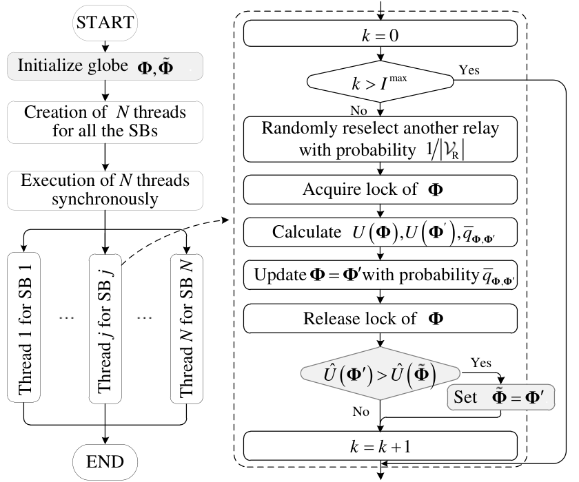
To this end, we propose a Markov-chain-guided multi-thread search algorithm (M-MTSA) as shown in Fig. 5. Inspired by Markov approximation [40], we first approximate (P1) by transforming it into a continuous convex optimization problem (P2) in the probability domain based on Log-Sum-Exp approximation and the conjugate function property. The decision variables in (P2) are the probability weights corresponding to all possible ${\mathbf{\Phi}}$. Ideally, the probability corresponding to the optimal strategy ${\mathbf{\Phi}}^{*}$ is remarkably close to one. Then, we construct a Markov chain with the state space as all possible ${\mathbf{\Phi}}$ and the stationary distribution as the optimal solution of (P2). During its execution, according to constraint (b), M-MTSA maintains $N$ threads for all the SUs, respectively. The partial strategy for thread $j$ serves as the $j$th column of ${\mathbf{\Phi}}$, a one-hot vector, which determines the selected relay for SU $j$. According to the transition rates of the Markov chain, the individual relays for the SUs are constantly and distributively updated with small inter-thread message passing overhead. By the careful design of transition rates, the Markov chain jumps to better strategies over time. Next, we detail the problem transformation, Markov chain construction, and M-MTSA design in Sections IV-D1-IV-D3, respectively.

References

- [1] J. Luettin, S. Monka, C. Henson, and L. Halilaj, “A survey on knowledge graph-based methods for automated driving,” in Iberoamerican Knowledge Graphs and Semantic Web Conference. Springer, 2022, pp. 16–31.
- [2] J. E. Kim, C. Henson, K. Huang, T. A. Tran, and W.-Y. Lin, “Accelerating road sign ground truth construction with knowledge graph and machine learning,” in Intelligent Computing. Springer, 2021, pp. 325–340.
- [3] L. Halilaj, I. Dindorkar, J. Lüttin, and S. Rothermel, “A knowledge graph-based approach for situation comprehension in driving scenarios,” in European Semantic Web Conference. Springer, 2021, pp. 699–716.
- [4] X. Liu, Z. Xu, Y. Meng, W. Wang, J. Xie, and Y. Li, “An elastic-segment-based V2V/V2I cooperative strategy for throughput enhancement,” IEEE Trans. Veh. Technol., vol. 71, no. 5, pp. 5272–5283, May 2022.
- [5] W. Weaver, “Recent contributions to the mathematical theory of communication,” ETC: a review of general semantics, pp. 261–281, 1953.
- [6] W. Yang, H. Du, Z. Liew, W. Y. B. Lim, Z. Xiong, D. Niyato, X. Chi, X. S. Shen, and C. Miao, “Semantic communications for 6G future Internet: Fundamentals, applications, and challenges,” IEEE Commun. Surv. Tutor., 2022.
- [7] W. Yang, Z. Q. Liew, W. Y. B. Lim, Z. Xiong, D. Niyato, X. Chi, X. Cao, and K. B. Letaief, “Semantic communication meets edge intelligence,” IEEE Wirel. Commun., vol. 29, no. 5, pp. 28–35, 2022.
- [8] C.-H. Lee, J.-W. Lin, P.-H. Chen, and Y.-C. Chang, “Deep learning-constructed joint transmission-recognition for internet of things,” IEEE Access, vol. 7, pp. 76 547–76 561, 2019.
- [9] H. Xie, Z. Qin, G. Y. Li, and B.-H. Juang, “Deep learning enabled semantic communication systems,” IEEE Trans. Signal Process., vol. 69, pp. 2663–2675, 2021.
- [10] Z. Weng, Z. Qin, and G. Y. Li, “Semantic communications for speech signals,” in ICC 2021-IEEE International Conference on Communications. IEEE, 2021, pp. 1–6.
- [11] H. Qiu, A. Ayara, and B. Glimm, “A knowledge architecture layer for map data in autonomous vehicles,” in 2020 IEEE 23rd International Conference on Intelligent Transportation Systems (ITSC). IEEE, 2020, pp. 1–6.
- [12] Z. Q. Liew, Y. Cheng, W. Y. B. Lim, D. Niyato, C. Miao, and S. Sun, “Economics of semantic communication system in wireless powered internet of things,” in ICASSP 2022-2022 IEEE International Conference on Acoustics, Speech and Signal Processing (ICASSP). IEEE, 2022, pp. 8637–8641.
- [13] L. Liu, M. Zhao, M. Yu, M. A. Jan, D. Lan, and A. Taherkordi, “Mobility-aware multi-hop task offloading for autonomous driving in vehicular edge computing and networks,” IEEE trans. Intell. Transp. Syst., vol. 24, no. 2, pp. 2169–2182, 2022.
- [14] H. Zhang, X. Zhang, and D. K. Sung, “An efficient cooperative transmission based opportunistic broadcast scheme in vanets,” IEEE Trans. Mob. Comput., 2021.
- [15] P. Kolios, V. Friderikos, and K. Papadaki, “Load balancing via store-carry and forward relaying in cellular networks,” in 2010 IEEE Global Telecommunications Conference (GLOBECOM). IEEE, 2010, pp. 1–6.
- [16] Y. Wang, Y. Liu, J. Zhang, H. Ye, and Z. Tan, “Cooperative store–carry–forward scheme for intermittently connected vehicular networks,” IEEE Trans. Veh. Technol., vol. 66, no. 1, pp. 777–784, Jan. 2016.
- [17] H. Xie and Z. Qin, “A lite distributed semantic communication system for internet of things,” IEEE J. Sel. Areas Commun., vol. 39, no. 1, pp. 142–153, 2020.
- [18] Q. Zhou, R. Li, Z. Zhao, C. Peng, and H. Zhang, “Semantic communication with adaptive universal transformer,” IEEE Wireless Commun. Lett., vol. 11, no. 3, pp. 453–457, 2021.
- [19] K. Lu, Q. Zhou, R. Li, Z. Zhao, X. Chen, J. Wu, and H. Zhang, “Rethinking modern communication from semantic coding to semantic communication,” IEEE Wirel. Commun., 2022.
- [20] M. Karimzadeh-Farshbafan, W. Saad, and M. Debbah, “Curriculum learning for goal-oriented semantic communications with a common language,” IEEE Trans. Commun., 2023.
- [21] C. K. Thomas and W. Saad, “Neuro-symbolic causal reasoning meets signaling game for emergent semantic communications,” arXiv preprint arXiv:2210.12040, 2022.
- [22] Y. Wang, M. Chen, T. Luo, W. Saad, D. Niyato, H. V. Poor, and S. Cui, “Performance optimization for semantic communications: An attention-based reinforcement learning approach,” IEEE J. Sel. Areas Commun., vol. 40, no. 9, pp. 2598–2613, 2022.
- [23] F. Zhou, Y. Li, X. Zhang, Q. Wu, X. Lei, and R. Q. Hu, “Cognitive semantic communication systems driven by knowledge graph,” in ICC 2022-IEEE International Conference on Communications. IEEE, 2022, pp. 4860–4865.
- [24] H. Seo, J. Park, M. Bennis, and M. Debbah, “Semantics-native communication with contextual reasoning,” IEEE Trans. Cogn., 2023.
- [25] K. Fall, “A delay-tolerant network architecture for challenged internets,” in Proceedings of the 2003 conference on Applications, technologies, architectures, and protocols for computer communications, 2003, pp. 27–34.
- [26] D. Wu, G. Zhu, and D. Zhao, “Adaptive carry-store forward scheme in two-hop vehicular delay tolerant networks,” IEEE Commun. Lett., vol. 17, no. 4, pp. 721–724, Apr. 2013.
- [27] S. H. Bouk, S. H. Ahmed, B. Omoniwa, and D. Kim, “Outage minimization using bivious relaying scheme in vehicular delay tolerant networks,” Wirel. Pers. Commun., vol. 84, no. 4, pp. 2679–2692, Apr. 2015.
- [28] O. Trullols-Cruces, M. Fiore, and J. Barcelo-Ordinas, “Cooperative download in vehicular environments,” IEEE Trans. Mob. Comput., vol. 11, no. 4, pp. 663–678, Apr. 2012.
- [29] J. Chen, A. Zafar, G. Mao, and C. Li, “On the achievable throughput of cooperative vehicular networks,” in 2016 IEEE International Conference on Communications (ICC). IEEE, 2016, pp. 1–7.
- [30] A. Agarwal and P. Kumar, “Capacity bounds for ad hoc and hybrid wireless networks,” ACM SIGCOMM COMP. COM., vol. 34, no. 3, pp. 71–81, Mar. 2004.
- [31] G. Zhu, L. Zhang, Y. Jiang, Y. Dang, H. Hou, P. Shen, M. Feng, X. Zhao, Q. Miao, S. A. A. Shah et al., “Scene graph generation: A comprehensive survey,” arXiv preprint arXiv:2201.00443, 2022.
- [32] W. Zhang, J. Chen, J. Li, Z. Xu, J. Z. Pan, and H. Chen, “Knowledge graph reasoning with logics and embeddings: Survey and perspective,” arXiv preprint arXiv:2202.07412, 2022.
- [33] P. Zhang, W. Xu, H. Gao, K. Niu, X. Xu, X. Qin, C. Yuan, Z. Qin, H. Zhao, J. Wei et al., “Toward wisdom-evolutionary and primitive-concise 6G: A new paradigm of semantic communication networks,” Engineering, vol. 8, pp. 60–73, 2022.
- [34] P. Wu, L. Ding, Y. Wang, and H. Zheng, “V2V-assisted V2I mmwave communication for cooperative perception with information value-based relay,” in 2021 IEEE Global Communications Conference (GLOBECOM). IEEE, 2021, pp. 1–6.
- [35] W. Zhang, Y. Chen, Y. Yang, X. Wang, Y. Zhang, X. Hong, and G. Mao, “Multi-hop connectivity probability in infrastructure-based vehicular networks,” IEEE Journal on Selected Areas in Communications, vol. 30, no. 4, pp. 740–747, 2012.
- [36] L. Su, Y. Niu, Z. Han, B. Ai, R. He, Y. Wang, N. Wang, and X. Su, “Content distribution based on joint V2I and V2V scheduling in mmwave vehicular networks,” IEEE Trans. Veh. Technol., vol. 71, no. 3, pp. 3201–3213, Mar. 2022.
- [37] L. Xu, Z. Yang, H. Wu, Y. Zhang, Y. Wang, L. Wang, and Z. Han, “Socially driven joint optimization of communication, caching, and computing resources in vehicular networks,” IEEE Trans. Wirel. Commun., vol. 21, no. 1, pp. 461–476, Jan. 2022.
- [38] S. K. Yoo, P. C. Sofotasios, S. L. Cotton, S. Muhaidat, F. J. Lopez-Martinez, J. M. Romero-Jerez, and G. K. Karagiannidis, “A comprehensive analysis of the achievable channel capacity in composite fading channels,” IEEE Access, vol. 7, pp. 34 078–34 094, 2019.
- [39] I. S. Gradshteyn and I. M. Ryzhik, Table of Integrals, Series, and Products Seventh Edition. USA: Elsevier, 2007.
- [40] M. Chen, S. C. Liew, Z. Shao, and C. Kai, “Markov approximation for combinatorial network optimization,” IEEE Trans. Inf. Theory, vol. 59, no. 10, pp. 6301–6327, Oct. 2013.
- [41] S. Boyd, S. P. Boyd, and L. Vandenberghe, Convex optimization. Cambridge university press, 2004.
- [42] O. Ibe, Markov processes for stochastic modeling. Newnes, 2013.
- [43] C. Chen, J. Hu, T. Qiu, M. Atiquzzaman, and Z. Ren, “CVCG: Cooperative V2V-aided transmission scheme based on coalitional game for popular content distribution in vehicular ad-hoc networks,” IEEE Trans. Mob. Comput., vol. 18, no. 12, pp. 2811–2828, 2018.
![[Uncaptioned image]](/html/2307.15284/assets/wantingyang.jpeg) |
Wanting Yang received the B.S. degree and the Ph.D. degree from the Department of Communications Engineering, Jilin University, Changchun, China, in 2018 and 2023, respectively. She was a visiting student at Singapore University of Technology and Design from 2021 to 2022, sponsored by the Chinese Scholarship Council. She served as Technical Programme Committee member in flagship conferences, such as WCNC, Globecom, and VTC. Her research interests include wireless communications, predictive resource allocation, semantic communication, learning, martingale and URLLC. |
![[Uncaptioned image]](/html/2307.15284/assets/xuefenchi.jpeg) |
Xuefen Chi received the B.Eng. degree in applied physics from the Beijing University of Posts and Telecommunications, Beijing, China, in 1984, and the M.S. and Ph.D. degrees from the Changchun Institute of Optics, Fine Mechanics and Physics, Chinese Academy of Sciences, Changchun, China, in 1990 and 2003, respectively. She was a Visiting Scholar with the Department of Computer Science, Loughborough University, U.K., in 2007, and the School of Electronics and Computer Science, University of Southampton, Southampton, U.K., in 2015. She is currently a Professor with the Department of Communications Engineering, Jilin University, China. Her research interests include machine-type communications, indoor visible light communications, random access algorithms, delay-QoS guarantees, and network modeling theory and its applications. |
![[Uncaptioned image]](/html/2307.15284/assets/linlinzhao.jpeg) |
Linlin Zhao received the B.Eng., M.S., and Ph.D. degrees from the Department of Communications Engineering, Jilin University, Changchun, China, in 2009, 2012, and 2017, respectively. From 2017 to 2019, she was a Post-Doctoral Researcher with the Department of Communications Engineering, Jilin University. She is currently an Associate Professor with the Department of Communications Engineering, Jilin University, and a Post-Doctoral Research Fellow with the State Key Laboratory of Internet of Things for Smart City, University of Macau. Her current research interests include throughput optimal random access algorithms, resource allocation schemes, and delay and reliability analysis and optimization, especially for reliability analysis of ultra-reliable low-latency communications. She was a recipient of the Best Ph.D. Thesis Award of Jilin University in 2017, and acquired the Macau Young Scholars Program in 2019. She has served as the Registration Co-Chair for IEEE ICCC 2019. |
![[Uncaptioned image]](/html/2307.15284/assets/zehuixiong.jpeg) |
Zehui Xiong is currently an Assistant Professor at Singapore University of Technology and Design, and also an Honorary Adjunct Senior Research Scientist with Alibaba-NTU Singapore Joint Research Institute, Singapore. He received the PhD degree in Nanyang Technological University (NTU), Singapore. He was the visiting scholar at Princeton University and University of Waterloo. His research interests include wireless communications, Internet of Things, blockchain, edge intelligence, and Metaverse. He has published more than 200 research papers in leading journals and flagship conferences and many of them are ESI Highly Cited Papers. He has won over 10 Best Paper Awards in international conferences and is listed in the World’s Top 2% Scientists identified by Stanford University. He is now serving as the editor or guest editor for many leading journals including IEEE Journal on Selected Areas in Communications, IEEE Transactions on Vehicular Technology, IEEE Internet of Things Journal, IEEE Transactions on Cognitive Communications and Networking, and IEEE Transactions on Network Science and Engineering. He is the recipient of IEEE Early Career Researcher Award for Excellence in Scalable Computing, IEEE Technical Committee on Blockchain and Distributed Ledger Technologies Early Career Award, IEEE Internet Technical Committee Early Achievement Award, IEEE TCSVC Rising Star Award, IEEE TCI Rising Star Award, IEEE TCCLD Rising Star Award, IEEE Best Land Transportation Paper Award, IEEE CSIM Technical Committee Best Journal Paper Award, IEEE SPCC Technical Committee Best Paper Award, IEEE VTS Singapore Best Paper Award, Chinese Government Award for Outstanding Students Abroad, and NTU SCSE Best PhD Thesis Runner-Up Award. He is now serving as the Associate Director of Future Communications R&D Programme. In 2023, he was featured on the list of Forbes Asia 30 under 30. |
![[Uncaptioned image]](/html/2307.15284/assets/wenchaojiang.jpeg) |
Wenchao Jiang received the Ph.D. degree from the Department of Computer Science and Engineering, University of Minnesota Twin Cities, in 2019. He is currently an Assistant Professor with the Pillar of Information System Technology and Design, Singapore University of Technology and Design. His research interests include the Internet of Things, wireless and low-power embedded networks, and mobile computing. |