Is this model reliable for everyone?
Testing for strong calibration
Abstract
In a well-calibrated risk prediction model, the average predicted probability is close to the true event rate for any given subgroup. Such models are reliable across heterogeneous populations and satisfy strong notions of algorithmic fairness. However, the task of auditing a model for strong calibration is well-known to be difficult—particularly for machine learning (ML) algorithms—due to the sheer number of potential subgroups. As such, common practice is to only assess calibration with respect to a few predefined subgroups. Recent developments in goodness-of-fit testing offer potential solutions but are not designed for settings with weak signal or where the poorly calibrated subgroup is small, as they either overly subdivide the data or fail to divide the data at all. We introduce a new testing procedure based on the following insight: if we can reorder observations by their expected residuals, there should be a change in the association between the predicted and observed residuals along this sequence if a poorly calibrated subgroup exists. This lets us reframe the problem of calibration testing into one of changepoint detection, for which powerful methods already exist. We begin with introducing a sample-splitting procedure where a portion of the data is used to train a suite of candidate models for predicting the residual, and the remaining data are used to perform a score-based cumulative sum (CUSUM) test. To further improve power, we then extend this adaptive CUSUM test to incorporate cross-validation, while maintaining Type I error control under minimal assumptions. Compared to existing methods, the proposed procedure consistently achieved higher power in simulation studies and more than doubled the power when auditing a mortality risk prediction model.
1 Introduction
Calibration is a fundamental measure of model reliability: a risk prediction model is calibrated for a subgroup if the average predicted probability corresponds to the observed event rate. When decisions are made using absolute risk thresholds—as is common in medicine [15]—calibration has also been shown to directly impact the utility of a model [44]. However, machine learning (ML) algorithms are typically trained to optimize average performance and can be poorly calibrated in particular subgroups [5, 1], leading to concerns regarding their robustness and fairness. In fact, performance can be particularly low for subgroups defined by interactions of multiple variables (e.g. race and gender), an issue known as intersectionality [4]. Ideally, a risk prediction model is “strongly” calibrated, in that it is calibrated for all individuals or, equivalently, all possible subgroups [45, 53].
Unfortunately, achieving or even verifying strong calibration is challenging due to the curse of dimensionality: as the number of variables grows, the subgroups—and thus the number of observations per subgroup—get smaller. As such, much of this research has been focused on “moderate” calibration, which only require calibration with respect to a small set of predefined subgroups [3, 42, 20, 22, 23, 31, 7]. These methods are widely used among practitioners, given their ease of use and applicability to small datasets. With the recent interest in algorithmic fairness and model reliability, many recent works have sought to achieve stronger forms of calibration, either by identifying subgroups that require revision [6, 11] or revising the model directly [21, 27, 33]. However, these methods are either meant to be exploratory or only provide statistical guarantees when the number of observations is sufficiently large. The minimum sample size is typically at least tens or even hundreds of thousands of observations, which is often unrealistic in many settings.
Rather than tackling the difficult task of subgroup identification or model revision, we instead consider the problem of testing if there exists any poorly calibrated subgroup. This is much more feasible in settings with limited data or lower signal-to-noise ratios, and still answers the important yes/no question “Is this ML algorithm reliable for everyone?” Moreover, the answer to this question can help decide if more sophisticated data-hungry procedures are necessary.
We formalize this as the following hypothesis test. Let be the risk prediction algorithm and be the true event rate over some domain , where is the number of variables. For some pre-specified tolerance level , define the poorly calibrated subgroup as The hypothesis test checks if the set is too large, i.e.
| (1) | ||||
from some minimally acceptable prevalence . [24] considers a similar hypothesis test, but only for the univariate case () and where . Unfortunately, it is unclear how to extend their proposal to settings with larger or .
In settings with larger , the most relevant works are [26] and [52] from the goodness-of-fit (GOF) testing literature. Although GOF tests technically answer a different question from (1), it is relatively straightforward to extend these methods to test for strong calibration. To address the curse of dimensionality, both procedures perform sample-splitting: a portion of the data is used to train a random forest (RF) to predict the residuals and the remaining data are used to test for GOF with respect to the learned residual model. The difference between [26] and [52] is primarily in the second step. The former assesses the association between the predicted and observed residuals with respect to the entire population through a score test, so it fails to reflect subpopulation structure. The latter bins observations with similar predicted residuals and performs a Chi-squared test, but no information is borrowed across bins and the procedure can be highly sensitive to the number of bins. As such, there are a number of limitations with these works. First, these methods are not well-suited for settings where only a subgroup is poorly calibrated, particularly when this subgroup is small. In addition, both papers only use RFs to model the residuals, but we show that RFs are weak at extracting the remaining signal after fitting a tree-based risk prediction model. Instead, it is important to consider a diverse pool of candidate residual models. Also, there are no extensions of these methods that use cross-validation (CV) while maintaining Type I error control. Finally, to fit the residual model, both procedures perform further sample splitting to tune the hyperparameters. This can be noisy in small sample sizes and lead to an suboptimal choice of hyperparameters. It is also computationally expensive when combined with CV.
We introduce a more powerful testing procedure for strong calibration motivated with the following insight: if observations are ordered by their predicted residuals, we expect the association between the observed and predicted residuals to drop somewhere along this sequence if a poorly calibrated subgroup exists. Our key contributions are (i) we show how reframing the problem of detecting a poorly calibrated subgroup into that of changepoint detection substantially improves power because the changepoint structure closely mimics the true subpopulation structure; (ii) we demonstrate how additional gains in power and computational efficiency can be made by fitting a pool of candidate residual models and performing a suite of structural change tests; (iii) we incorporate CV into the procedure to further improve power, while maintaining Type I error control under much weaker assumptions than prior works; and (iv) we provide visualization tools to aid model diagnosis. In experiments, the proposed procedure significantly outperforms existing methods. Code is available at https://github.com/jjfeng/testing_strong_calibration.
1.1 Related works
Individual/metric fairness. Strong calibration of a ML algorithm is only one approach to measuring model fairness. Other common measures of algorithmic fairness are concerned with statistical parity or balance of error rates between subgroups [19, 36]. Similar to the critiques of moderate calibration, group-wise equality in error rates has been critized for being too coarse [10]. Recent works have aimed for individual or metric fairness to ensure similar performance between similar individuals [25, 40], and hypothesis tests for evaluating individual fairness have been developed [51, 34]. However, unlike the proposed procedure, these methods assume a similarity metric is known a priori, which corresponds to prespecifying the subgroup structure.
Conformal inference. Recent works have highlighted how the coverage rate guarantees from conformal inference procedures can be used to calibrate risk prediction algorithms [48, 35]. Ordinary conformal inference procedures only guarantee marginal coverage rates [47], which satisfy notions of weak calibration [45]. More recent works have extended these methods to provide guarantees with respect to predefined subgroups [46, 28, 39] and weighted neighborhoods [18]. Taking such guarantees to the limit, [14] proved that it is impossible for a non-trivial procedure to guarantee uniform conditional coverage rates. Our ability to test for strong calibration does not contradict this impossibility result and provides instead a complementary (and perhaps more positive) result. Because hypothesis tests start from the opposite angle of “innocent until proven guilty,” we can at least determine if there is sufficient evidence that a given model fails to satisfy strong calibration.
Distributionally robust optimization (DRO). Much of DRO is concerned with training models that minimize the worst-case performance over some set of distributional perturbations [2, 9, 8]. Based on these ideas, recent works propose to estimate the worst-case performance of a given ML algorithm over all subgroups with size [41, 30]. [41] is closest in spirit to this work, in that it performs statistical inference to output confidence intervals (CI). In fact, it similarly splits the data to estimate a model of the ML algorithm’s error on one partition and assess worst-case performance on the other partition. Nevertheless, the method differs in that it requires much larger sample sizes, to be bounded away from zero, and the error model to converge at a fast enough rate. In contrast, our proposed procedure is suitable for smaller sample sizes, can test for arbitrarily small subgroups, provides assumption-free, finite-sample Type I error control when performing a single sample-split, and requires much weaker assumptions to establish asymptotic Type I error control when using CV.
2 Method
For ease of exposition, we begin with the one-sided testing problem where we replace with the one-sided violation set . The first step is to reformulate the hypothesis test as a score test. In the main text of this paper, we focus on the test where . In the Appendix, we describe how the proposed procedure can be easily extended to address non-zero .
Let be the class of bounded non-negative real-valued functions. For a given , define a working model for the structural change of the log odds (logit) to be
| (2) |
where and is a projection into the range of valid probabilities . The gradient of the log likelihood, also known as the score, at is equal to
| (3) |
In the set , the expected score is positive if is positive. Outside of this set, the expected score is non-positive. As such, we will refer to as a detector. We can rewrite the one-sided hypothesis test in terms of the maximum expected score over detectors in , i.e.
| (4) | ||||
In practice, it is computationally infeasible to test the entire set . Instead, we will generate a subset to replace in (4), resulting in a restricted score test. Thus a procedure with Type I error control for a restricted score test also satisfies Type I error control for (4).
In the following sections, we introduce the testing procedure using single sample-split, extend it to incorporate CV, and finally extend it to the two-sided setting.
2.1 Sample-splitting
Suppose the audit data are composed of independent and identically distributed (IID) observations with variables and binary outcome for . The outline for the sample-splitting procedure is as follows. Let the first observations form a training partition and the remaining observations form a test partition. Using the training data, we generate a set of candidate detectors across different hyperparameter settings . Using the test data, we calculate the maximum empirical score over the set of candidate detectors as our test statistic, i.e.
| (5) |
We reject the null hypothesis if exceeds the critical value defined in the theorem below.
As described below, we use a simple Monte Carlo procedure to calculate the critical value which, unlike existing tests for model calibration, provides finite-sample Type I error control. In particular, using a coupling argument, we prove that the distribution of the test statistic is stochastically largest at the boundary of the null hypothesis space where . Proofs for all the theoretical results are in the Appendix.
Theorem 1.
Let be the binary random variable with probability . By setting to be the quantile of
| (6) |
the Type I error of the sample-splitting test is controlled at level .
Given the Type I error guarantee, the key question is how to construct a set of detectors that maximizes power. As motivation, suppose we were only allowed to generate a single detector . Per [43], the local asymptotic power of the test with respect to is determined by the ratio
| (7) |
Let denote the expected residuals. Given the constraint that detectors must be non-negative, the numerator is maximized by . To maximize the ratio, we can tune over the broader class of detectors for , which also reflects our interest in observations with the largest values of . This family of detectors has another advantage in practice, where is unknown and must be estimated. Generating detectors based on an estimate of the expected residuals, the expected score is large as long as thresholding on the predicted residuals isolates a subset of observations with large , even if the predicted residuals are not accurate for the entire population.
Given this motivation, we propose the following procedure for generating detectors. Suppose one has a set of candidate algorithms (e.g. random forests and neural networks) for estimating the residuals, indexed by the set of hyperparameters . We fit residual models for each on the training partition, and construct the set of detectors
| (8) |
The test statistic can now be rewritten as
| (9) |
Notice that the inner summation corresponds exactly to the score-based cumulative sum (CUSUM) test statistic, which is typically used to detect changepoints along a single axis [16, 17, 12]. So our procedure can be viewed as performing changepoint detection along data-adaptively defined axes , where the null hypothesis of each changepoint test is that the mean score is uniformly non-negative and the alternative is that there is some point after which the mean score is positive.
Leveraging this connection with the changepoint literature, we can visualize the test using “control charts,” which are typically used to visualize changepoint detection procedures along a single dimension [37, 13]. As shown in the example in Figure 1, each curve corresponds to the cumulative score when observations are ordered by their predicted residuals, and the maximum value attained across all curves corresponds to the test statistic. Large positive slopes correspond to subgroups where the model is very poorly calibrated, whereas flat or negative slopes correspond to subgroups where model calibration is mostly within the desired tolerance. The location of the peak indicates the size of the poorly calibrated subgroup detected by the procedure. Thus the shape of the curve provides insight into the nature of the poorly calibrated subgroup.
Finally, one may ask (i) how many candidate residual models should one fit and (ii) how much data should one dedicate to training the residual models? These questions concern two tradeoffs. More residual models increase our chance of finding a changepoint but require more stringent multiplicity correction. Also, allocating more data to training can increase the accuracy of the residual models but reduces the sample size available for testing. We clarify the answer to these two questions in the following result. Note that denote positive constants below.
Theorem 2.
Consider any and . Suppose is chosen so that Conditional on the event that
| (10) |
statistical power is lower bounded by
| (11) |
where is the number of hyperparameters.
The lower bound in (11) states that the number of hyperparameters impacts power only through a logarithmic term, which justifies our approach of testing a suite of residual models. In contrast, existing methods test only a single residual model [26, 52], which is tuned using CV within the training partition. In settings with limited amounts of audit data, CV tends to overfit and select a suboptimal detector, leading to lower power. Moreover, this procedure is very computationally expensive when combined with CV, because one would have to perform CV within CV.
Second, the numerator in (11) grows linearly with the amount of test data and slowly with the amount of training data. This highlights an interesting “phase change” in how much data one should allocate to training versus testing. One should allocate just enough training data so that (10) is satisfied with high probability (note that many ML algorithms have convergence rates of this form) and dedicate the rest to testing.
2.2 -fold Cross-validation
We now extend the sample-splitting procedure to use CV to further improve power. The technical challenge is how to maintain Type I error control, despite the correlation between estimators across folds. Prior works provide only ad-hoc solutions [52] or assume estimators converge to the oracle sufficiently fast [41]. Here we present a procedure that requires very minimal assumptions.
We extend the sample-splitting procedure as follows. Partition the audit data into folds for . For each , let denote the estimated residual model using data in all but the -th fold for . The CV test statistic is defined as
| (12) |
To establish Type I error control, we only require the following uniform convergence assumption.
Assumption 1.
For a given and , define as the average detector estimated from folds of a dataset with observations. That is, , where the expectation is with respect to the estimated residual models. Suppose that
| (13) |
Under this assumption, we prove that one can essentially treat the estimated residual models as fixed and use the same Monte Carlo procedure as before to calculate the critical value. The only difference is that we control the Type I error rate asymptotically, rather than in finite samples.
2.3 Extension to the two-sided test
Finally, we extend the procedure to test the two-sided null hypothesis. The key difference is that rather than ordering observations by their predicted residuals, we now order observations by the magnitude of the predicted residuals. For ease of exposition, we only describe the sample-splitting procedure for the two-sided setting. The same ideas are used to extend the CV procedure.
Following the same logic as before, we begin with restating the two-sided hypothesis test in terms of a score test. Let refer to the set of bounded functions, removing the prior restriction of non-negativity. For a given , the working model for structural change is now where is the sign of and zero if , and . Thus we can reframe (1) as
| (14) | ||||
As before, we will instead perform a restricted score test by generating candidate detectors given a set of hyperparameters . More specifically, for each , we fit residual models that estimate if , if , and zero otherwise. We then generate detectors for . Consequently, the test statistic in the two-sided setting is the maximum of the score-based CUSUM statistics where observations are ordered by the absolute predicted residuals, i.e.
| (15) |
To calculate the critical value, we must modify the Monte Carlo procedure. Unlike the one-sided setting, it is no longer straightforward to determine the null distribution whose test statistic is stochastically largest, because estimated models may disagree on the sign of the expected residual. As such, we set the critical value to the quantile of a modified statistic that upper bounds (15). More specifically, for each , we sample two binary outcomes with marginal probabilities and . For each model , we calculate a “bounding” CUSUM statistic by selecting the outcome generated with probability if the predicted residual is positive and if the predicted residual is negative. The modified statistic is the maximum of these bounding CUSUM statistics. This procedure, formally described below, ensures finite-sample Type I error control.
Theorem 4.
Let for be IID standard uniform random variables. Define Define using (15) but replacing with . Set the critical value to the quantile of , For the two-sided hypothesis test, the sample-splitting procedure that rejects the null when controls the Type I error at level .
2.4 Variable importance plots
In addition to control charts, we can use variable importance (VI) plots to gain insight into potential reasons for model miscalibration. Here we consider a simple procedure using permutation VI to compute how important each variable is for detecting a poorly calibrated subgroup. (Future work may consider more sophisticated VI measures such as using Shapley values [32, 50].) For each variable, we permute its values and calculate the change in the test statistic. The importance of that variable is defined as the drop in the test statistic, where a larger drop indicates a more important variable. We emphasize that this definition of VI is not the same as ordinary VI measures that quantify how useful a variable is to a model’s average performance. Ordinary VI measures describe the majority group and are not meant to characterize poorly calibrated subgroups.
3 Simulations
| Chi-squared tests | Score-based tests | |
|---|---|---|
| Prespecified axis | Hosmer-Lemeshow: ChiSq | Score test for Platt scaling: Score |
| Data-adaptive axes | Based on [52]: AdaptiveChiSq | Based on [26]: AdaptiveScoreSimple |
| Proposed: AdaptiveScoreCUSUM |
We begin with a simulation study comparing the proposed procedure (AdaptiveScoreCUSUM) to four procedures: the Hosmer-Lemeshow test (ChiSq) [29], a score test based on Platt scaling (Score) [38], an adaptive Chi-squared test that extends [52] (AdaptiveChiSq), and an adaptive score test that extends [26] (AdaptiveScoreSimple). The two comparator score tests can be viewed as special cases of our procedure. Score implements a score-based CUSUM test with respect to the logistic recalibration model (2) along the prespecified axis . This test is not data-adaptive, so it does not require sample-splitting. AdaptiveScoreSimple is implemented to be almost the same as ours except, following [26], we do not explicitly create subgroup detectors and fix . The procedures can be categorized with respect to the 2x2 grid shown in Table 1, where the rows correspond to test procedures that prespecify versus adaptively define axes, and columns correspond to procedures that run Chi-squared versus score tests. For tests that prespecify axes, we follow standard practice and use the single axis . For all methods, we use the proposed Monte Carlo procedure to calculate critical values and control Type I error.
For the Chi-squared tests, we present results for when the data are divided into 2 versus 10 bins. We had also tested bin numbers in between, but the performance was similar or worse. Because Chi-squared tests are traditionally designed to test hypotheses with a tolerance of , we modified the test statistic to test non-zero tolerances.
The data-adaptive tests were implemented using 4-fold CV and made to be as comparable as possible. To this end, we extend and unify tests in [26] and [52] using our framework. We fit residual models using RFs and kernel logistic regression across various hyperparameter settings. The detectors use as input variables as well as the predicted logit from the risk prediction algorithm.
We simulate data as follows. Covariates were independently sampled from Uniform. The outcome is sampled with the log odds as
| (16) |
The Appendix includes additional simulation details and results as well as a second simulation study verifying Type I error control of the proposed procedure.


We test the two-sided null hypothesis (1) for two algorithms: a logistic regression model (LR) that incorrectly assumes the logit is linear with respect to the variables and a RF. A RF is not misspecified, but it must approximate the piecewise linear relationship and thus converges slowly to the true risk. For tolerance levels , and 0.075, the poorly calibrated subgroups had prevalences 0.60, 0.45, and 0.25 for the LR model and 0.8, 0.5, and 0.3 for the RF model, respectively.
AdaptiveScoreCUSUM consistently outperformed other methods across all settings (Figure 2). Tests that relied on a prespecified axis performed the worst. Adaptive score-based tests demonstrated major improvements on the adaptive chi-squared test; in certain settings, power more than doubles. This improvement is particularly evident at higher tolerance levels, where the poorly calibrated subgroup is smaller and it becomes even more important to extract much signal from the data as possible. AdaptiveScoreCUSUM offered the biggest improvements over AdaptiveScoreSimple in smaller sample sizes, because the residual models can be quite inaccurate in such settings and, by restricting to , AdaptiveScoreSimple has difficulty isolating regions with poor calibration.
If we investigate the results from AdaptiveScoreCUSUM for the LR model, we find that the random forest-based detector maximized the test statistics in a majority of the cases. This is unsurprising, given that the subgroup structure in equation (16) matches the structure learned by recursive partitioning. Moreover, the VI plots show that the detection models indeed recoreved the misspecified subgroup, as the variables , and , were assigned the highest importance.
Similarly, we investigate test results for the RF model. As the audit dataset increased, the test statistic was more often maximized by kernel logistic regression. This illustrates how RFs are not very powerful for detecting miscalibration of a RF, because we have already extracted most of the signal from the data using recursive partitioning. Kernel logistic regression uses an entirely different approach, so it is better at extracting the remaining signal. From the associated VI plots, we see that , , and are now the most important for detecting poor calibration. This likely reflects the fact that kernel logistic regression converges faster than RF to the true probabilities in certain regions.
4 Predicting one-year mortality using Electronic Health Record data
We now compare the proposed procedure to existing methods in an analysis of Electronic Health Record (EHR) data from the Zuckerberg San Francisco General Hospital (ZSFG). We trained RFs to predict one-year mortality using data from 2019 to 2022. Input features to the RF included 31 demographic variables as well as ICD-10 diagnosis codes from the patient’s record. Across 40 replicates, we randomly assigned 250,000 patients to train the RF and randomly selected observations for testing strong calibration. We tested the two one-sided null hypotheses separately to differentiate between over- and under-estimation of the mortality rate. For added interpretability, we tested for strong calibration with respect to only the demographic variables.
Figure 3 shows that there is strong evidence that the RF model under-estimates the true risks and a lack of evidence of over-estimation. The rejection rate of AdaptiveScoreCUSUM reached 100%, which was more than five times higher than that of other methods. Similar to that in our simulation study, we again find that kernel logistic regression was most often selected as the maximizer of the test statistic. Analyzing the shape of the CUSUM plot from a sample replicate, we see that there is a sharp increase in the cumulative score process, and then a large drop. This suggests that there is a small subgroup identified by the kernel logistic model that is very poorly calibrated. VI plots further suggest that the most important variables that characterize this poorly calibrated group are age and the original risk prediction. Based on these findings, we plotted the calibration curves stratified by age and indeed find that subjects with under-estimated risks are defined by the intersection of patients under 60 years old and with risk predictions over 40%. Diagnostic plots like these can help model developers better understand where their algorithm is unreliable, which can be used to restrict model usage to certain subgroups, inform model revision, and more.


5 Discussion
We have presented an adaptive score-based CUSUM procedure for testing if a given ML algorithm is poorly calibrated for some subgroup. As shown in the empirical experiments, the procedure vastly outperforms existing methods. The key insight of this method is that if one has an estimate of expected residuals at each observation, we can transform the problem of subgroup detection to one of changepoint detection. Ordering observations by their predicted residuals, we should expect to see a change in the association between the observed and predicted residuals. Using a changepoint formulation, we can fully leverage the natural ordering of the data and the information learned by the estimated residual models, and avoid unnecessary binning of the data. Finally, we showed how accompanying control charts and VI plots can help model diagnostics and inform model revision.
Acknowledgments
We thank Adarsh Subbaswamy and Karen Feng for helpful discussions and suggestions. We are grateful to Lucas Zier for sharing the ZSFG dataset.
This work was supported by the Food and Drug Administration (FDA) of the U.S. Department of Health and Human Services (HHS) as part of a financial assistance award Center of Excellence in Regulatory Science and Innovation grant to University of California, San Francisco (UCSF) and Stanford University, U01FD005978 totaling $79,250 with 100% funded by FDA/HHS. The contents are those of the author(s) and do not necessarily represent the official views of, nor an endorsement, by FDA/HHS, or the U.S. Government.
References
- Barda et al. [2021] Noam Barda, Gal Yona, Guy N Rothblum, Philip Greenland, Morton Leibowitz, Ran Balicer, Eitan Bachmat, and Noa Dagan. Addressing bias in prediction models by improving subpopulation calibration. J. Am. Med. Inform. Assoc., 28(3):549–558, March 2021. URL http://dx.doi.org/10.1093/jamia/ocaa283.
- Ben-Tal et al. [2013] Aharon Ben-Tal, Dick den Hertog, Anja De Waegenaere, Bertrand Melenberg, and Gijs Rennen. Robust solutions of optimization problems affected by uncertain probabilities. Management Science, 59(2):341–357, 2013. doi: 10.1287/mnsc.1120.1641. URL https://doi.org/10.1287/mnsc.1120.1641.
- Brown et al. [1975] R L Brown, J Durbin, and J M Evans. Techniques for testing the constancy of regression relationships over time. J. R. Stat. Soc. Series B Stat. Methodol., 37(2):149–192, 1975. URL http://www.jstor.org/stable/2984889.
- Buolamwini and Gebru [2018] Joy Buolamwini and Timnit Gebru. Gender shades: Intersectional accuracy disparities in commercial gender classification. In Sorelle A Friedler and Christo Wilson, editors, Proceedings of the 1st Conference on Fairness, Accountability and Transparency, volume 81 of Proceedings of Machine Learning Research, pages 77–91, New York, NY, USA, 2018. PMLR. URL http://proceedings.mlr.press/v81/buolamwini18a.html.
- Chatterjee et al. [2016] Nilanjan Chatterjee, Jianxin Shi, and Montserrat García-Closas. Developing and evaluating polygenic risk prediction models for stratified disease prevention. Nat. Rev. Genet., 17(7):392–406, July 2016. URL http://dx.doi.org/10.1038/nrg.2016.27.
- Chung et al. [2019] Yeounoh Chung, Tim Kraska, Neoklis Polyzotis, Ki Hyun Tae, and Steven Euijong Whang. Slice finder: Automated data slicing for model validation. In 2019 IEEE 35th International Conference on Data Engineering (ICDE), pages 1550–1553, April 2019. URL http://dx.doi.org/10.1109/ICDE.2019.00139.
- DiCiccio et al. [2020] Cyrus DiCiccio, Sriram Vasudevan, Kinjal Basu, Krishnaram Kenthapadi, and Deepak Agarwal. Evaluating fairness using permutation tests. In Proceedings of the 26th ACM SIGKDD International Conference on Knowledge Discovery & Data Mining, KDD ’20, pages 1467–1477, New York, NY, USA, August 2020. Association for Computing Machinery. URL https://doi.org/10.1145/3394486.3403199.
- Duchi et al. [2022] John Duchi, Tatsunori Hashimoto, and Hongseok Namkoong. Distributionally robust losses for latent covariate mixtures. Oper. Res., September 2022. URL https://doi.org/10.1287/opre.2022.2363.
- Duchi and Namkoong [2021] John C Duchi and Hongseok Namkoong. Learning models with uniform performance via distributionally robust optimization. The Annals of Statistics, 49(3):1378–1406, June 2021. URL https://projecteuclid.org/journals/annals-of-statistics/volume-49/issue-3/Learning-models-with-uniform-performance-via-distributionally-robust-optimization/10.1214/20-AOS2004.full.
- Dwork et al. [2012] Cynthia Dwork, Moritz Hardt, Toniann Pitassi, Omer Reingold, and Richard Zemel. Fairness through awareness. In Proceedings of the 3rd Innovations in Theoretical Computer Science Conference, ITCS ’12, pages 214–226, New York, NY, USA, January 2012. Association for Computing Machinery. URL https://doi.org/10.1145/2090236.2090255.
- Eyuboglu et al. [2022] Sabri Eyuboglu, Maya Varma, Khaled Kamal Saab, Jean-Benoit Delbrouck, Christopher Lee-Messer, Jared Dunnmon, James Zou, and Christopher Re. Domino: Discovering systematic errors with Cross-Modal embeddings. International Conference on Learning Representations, May 2022. URL https://openreview.net/forum?id=FPCMqjI0jXN.
- Feng et al. [2022a] Jean Feng, Alexej Gossmann, Gene Pennello, Nicholas Petrick, Berkman Sahiner, and Romain Pirracchio. Monitoring machine learning (ML)-based risk prediction algorithms in the presence of confounding medical interventions. November 2022a. URL http://arxiv.org/abs/2211.09781.
- Feng et al. [2022b] Jean Feng, Rachael V Phillips, Ivana Malenica, Andrew Bishara, Alan E Hubbard, Leo A Celi, and Romain Pirracchio. Clinical artificial intelligence quality improvement: towards continual monitoring and updating of AI algorithms in healthcare. npj Digital Medicine, 5(1):1–9, May 2022b. URL https://www.nature.com/articles/s41746-022-00611-y.
- Foygel Barber et al. [2021] Rina Foygel Barber, Emmanuel J Candès, Aaditya Ramdas, and Ryan J Tibshirani. The limits of distribution-free conditional predictive inference. Inf Inference, 10(2):455–482, June 2021. URL https://academic.oup.com/imaiai/article-pdf/10/2/455/38549621/iaaa017.pdf.
- Goff et al. [2014] David C. Goff, Donald M. Lloyd-Jones, Glen Bennett, Sean Coady, Ralph B. D’Agostino, Raymond Gibbons, Philip Greenland, Daniel T. Lackland, Daniel Levy, Christopher J. O’Donnell, Jennifer G. Robinson, J. Sanford Schwartz, Susan T. Shero, Sidney C. Smith, Paul Sorlie, Neil J. Stone, and Peter W. F. Wilson. 2013 acc/aha guideline on the assessment of cardiovascular risk. Circulation, 129(25_suppl_2):S49–S73, 2014. doi: 10.1161/01.cir.0000437741.48606.98. URL https://www.ahajournals.org/doi/abs/10.1161/01.cir.0000437741.48606.98.
- Gombay [2003] Edit Gombay. Sequential Change-Point detection and estimation. Seq. Anal., 22(3):203–222, January 2003. URL https://doi.org/10.1081/SQA-120025028.
- Gombay [2017] Edit Gombay. Editor’s special invited paper: On the efficient score vector in sequential monitoring. Sequential Analysis, 36(4):435–466, October 2017. URL https://doi.org/10.1080/07474946.2017.1394728.
- Guan [2023] Leying Guan. Localized conformal prediction: a generalized inference framework for conformal prediction. Biometrika, 110(1):33–50, February 2023. URL https://academic.oup.com/biomet/article-pdf/110/1/33/49160126/asac040.pdf.
- Hardt et al. [2016] Moritz Hardt, Eric Price, Eric Price, and Nati Srebro. Equality of opportunity in supervised learning. In D D Lee, M Sugiyama, U V Luxburg, I Guyon, and R Garnett, editors, Advances in Neural Information Processing Systems 29, pages 3315–3323. Curran Associates, Inc., 2016. URL http://papers.nips.cc/paper/6374-equality-of-opportunity-in-supervised-learning.pdf.
- Hawkins [1991] Douglas M Hawkins. Diagnostics for use with regression recursive residuals. Technometrics, 33(2):221–234, 1991. URL http://www.jstor.org/stable/1269048.
- Hebert-Johnson et al. [2018] Ursula Hebert-Johnson, Michael Kim, Omer Reingold, and Guy Rothblum. Multicalibration: Calibration for the (Computationally-Identifiable) masses. International Conference on Machine Learning, 80:1939–1948, 2018. URL https://proceedings.mlr.press/v80/hebert-johnson18a.html.
- Hosmer et al. [1997] D W Hosmer, T Hosmer, S Le Cessie, and S Lemeshow. A comparison of goodness-of-fit tests for the logistic regression model. Stat. Med., 16(9):965–980, May 1997. URL http://dx.doi.org/10.1002/(sici)1097-0258(19970515)16:9<965::aid-sim509>3.0.co;2-o.
- Hosmer and Hjort [2002] David W Hosmer and Nils Lid Hjort. Goodness-of-fit processes for logistic regression: simulation results. Stat. Med., 21(18):2723–2738, September 2002. URL http://dx.doi.org/10.1002/sim.1200.
- Hudson et al. [2021] Aaron Hudson, Marco Carone, and Ali Shojaie. Inference on function-valued parameters using a restricted score test. May 2021. URL http://arxiv.org/abs/2105.06646.
- Ilvento [2020] Christina Ilvento. Metric learning for individual fairness. Symposium on Foundations of Responsible Computing, 2020. URL http://arxiv.org/abs/1906.00250.
- Janková et al. [2020] Jana Janková, Rajen D Shah, Peter Bühlmann, and Richard J Samworth. Goodness-of-fit testing in high dimensional generalized linear models. J. R. Stat. Soc. Series B Stat. Methodol., 82(3):773–795, July 2020. URL https://onlinelibrary.wiley.com/doi/10.1111/rssb.12371.
- Kim et al. [2019] Michael P Kim, Amirata Ghorbani, and James Zou. Multiaccuracy: Black-Box Post-Processing for fairness in classification. In Proceedings of the 2019 AAAI/ACM Conference on AI, Ethics, and Society, AIES ’19, pages 247–254, New York, NY, USA, January 2019. Association for Computing Machinery. URL https://doi.org/10.1145/3306618.3314287.
- Lei and Wasserman [2014] Jing Lei and Larry Wasserman. Distribution-free prediction bands for non-parametric regression. Journal of the Royal Statistical Society, Series B, 76(1), 2014. URL https://rss-onlinelibrary-wiley-com.offcampus.lib.washington.edu/doi/10.1111/rssb.12021.
- Lemeshow et al. [2013] Stanley Lemeshow, Rodney X Sturdivant, and David W Hosmer, Jr. Applied Logistic Regression. Wiley & Sons, Limited, John, 2013. URL https://openlibrary.org/books/OL38255075M/Applied_Logistic_Regression.
- Li et al. [2021] Mike Li, Hongseok Namkoong, and Shangzhou Xia. Evaluating model performance under worst-case subpopulations. Conference on Neural Information Processing Systems, 2021. URL https://proceedings.neurips.cc/paper_files/paper/2021/file/908075ea2c025c335f4865f7db427062-Paper.pdf.
- Lin et al. [2002] D Y Lin, L J Wei, and Z Ying. Model-checking techniques based on cumulative residuals. Biometrics, 58(1):1–12, March 2002. URL http://dx.doi.org/10.1111/j.0006-341x.2002.00001.x.
- Lundberg and Lee [2017] Scott M Lundberg and Su-In Lee. A unified approach to interpreting model predictions. Adv. Neural Inf. Process. Syst., pages 4765–4774, 2017. URL http://papers.nips.cc/paper/7062-a-unified-approach-to-interpreting-model-predictions.pdf.
- Luo et al. [2022] Rachel Luo, Aadyot Bhatnagar, Yu Bai, Shengjia Zhao, Huan Wang, Caiming Xiong, Silvio Savarese, Stefano Ermon, Edward Schmerling, and Marco Pavone. Local calibration: Metrics and recalibration. Uncertain. Artif. Intell., 2022. URL https://openreview.net/pdf?id=BCg4lD8ice5.
- Maity et al. [2021] Subha Maity, Songkai Xue, Mikhail Yurochkin, and Yuekai Sun. Statistical inference for individual fairness. International Conference on Learning Representations, March 2021. URL http://arxiv.org/abs/2103.16714.
- Marx et al. [2022] Charles Marx, Shengjia Zhao, Willie Neiswanger, and Stefano Ermon. Modular conformal calibration. June 2022. URL https://proceedings.mlr.press/v162/marx22a/marx22a.pdf.
- Mitchell et al. [2021] Shira Mitchell, Eric Potash, Solon Barocas, Alexander D’Amour, and Kristian Lum. Algorithmic fairness: Choices, assumptions, and definitions. Annu. Rev. Stat. Appl., 8(1):141–163, March 2021. URL https://doi.org/10.1146/annurev-statistics-042720-125902.
- Montgomery [2013] Douglas C Montgomery. Statistical quality control. John Wiley & Sons, Nashville, TN, 7 edition, 2013.
- Platt [1999] John Platt. Probabilistic outputs for support vector machines and comparisons to regularized likelihood methods. Advances in large margin classifiers, 10(3):61–74, 1999. URL https://www.researchgate.net/file.PostFileLoader.html?id=540479d7d11b8bb1588b459d&assetKey=AS%3A273601008209920%401442242971560.
- Romano et al. [2020] Yaniv Romano, Rina Foygel Barber, Chiara Sabatti, and Emmanuel Candès. With malice toward none: Assessing uncertainty via equalized coverage. Harvard Data Science Review, April 2020. URL https://hdsr.mitpress.mit.edu/pub/qedrwcz3/download/pdf.
- Ruoss et al. [2020] Anian Ruoss, Mislav Balunović, Marc Fischer, and Martin Vechev. Learning certified individually fair representations. Conference on Neural Information Processing Systems, February 2020. URL https://proceedings.neurips.cc/paper/2020/file/55d491cf951b1b920900684d71419282-Paper.pdf.
- Subbaswamy et al. [2021] Adarsh Subbaswamy, Roy Adams, and Suchi Saria. Evaluating model robustness and stability to dataset shift. In Arindam Banerjee and Kenji Fukumizu, editors, Proceedings of The 24th International Conference on Artificial Intelligence and Statistics, volume 130 of Proceedings of Machine Learning Research, pages 2611–2619. PMLR, 2021. URL https://proceedings.mlr.press/v130/subbaswamy21a.html.
- Tsiatis [1980] Anastasios A Tsiatis. A note on a goodness-of-fit test for the logistic regression model. Biometrika, 67(1):250–251, January 1980. URL https://academic.oup.com/biomet/article-pdf/67/1/250/6690321/67-1-250.pdf.
- Vaart [1998] A. W. van der Vaart. Asymptotic Statistics. Cambridge Series in Statistical and Probabilistic Mathematics. Cambridge University Press, 1998. doi: 10.1017/CBO9780511802256.
- Van Calster and Vickers [2015] Ben Van Calster and Andrew J Vickers. Calibration of risk prediction models: impact on decision-analytic performance. Med. Decis. Making, 35(2):162–169, February 2015. URL http://dx.doi.org/10.1177/0272989X14547233.
- Van Calster et al. [2016] Ben Van Calster, Daan Nieboer, Yvonne Vergouwe, Bavo De Cock, Michael J Pencina, and Ewout W Steyerberg. A calibration hierarchy for risk models was defined: from utopia to empirical data. J. Clin. Epidemiol., 74:167–176, June 2016. URL http://dx.doi.org/10.1016/j.jclinepi.2015.12.005.
- Vovk [2013] Vladimir Vovk. Conditional validity of inductive conformal predictors. Mach. Learn., 92(2):349–376, September 2013. URL https://doi.org/10.1007/s10994-013-5355-6.
- Vovk et al. [2005] Vladimir Vovk, Alexander Gammerman, and Glenn Shafer. Algorithmic Learning in a Random World. Springer, Boston, MA, 2005. URL https://link.springer.com/book/10.1007/b106715.
- Vovk et al. [2020] Vladimir Vovk, Ivan Petej, Paolo Toccaceli, Alexander Gammerman, Ernst Ahlberg, and Lars Carlsson. Conformal calibrators. Symposium on Conformal and Probabilistic Prediction and Applications, 128:84–99, 2020. URL https://proceedings.mlr.press/v128/vovk20a.html.
- Wainwright [2019] Martin J Wainwright. High-Dimensional Statistics: A Non-Asymptotic Viewpoint. Cambridge University Press, February 2019. URL https://play.google.com/store/books/details?id=IluHDwAAQBAJ.
- Williamson and Feng [2020] Brian D Williamson and Jean Feng. Efficient nonparametric statistical inference on population feature importance using shapley values. International Conference on Machine Learning, 2020. URL https://proceedings.icml.cc/static/paper_files/icml/2020/3042-Paper.pdf.
- Xue et al. [2020] Songkai Xue, Mikhail Yurochkin, and Yuekai Sun. Auditing ML models for individual bias and unfairness. International Conference on Artificial Intelligence and Statistics, March 2020. URL http://proceedings.mlr.press/v108/xue20a/xue20a.pdf.
- Zhang et al. [2021] Jiawei Zhang, Jie Ding, and Yuhong Yang. Is a classification procedure good Enough?—A Goodness-of-Fit assessment tool for classification learning. J. Am. Stat. Assoc., pages 1–11, September 2021. URL https://doi.org/10.1080/01621459.2021.1979010.
- Zhao et al. [2020] Shengjia Zhao, Tengyu Ma, and Stefano Ermon. Individual calibration with randomized forecasting. In Hal Daumé Iii and Aarti Singh, editors, Proceedings of the 37th International Conference on Machine Learning, volume 119 of Proceedings of Machine Learning Research, pages 11387–11397. PMLR, 2020. URL https://proceedings.mlr.press/v119/zhao20e.html.
Appendix A Extension: Testing nonzero
To test for poorly calibrated subgroups with some minimum prevalence , the only modification needed is to constrain the set of detectors to those for which
| (17) |
So we can use essentially the same sample-splitting or CV procedure, except we only consider thresholds for which the corresponding detector satisfies (17).
Appendix B Proofs
Below we present proofs for all the theoretical results in the main manuscript. We use to denote positive constants.
Proof of Theorem 1
Proof.
It suffices to prove that conditional on the training data, the test statistic for the distribution with conditional probabilities equal to stochastically dominates the test statistic for any other distribution under the null with conditional probabilities equal to . To do this, we use a coupling argument.
Given any , we can generate binary random variables (RVs) and where , , and as follows. First, sample a standard uniform random variable . Then let and . As such, the above conditions are satisfied.
Using this procedure, we can generate coupled outcomes for observations in the test partition (i.e. ). Consequently, the test statistics on the coupled test data must satisfy
As such, stochastically dominates . ∎
Proof for Theorem 2
Proof.
Below, we use the and to denote the empirical average over the test data split and the expectation, respectively.
We begin with determining the minimum value of to control Type I error. In particular, we must perform a multiplicity correction to account for the multiple residual models being tested. By a union bound, we have that
| (18) | ||||
| (19) |
Applying Theorem 4.10 in [49], we have for any and that
| (20) |
where is an upper-bound of the Rademacher complexity for the function class
Because the set of functions has VC dimension 1, we have by an application of Lemma 4.14 in [49] that
| (21) |
Plugging (21) and (20) into (19), we find that by setting
| (22) |
controls the finite-sample Type I error at level .
Now suppose is chosen so that
Note that by Cauchy Schwarz, we have that
So conditional on the set , the difference in the expected score is no greater than for some . Because is sub-gaussian, we have by Chernoff’s bound that
Plugging in (22) to the above expression gives us our desired result. ∎
Proof of Theorem 3
Proof.
We will use to denote the empirical mean with respect to fold for and denote the mean with respect to data from all but the th fold. Consider the decomposition
| (23) | ||||
| (24) | ||||
| (25) |
First, we show that (25) is equal to zero. To see this, we have by the law of iterated expectations that
| (26) |
where we marginalize over data in the th fold and then marginalize over all but the th fold. By the definition of , we have that the right hand side of (26) is equal to zero.
Next, we show that (24) is . Because the class of detectors varies across , we will apply Theorem 19.28 in [43], which is a generalization of Donsker’s theorem that allows the indexing class to vary over . To apply this result, note that the Lindeberg condition is satisfied, as residuals and detectors in the set are bounded. In addition, the bracketing entropy requirements are also satisfied. Thus we have that the stochastic process
| (27) |
converges to a mean-zero Gaussian process with covariance function equal to
| (28) |
By Assumption 1, (28) converges to zero. Thus we have that
| (29) |
Combining the above results, we have established that
| (30) |
Having established that the remainder terms (24) and (25) are negligible, we can use the same arguments used to prove Theorem 1 to prove that the setting the critical value to the quantile of
| (31) |
where is a resampled binary RV that is equal to one with probability , controls the Type I error asymptotically.
In practice, is unknown. So instead, we calculate the quantile for , which plugs in the estimated detectors instead. To prove that this plug-in approach maintains asymptotic Type I error control, we must show that the difference between and is asymptotically negligible. Let denote the empirical mean in the -th fold with respect to the resampled outcomes . Similarly, let denote the expectation with respect to the distribution with conditional probability equal to . Consider the following decomposition for each :
| (32) | ||||
| (33) |
Using the same arguments as above, we have that (32) is by Theorem 19.28 in [43] and (33) is equal to zero. Summing these results over all , we have established that the scaled difference between the calculated and oracle test statistic is . Therefore, by Slutsky’s theorem, the quantile for controls the Type I error at the desired rate. ∎
Proof of Theorem 4
Proof.
We again use a coupling argument to prove that the modified statistic stochastically dominates the test statistic under any distribution satisfying the null hypothesis. In particular, consider the sampling procedure where is a standard uniform RV, , , and . Thus the conditional probabilities , , and are , , and , respectively. Also, for any and , we have that
| (34) |
So if we use this procedure to resample the binary outcomes for the test partition, we would have that
This implies our desired result. ∎
Appendix C Additional simulation details
For the residual models, we fit random forests and kernel logistic regression using the scikit-learn package. We tuned the following hyperparameters for RF: maximum number of features versus and max depth of 4 versus 8. For kernel logistic regression, we used an approximation of the polynomial kernel with degree two and subsequently fit a ridge-penalized logistic regression model, where we considered a regularization factor of , and .
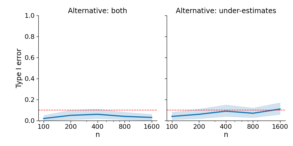
Appendix D Simulation study of Type I error control
The goal of this simulation is to analyze the Type I error of the score-test in finite samples. We test for strong calibration with tolerance . For the original ML algorithm, we train a logistic regression model using 10,000 observations generated with the conditional log odds as
For the audit data, we simulated outcomes where the conditional probabilities were to maximize Type I error. This simulation also reflects situations where ML algorithm is developed for one context and deployed in another, and one is interested in knowing if the ML algorithm is miscalibrated in some subgroup in the new target population.
We perform a one-sided test to determine if the predicted risks are under-estimates and a two-sided test. We implement the CV-based testing procedures for which we have only established asymptotic control of the Type I error rate. We do not include results from the single sample split, since we proved that it provides finite sample control of the Type I error rate. The critical values were set to target a Type I error rate of 0.1. Recall that the one-sided test calculates the critical value by sampling from the single worst-case null distribution, whereas the two-sided test relies on sampling upper bounds of the test statistic. As such, we expect the observed Type I error rate to be lower (i.e. more conservative) for the two-sided test than the one-sided test.
As shown in Figure 4, we observe that Type I error is controlled across a variety of audit dataset sizes, including . So, even though our procedure only guarantees finite sample error rate control for the sample-splitting version, we are able to maintain Type I error control for small sample sizes even in the CV version because the assumptions needed for the CV procedure are very weak.