Chasing
rainbows and ocean glints:
Inner working angle constraints for the Habitable Worlds Observatory
Abstract
NASA is engaged in planning for a Habitable Worlds Observatory (HabWorlds), a coronagraphic space mission to detect rocky planets in habitable zones and establish their habitability. Surface liquid water is central to the definition of planetary habitability. Photometric and polarimetric phase curves of starlight reflected by an exoplanet can reveal ocean glint, rainbows and other phenomena caused by scattering by clouds or atmospheric gas. Direct imaging missions are optimised for planets near quadrature, but HabWorlds’ coronagraph may obscure the phase angles where such optical features are strongest. The range of accessible phase angles for a given exoplanet will depend on the planet’s orbital inclination and/or the coronagraph’s inner working angle (IWA). We use a recently-created catalog relevant to HabWorlds of 164 stars to estimate the number of exo-Earths that could be searched for ocean glint, rainbows, and polarization effects due to Rayleigh scattering. We find that the polarimetric Rayleigh scattering peak is accessible in most of the exo-Earth planetary systems. The rainbow due to water clouds at phase angles of would be accessible with HabWorlds for a planet with an Earth equivalent instellation in systems, while the ocean glint signature at phase angles of would be accessible in systems, assuming an (). Improving the () increases accessibility to rainbows and glints by factors of approximately 2 and 3, respectively. By observing these scattering features, HabWorlds could detect a surface ocean and water cycle, key indicators of habitability.
Keywords:
planets and satellites: terrestrial planets – instrumentation: high angular resolution – planets and satellites: atmospheres1 Introduction
Liquid surface water is closely related to planetary habitability because it is essential for life as we know it. To first order, its presence can be predicted by the flux a planet receives from its star. The habitable zone (HZ) is defined as the range of semi-major axes around a given main sequence star for which a rocky planet may have the right temperature to maintain liquid surface water (Kasting et al. 1993). However, there are many factors besides the incident stellar flux that influence a planet’s ability to hold liquid surface water, such as the atmospheric pressure and geological activity. Detecting liquid surface water on an exoplanet would thus provide important context for the interpretation of possible biosignatures. Variations of the flux and degree of polarisation as an exoplanet orbits its host star—phase variations—could reveal scattering phenomena from condensed water (Bailey 2007, e.g., rainbows;) or specular reflection (i.e., glint) from water oceans (McCullough 2006; Williams & Gaidos 2008, e.g.). However, depending on a planetary system’s architecture, such features can be obscured by the inner working angle () of a telescope’s coronagraph, shown schematically in Fig. 1. In this paper, we quantify the planetary phase angles that would be accessible for direct observations of hypothetical terrestrial planets orbiting in the habitable zones of HabWorlds target stars.
1.1 Angle conventions
As shown in Fig. 1, we define the scattering angle as the planet–star–observer angle (large angles for back-scattering, small angles for forward-scattering) and the supplementary phase angle ( at full phase and at new phase). A planet on a perfectly face-on orbit is always seen at quadrature, , while a planet on an inclined orbit will exhibit a wider range of viewing angles; only perfectly edge-on orbits pass through all possible scattering angles. In some plots, we also report degrees from quadrature, so that both new and full phase are at for edge-on orbits.
1.2 Ocean glint
Ocean glint is the specular (Fresnel) reflection of light off a smooth liquid surface. While glint is a familiar phenomenon on Earth, there is only one other body in the Solar System where it has been observed: the Cassini orbiter captured the glint of sunlight reflecting off the liquid hydrocarbon lakes near Titan’s North Pole as it was observing Titan at crescent phases (Stephan et al. 2010). In the total flux, the glint signal is indeed expected to be most prominent at large planetary phase angles. The maximum degree of polarisation of the glint occurs at the Brewster angle, which is determined by the refractive indices at the interface; between air and liquid water this occurs at a reflection angle of locally on the surface (Zugger et al. 2010; Trees & Stam 2019, at a planetary phase angle of about ; see, e.g.,). This angle therefore varies slightly with the wavelength and the composition of the ocean and the atmosphere. The angular width of the glint in total and polarised flux generally broadens with increasing wave height (Williams & Gaidos 2008; Kopparla et al. 2018; Trees & Stam 2019; Trees & Stam 2022). In general, the glint on a planet will be strongest at red wavelengths because there, Rayleigh scattering and attenuation in the atmosphere are smallest (Robinson et al. 2010; Zugger et al. 2011). This has been observed in Earthshine measurements (Emde et al. 2017; Sterzik et al. 2019; Takahashi et al. 2021). At large phase angles, the forward scattering of light by cloud particles could be confused with glint (Robinson et al. 2010). This confusion can be resolved by measuring polarised phase curves at multiple wavelengths (Trees & Stam 2019), as shown in Fig. 2, or by probing the rainbow, see below. More recently, Ryan & Robinson 2022 have also proposed spectral PCA as a tool to separate glint from atmospheric effects on Earth-like worlds.
Glint provides evidence of specular reflecting surfaces, which, taken in the context of the temperature and types of condensates, may be interpreted as evidence for liquid water. The presence of liquid water on the surface of a planet implies the presence of a water cycle, which provides key context to its habitability and the interpretation of atmospheric biosignatures. Aside from detecting ocean glint, the presence of surface water on Earth-like exoplanets can be established through less direct methods near quadrature such as spectropolarimetry, to infer ocean reflection (Trees & Stam 2022), or through rotational mapping, to identify bright continents and dark oceans (Cowan et al. 2009; Lustig-Yaeger et al. 2019, e.g.,).

1.3 Rainbows, cloudbows, and glories
Rainbows, cloudbows, glories, and other scattering phenomena can dramatically influence the shape of a planet’s photometric and polarimetric phase curves and provide a wealth of information about exoplanets (Karalidi et al. 2012; Stam 2008; Bailey 2007; García Muñoz et al. 2014).11 1 Rainbows occur when light is scattered by rain droplets that are large compared to the wavelength of the light. Cloudbows refer to features occurring at the same phase angles from smaller cloud particles, with the spread in colours invisible to the human eye making them appear white (Bailey 2007, for further discussion, see). In the Solar System, the polarised back-scatter from Titan indicated that the moon’s reflection was due to an atmospheric haze rather than a surface (Zellner 1973), and Venus’s polarised phase curve at three wavelengths showed that its clouds were a H2SO4–water mixture and constrained the droplet size distribution (Hansen & Hovenier 1974). The glory feature in Venus’s flux phase curve was later used to rule out various species as the unknown UV absorber (Petrova 2018). Glories and rainbows are technically visible both in total and polarised flux phase curves in the presence of spherical cloud and/or haze particles, but their strongly polarised nature coupled with the suppression of other polarised features at gibbous and full phases make them more easily characterized with polarimetry than with photometry (Karalidi et al. 2011; Stam 2008; Trees & Stam 2019; Trees & Stam 2022).
The phase angles and wavelength dependence of these features are sensitive to the chemical composition and droplet size distribution of condensates in the atmosphere. As with ocean glint, the detection of liquid condensates on an exoplanet can provide key context to their habitability, potential water cycle, and interpretation of atmospheric biosignatures. In this paper, we define our optimal angle for the detection of a rainbow as that of the peak of the water droplet rainbow at visible wavelengths, which is around a phase angle of (see Fig. 2). Pushing observations to angles closer to the star (smaller and larger phase angles) would allow the determination of the full shape of the rainbow, and enable the identification of rainbows due to the scattering of light by other condensates. The glory can allow further characterization of condensates as its angle and shape also depend on the refractive index, but this glory occurs within a phase angle of , when the on-sky separation is small, as can also be seen in Fig. 2.
1.4 Habitable Worlds Observatory
The National Academy of Sciences Astronomy & Astrophysics 2020 Decadal Survey (National Academies of Sciences, Engineering, and Medicine 2021, hereafter Astro2020) recommended a telescope with the capability to detect signatures of habitability on approximately 25 HZ planets in a new “Great Observatories” program. This requires an instrument with a coronagraph capable of high-contrast imaging and low-resolution spectroscopy at optical to near-infrared wavelengths. The precursor technology recommended by the survey lists “direct imaging to probe polarised ocean glint on terrestrial planets” as a priority capability (National Academies of Sciences, Engineering, and Medicine 2021, Table E.1 in) for ground and space-based observatories. Following the release of this report, NASA recently announced the start of the development of the Habitable Worlds Observatory. The performance and characteristics (e.g., on- or off-axis, diameter, type of segmentation, polarimetry or photometry, coronagraph, ) of HabWorlds will significantly impact the expected exo-Earth yield (Stark et al. 2019) and are still to be determined. They will likely be heavily informed by the LUVOIR (The LUVOIR Team 2019) and HabEx (Gaudi et al. 2020) preparatory studies. For generality, in this work, we report angular separations in milliarcseconds; however, for ease of comparison, Table 1 lists the angular separations corresponding to multiples of for a telescope, as suggested in Astro2020, at representative wavelengths of and .
| mas (at ) | mas (at ) | ||
| IWA | 1 | 20.6 | 34.4 |
| IWA | 2 | 41.3 | 68.8 |
| IWA | 3 | 61.9 | 103.1 |
| IWA | 4 | 82.5 | 137.5 |
| OWA | 32 | 660.0 | 1100.1 |
| OWA | 64 | 1320.1 | 2200.2 |
2 Methods
2.1 Target list
A preliminary target list of nearby stars (maximum distance ) around which HabWorlds may search for habitable rocky planets (assuming a telescope), has been compiled: the NASA Exoplanet Exploration Program’s Mission Star List for the Habitable Worlds Observatory.22 2 Available online: https://exoplanets.nasa.gov/internal_resources/2645_NASA_ExEP_Target_List_HWO_Documentation_2023.pdf This list consists of stars, the majority of which are Sun-like dwarfs: 66 F dwarfs, 55 G dwarfs, 40 K dwarfs, and 3 M dwarfs. The target list is constructed assuming a maximum planet magnitude in the Cousins band of mag and a lower limit of for the planet-star flux ratio. The adopted HZ limits are a semi-major axis of for a solar twin and planet sizes between Earth radii. For non-solar stars, the semi-major axis scales as the square root of the bolometric luminosity normalized to the Sun. This range of orbital separation corresponds to the “conservative habitable zone” (Kasting et al. 1993; Kopparapu et al. 2013). In the remainder of this work, we consider hypothetical Earth-sized planets orbiting at the right distance from their parent star to receive the same flux as the Earth receives from the Sun. By design, all such planets should be observable by HabWorlds at quadrature phase.
2.2 Accessible phase angles
We first define the phase angle ranges over which the various phenomena—glint, Rayleigh scattering peak, rainbow, and glory—manifest themselves in Table 2, also shown in Fig. 2. These ranges are all approximate, as the exact angles where these phenomena dominate depend on the details of the atmospheric and surface properties, as well as on the wavelengths being observed.
| Glory | |||
|---|---|---|---|
| Rainbow | |||
| Rayleigh peak | |||
| Ocean Glint |
A coronagraphic mask can obscure part of a planet’s orbit. As illustrated in Fig. 1, obscuration is a problem at small and large phase angles, when the planet is at small angular separation from its star. The range of accessible phase angles will depend on the of the coronagraph, as well as on the orbital inclination and eccentricity.
2.2.1 Circular, edge-on orbits
The on-sky projected planet distance, (in ) is shown in Fig. 3 for a non-eccentric case with a semi-major axis (in ), at a distance (in ) from the observer. The scattering angle, , is given by
| (1) |
assuming small angles and , where is the on-sky angular separation. We access the minimum/maximum phase angle when reaches the inner working angle separation, thus when . We can rewrite Eq. 1 as:
| (2) |
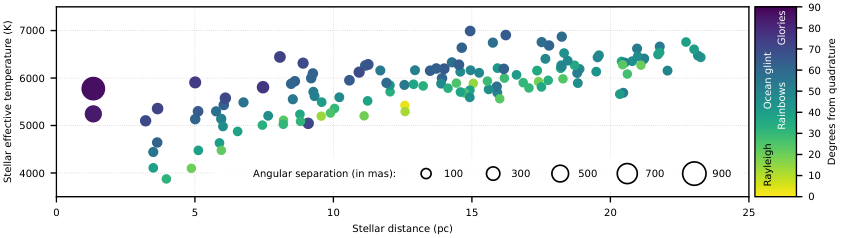
where we define as the difference between the maximum and minimum accessible phase angles. For non-eccentric orbits the maximum and minimum phase angles will be equal sides of quadrature and so represents the maximum angle away from quadrature that can be accessed.
Figure 4 shows for the systems in the HabWorlds target list, assuming an IWA of . As can be seen in Fig. 4, for exoplanets in edge-on circular orbits, it will always be possible to observe the peak polarisation due to Rayleigh scattering, which occurs around quadrature (), while the rainbow angle () will only be accessible for a subset of exoplanets.
2.2.2 Circular, inclined orbits
Most planets are not in edge-on orbits as seen from Earth. For an orbit with an inclination angle (where is face-on), we can identify the following two regimes:
- 1.
The coronagraph does not obscure any part of the sky-projected orbit: the maximum phase angle coverage depends solely on . This holds for orbits that are relatively face-on (small ).
- 2.
The coronagraph does obscure parts of the sky-projected orbit: the phase angle coverage depends only on the and the orbital semi-major axis , following Eq. 2.
The range of accessible phase angles is then
| (3) |
2.3 Monte Carlo simulations of accessible orbits
2.3.1 Circular, randomly inclined orbits
For each of the 164 stars on the HabWorlds target list, we generate random orbits of hypothetical habitable planets with semi-major axes that yield an Earth-equivalent-incident stellar flux. The orbital inclination angles are randomly drawn from a distribution that is uniform in . We then use Eq. 3 to determine the range of accessible phase angles for each hypothetical planet. The solid lines in Fig. 5 show the cumulative distribution of the maximum and minimum accessible phase angles normalised to the total number of systems in the HabWorlds target list for different values of the .
2.3.2 Eccentric, randomly inclined orbits
We repeat the Monte Carlo simulations from Section 2.3.1, assuming the orbital eccentricity follows a beta-distribution with shape parameters and (Kipping 2013). The semi-major axis is kept the same for the circular and eccentric orbits—we do not renormalise the semi-major axis to keep the time-averaged flux the same for all systems. We randomly draw orbits for each star and determine the sky-projected orbits following, for example, Murray & Correia 2010. Orbital eccentricities are drawn from the beta distribution, and inclination angles are uniform in . Figure 6 shows a sample of the generated orbits.
We then calculate the minimum and maximum accessible phase angles for s of . The dashed lines in Fig. 5 show the normalised cumulative distribution of the accessible phase angles for each value of the for eccentric orbits. We also calculate which target planets would be accessible at the phase angles where ocean glint, the rainbow, or the Rayleigh scattering peak occur.
2.4 Simulating contrast curves
A second parameter that is crucial for detecting angular features like rainbows and ocean glint on Earth-like exoplanets is the contrast, that is, the planet-to-star flux ratio. While contrast is not the main focus of this paper, we note that the total and polarised flux contrasts depend on the phase angle, due to a combination of the changing illumination fraction of the observable planetary disk and non-isotropic reflection by the planet. For the contrast calculations, we start with the HabWorlds target list (see Section 2.1), which, for every star, includes an estimated contrast for an Earth-twin in the habitable zone. The contrast is given by (Mahapatra et al. 2023, e.g.,)
| (4) |
where is the planet’s geometric albedo, its radius, is the phase function at phase angle (normalized to at full phase, thus , and is the distance between the planet and its host star.
The contrast estimations in the HabWorlds target list were calculated assuming circular planetary orbits, and Lambertian reflecting planets (Russell 1916) with a geometric albedo equal to 0.2. This albedo value was adopted from the VPL models in Robinson et al. 2011, and the assumption of a Lambert phase function is justifiable given the apparent albedo values derived from Earthshine observations by Qiu et al. 2003 and Pallé et al. 2003. For a more accurate representation of the contrast as a function of the separation, we replace the Lambertian phase function with the models shown in Fig. 2 from Trees & Stam 2019 which assume an Earth-like planet with an ocean surface, a wind-speed of , and patchy liquid water clouds observed at .
We assume that the contrasts in the HabWorlds target list represent the reflected flux at quadrature (), where a Lambertian phase function equals . Using Eq. 4, we correct the contrasts in the HabWorlds target list by dividing them with (= ) and multiplying them by the reflected light fractions of the updated models of Trees & Stam 2019. We then map the orbital phase for circular orbits to the phase angle and on-sky separation, assuming an inclination of . Together, this gives the reflected light contrast as a function of separation for a full orbit. We multiply this flux with the degree of polarisation to obtain the polarised contrast. Figure 7 shows the resulting contrast curves for three of the closest target stars: the M dwarf Lalande 21185, the K dwarf Eri, and the G dwarf Cen A. These calculations are by no means complete or exact, given the many variables that go into the modelling of reflected total and polarised fluxes of Earth-like exoplanets (Trees & Stam 2019; Trees & Stam 2022).

3 Results
3.1 The effect of eccentricity
As shown in Fig. 5, an empirical eccentricity distribution increases the number of systems that can be observed at each phase angle (notably for the red and purple lines). This is because eccentric planets reach orbital separations greater than their semi-major axis, and hence are more likely to “peek out” from behind the coronagraph at extreme orbital phases (albeit with worse contrast due to the greater star-planet separation). The eccentricity does not significantly affect the number of systems for smaller than that used in the selection of the HabWorlds target list (yellow and blue lines).
3.2 Accessible scattering phenomena
Figure 8 and Table 3 show the number of systems in which key scattering phenomena will be accessible for different . The Rayleigh scattering peak in polarization, which can be used to determine if a planet has an atmosphere, appears near quadrature and is therefore accessible in the most systems. The rainbow feature appears further from quadrature (around ), but will still be accessible in a significant fraction of systems. The position and shape of the rainbow peak is sensitive to the properties of the cloud droplets, allowing their characterization if the peak of the rainbow feature can be reached. In most systems, only the first half of the glint feature would be accessible, but this can still be used to identify a liquid ocean on the surface of a planet, a key indicator of habitability.
| Inner Working Angle (IWA) | ||||
| Feature | 21 mas | 41 mas | 62 mas | 83 mas |
| Glory | 0 | 0 | 0 | 0 |
| Ocean Glint | 79 | 43 | 16 | 6 |
| Rainbow | 109 | 90 | 46 | 22 |
| Rayleigh | 154 | 152 | 125 | 78 |
3.3 Contrast curves
The contrast of the planet is also an important factor in assessing the detectability of these scattering phenomena. Figure 7 shows approximate contrast curves for three of the stars in the HabWorlds target list, assuming an Earth-like planet on an edge-on orbit. The overall contrast varies significantly for each system and throughout the orbit. In general, planets orbiting high-mass stars tend to offer larger angular separation but lower contrast ratios. The accessibility of these planets will depend on the starlight suppression of the coronagraph, which is influenced by its . It will be important to consider both the accessible phase angles and contrast limits when deciding on the of the HabWorlds coronagraph if these scattering features are to be observed.
4 Discussion
In this work, we consider each orbit to have a semi-major axis for which it would receive the same flux as Earth assuming a circular orbit. As Earth is at the inner edge of the Habitable Zone, our estimates for the number of systems with accessible scattering features is conservative. However, as we are only considering the accessibility of scattering features, it is possible to scale the results presented here for different semi-major axes. This is because the range of accessible features is determined only by the amount of the orbit covered by the mask, therefore increasing the semi-major axis of an orbit (e.g., double) is equivalent to decreasing the apparent mask size by the same factor (e.g., half).
5 Conclusions
The Habitable Worlds Observatory is a coronagraphic space telescope envisioned to detect and characterize Earth-like exoplanets in the 2040s. The instrument design and capabilities are still under development and should be driven by the mission’s science goals. In this work, we investigated the possibility of using HabWorlds to detect optical phenomena with specific angular features in polarised and unpolarised reflected light, such as rainbows, ocean glint, and glories, which could establish a planet’s habitability. We primarily focused on the range of accessible phase angles given the limitations of the coronagraphic and aimed to investigate which phenomena could potentially be observed. While we do not consider the detectability of the scattering features beyond their accessibility, we show they are typically more distinct in polarised light, but the exoplanet-star contrast ratio is lower than the unpolarised light contrast ratio.
The desire to detect and characterize a large number of Earth-like exoplanets, and the intrinsic occurrence of such planets around different stellar spectral types, will drive the choice of coronagraphic for HabWorlds. Assuming a , of planetary systems in the NASA Exoplanet Exploration Program’s Mission Star List for HabWorlds would be accessible at phases angles with maximal polarisation from Rayleigh scattering. The rainbow of light that is scattered in droplets of water clouds and ocean glint, both of which indicate the presence of a water cycle which provides additional context to the habitability of an exoplanet, would be accessible in and of systems respectively. The presence of a water cycle on Earth-like exoplanets in the remaining systems would have to be established through less direct methods: spectropolarimetry or rotational mapping. To observe more scattering features in more systems, HabWorlds would need a smaller by use of a better-controlled coronagraph and potentially a larger primary mirror.
Data Availability
The NASA ExEP target list containing the data used for our simulations is available online.33 3 https://exoplanets.nasa.gov/exep/science-overview/ This paper has been prepared using the showyourwork! framework (Luger et al. 2021), which makes the entire Python code to create all figures and the associated data available in an online repository to facilitate the reproducibility of our work.44 4 https://github.com/mkenworthy/HWObows/
Acknowledgements
The 2023 Optimal Exoplanet Imagers workshop, which sparked the work presented in this manuscript, was made possible thanks to the logistical and financial support of the Lorentz Center, Leiden, The Netherlands. The research presented in this paper was initiated at a workshop held in Leiden in February 2023 and was partially supported by NOVA (the Netherlands Research School for Astronomy) and by the European Research Council (ERC) under the European Union’s Horizon 2020 research and innovation programme (grant agreement № 866001—EXACT).
SRV and JLB acknowledge funding from the European Research Council (ERC) under the European Union’s Horizon 2020 research and innovation program under grant agreement № 805445. TDG acknowledges funding from the Max Planck ETH Center for Learning Systems. SLC acknowledges support from an STFC Ernest Rutherford Fellowship. KB acknowledges support from NASA Habitable Worlds grant № 80NSSC20K152, and previous support for related work from NASA Astrobiology Institute’s Virtual Planetary Laboratory under Cooperative Agreement № NNA13AA93A. IL acknowledges the support by a postdoctoral grant issued by the Centre National d’Études Spatiales (CNES) in France. PB, IL, and YG were supported by the Action Spécifique Haute Résolution Angulaire (ASHRA) of CNRS/INSU co-funded by CNES. EHP is supported by the NASA Hubble Fellowship grant #HST-HF2-51467.001-A awarded by the Space Telescope Science Institute, which is operated by the Association of Universities for Research in Astronomy, Incorporated, under NASA contract NAS5-26555. LA and EC acknowledge funding from the European Research Council (ERC) under the European Union’s Horizon Europe research and innovation programme (ESCAPE, grant agreement № 101044152). OA and LK acknowledge funding from the European Research Council (ERC) under the European Union’s Horizon 2020 research and innovation programme (grant agreement № 819155). SYH was funded by the generous support of the Heising-Simons Foundation. RJP is supported by NASA under award number 80GSFC21M0002. OHS acknowledges funding from the Direction Scientifique Générale de l’ONERA (ARE Alioth).
This work has made use of numpy (Harris et al. 2020), scipy (Virtanen et al. 2020), matplotlib (Hunter 2007), and astropy55 5 https://www.astropy.org, a community-developed core Python package and an ecosystem of tools and resources for astronomy (Astropy Collaboration et al. 2013; Astropy Collaboration et al. 2018; Astropy Collaboration et al. 2022). The colourblind-friendly colour schemes used in this paper were taken from Petroff 2021. This research has made use of NASA’s Astrophysics Data System Bibliographic Services and the SIMBAD database, operated at CDS, Strasbourg, France.
References
- Astropy Collaboration et al. (2013) Astropy Collaboration et al., 2013, A&A, 558, A33
- Astropy Collaboration et al. (2018) Astropy Collaboration et al., 2018, AJ, 156, 123
- Astropy Collaboration et al. (2022) Astropy Collaboration et al., 2022, ApJ, 935, 167
- Bailey (2007) Bailey J., 2007, Astrobiology, 7, 320
- Cowan et al. (2009) Cowan N. B., et al., 2009, ApJ, 700, 915
- Cox & Munk (1954) Cox C., Munk W., 1954, Journal of the Optical Society of America, 44, 838
- Emde et al. (2017) Emde C., Buras-Schnell R., Sterzik M., Bagnulo S., 2017, A&A, 605, A2
- García Muñoz et al. (2014) García Muñoz A., Pérez-Hoyos S., Sánchez-Lavega A., 2014, A&A, 566, L1
- Gaudi et al. (2020) Gaudi B. S., et al., 2020, arXiv e-prints, p. arXiv:2001.06683
- Hansen & Hovenier (1974) Hansen J. E., Hovenier J. W., 1974, Journal of the Atmospheric Sciences, 31, 1137
- Harris et al. (2020) Harris C. R., et al., 2020, Nature, 585, 357
- Hunter (2007) Hunter J. D., 2007, Computing in Science & Engineering, 9, 90
- Karalidi et al. (2011) Karalidi T., Stam D. M., Hovenier J. W., 2011, A&A, 530, A69
- Karalidi et al. (2012) Karalidi T., Stam D. M., Hovenier J. W., 2012, A&A, 548, A90
- Kasting et al. (1993) Kasting J. F., Whitmire D. P., Reynolds R. T., 1993, Icarus, 101, 108
- Kipping (2013) Kipping D. M., 2013, MNRAS, 434, L51
- Kopparapu et al. (2013) Kopparapu R. K., et al., 2013, ApJ, 765, 131
- Kopparla et al. (2018) Kopparla P., Natraj V., Crisp D., Bott K., Swain M. R., Yung Y. L., 2018, AJ, 156, 143
- Luger et al. (2021) Luger R., Bedell M., Foreman-Mackey D., Crossfield I. J. M., Zhao L. L., Hogg D. W., 2021, arXiv e-prints, p. arXiv:2110.06271
- Lustig-Yaeger et al. (2019) Lustig-Yaeger J., Meadows V. S., Lincowski A. P., 2019, AJ, 158, 27
- Mahapatra et al. (2023) Mahapatra G., Abiad F., Rossi L., Stam D. M., 2023, A&A, 671, A165
- McCullough (2006) McCullough P. R., 2006, arXiv e-prints, pp astro–ph/0610518
- Murray & Correia (2010) Murray C. D., Correia A. C. M., 2010, in Seager S., ed., , Exoplanets. University of Arizona Press, Tucson, AZ, pp 15–23, doi:10.48550/arXiv.1009.1738
- National Academies of Sciences, Engineering, and Medicine (2021) National Academies of Sciences, Engineering, and Medicine 2021, Pathways to Discovery in Astronomy and Astrophysics for the 2020s. The National Academies Press, Washington, DC, doi:10.17226/26141
- Pallé et al. (2003) Pallé E., et al., 2003, Journal of Geophysical Research (Atmospheres), 108, 4710
- Petroff (2021) Petroff M. A., 2021, arXiv e-prints, p. arXiv:2107.02270
- Petrova (2018) Petrova E. V., 2018, Icarus, 306, 163
- Qiu et al. (2003) Qiu J., et al., 2003, Journal of Geophysical Research (Atmospheres), 108, 4709
- Robinson et al. (2010) Robinson T. D., Meadows V. S., Crisp D., 2010, ApJ, 721, L67
- Robinson et al. (2011) Robinson T. D., et al., 2011, Astrobiology, 11, 393
- Russell (1916) Russell H. N., 1916, ApJ, 43, 173
- Ryan & Robinson (2022) Ryan D. J., Robinson T. D., 2022, Planetary Sciences Journal, 3, 33
- Stam (2008) Stam D. M., 2008, A&A, 482, 989
- Stark et al. (2019) Stark C. C., et al., 2019, Journal of Astronomical Telescopes, Instruments, and Systems, 5, 024009
- Stephan et al. (2010) Stephan K., et al., 2010, Geophys. Res. Lett., 37, L07104
- Sterzik et al. (2019) Sterzik M. F., Bagnulo S., Stam D. M., Emde C., Manev M., 2019, A&A, 622, A41
- Takahashi et al. (2021) Takahashi J., Itoh Y., Matsuo T., Oasa Y., Bach Y. P., Ishiguro M., 2021, A&A, 653, A99
- The LUVOIR Team (2019) The LUVOIR Team 2019, arXiv e-prints, p. arXiv:1912.06219
- Trees & Stam (2019) Trees V. J. H., Stam D. M., 2019, A&A, 626, A129
- Trees & Stam (2022) Trees V. J. H., Stam D. M., 2022, A&A, 664, A172
- Virtanen et al. (2020) Virtanen P., et al., 2020, Nature Methods, 17, 261
- Williams & Gaidos (2008) Williams D. M., Gaidos E., 2008, Icarus, 195, 927
- Zakovryashin & Prigarin (2020) Zakovryashin A. V., Prigarin S. M., 2020, Russian Journal of Numerical Analysis and Mathematical Modelling, 35, 367
- Zellner (1973) Zellner B., 1973, Icarus, 18, 661
- Zugger et al. (2010) Zugger M. E., Kasting J. F., Williams D. M., Kane T. J., Philbrick C. R., 2010, ApJ, 723, 1168
- Zugger et al. (2011) Zugger M. E., Kasting J. F., Williams D. M., Kane T. J., Philbrick C. R., 2011, ApJ, 739, 12
Author affiliations
1Astrophysics, Department of Physics, University of Oxford, Denys Wilkinson Building, Keble Road, Oxford OX1 3RH, UK
2Max Planck Institute for Intelligent Systems, Max-Planck-Ring 4, 72076 Tübingen, Germany
3ETH Zurich, Institute for Particle Physics & Astrophysics, Wolfgang-Pauli-Str. 27, 8092 Zurich, Switzerland
4Department of Earth and Planetary Sciences, University of California, Riverside, CA 92521, USA
5NASA Nexus for Exoplanet System Science, Virtual Planetary Laboratory Team, Seattle, WA 98195, USA
6NASA Nexus for Exoplanet System Science, Terrestrial Polarization Team, Orlando, FL 32826, USA
7Centre for Exoplanet Research, School of Physics and Astronomy, University of Leicester, University Road, Leicester, LE1 7RH, UK
8Department of Earth & Planetary Sciences and Department of Physics, McGill University, 3600 rue University, Montréal, QC, H3A 2T8, Canada
9Leiden Observatory, Leiden University, P.O. Box 9513, 2300 RA Leiden, The Netherlands
10SRON Netherlands Institute for Space Research, Niels Bohrweg 4, 2333 CA, Leiden, The Netherlands
11LESIA, Observatoire de Paris, Université PSL, CNRS, Sorbonne Université, Université de Paris, 92195 Meudon, France
12Department of Physics, University of California, Santa Barbara, CA 93106, USA
13Department of Geoscience & Remote Sensing, Delft University of Technology, Stevinweg 1, 2628 CN, Delft, The Netherlands
14Royal Netherlands Meteorological Institute (KNMI), Utrechtseweg 297, 3731 GA, de Bilt, The Netherlands
15Delft University of Technology, Kluyverweg 1, 2629 HS Delft, The Netherlands
16STAR Institute, Université de Liège, Allée du six Août 19c, 4000 Liège, Belgium
17Aix Marseille Université, CNRS, CNES, LAM, Marseille, France
18NASA Ames Research Center, Bldg. 245, Moffett Field, USA
19Université Grenoble Alpes, CNRS, IPAG, 38000 Grenoble, France
20Department of Astronomy, California Institute of Technology, Pasadena, CA, 91125, USA
21Department of Astronomy & Astrophysics, University of California, Santa Cruz, CA 95064, USA
22Steward Observatory, University of Arizona, 933 North Cherry Avenue, Tucson, AZ 85719, USA
23DTIS, ONERA, Université Paris Saclay, 91123 Palaiseau, France
24DOTA, ONERA, 92322 Châtillon, France
25Subaru Telescope, NAOJ, USA
26College of Optical Sciences, University of Arizona, Tucson, AZ 87521, USA
27Astrobiology Center, 2 Chome-21-1, Osawa, Mitaka, Tokyo, 181-8588, Japan
28NASA Goddard Space Flight Center, 8800 Greenbelt Rd, Greenbelt, MD 20771, USA
29University of Maryland Baltimore County, 1000 Hilltop Cir, Baltimore, MD 21250, USA
30Faculty of Aerospace Engineering, TU Delft, Building 62, Kluyverweg 1, 2629 HS Delft, The Netherlands
31National Research Council Canada, Herzberg Astronomy and Astrophysics Research Center, Victoria, B.C., Canada
32European Space Agency, ESTEC, Keplerlaan 1, 2200 AG Noordwijk, The Netherlands
33Université Côte d’Azur, Observatoire de la Côte d’Azur, CNRS, Laboratoire Lagrange, France
34Space Telescope Science Institute, 3700 San Martin Drive, Baltimore, MD 21218, USA