Generative convective parametrization of dry atmospheric boundary layer

We consider the Boussinesq limit of the Navier–Stokes equations which is given by

	$\displaystyle\frac{\partial{\bf v}}{\partial t}+{\bf\nabla}\cdot({\bf v}\otimes{\bf v})$	$\displaystyle=-{\bf\nabla}\pi+\nu{\bf\nabla}^{2}{\bf v}+b{\bf e}_{z}\,,$		(10)
	$\displaystyle{\bf\nabla}\cdot{\bf v}$	$\displaystyle=0\,,$		(11)
	$\displaystyle\frac{\partial b}{\partial t}+{\bf\nabla}\cdot({\bf v}b)$	$\displaystyle=\kappa{\bf\nabla}^{2}b\,,$		(12)

where $\pi$ is a modified dynamic pressure or kinematic pressure, i.e., a deviation from the pressure in the hydrostatic balance divided by a reference density. Quantity $\nu$ is the kinematic viscosity, $\kappa$ is the buoyancy diffusivity.

The velocity field ${\bf v}({\bf x},t)=(u,v,w)$ satisfies no-slip boundary conditions at the bottom and free-slip boundary conditions at the top Garcia and Mellado 2014. The buoyancy field $b({\bf x},t)$ satisfies Neumann boundary conditions at the bottom and the top. The surface buoyancy flux is given by $B_{0}$. Periodic boundary conditions are imposed in the horizontal directions for all fields. The initial condition is ${\bf v}=0$ and, for the buoyancy,

$$b_{\rm bg}(z)=N_{0}^{2}z+f(z)\,,$$

(13)

where $f(z)$ is the variation near the bottom surface to satisfy $-\kappa\partial b/\partial z=B_{0}$. The function $f(z)$ is only non-zero very near the surface and we consider long enough times for the effects of $f(z)$ on the results to be negligibly small. The quantity $N_{0}$ is the Brunt-Väisälä frequency in (13). The Prandtl number $Pr$ and the buoyancy Reynolds number are the two central dimensionless parameters in this setup. They are given by

$$Pr=\frac{\nu}{\kappa}\,,\quad\quad Re_{0}=\frac{B_{0}}{\nu N_{0}^{2}}\,.$$

(14)

Times are expressed in units of $N_{0}^{-1}$ and lengths in units of the Ozmidov-type scale which is given by

$$L_{0}=\left(\frac{B_{0}}{N_{0}^{3}}\right)^{1/2}\,.$$

(15)

The Prandtl number is $Pr=1$ in the present DNS.

In the convective boundary layer, there is no upper lid that confines the motion; a turbulent boundary layer forms next to the bottom surface. The difference to standard Rayleigh-Bénard convection is that here the boundary layer is only caused by turbulent free convection, forced by a constant heat flux at the bottom surface. The convective boundary layer (CBL) warms and thickens with respect to time. The top boundary of the computational domain is placed far enough to not influence the boundary-layer properties, and otherwise the height of the computational domain becomes unimportant for the analysis.

Except for the CBL, the density in the region above the boundary layer is stably stratified, which hinders the growth of the boundary layer. This region above the boundary layer is referred to as free troposphere or free atmosphere; it is equivalent to the free-stream in a shear-driven boundary layer. One effect of this stratification is that the transition region from the turbulent boundary layer to the non-turbulent free stream is thinner than in the case without stratification. This is because the stratification of the free troposphere hinders the vertical displacement of fluid particles. This transition region is referred to as the entrainment zone. Another effect is that this stratification hinders the growth of the CBL thickness, to the point that the characteristic time for changes of mean properties is small compared to the large eddy turnover time, and a statistically quasi-steady state is observed.

This stratification of the free-stream region is imposed by setting the initial condition of the buoyancy field as $b_{\mathrm{bg}}=N_{0}^{2}z$, see (13). The transition region between the turbulent boundary layer and the free tropopause (i.e., the entrainment zone) occurs where the mean profile of buoyancy, $\langle b(z)\rangle$, changes from the vertically constant value inside the turbulent CBL to the linear profile $b_{\mathrm{bg}}=N_{0}^{2}z$ in the non-turbulent free troposphere, see also Fig. 1(G) in the main text. We refer to the vertical location of this thin transition region as CBL top. There are various ways to define the CBL top and thus the thickness of the whole convective boundary layer. To a first approximation, they all are proportional to the encroachment height which is defined as Carson and Smith 1975; Garcia and Mellado 2014

$$h(t)=\left\{2N_{0}^{-2}\int_{0}^{z_{\infty}}(\langle b(z)\rangle_{x,y}-b_{\mathrm{bg}}(z))\mathrm{d}z\right\}^{1/2}\,.$$

(16)

From the point of view of dimensional analysis, we have substituted the cell height in a Rayleigh-Bénard setup by $L_{0}$ which was defined in (15). It characterizes the thickness of the transition region at the top of the CBL. The reference length $L_{0}$ is constant, but $h$ increases with time $t$. Consider the mean buoyancy equation with statistical homogeneity in the horizontal directions. Then follows from (12)

$$\frac{\partial}{\partial t}[\langle b\rangle_{x,y}-b_{\rm bg}(z)]=-\frac{\partial}{\partial z}\left[\langle w^{\prime}b^{\prime}\rangle_{x,y}-\kappa\frac{\partial\langle b\rangle_{x.y}}{\partial z}\right]\,,$$

(17)

where we have added the time-independent profile $b_{\rm bg}(z)$ on the left hand side. Integrate (17) from $z=0$ to $z=z_{\infty}$ and use the fact that far away from the surface $\langle b\rangle_{x,y}\to b_{\rm bg}(z)=N_{0}^{2}z$. This results to

$$\frac{\partial}{\partial t}\int_{0}^{z_{\infty}}[\langle b\rangle_{x,y}-b_{\rm bg}(z)]dz=\kappa N_{0}^{2}+B_{0}=B_{0}\left(1+\frac{1}{PrRe_{0}}\right)\,.$$

(18)

Thus an additional integration with respect to time, together with (16), gives

$$\int_{0}^{z_{\infty}}[\langle b\rangle_{x,y}-b_{\rm bg}(z)]dz=B_{0}\left(1+\frac{1}{PrRe_{0}}\right)(t-t_{0})=\frac{h^{2}N_{0}^{2}}{2}\,.$$

(19)

Encroachment height and Ozmidov-type scale, see (15), are then related according to

$$\frac{h(t)}{L_{0}}=\left[2N_{0}(t-t_{0})\left(1+\frac{1}{PrRe_{0}}\right)\right]^{1/2}\;,$$

(20)

where $t_{0}$ is an integration constant. See also (12) in the main text for $Pr=1$. The growth rate of $h(t)$ is referred to as mean entrainment velocity

$$w_{\mathrm{e}}\equiv\frac{\mathrm{dh}}{\mathrm{d}t}\,.$$

(21)

The convective Rayleigh number, which is given by

$$Ra_{c}(t)=\frac{B_{0}h(t)^{4}}{\nu\kappa^{2}}\,,$$

(22)

increases as $h(t)$ increases with time $t$.

Discretization in space is performed using sixth-order spectral-like compact finite differences on a structured Cartesian grid Mellado and Ansorge 2012. A low-storage fourth-order accurate Runge–Kutta scheme is used for time stepping. The discrete solenoidal constraint is satisfied to machine accuracy using a Fourier decomposition along the periodic horizontal planes in $x$-$y$ directions and a factorization of the resulting set of equations along the vertical coordinate $z$. The local ratio between the vertical grid spacing, $\Delta z$, and the Kolmogorov scale, $\eta_{K}$, is $\Delta z/\eta_{K}\lesssim 1.2$.

In the present proof-of-concept study we omit phase changes and cloud formation. The liquid-water potential temperature $\theta_{l}$ reduces then to the virtual potential temperature $\theta$ and the buoyancy $b$ becomes

$$b({\bf x},t)=g\frac{\theta_{\rm v}({\bf x},t)-\theta_{{\rm v},0}}{\theta_{{\rm v},0}}\,,$$

(23)

with the acceleration due to gravity $g$ and the virtual potential temperature at the surface $\theta_{{\rm v},0}$. The eddy diffusivity mass-flux closure for the sub-grid scale buoyancy flux is given by Siebesma and Holtslag 1996; Siebesma et al. 2007; Witte et al. 2022,

$$\rho_{0}\langle w^{\prime}b^{\prime}(z)\rangle_{x,y}=-\rho_{0}\kappa_{t}\frac{\partial\langle b\rangle_{x,y}}{\partial z}+M_{u}(\langle b(z)\rangle_{u}-\langle b(z)\rangle_{x,y})\,.$$

(24)

Here, $\rho_{0}$ is the constant reference density in the lower atmospheric boundary layer and $M_{u}$ is the unknown mass flux. As already said in the main text, the horizontal cross section $A$ can be decomposed into disjoint updraft regions (u) and the remaining environment (e), i.e., $A_{\rm total}=A_{u}\cup A_{e}$. For simplicity we will denote $A_{\rm total}$ simply by $A$ to ease notation. The first term in (24) is the standard Boussinesq term for a turbulent stress which contains the eddy diffusivity $\kappa_{t}$ and the mean buoyancy gradient. The additional second term comprises the mass-flux parametrization. In detail,

	$\displaystyle\langle w^{\prime}b^{\prime}(z)\rangle_{x,y}$	$\displaystyle=\frac{1}{A}\int_{A}(w-\langle w\rangle_{x,y})(b-\langle b\rangle_{x,y})\,dA\,,$		(25)
	$\displaystyle a_{u}\langle w^{\prime}b^{\prime}(z)\rangle_{u}$	$\displaystyle=\frac{1}{A}\int_{A}(w-\langle w\rangle_{u})(b-\langle b\rangle_{u})\,dA\,,$		(26)
	$\displaystyle(1-a_{u})\langle w^{\prime}b^{\prime}(z)\rangle_{e}$	$\displaystyle=\frac{1}{A}\int_{A}(w-\langle w\rangle_{e})(b-\langle b\rangle_{e})\,dA\,,$		(27)

with the area fractions $a_{u}=A_{u}/A$ and $1-a_{u}=A_{e}/A$. We neglect the first gradient term on the right hand side of (24) for a while. The second term of (24) can be rewritten to

$$\langle w^{\prime}b^{\prime}\rangle_{x,y}=a_{u}\langle w^{\prime}b^{\prime}\rangle_{u}+(1-a_{u})\langle w^{\prime}b^{\prime}\rangle_{e}+a_{u}(1-a_{u})[\langle w\rangle_{u}-\langle w\rangle_{e}][\langle b\rangle_{u}-\langle b\rangle_{e}]\,.$$

(28)

The first term quantified the buoyancy flux connected with $A_{u}$, the second the one with $A_{e}$, and the third is an exchange term due to organized turbulence which connects both. The following approximations can be made: (i) $a_{u}\ll 1$, in practice mostly about 5 %; (ii) $\langle w\rangle_{e}\simeq\langle w\rangle_{x,y}$, and (iii) $\langle b\rangle_{e}\simeq\langle b\rangle_{x,y}$. This results to the mass-flux parametrization

$$\langle w^{\prime}b^{\prime}(z)\rangle_{x,y}\simeq\frac{M_{u}}{\rho_{0}}(\langle b(z)\rangle_{u}-\langle b(z)\rangle_{x,y})\quad\mbox{with}\quad M_{u}=\rho_{0}a_{u}[\langle w(z)\rangle_{u}-\langle w(z)\rangle_{x,y}]\,,$$

(29)

with the undetermined mass flux $M_{u}$. Recall also that the mass flux carries the physical dimension of kg m^-2s^-1. A plume model is required to determine this unknown quantity which is discussed in the following.

(12) of the present model is the counterpart of the set of prognostic equations in a global circulation model. We apply a Reynolds decomposition and obtain the following unclosed coarse-grid equation Siebesma and Cuijpers 1995

$$\frac{\partial\langle b(z)\rangle_{x,y}}{\partial t}=-\frac{1}{\rho_{0}}\frac{\partial}{\partial z}[\rho_{0}\langle w^{\prime}b^{\prime}(z)\rangle_{x,y}]+\frac{\partial\langle b(z)\rangle_{x,y}}{\partial t}\Bigg|_{\rm forcing}\,.$$

(30)

All remaining terms due to horizontal mean advection and diffusion are summarized in the last term of (30) as a forcing term. Note that we get in this way an effective vertical transport model without any information on the spatial horizontal mesoscale organisation of the convective turbulence which the DNS in the main text display. The area decomposition into $A_{u}$ and $A_{e}$ gives

$$\langle b(z)\rangle_{x,y}=a_{u}\langle b(z)\rangle_{u}+(1-a_{u})\langle b(z)\rangle_{e}\,.$$

(31)

Equations (28) and (31) are now plugged into (30). We use that $a_{u}(1-a_{u})\approx a_{u}$ since $a_{u}\ll 1$ and apply additionally the approximations (ii) and (iii) from the last subsection. This leads to the following updraft budget equation (omitting the $z$ argument),

$\displaystyle\rho_{0}\frac{\partial}{\partial t}[a_{u}\langle b\rangle_{u}]=-\frac{\partial}{\partial z}[\rho_{0}a_{u}\langle w^{\prime}b^{\prime}\rangle_{u}]-\frac{\partial}{\partial z}[\underbrace{\rho_{0}a_{u}(\langle w\rangle_{u}-\langle w\rangle_{x,y})}_{=M_{u}}\langle b\rangle_{u}]+E\langle b\rangle_{e}-D\langle b\rangle_{u}+\rho_{0}a_{u}\frac{\partial\langle b\rangle_{x,y}}{\partial t}\Bigg|_{\rm forcing}\,,$

(32)

and the corresponding downdraft budget equation

$\displaystyle\rho_{0}\frac{\partial}{\partial t}[(1-a_{u})\langle b\rangle_{e}]=-\frac{\partial}{\partial z}[\rho_{0}(1-a_{u})\langle w^{\prime}b^{\prime}\rangle_{e}]+\frac{\partial}{\partial z}[M_{u}\langle b\rangle_{e}]-E\langle b\rangle_{e}+D\langle b\rangle_{u}+\rho_{0}(1-a_{u})\frac{\partial\langle b\rangle_{x,y}}{\partial t}\Bigg|_{\rm forcing}\,.$

(33)

We have added two terms in both equations to express the mass exchange due to entrainment and detrainment with rates $E$ and $D$, respectively. Adding both equations brings us back to (30). Furthermore, a continuity equation is required which can be obtained from one of the budget equations by substituting $\langle b\rangle$ with 1. This gives

$$\rho_{0}\frac{\partial a_{u}}{\partial t}=-\frac{\partial M_{u}}{\partial z}+E-D\,.$$

(34)

Next a (statistically) steady state is assumed such that (32) and (34) simplify to, see also ref. Siebesma et al. 2007,

	$\displaystyle\frac{\partial}{\partial z}[M_{u}\langle b\rangle_{u}]$	$\displaystyle=-\frac{\partial}{\partial z}[\rho_{0}a_{u}\langle w^{\prime}b^{\prime}\rangle_{u}]+M_{u}\epsilon\langle b\rangle_{e}-M_{u}\delta\langle b\rangle_{u}\,,$		(35)
	$\displaystyle\frac{\partial M_{u}}{\partial z}$	$\displaystyle=M_{u}(\epsilon-\delta)\,,$		(36)

where fractional entrainment and detrainment rates follow from $E=M_{u}\epsilon$ and $D=M_{u}\delta$, respectively. When the first term on the right hand side of (35) is set to zero, both equations can be combined to give the following simple updraft equation

$$\frac{\partial\langle b\rangle_{u}}{\partial z}=\epsilon(\langle b\rangle_{x,y}-\langle b\rangle_{u})\,.$$

(37)

Furthermore, we need an equation for $\langle w\rangle_{u}$ such that we can close the buoyancy flux model Schumann and Moeng 1991; Siebesma et al. 2007. This is obtained from the momentum balance for the updrafts, assuming again a steady regime. This gives

$$-\frac{1}{2}\frac{\partial\langle w\rangle_{u}^{2}}{\partial z}-C_{1}\epsilon\langle w\rangle_{u}^{2}-\frac{1}{\rho_{0}}\frac{\partial\langle p\rangle_{x,y}}{\partial z}+\langle b\rangle_{u}-\langle b\rangle_{x,y}=0\,.$$

(38)

This equation went again through a number of simplification steps: (i) the first term results from the nonlinear advection of $\langle w\rangle_{u}$, (ii) the second term encloses all remaining advection terms, (iii) the effective entrainment rate which is connected with the turbulent mixing in (ii) is assumed to be directly proportional to the entrainment for $\langle b\rangle_{u}$ in (37). (iv) The pressure gradient term is approximated finally to be $\partial(\mu\langle w\rangle_{u})/\partial z$. This is the last step and the mass-flux parametrization comprises the following coupled system of equations which would have to be solved together with the mean prognostic equation for $\langle b\rangle_{x,y}$,

	$\displaystyle\frac{\partial\langle b\rangle_{u}}{\partial z}$	$\displaystyle=\epsilon(\langle b\rangle_{x,y}-\langle b\rangle_{u})\,,$		(39)
	$\displaystyle\frac{1}{2}(1-2\mu)\frac{\partial\langle w\rangle_{u}^{2}}{\partial z}+C_{1}\epsilon\langle w\rangle_{u}^{2}$	$\displaystyle=\langle b\rangle_{u}-\langle b\rangle_{x,y}\,.$		(40)

If we know $\langle w\rangle_{u}$ and $\langle b\rangle_{u}$ then we can calculate the second term on the right hand side of the EDMF model in (24) for a given $a_{u}$. The model parameters $\epsilon$, $C_{1}$, and $\mu$ are however unknown. Large eddy simulations studies by Siebesma et al. Siebesma et al. 2007 suggest $C_{1}\simeq 0.5$ and $\mu\simeq 0.15$. The fractional entrainment rate $\epsilon$, which will be height dependent, is more recently included as a stochastic multi-plume model, i.e., for each plume $i$ the EDMF model equations are solved. The entrainment rates $\epsilon_{i}$ are chosen from a Poisson distribution Witte et al. 2022.

The eddy-diffusivity $\kappa_{t}$ is implemented by a simple profile method Holtslag and Duynkerke 1998 and results to

$\displaystyle\kappa_{t}(z)=k\left(39k\frac{z}{h}\right)^{1/3}\frac{z}{h}\left(1-\frac{z}{h}\right)^{2}w_{\ast}h\,,$

(41)

where $k\approx 0.4$ is the von Kármán constant. The mass-flux contributions were obtained by integrating equations (39) and (40) using a fourth-order Runge-Kutta scheme. We choose the starting height $z_{0}>0$ together with the boundary conditions

	$\displaystyle\langle b(z_{0})\rangle_{u}$	$\displaystyle=\langle b(z_{0})\rangle+\alpha B_{0}/\sigma_{w},$		(42)
	$\displaystyle\langle w(z_{0})\rangle_{u}^{2}$	$\displaystyle=\sigma_{w}^{2}(z_{0}),$		(43)

where we make use of an empirical standard deviation $\sigma_{w}$ as in ref. Holtslag and Moeng 1991 which is given by

$\displaystyle\sigma_{w}(z)\simeq 1.3\left(0.6\frac{z}{h}\right)^{1/3}\left(1-\frac{z}{h}\right)^{1/2}w_{\ast},$

(44)

which fits well for the present direct numerical simulations as seen in Fig. 7.

Furthermore, we use an entrainment rate profile as suggested in van Ulden 1997; Siebesma et al. 2007 which is given by

$\displaystyle\epsilon\simeq 0.4\left(\frac{1}{z}+\frac{1}{h-z}\right).$

(45)

These input lead to the profiles in Fig. 5 of the main text which we used to compare this closure with our machine learning results.

A Generative Adversarial Network (GAN) Goodfellow et al. 2014 is a neural network comprising two interconnected and adversarial components: a generator and a discriminator (or critic). The generator generates synthetic data, in our case, horizontal slices of an atmospheric boundary layer simulation. The discriminator’s role is to distinguish between the synthetic data produced by the generator and real data from the DNS. The two components are trained simultaneously in a competitive manner, with the generator striving to generate data that can fool the critic and the critic continuously improving its ability to classify the data correctly. This adversarial relationship drives the GAN to produce increasingly realistic, high-quality synthetic data. The training of the network is completed once the Nash equilibrium is reached Nash 1950; the discriminator is unable to distinguish synthetically generated and ground truth data. Then the generator can be decoupled from the discriminator and operate autonomously.

Specifically, we use the Wasserstein–GAN (WGAN) formulation from Arjovsky et al. Arjovsky et al. 2017, which solves the vanishing gradient problem of the generator of the original GAN model. This is done using the Wasserstein distance (or Earth-movers distance) between the synthetic and real data in the WGAN loss function. In this way, the generator network will overcome the initial phase, where the discriminator will quickly identify the generated data samples and the GAN training ends in favor of the critic network. Furthermore, the WGAN shows greater stability and convergence during the training.

Here, we use a generator with a U-shaped deep neural network structure, in short U-Net Ronneberger et al. 2015; Fonda et al. 2019. It has seven contraction and seven subsequent expansion layers. After each contraction layer, the spatial dimensions are halved via a convolution operation, while the channel dimensions are doubled. The opposite is done in the expansion path via transposed convolutions. Both paths are connected via residual connections, allowing for a direct information flow between two layers in the contraction and expansion paths of the U-shape. The activation function was chosen as the Parametric Rectified Linear Unit He et al. 2015 (PReLU)

$\displaystyle{\rm PReLU}(x)=\left\{\begin{array}[]{lr}x,&\text{if }x\geq 0\\ ax,&{\rm otherwise}\end{array}\right.$

where the slope $a$ is a learnable parameter. The discriminator network consists of eight convolution layers, which reduce the input data to a scalar score. Here, the PReLU activation was used as well. Finally, to increase the variance of the network, we use Dropout layers, which set the layer output to zero with a probability of $0.3$.

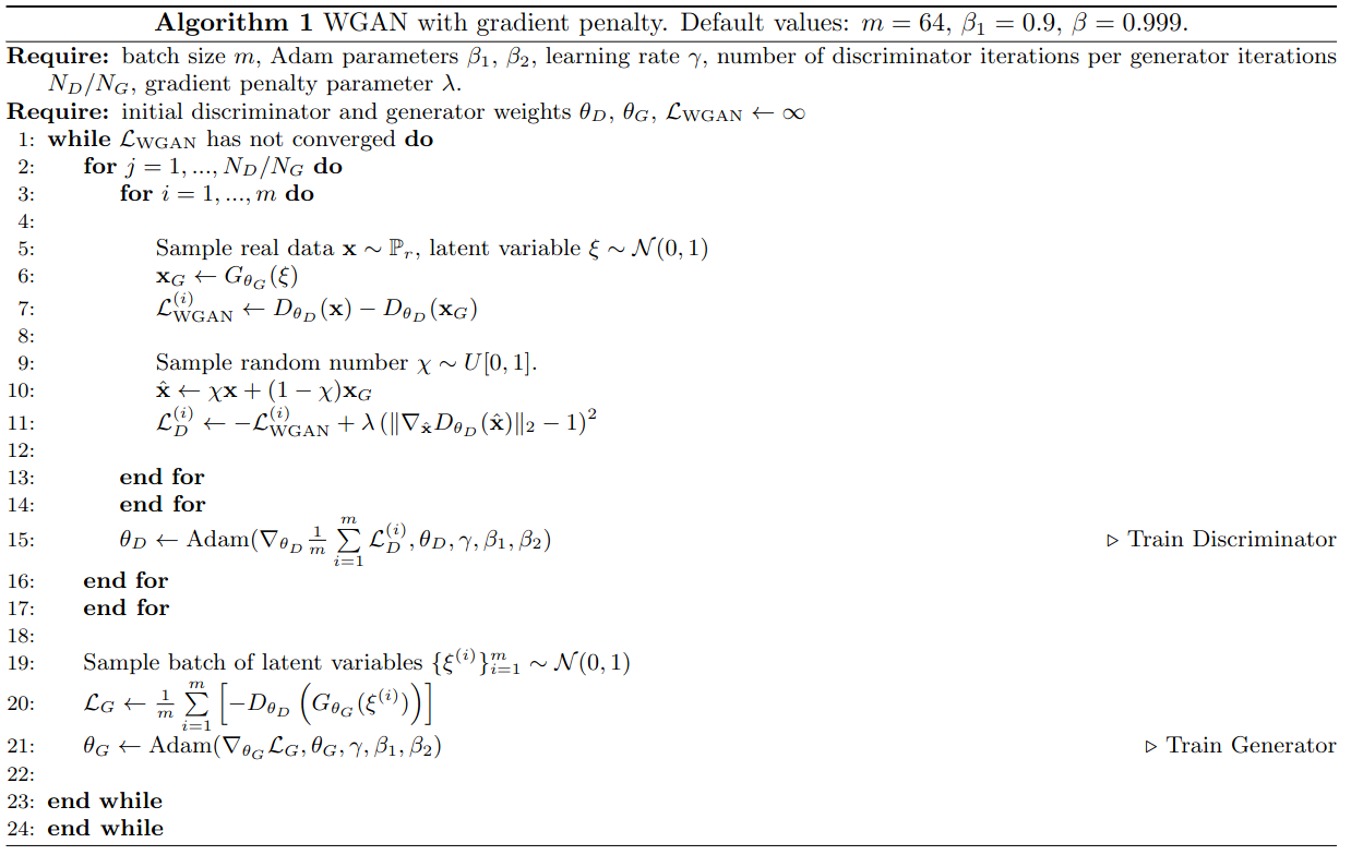
In the WGAN formulation, the output of the critic corresponds to a score that grades the origin of the input. Therefore, the critic is trained to output a higher score for the DNS input $\mathbf{x}$ than for its synthetic counterpart $\mathbf{x}_{G}$. The generator on the other hand, is trained to maximize the critic’s output for $\mathbf{x}_{G}$. The Wasserstein distance is incorporated into the discriminator loss function using the Kantorovich-Rubinstein duality Villani 2008. However, this restricts the critic $D(\cdot)$ to be a 1-Lipschitz function (i.e., the Lipschitz constant is one), which can be enforced by an additional gradient penalty term Gulrajani et al. 2017. The WGAN discriminator loss function then reads

$\displaystyle\mathcal{L}_{\rm D}=\underset{\mathbf{x}_{G}\sim P_{\rm G}}{\mathbb{E}}\left[D(\mathbf{x}_{G})\right]-\underset{\mathbf{x}\sim P_{\rm r}}{\mathbb{E}}\left[D(\mathbf{x})\right]+\lambda\underset{\hat{\mathbf{x}}\sim P_{\hat{\mathbf{x}}}}{\mathbb{E}}\left[\left(\|\nabla_{\hat{\mathbf{x}}}D\left(\hat{\mathbf{x}}\right)\|_{2}-1\right)^{2}\right],$

(48)

where $\mathbf{x}$ is sampled from the real, i.e., DNS data distribution $P_{\rm r}$ and $\mathbf{x}_{G}$ from the generator model distribution $P_{\rm G}$. The latter is given by $G\left(\mathbf{\xi}\right)$ with the random latent variable $\mathbf{\xi}\sim\mathcal{N}(0,1)$. The last term in (48) is the gradient penalty term, which enforces the 1-Lipschitz condition on the discriminator. The random samples $\hat{\mathbf{x}}$ are sampled from straight lines $\chi\mathbf{x}+(1-\chi)\mathbf{x}_{G}$ between pairs of $\mathbf{x}$ and $\mathbf{x}_{G}$, as proposed in by Gulrajani et al. Gulrajani et al. 2017. Here, $\chi\sim U[0,1]$, i.e., uniformly distributed between 0 and 1. The gradient penalty weight $\lambda$ is a hyperparameter. Moreover, the generator loss is given by

$\displaystyle\mathcal{L}_{\rm G}=-\underset{\mathbf{x}_{G}\sim P_{\rm G}}{\mathbb{E}}[D(\mathbf{x}_{G})].$

(49)

Finally, the Wasserstein loss function, which is given by

$\displaystyle\mathcal{L}_{\rm WGAN}=\underset{\mathbf{x}\sim P_{\rm r}}{\mathbb{E}}[D(\mathbf{x})]-\underset{\mathbf{x}_{G}\sim P_{\rm G}}{\mathbb{E}}[D(\mathbf{x}_{G})]\,,$

(50)

reflects the WGAN performance. We summarize the WGAN training procedure in Algorithm 1.

As discussed in the main text, we renormalize the DNS data to leverage the self-similar behavior of the CBL. For this, we renormalize the fluctuations of vertical velocity and buoyancy fields by their corresponding convective scales Deardorff 1970, see eqns. (4) in the main text, where the CBL height $h(t)$ is given by definition (1) in the main text. Further, the coordinates are measured in units of $h(t)$, i.e., $\tilde{x}=x/h$, $\tilde{y}=y/h$, $\tilde{z}=z/h$. By doing so, we fix the CBL height. This has implications for the horizontal extent of the normalized snapshots as the aspect ratio of the domain decreases over time. Hence, to compare two snapshots at two different $h/L_{0}$ with the same horizontal extend, one has to crop the snapshot with the smaller value of $h(t)/L_{0}$. In this way, we remove the first-order effects of the transient CBL growth in a fixed plane $\tilde{z}={\rm const}$. This process is illustrated in Fig. 8.

In panels (I–L), it can be seen that for sufficiently large values of $h/L_{0}$, this procedure produces horizontal slices with comparable flow patterns. The same does hold for the buoyancy fluctuations $b^{\prime}$ (not shown). It is these flow patterns that the GAN will be trained with to generate synthetic data.

The cutoff value of $h/L_{0}$, after which all re-normalized snapshots can be considered for the training routine, is determined by the following procedure. First, the individual up- and downdraft areas $A_{u}$ and $A_{d}$, given by values $w>0.95\max(w)$ and $w<0.95\min(w)$ respectively, are retrieved using the algorithm introduced in Suzuki and be 1985 via the OpenCV Itseez 2015 library implementation. Finally, we computed the Kullback-Leibler divergence (KLD) between the PDF $p$ of up- or downdrafts at $h/L_{0}$ with the final PDF $p_{\rm final}$ at $h/L_{0}=48.41$. For the updrafts, it is then given by

$\displaystyle D_{\mathrm{KL}}(p\|p_{\rm final})=\sum_{A_{u}}p(A_{u})\log\left(\frac{p(A_{u})}{p_{\rm final}(A_{u})}\right)\,.$

(51)

Figure 9 shows the KLD for the three planes over $h/L_{0}$. The slope of the KLD becomes less steep near $h/L_{0}=35.87$ (start of green shaded area). After this value, we consider all snapshots for the GAN training.

The normalized and cropped horizontal slices at the three heights are subsequently used to train three independent generative networks. For each height, $550$ snapshots are available for training. Moreover, we use data augmentation to increase the number of training samples to $32\cdot 550=17600$. For this, we consider a quarter of the renormalized DNS data as discriminator input. Hence, also the generator will be trained to generate a quarter of the original horizontal extent. Furthermore, we add rotations by angles of $\pi/2,\pi,3\pi/2$, reflections about the $\tilde{x}$- and $\tilde{y}$-axes, as well as combinations of $\pi/2$-rotations and $\tilde{x}/\tilde{y}$-reflections. This significantly increased the number of training samples, which resulted in better generator performances.

The GANs were trained for $2000$ epochs using the Adaptive moments (Adam) optimizer Kingma and Ba 2017. An early stopping routine ceased training after $300$ epochs of no improvement of the Wasserstein metric $\mathcal{L}_{\rm WGAN}$. Each run was performed on two NVIDIA A100 Tensor-Core GPUs and took up to 24 h to finish. The choice of GAN hyperparameters for the three planes is listed in Tab. 1. Figure 10 shows additionally the losses for both, the generator and the discriminator, together with the Wasserstein loss for all three GANs.

References

- Lenschow and Stephens (1980) D. H. Lenschow and P. L. Stephens, Boundary Layer Meteorol. 19, 509 (1980).
- Bodenschatz et al. (2010) E. Bodenschatz, S. P. Malinowski, R. A. Shaw, and F. Stratmann, Science 327, 970 (2010).
- Mellado (2017) J. P. Mellado, Annu. Rev. Fluid Mech. 49, 145 (2017).
- Atkinson and Wu Zhang (1996) B. W. Atkinson and J. Wu Zhang, Rev. Geophys. 34, 403 (1996).
- Bony et al. (2020) S. Bony, H. Schulz, J. Vial, and B. Stevens, Geophys. Res. Lett. 47, e2019GL085988 (2020).
- Madden and Julian (1972) R. A. Madden and P. R. Julian, J. Atmos. Sci. 29, 1109 (1972).
- Miura et al. (2007) H. Miura, M. Satoh, T. Nasuno, A. T. Noda, and K. Oouchi, Science 318, 1763 (2007).
- Ertel (1942) H. Ertel, Meteor. Z. 59, 1690 (1942).
- Deardorff (1972) J. W. Deardorff, J. Geophys. Res. 77, 5900 (1972).
- Arakawa (1974) W. H. Arakawa, A.and Schubert, J. Atmos. Sci. 31, 674 (1974).
- LeMone et al. (2019) M. A. LeMone, W. M. Angevine, C. S. Bretherton, F. Chen, J. Dudhia, E. Fedorovich, K. B. Katsaros, D. H. Lenschow, L. Mahrt, E. G. Patton, et al., Meteorol. Monogr. 59, 1 (2019).
- Tiedtke (1989) M. Tiedtke, Mon. Weather Rev. 117, 1779 (1989).
- Siebesma and Cuijpers (1995) A. P. Siebesma and J. W. M. Cuijpers, J. Atmos. Sci. 52, 650 (1995).
- Želi et al. (2021) V. Želi, G. Brethouwer, S. Wallin, and A. V. Johansson, Boundary Layer Meteorol. 178, 487 (2021).
- Wyngaard (2010) J. C. Wyngaard, Turbulence in the Atmosphere (Cambridge University Press, Cambridge, UK, 2010).
- Klingebiel et al. (2021) M. Klingebiel, H. Konow, and B. Stevens, J. Atmos. Sci. 78, 3205 (2021).
- Vogel et al. (2022) R. Vogel, A. L. Albright, J. Vial, G. George, B. Stevens, and S. Bony, Nature 612, 696 (2022).
- Ahlgrimm and Forbes (2014) M. Ahlgrimm and R. Forbes, Mon. Weather Rev. 142, 668 (2014).
- Becker et al. (2021) T. Becker, P. Bechtold, and I. Sandu, Q. J. R. Meteorol. Soc. 4388–4407 (2021).
- Hohenegger et al. (2023) C. Hohenegger, P. Korn, L. Linardakis, R. Redler, R. Schnur, P. Adamidis, J. Bao, S. Bastin, M. Behravesh, M. Bergemann, et al., Geosci. Model Dev. 16, 779 (2023).
- Siebesma et al. (2007) A. P. Siebesma, P. M. M. Soares, and J. Teixeira, J. Atmos. Sci. 64, 1230 (2007).
- Brenowitz and Bretherton (2018) N. D. Brenowitz and C. S. Bretherton, Geophys. Res. Lett. 45, 6289 (2018).
- Reichstein et al. (2019) M. Reichstein, G. Camps-Valls, B. Stevens, M. Jung, J. Denzler, N. Carvalhais, and Prabhat, Nature 566, 195 (2019).
- Kashinath et al. (2021) K. Kashinath, M. Mustafa, A. Albert, J.-L. Wu, C. Jiang, S. Esmaeilzadeh, K. Azizzadenesheli, R. Wang, A. Chattopadhyay, A. Singh, et al., Phil. Trans. R. Soc. A 379, 20200093 (2021).
- Fonda et al. (2019) E. Fonda, A. Pandey, J. Schumacher, and K. R. Sreenivasan, Proc. Natl. Acad. Sci. USA 116, 8667 (2019).
- Rasp (2020) S. Rasp, Bull. Am. Meteorol. Soc. 101, E1980 (2020).
- Beck and Kurz (2021) A. Beck and M. Kurz, GAMM Mitteilungen 44, e202100002 (2021).
- Yuval et al. (2021) J. Yuval, P. A. O’Gorman, and C. N. Hill, Geophys. Res. Lett. 48, e2020GL091363 (2021).
- Cheng et al. (2022) Y. Cheng, M. G. Giometto, P. Kauffmann, L. Lin, C. Cao, C. Zupnick, H. Li, Q. Li, Y. Huang, R. Abernathey, et al., J. Adv. Model. Earth Syst. 14, e2021MS002847 (2022).
- Guan et al. (2023) Y. Guan, A. Subel, A. Chattopadhyay, and P. Hassanzadeh, Physica D 443, 133568 (2023).
- Bretherton et al. (2022) C. S. Bretherton, B. Henn, A. Kwa, N. D. Brenowitz, O. Watt-Meyer, J. McGibbon, W. A. Perkins, S. K. Clark, and L. Harris, J. Adv. Model. Earth Syst. 14, e2021MS002794 (2022).
- Heyder and Schumacher (2021) F. Heyder and J. Schumacher, Phys. Rev. E 103, 053107 (2021).
- Heyder et al. (2022) F. Heyder, J. P. Mellado, and J. Schumacher, Phys. Rev. E 106, 055303 (2022).
- Dai and Hemri (2021) Y. Dai and S. Hemri, Mon. Weather Rev. 149, 3923 (2021).
- Leinonen et al. (2019) J. Leinonen, A. Guillaume, and T. Yuan, Geophys. Res. Lett. 46, 7035 (2019).
- Price and Rasp (2022) I. Price and S. Rasp, PMLR 151, 10555 (2022).
- Shamekh and Gentine (2023) S. Shamekh and P. Gentine, J. Adv. Model. Earth Syst. pp. 1–33, submitted (2023).
- Goodfellow et al. (2014) I. J. Goodfellow, J. Pouget-Abadie, M. Mirza, B. Xu, D. Warde-Farley, S. Ozair, A. Courville, and Y. Bengio, arXiv:1406.2661 (2014).
- Goodfellow et al. (2016) I. Goodfellow, Y. Bengio, and A. Courville, Deep Learning (MIT Press, Cambridge, USA, 2016).
- Mellado and Ansorge (2012) J. P. Mellado and C. Ansorge, Z. Angew. Math. Mech. 92, 1 (2012).
- Garcia and Mellado (2014) J. R. Garcia and J. P. Mellado, J. Atmos. Sci. 71, 1935 (2014).
- Brunton et al. (2020) S. L. Brunton, B. R. Noack, and P. Koumoutsakos, Annu. Rev. Fluid Mech. 52, 477 (2020).
- Ronneberger et al. (2015) O. Ronneberger, P. Fischer, and T. Brox, Lecture Notes in Computational Science 9351, 234 (2015).
- Witte et al. (2022) A. Witte, A. Herrington, J. Teixeira, M. J. Kurowski, M. J. Chinita, R. L. Storer, K. Suselj, G. Matheou, and J. Bacmeister, Mon. Weath. Rev. 150, 2339 (2022).
- Nash (1950) J. F. Nash, Proc. Natl. Acad. Sci. USA 36, 48 (1950).
- Arjovsky et al. (2017) M. Arjovsky, S. Chintala, and L. Bottou, arXiv:1701.07875 (2017).
- Deardorff (1970) J. W. Deardorff, J. Atmos. Sci. 27, 1211 (1970).
- Soares et al. (2004) P. M. M. Soares, P. M. A. Miranda, A. P. Siebesma, and J. Teixeira, Q. J. R. Soc. Meteorol. 130, 3365 (2004).
- Kupka and Muthsam (2017) F. Kupka and H. J. Muthsam, Living Rev. Comput. Astrophys. 3, 1 (2017).
- Carson and Smith (1975) D. J. Carson and F. B. Smith, in Advances in Geophysics (Elsevier, 1975), vol. 18, pp. 111–124.
- Siebesma and Holtslag (1996) A. P. Siebesma and A. A. M. Holtslag, J. Atmos. Sci. 53, 2354 (1996).
- Schumann and Moeng (1991) U. Schumann and C.-H. Moeng, J. Atmos. Sci. 48, 1758 (1991).
- Holtslag and Duynkerke (1998) A. Holtslag and P. G. Duynkerke (Royal Netherlands Academy of Arts and Sciences, 1998).
- Holtslag and Moeng (1991) A. A. M. Holtslag and C.-H. Moeng, Journal of the Atmospheric Sciences 48, 1690 (1991), URL https://doi.org/10.1175/1520-0469(1991)048<1690:edacti>2.0.co;2.
- van Ulden (1997) A. P. van Ulden, A. P.and Siebesma, Amer. Meteor. Soc p. 257–259 (1997).
- He et al. (2015) K. He, X. Zhang, S. Ren, and J. Sun, arXiv:1502.01852 (2015).
- Villani (2008) C. Villani, Optimal Transport: Old and New, Grundlehren der mathematischen Wissenschaften (Springer, Berlin, 2008), ISBN 9783540710509.
- Gulrajani et al. (2017) I. Gulrajani, F. Ahmed, M. Arjovsky, V. Dumoulin, and A. C. Courville, in Advances in Neural Information Processing Systems, edited by I. Guyon, U. Von Luxburg, S. Bengio, H. Wallach, R. Fergus, S. Vishwanathan, and R. Garnett (Curran Associates, Inc., 2017), vol. 30.
- Suzuki and be (1985) S. Suzuki and K. be, Comput. Graph. Image Process. 30, 32 (1985), URL https://doi.org/10.1016/0734-189x(85)90016-7.
- Itseez (2015) Itseez, Open source computer vision library, https://github.com/itseez/opencv (2015).
- Kingma and Ba (2017) D. P. Kingma and J. Ba, arXiv:1412.6980 (2017).