Multiscale Dynamic Graph Representation for Biometric Recognition with Occlusions
Abstract
Occlusion is a common problem with biometric recognition in the wild. The generalization ability of CNNs greatly decreases due to the adverse effects of various occlusions. To this end, we propose a novel unified framework integrating the merits of both CNNs and graph models to overcome occlusion problems in biometric recognition, called multiscale dynamic graph representation (MS-DGR). More specifically, a group of deep features reflected on certain subregions is recrafted into a feature graph (FG). Each node inside the FG is deemed to characterize a specific local region of the input sample, and the edges imply the co-occurrence of non-occluded regions. By analyzing the similarities of the node representations and measuring the topological structures stored in the adjacent matrix, the proposed framework leverages dynamic graph matching to judiciously discard the nodes corresponding to the occluded parts. The multiscale strategy is further incorporated to attain more diverse nodes representing regions of various sizes. Furthermore, the proposed framework exhibits a more illustrative and reasonable inference by showing the paired nodes. Extensive experiments demonstrate the superiority of the proposed framework, which boosts the accuracy in both natural and occlusion-simulated cases by a large margin compared with that of baseline methods. The source code is available here, or you can visit this website: https://github.com/RenMin1991/Dyamic-Graph-Representation
I Introduction
Deep learning methods have achieved great success in recent years, especially in the area of computer vision. Convolutional neural networks (CNNs) have been widely applied as a powerful tool for image classification and feature extraction [1, 2, 3, 4, 7, 5, 6]. CNNs are also universally applied to biometrics, including iris recognition [50, 48, 49], face recognition [8, 9, 10, 11, 51, 12] and so on.
However, biometric tasks are greatly influenced by the uncertain factors of illuminations, poses, movements, facial expressions, and occlusions. Among them, occlusion is one of the most common challenges in unconstrained situations [13, 14, 40], as shown in Fig. 1. In these situations, gaps between intraclass samples are significantly enlarged. The generalization ability of CNNs is greatly degraded due to the adverse effects of various occlusions.

To address the occlusion problem in biometric recognition, prior knowledge about occluded regions, which are usually represented as masks, is necessary for most existing biometric recognition methods [47, 46, 48, 39, 40]. In these methods, the features of occluded areas are suppressed during matching according to the masks. However, pixel-wise labeling of masks is error-prone, and the errors are accumulated into inaccurate recognition results. More importantly, for deep learning-based methods, the features of occluded areas cannot be suppressed after feature extraction by low-level masks in CNNs where high-level feature vectors are mostly yielded from the complete images. It is experimentally demonstrated in Section IV-C that masking the occluded areas before feature extraction is suboptimal.
In the conference version of this paper [31], we proposed a novel unified framework named DGR for handling occlusion problems in biometrics. Basically, CNNs are adopted to extract deep features, and a group of deep features reflected on certain subregions are recrafted into a FG. Each node inside FG is deemed to characterize a specific local region of the input sample, and the edges imply the co-occurrence of non-occluded regions. By analyzing the similarities of the node representations and measuring the topological structures stored in the adjacent matrix, the proposed framework leverages dynamic graph matching to judiciously discard the nodes corresponding to the occluded parts. As a result, the similarity between intraclass samples can be significantly increased. In addition, the proposed framework provides the underlying reasons for the recognition decisions. The matched or non-matched nodes in the proposed dynamic graph method provide more illustrative and reasonable matching results, which serve as a support for decisions. For example, the probe face image differs from gallery images mainly in the left eye and nose regions, which can be visualized through dynamic graph matching so that it can be considered as an imposter. In other words, FG can explicitly show the reserved local regions and the similarities between these local regions. Hence, the output of the framework can be better perceived.

The graph model and CNNs are seamlessly combined: CNNs produce the feature maps for the graph generator to construct graphs, which are called FG. The graph generator would automatically choose a subset of spatial nodes from the feature maps, convey edges to express the spatial relationships between nodes and finally assemble them together as FG. A novel deep graph model named squeeze-and-excitation graph attention networks (SE-GAT) is proposed to enhance the discrimination of FG. During the matching stage, dynamic graph matching is implemented. The nodes corresponding to the occluded parts are discarded accordingly by analyzing the similarities of the node representations and measuring the topological structures, as shown in Fig. 2. The proposed framework is remarkably resilient to variations in the locus and ratio of occluded regions because the local features are activated or not through node selection in dynamic graph matching.

This paper first extends our previous work by introducing the multiscale strategy as shown in Fig. 3. The representations of nodes from one single layer can only ingest contexts from receptive fields of the same size. Thus, the multiscale strategy is further incorporated to attain more diverse nodes representing regions of various sizes. The primitive FGs are subsequently reorganized in a hierarchical manner for escalated dynamic graph matching. FGs are generated from feature maps of different layers. Multiscale content representations and relationship representations are contained in multiscale FGs, and all of these FGs of different scales are summarized together in the framework. Node features yielded from different layers correspond to different scales of local regions of the input image. Edges from different layers represent topological structures of different scales. Hence, the features contained in multiscale FGs representation are much more abundant than those in single-scale representation.
Second, the novel matching mechanism is of commendable scalability, which can be applied to both deep learning-based and handcrafted methods for biometric recognition. The proposed dynamic graph matching is applied to the handcrafted features for a more convincing comparison with the masking strategy. More analyses and experiments are provided later to exhibit the characteristics of the proposed multiscale FGs and dynamic graph matching.
The major contributions of this paper can be summarized as follows:
1. We develop a novel framework for solving occlusion problems in biometrics that integrates the merits of both CNNs and graph models. The proposed framework provides a novel strategy to deal with occlusions.
2. The proposed framework boosts the recognition performance by a large margin in comparison with baseline methods, especially in occluded scenarios.
3. The decisions made by our framework are more convincing and reasonable than vanilla CNN-based methods due to providing the underlying reasons for inference.
The remainder of this paper is organized as follows: Section II presents a literature review of related works. The proposed framework is detailed in Section III. The configurations and results of experiments are presented in Section IV. Finally, the conclusion of this paper is presented in Section V.
II Related Works
In this section, we will briefly introduce the biometric approaches based on CNNs as a baseline, the handcrafted graph representation methods as references, deep graph neural networks (GNNs) as tools and the multiscale strategy in computer vision research.
Iris recognition has attracted increasing attention as one of the most accurate and reliable methods for identity authentication. Recently, CNN-based methods for iris recognition have been presented. The parameters of the deep learning model are tuned through data fitting. DeepIris is proposed in [50] for heterogeneous iris matching. The fully convolutional network (FCN)-based model named UniNet is proposed for iris recognition in [48]. MaxoutCNNs is proposed for iris and periocular recognition in [49]. However, occlusion problems, which are common for the iris, remain the bottleneck preventing improvement of the recognition performance. Almost all existing CNN-based methods adopt the masking strategy, which is borrowed from conventional methods. However, the masking strategy is not suitable for the CNN architecture since the non-iris regions cannot be excluded after feature extraction.
The first method for face representation based on CNN was proposed by Taigman et al. [8]. A framework employing multiple convolutional networks was proposed by Sun et al. [9]. The triplet loss function is applied to produce 128-D face embedding representations in [10]. A light-weight convolutional architecture is proposed for face recognition in [51]. Recently, several approaches for facial feature embedding enhancement have been proposed, including SphereFace [11], ArcFace [12], CosFace [15] and so on.
There are also region-based or partial-based models for face recognition [16, 17, 40, 41, 42]. However, similar to the masking strategy, all of these approaches need to set apart the occluded regions of face images before feature extraction.
Graph-based methods for biometrics. There are some existing handcrafted graph-based methods for biometrics, including iris [18], face [19], periocular [20], ear [19] and hand vein [21]. Although these handcrafted methods may have inspired us, the methods cannot be directly adopted in deep learning-based frameworks.
Deep learning approaches on graphs. Graphs are ubiquitous in the world. GNNs are introduced as recursive neural networks in [24, 25] to handle graph data. Recently, the generalization of the convolutional operation has attracted increasing attention. Approaches in this direction can be roughly categorized as spectral approaches and nonspectral approaches [23]. The spectral approaches [26, 27] work with spectral representations of graphs. The nonspectral approaches [28, 29, 30] define convolutional operations directly on graphs. Graph attention networks (GAT) [43] introduce the attention mechanism to deep graph models.
Deep graph matching methods have been commonly studied recently [56, 57, 58, 59]. Comparing to general deep learning based graph matching methods, the proposed dynamic graph matching is designed to handle graphs with dynamic nodes and edges rather than fixed structure, because the structure of FG changes according to the occluded parts. Besides, biometric recognition with occlusions in the real world requests to generalize on various occlusions, which is a challenge for the data-driven methods.
Multiscale strategy. The multiscale strategy is an effective approach that has been widely used in the literature. Multiscale information is utilized in SIFT [32] by building an image pyramid for more stable and scale-invariant localization and description of key points. Bay et al. [36] follow the multiscale approach for key point detection and description.
The multiscale approach is also an effective strategy for deep learning frameworks. For example, information on different scales is fused together in [33] for deep learning-based semantic segmentation. The coarse, global-scale information from deep layers and fine, local-scale information from shallow layers are both useful. The strategy of the multiscale pyramid is introduced for object detection in [34], where multiscale feature vectors are aggregated to process objects of different scales.
III Multiscale Dynamic Graph Representation

In this section, we briefly introduce the overall framework to handle the occlusion problems in biometrics. Two crucial components of MS-DGR include the graph generator and SE-GAT, which are elaborated separately. Next, a novel loss function designed for supervising the training of dynamic graph feature learning and the strategy of dynamic graph matching are introduced.
III-A Overall Framework
In the proposed framework, input images are sent to a network that contains several convolutional blocks as shown in Fig. 3. Each convolutional block consists of several convolutional layers and pooling layers. Feature maps of different scales generated by convolutional blocks are sent to graph blocks. FG built upon these feature maps are generated by the graph blocks, in which nodes contain the local patterns and the weighted edges convey the topological structures of nodes.
The graph block consists of the graph generator and SE-GAT, as shown in Fig. 4(a). FGs are generated from feature maps by the graph generator before being sent to SE-GAT, which is a hierarchical feature extractor based on GAT for graph-style inputs. FGs extracted by SE-GAT have two components: i. the content messages of subregions contained in the feature vectors of nodes and ii. the topological structure messages contained in the adjacent matrix of the graph. Through the multiscale strategy, nodes perceive both coarse and fine local patterns, and the adjacent matrices encode topological structures at different scales.
As shown in Fig. 3, three graph blocks are integrated into CNNs, and the global feature is produced by the CNNs. Our framework can be incorporated into any CNNs by combining the global feature and FGs.
Finally, two kinds of loss functions are applied during training. The global feature is passed to a classification layer for measuring classification loss. FGs processed through SE-GAT are sent to a novel graph triplet loss function. The novel loss function provides a new way to measure the similarity of two graphs. Both the similarity of the node representations and the topological structures are taken into consideration.
III-B Graph Generator
There are two steps to generate a FG from feature maps, as shown in Fig. 4(b). The first step is to generate the nodes, i.e., to regress the spatial locations of nodes and selecting from the feature maps. The second step is generating the edges/adjacent matrix according to the relationships of nodes.
The nodes of a FG are selected from the feature map. Firstly, a smaller architecture is adopted to find the spatial locations of the essential features within the feature map. The smaller architecture, which is named spatial location network (SLN), takes the feature map as input. Its output is the spatial coordinates of the selected features. SLN detects spatial locations of interest points through regression. This network is trained to find the most discriminative features in the feature map. It transforms the feature map into the spatial coordinates of nodes. Following the conventional practice of CNNs, it consists of two convolutional layers, two pooling layers, and two fully connected layers (its layer configurations are shown in Tab. I). The dimension of the feature map is decreased gradually during the first five layers of the SLN. In the last fully connected layer, the feature is transformed into the spatial coordinates of nodes.
Then, CNN features are extracted from the localized points of interest. These selected features are the representations of nodes. One node corresponds to one location. The feature selection is realized by bilinear interpolation according to the spatial coordinates:
| (1) |
where f is the feature vector, F is the feature map, are the spatial coordinates which are the output of SLN, is the index of the feature vector and , is the number of channels of the feature map. Now, the nodes of a FG have been generated.
| Layer | Kernel Size | Stride | Input Size | Output size |
|---|---|---|---|---|
| Pool1 | ||||
| Conv1 | ||||
| Pool2 | ||||
| Conv2 | ||||
| FC1 | – | – | ||
| FC2 | – | – |
The edges/adjacent matrix of a FG is generated according to the spatial relationships between nodes. For two nodes of FG, the weight of the edge between them is generated by the spatial Gaussian kernel function:
| (2) |
where is a adjacent matrix, is the number of nodes, are the spatial coordinates of two nodes, and is the scale of the receptive field of each node. Hence, the edge represents the spatial relationship of the two nodes. The closer the two nodes are to each other, the higher the weight of the edge is. If the distance between the two nodes is larger than the scale of the receptive field, the weight is 0 (there is no relationship between them). In this way, the edges/adjacent matrix of FG have been generated.
There should be an information interaction between two nodes in the graph neural network if their receptive fields are overlapped. On the other hand, if the distance between two nodes is higher than R, their receptive fields are not overlapped, and the two nodes should not be connected.
In general, the SLN constructs the feature vectors affiliated with critical regions as nodes of FG. The spatial Gaussian kernel function establishes edges among nodes.
III-C Squeeze-and-Excitation Graph Attention Networks
SE-GAT is a novel model based on GAT [43]. It consists of two kinds of layers: the squeeze-and-excitation (SE) layer and graph attention (GAT) layer. We describe them as follows:
The SE layer is a generalized version of the squeeze-and-excitation block [6], which is effective in CNNs. The same channel of different feature vectors represents the energy of the same pattern at different positions of the input image. The SE layer enhances the important channels and suppresses the nonsignificant channels by assigning weights. As shown in Fig. 5, the average energy of each channel of nodes is calculated by the global pooling operation:
| (3) |
where z is the squeezed vector, G is FG, is the number of nodes, is the index of the feature vector of each node and . Two fully connected layers are used to make use of the global information:
| (4) |
where s is the scale vector, are parameters of the two fully connected layers, and are activation functions. The scale vector s is used to rescale each channel of FG:
| (5) |
where is the rescaled feature vector, is the channel index of the feature vector and , is the index of nodes and .

The GAT layer is a modified variant of the layer in [43]. The weights of different edges of FG are different, rather than the same, in [43]. The formulation of the layer is given as follows:
| (6) |
| (7) |
| (8) |
where is the output vector, is the input vector, is a nonlinear activation function, is the set of first-order neighbors of node (including ), is the attention value between node and node , and are the parameters of the GAT layer, is the adjacent matrix of the input graph, and indicates concatenation.
The module of SE-GAT is shown in Fig. 4(c). As the residual structure has been proven to be effective for CNNs [7], we extend it to the graph model in SE-GAT. The residual block in the SE-GAT module has four layers, two of which are SE layers, and the rest are GAT layers. A dimension reduction layer is adopted to reduce the dimensions of feature vectors of nodes:
| (9) |
where is the parameter matrix, is an activation function, and is the output vector. Finally, FG is extracted for matching.
III-D Graph Triplet Loss Function
As described above, FG consists of node representations and adjacent matrices. Hence, the similarity between the outputs of two samples consists of two terms:
| (10) |
where is the semantic similarity and is the relationship similarity.
| (11) |
where represents the cosine similarity, and are the concatenation of all feature vectors of FGs and global features generated by fully connected layers.
| (12) |
where is the number of FGs in a single input image extracted by the network, is the number of nodes of the -th FG, and are the adjacent matrices of the -th FGs of two samples. Finally, the graph triplet loss is:
| (13) |
where is the similarity between anchor sample and negative sample, is the similarity between anchor sample and positive sample, and is a predefined positive margin and set to 1 during training.
III-E Dynamic Graph Matching
Given two FGs, and , from the same scale level extracted from two image samples, we firstly filter out dissimilar nodes by using the mean of cosine similarities of corresponding nodes as the threshold, which can be calculated as follows:
| (14) |
where and are the node features of and , and is the number of nodes in each FG. Then, if the similarity of a node pair is less than the , this node pair is removed from the two FGs:
| (15) |
where represents the remove operation according to the , and the dynamic FGs and are built. Finally, multiscale dynamic FGs of two samples are built according to Eq. 15.
The variance of occluded parts is much larger than the variance of non-occluded biometric images. The similarity between the occluded region and non-occluded region is very likely to be lower than that between non-occluded regions. Hence, node pairs with lower similarities are removed to adaptively select features. The threshold set by the mean of similarities provides a straightforward and effective way to build dynamic FGs.
IV Experiments
Two modalities, iris and face, are selected to evaluate the proposed framework. Experiments on non-occluded and occluded instances are both taken into consideration. Thorough experiments are launched to analyze the proposed framework, including comparison with other state-of-the-art methods in both non-occluded and occluded biometric cases, the comparison to masking strategy, the evaluation of different scales, the evaluation under different node number settings and ablation studies. In addition, the visualization of FGs further provides the underlying reasons for recognition decisions.
| Layer | Kernel Size | Stride | Padding | Input Size | Output size |
| Conv Block 1 | |||||
| Conv1 | |||||
| Pool1 | – | ||||
| Conv2 | |||||
| Pool2 | – | ||||
| Conv3 | |||||
| Conv Block 2 | |||||
| Pool3 | – | ||||
| Conv4 | |||||
| Conv Block 3 | |||||
| Pool4 | – | ||||
| Conv5 | |||||
| FC Block | |||||
| Pool5 | – | ||||
| FC1 | – | – | – | ||
| FC2 | – | – | – | ||
IV-A Experiments of Iris Recognition
IV-A1 Protocols and Databases
A light-weight CNNs is used for iris experiments. Its layer configuration is shown in Tab. II, and the multiscale FGs consist of three scales: small scale, medium scale, and large scale. Each scale is obtained from a different convolutional block of the CNNs. The number of nodes decreases along with the scales of the FG. The node numbers of the small-, medium-, and large-scale FG are set as 64, 32, and 16, respectively. Stochastic gradient descent with momentum is adopted for optimization. Training is started with a learning rate of 0.001 and divided by 2 every 10 epoch and stopped at the 40th epoch. The size of the mini-batch is 64. The weight decay is 0.0001.

| ND-LG4000 | CASIA-Distance | CASIA-M1-S2 | CASIA-M1-S3 | CASIA-Lamp | ||||||
| FRR | EER | FRR | EER | FRR | EER | FRR | EER | FRR | EER | |
| log-Gabor [47] | 35.90% | 3.25% | 38.33% | 9.98% | 45.03% | 6.35% | 59.84% | 9.14% | 42.93% | 7.63% |
| OMs [46] | 17.95% | 2.08% | 28.88% | 4.30% | 16.68% | 3.34% | 22.14% | 5.03% | 19.30% | 3.30% |
| UniNet [48] | 13.71% | 2.80% | 21.95% | 3.65% | 13.17% | 2.63% | 14.58% | 2.80% | 14.92% | 3.89% |
| MaxoutCNNs [49] | 9.89% | 1.77% | 19.61% | 2.22% | 13.81% | 1.81% | 15.26% | 1.92% | 14.48% | 2.78% |
| Ours-CD | – | – | 9.93% | 2.17% | 7.33% | 0.82% | 8.65% | 0.87% | 5.78% | 0.58% |
| Ours-WD | 2.76% | 0.58% | 5.98% | 1.55% | 5.86% | 0.71% | 6.40% | 0.75% | 3.85% | 0.46% |
Three performance indexes are adopted to evaluate the recognition methods:
False acceptance rate (FAR):
| (16) |
where is the number of false accepted pairs, is the total number of negative pairs.
False rejection rate (FRR):
| (17) |
where is the number of false rejected pairs, is the total number of positive pairs.
Equal error rate (EER): EER is the working point on the DET curve where FAR equals to FRR.
For all iris images, the preprocessing procedure contains three steps: 1) eye detection by Haar-like Adaboost detectors [44], 2) iris boundary localization using the method in [45], and 3) iris normalization by rubber sheet model [38]. Circular iris images are normalized to a rectangle with resolution.
Five databases are used for experiments:
(1) ND CrossSensor Iris 2013 Dataset-LG4000 (ND-LG4000) [54]. This database is one of the most popular iris databases for iris recognition research. It contains 29,986 iris samples from 1,352 classes. The training set of this database consists of images of the first 676 classes. The test set, after removing some falsely normalized images, consists of the remaining 676 classes and contains 114,243 genuine pairs and 57,554,187 imposter pairs.
(2) CASIA Iris Image Database V4-Distance (CASIA-Distance) [53]. Images of this database are acquired from 3 meters away. It contains 2,446 iris samples from 284 classes. The training set of this database consists of images of the first 142 classes. The test set, after removing some falsely normalized images, consists of the remaining 142 classes and contains 12,617 genuine pairs and 1,695,859 imposter pairs.
(3) CASIA-Iris-M1-S2 (CASIA-M1-S2) [53]. Images of this database are acquired by mobile devices at three different distances. It contains 6,000 iris samples from 400 classes. The training set of this database consists of images of the first 200 classes. The test set consists of the remaining 200 classes and contains 21,000 genuine pairs and 4,477,500 imposter pairs.
(4) CASIA-Iris-M1-S3 (CASIA-M1-S3) [53]. Images of this database are acquired by mobile devices, different from CASIA-Iris-M1-S2. It contains 3,600 iris samples from 720 classes. The training set of this database consists of images of the first 360 classes. The test set consists of the remaining 360 classes and contains 3,600 genuine pairs and 1,615,500 imposter pairs.
(5) CASIA Iris Image Database V4-Lamp (CASIA-Lamp) [53]. This database contains 16,212 iris samples from 819 classes. A lamp close to the subject was turned on/off to introduce elastic deformation of the iris due to pupil expansion and contraction under different illumination conditions. The training set of this database consists of the first 409 classes. The test set, after removing some falsely normalized images, consists of the remaining 410 classes and contains 76,387 genuine pairs and 32,700,296 imposter pairs.
IV-A2 Comparisons to State-of-the-Art Approaches
The proposed method is compared with four state-of-the-art approaches: log-Gabor [47], ordinal measures (OMs) [46], UniNet [48] and MaxoutCNNs [49]. Handcrafted approaches and deep learning approaches are both taken into consideration. Open source implementation of USIT11 1 http://www.wavelab.at/sources/Rathgeb16a/ of log-Gabor [47] is adopted. We reproduced OMs in [46], and have tried our best to optimize the parameters for fair comparison. Authoritative implementations of UniNet [48] and MaxoutCNNs [49] are used, but the parameters are retrained following the configurations of experiments of this paper, and we have tried our best to optimize the models.
Two test configurations are incorporated to evaluate the proposed method: within-database (WD) and cross-database (CD) configuration. In the within-database (WD) configuration, models trained on ND-LG4000 were utilized as the pretrained model, and the models were fine-tuned on the other databases. In the cross-database (CD) configuration, ND-LG4000 was utilized as training set, and the trained models were tested without any fine-tuning process. The purpose of cross-database (CD) configuration is to evaluate the generalization capability of the proposed method.
The results are shown in Fig. 6 and Tab. III. Significant improvements from the proposed framework can be found for all five databases.
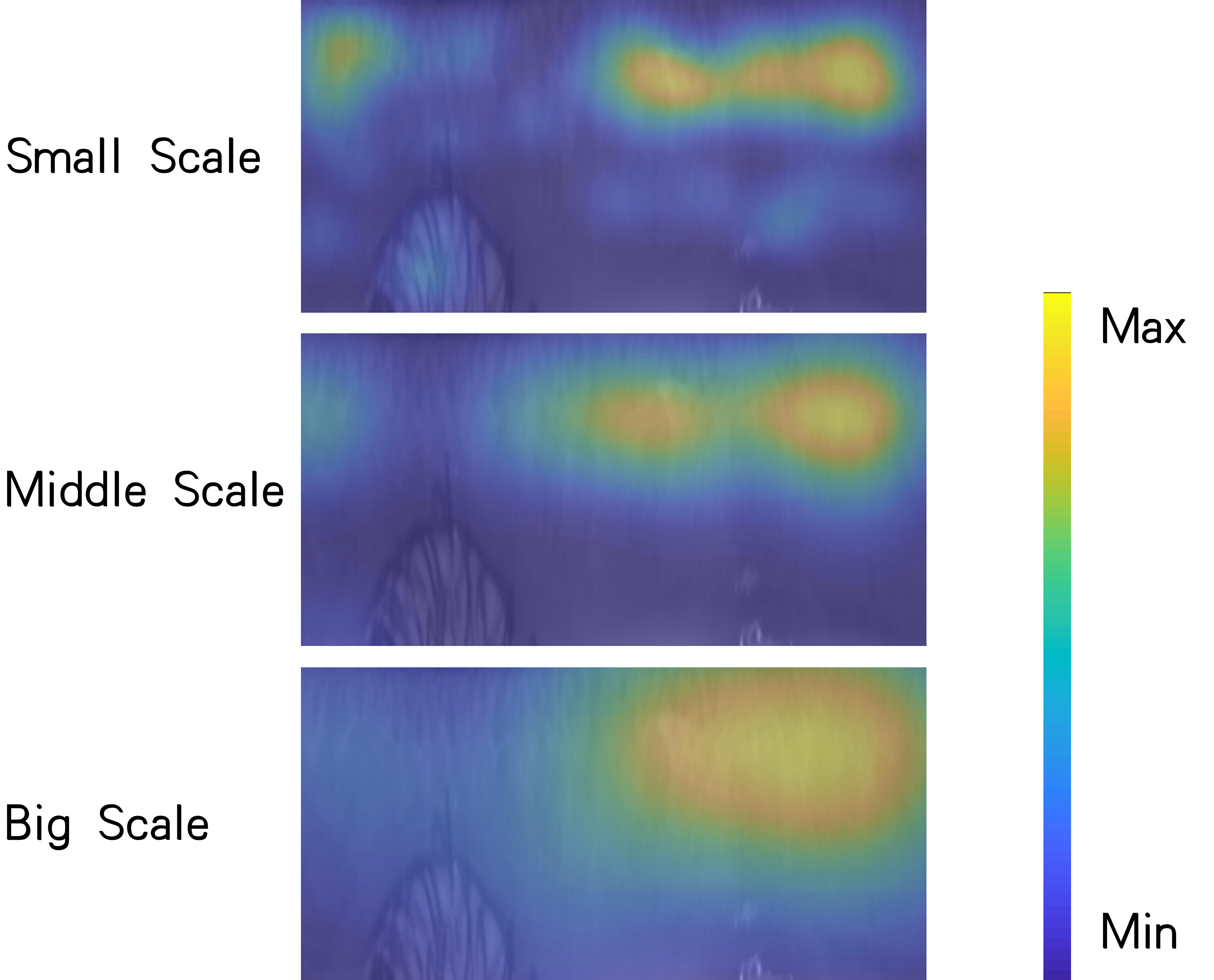
The saliency map of FGs of an iris sample from CASIA-Lamp is visualized in Fig. 7. Occluded regions caused by eyelids and eyelashes, which are useless for iris recognition, are suppressed. The small-scale FG focuses on local area patterns, and the large-scale FG focuses on large region patterns.
IV-A3 Occluded Iris Recognition
The occluded iris recognition experiment is launched on two databases. The first is the test database of ND CrossSensor Iris 2013 Dataset-LG4000. Special areas of iris samples are covered by random noise to simulate the occluded situations on this database, as shown in Fig. 8. The second is CASIA Iris Image Database V4-Thousand [53]. This database contains 20,000 iris samples from 2,000 classes. Various real occlusions, including eyelid, eyelash, and light spot, are contained in this database, as shown in Fig. 9.
For the test database of ND CrossSensor Iris 2013 Dataset-LG4000, the replaced areas are set according to the locations of eyelids and eyelashes in normalized iris images. Two kinds of occlusion situations shown in Fig. 8 are randomly selected with the same probability for a special iris sample, while the percentage of covered area remains the same. Masks, which contain the prior knowledge of the occluded region, are unavailable in these experiments for fair comparison. Comparisons to mask strategy are presented in Section IV-C.
Two protocols are adopted in the experiments on ND CrossSensor Iris 2013 Dataset-LG4000: (1) the occluded areas are cropped before feature extraction (the pixels of occluded areas are set to 0 if the input shape of the recognition model is constant), and (2) the occluded areas are also fed to the feature extractor. Note that none of the models used in this experiment are trained on the occluded database.


The results of two test protocols under occluded areas are shown in Tab. IV. The performance gap of the proposed framework between protocols (1) and (2) is much smaller than that for the other methods. For handcrafted approaches, the performance of protocol (2) is degraded because features extracted from occluded regions are interfused. For the deep learning-based methods, occluded regions of protocol (2) significantly increase the distance between intraclass samples, and the generalization abilities of these models in occluded situations are quite limited.
| FRR@FAR=0.1% | EER | |
|---|---|---|
| log-Gabor (1) [47] | 26.73% | 7.05% |
| log-Gabor (2) [47] | 41.76% | 27.25% |
| OMs (1) [46] | 16.72% | 5.3% |
| OMs (2) [46] | 38.67% | 26.29% |
| UniNet (1) [48] | 5.81% | 3.98% |
| UniNet (2) [48] | 45.33% | 8.32% |
| MaxoutCNNs (1) [49] | 76.25% | 9.61% |
| MaxoutCNNs (2) [49] | 73.68% | 21.8% |
| Ours (1) | 2.28% | 1.03% |
| Ours (2) | 1.48% | 0.80% |
An additional experiment is conducted to evaluate the influence of the occluded areas on the proposed framework. The performance of the proposed framework under different occluded sizes is provided in Fig. 10. It is not surprising to observe that the performance of the proposed framework degrades when the occlusion size grows. The performance declines dramatically only when the occluded areas are over 40%.One possible reason for this is that the threshold value of dynamic matching is set by the mean of similarities of nodes, as described in Section III-E, which means that the expected percentage of node removal is approximately 50%. The proposed framework can function well when the percentage of the occlusion area is lower than 50%, but features of occluded areas may be introduced when the percentage of the occluded area is higher than 50%.
This phenomenon indicates that the strategy of dynamic matching is not optimal when the occlusion is extremely serious, which is a limitation of the proposed framework.

| FRR@FAR=0.1% | EER | |||||
|---|---|---|---|---|---|---|
| USABLE_IRIS_AREA | 70%-80% | 60%-70% | 50%-60% | 70%-80% | 60%-70% | 50%-60% |
| log-Gabor [47] | 18.60% | 27.26% | 27.14% | 4.85% | 7.03% | 7.27% |
| OMs [46] | 17.65% | 23.99% | 24.86% | 4.71% | 6.49% | 6.87% |
| UniNet [48] | 10.24% | 22.69% | 24.40% | 2.65% | 4.32% | 6.38% |
| MaxoutCNNs [49] | 86.81% | 86.91% | 89.65% | 14.70% | 15.22% | 15.73% |
| Ours | 2.21% | 3.75% | 5.25% | 0.65% | 1.15% | 1.99% |
To test the performance of the proposed framework on iris images with real occlusions, the experiments are conducted on CASIA Iris Image Database V4-Thousand. The samples in this database are divided into subsets according to their USABLE_IRIS_AREA defined by ISO/IEC 29794-6 [60]:
| (18) |
where is the area of iris, is the area of occluded iris. In this experiment, is calculated according to the inner and outer boundary of iris, is calculated according to the ground truth iris mask. The USABLE_IRIS_AREA is the fraction of the iris portion of the image that is not occluded. Three subsets are adopted for testing, the range of USABLE_IRIS_AREA are 70% - 80%, 60% - 70%, and 50% - 60% respectively. To evaluate the generalization ability of the proposed method, the models in this experiment are not re-trained on CASIA Iris Image Database V4-Thousand.
The results are shown in Tab. V. The proposed framework significantly outperforms the compared methods in all three subsets. The proposed framework works well in both simulated and real occlusion scenarios because the nodes corresponding to occluded regions are adaptively removed. The results indicate that the proposed framework offers desirable generalization ability in real-world occluded situations.
IV-B Face Recognition Experiments
| TAR@FAR=1% | TAR@FAR=0.1% | TAR@FAR=0 | 100%-EER | |
| LFW | ||||
| ArcFace (ResNet50) [12] | 99.64% | 99.33% | 97.23% | 99.56% |
| ArcFace (ResNet101) [12] | 99.75% | 99.54% | 97.90% | 99.67% |
| Ours (ResNet50) | 99.67% | 99.20% | 98.15% | 99.56% |
| Ours (ResNet101) | 99.87% | 99.71% | 98.22% | 99.77% |
| MegaFace | ||||
| ArcFace (ResNet50) [12] | 96.92% | 94.23% | 89.36% | 87.64% |
| ArcFace (ResNet101) [12] | 98.61% | 96.22% | 78.18% | 75.16% |
| Ours (ResNet50) | 97.26% | 95.15% | 93.91% | 90.62% |
| Ours (ResNet101) | 98.47% | 96.69% | 89.80% | 83.99% |

IV-B1 Comparisons to State-of-the-Art Methods
The proposed method is compared with ArcFace [12], which is a state-of-the-art method for face recognition. ResNet50 and ResNet101 are utilized as backbone. MS-DGR is integrated into these models. For ResNet50, the first convolutional block contains 14 convolutional layers, the second consists of 28 convolutional layers, and the third consists of the 6 remaining convolutional layers. For ResNet101, the first convolutional block contains 32 convolutional layers, the second consists of 60 convolutional layers, and the third consists of the 6 remaining convolutional layers. The node numbers are set to 64, 32 and 16 when constructing FGs from respective feature maps. Stochastic gradient descent with momentum is adopted for optimization. Training is started with a learning rate of 0.01 and divided by 10 every 10 epoch and stopped at the 30th epoch. The size of the mini-batch is 128. The weight decay is 0.0001.
The data preprocessing method of ArcFace [12] is used, and the training databases22 2 https://github.com/deepinsight/insightface of ArcFace [12] are adopted for fair comparison. Labeled Faces in the Wild [52] (LFW) and MegaFace [37] are selected as the test sets.
The results are shown in Tab. VI. The proposed method is better than ArcFace [12] in most cases. Along with the decreasing FAR, the advantage of our method becomes more salient, which indicates the effectiveness of the proposed graph module in our framework for face recognition.
Small-scale FGs of example face images are visualized in Fig. 11. The first row shows the 10 pairs of nodes with the highest similarity scores. The second row shows the 10 node pairs with the lowest similarity scores. These examples show the regions that are deemed most similar/dissimilar by the framework, which is the underlying reason for recognition decisions. These examples show that FGs produce more illustrative and reasonable inferences by showing local patch similarities with representations. For example, in the left pair of images, the most similar nodes pairs are uniformly distributed over the whole face since the poses and expressions are similar. The most dissimilar nodes scatter around the eyes because of the glasses.
Meanwhile, these examples show that the SLN, which detects the spatial locations of nodes, is robust to illumination (the left pair of Fig. 11), head pose (the middle pair of Fig. 11), and expression (the right pair of Fig. 11). SLN chooses the discriminative regions of the image pairs in these scenarios. For example, in the middle pair of images, nodes of the right image are concentrated on the right-half face because the left-half face is not visible.
IV-B2 Occluded Face Verification
Light CNN (LCNN) [51] is adopted to build the architecture for occluded face recognition. The LCNN-9 version that contains 9 convolutional layers is selected.
Similar to ArcFace experiments, the LCNN model is split into three convolutional blocks for the integration of graph modules. The first convolutional block contains 5 convolutional layers, the second consists of 2 convolutional layers, and the third consists of the remaining 2 convolutional layers. The node numbers of the three FGs are set as 128, 64, and 64. Stochastic gradient descent with momentum is adopted for optimization. Training is started with a learning rate of 0.001 and divided by 2 every 10 epoch and stopped at the 40th epoch. The size of the mini-batch is 128. The weight decay is 0.0001.
The data preprocessing method of LCNN is used, and the training set is CASIA-WebFace [9]. Horizontal mirror operation is conducted for data augmentation because faces have a nearly symmetric structure.
Both simulated and real occlusions are taken into consideration. For simulated occlusions, a simulated occluded face database named Occluded-LFW, which is based on the Labeled Faces in the Wild [52] (LFW) database, is used for evaluation. LFW contains 13,233 images from 7,749 individuals. Face images of LFW vary in terms of pose, expression, and illumination. After the same preprocessing of the training images, three kinds of simulated occlusions are taken into consideration, as shown in the first three rows of Fig. 12. In the first case, rectangular areas of face images are covered by random noises to simulate the occluded situations during this experiment. Four regions in the first row of Fig. 12, right, left, upper, and bottom, are randomly covered with the same probability during this experiment. In the second case, face images are covered by random shapes of noises. Four shapes shown in the second row of Fig. 12 are randomly selected with the same probability during this experiment. The location of the noises is also randomly selected. In the third case, four kinds of masks, the surgical mask, N95, the cloth mask, and the gas mask, are overlaid on the face images according to face landmarks. The four kinds of masks are randomly selected with the same probability during this experiment. We follow the Labeled Faces in the Wild (LFW) benchmark protocol33 3 http://vis-www.cs.umass.edu/lfw/pairs.txt, where 3,000 positive pairs and 3,000 negative pairs of images are selected for face verification. For each pair, one image is from the Occluded-LFW database, and the other is from the LFW database.
For real occlusions, Real-World Masked Face Dataset (RMFD) [61] is adopted as the test database. The real occlusions of RMFD contain masks, hats, and sunglasses, as shown in the last row of Fig. 12. Some of the samples are quite difficult. The subset of RMFD for verification contains 3,589 positive pairs and 3,589 negative pairs. One image of each pair is occluded and the other is not. To evaluate the generalization ability of the proposed method, the models in this experiment are not re-trained on the occluded database.

The proposed framework is compared with two occluded face recognition methods: I2C [39] and DFM [40]. LCNN are also evaluated as a baseline model. The results of occluded face recognition are shown in Tab. VII. The proposed framework outperforms the compared methods under all four kinds of occlusions.
| TAR@FAR=0.1% | 100%-EER | |
|---|---|---|
| Rectangle, Occluded Area: 30% | ||
| LCNN-9 [51] | 22.47% | 85.97% |
| I2C [39] | 0.4% | 64.3% |
| DFM [40] | 61.21% | 90.03% |
| Ours | 73.14% | 93.83% |
| Rectangle, Occluded Area: 50% | ||
| LCNN-9 [51] | 8.47% | 76.47% |
| I2C [39] | 0.3% | 63.19% |
| DFM [40] | 12.8% | 84.59% |
| Ours | 30.03% | 84.77% |
| Random Shape, Occluded Area: 20% | ||
| LCNN-9 [51] | 9.3% | 78.1% |
| DFM [40] | 25.3% | 85.47% |
| Ours | 37.57% | 86.4% |
| Random Shape, Occluded Area: 30% | ||
| LCNN-9 [51] | 1.27% | 61.1% |
| DFM [40] | 9.87% | 76.13% |
| Ours | 35.53% | 77.63% |
| Synthetic Mask | ||
| LCNN-9 [51] | 15.41% | 81.04% |
| I2C [39] | 0.91% | 67.38% |
| DFM [40] | 31.36% | 86.96% |
| Ours | 40.49% | 88.85% |
| Real Occlusions | ||
| LCNN-9 [51] | 0.48% | 60.28% |
| DFM [40] | 1.53% | 67.56% |
| Ours | 33.87% | 83.64% |
IV-B3 Occluded Face Identification
The same models of occluded face verification are adopted for occluded face identification. For simulated occlusions, the probe set consists of 1,000 face images from 1,000 identifications, and the gallery set consists of 1,000 face images with shared identities. The images of the probe set are from the Occluded-LFW database, and the images of the gallery set are from the LFW database. For real occlusions, the subset of RMFD for recognition contains 5,000 occluded samples from 525 classes as the probe set and 90,000 non-occluded samples from the same 525 classes as the gallery set.
Experiments of occluded face identification are also launched under the three kinds of simulated occlusions and the real occlusions. The results are shown in Tab. VIII. Similar to the experiments of face verification, obvious promotions can be observed in most settings between the compared methods and the proposed framework, which demonstrate the effectiveness of the proposed framework.
| Rank-1 | Rank-5 | Rank-10 | |
|---|---|---|---|
| Rectangle, Occluded Area: 30% | |||
| LCNN-9 [51] | 65.5% | 75.9% | 78.6% |
| I2C [39] | 8.4% | 13.1% | 15.5% |
| DFM [40] | 74.7% | 80.2% | 84.4% |
| Ours | 80.2% | 87.3% | 89.5% |
| Rectangle, Occluded Area: 50% | |||
| LCNN-9 [51] | 26.2% | 40.5% | 47.3% |
| I2C [39] | 7.0% | 10.7% | 13.2% |
| DFM [40] | 30.2% | 47.3% | 52.9% |
| Ours | 37.2% | 54.0% | 59.4% |
| Random Shape, Occluded Area: 20% | |||
| LCNN-9 [51] | 36.9% | 47.1% | 51.9% |
| DFM [40] | 45.9% | 62.1% | 67.2% |
| Ours | 46.8% | 65.1% | 67.8% |
| Random Shape, Occluded Area: 30% | |||
| LCNN-9 [51] | 18.9% | 36.8% | 40.4% |
| DFM [40] | 28.2% | 40.5% | 46.2% |
| Ours | 27.6 | 40.7% | 46.3% |
| Synthetic Mask | |||
| LCNN-9 [51] | 55.5% | 68.4% | 73.9% |
| I2C [39] | 8.8% | 13.3% | 15.1% |
| DFM [40] | 68.2% | 78.6% | 82.1% |
| Ours | 70.1% | 79.3% | 84.5% |
| Real Occlusions | |||
| LCNN-9 [51] | 6.1% | 15.3% | 21.8% |
| DFM [40] | 37.1% | 38.4% | 45.1% |
| Ours | 40.7% | 55.3% | 61.1% |
IV-B4 The Influence of Occlusion Size
To explore the influence of different sizes of occlusion, additional experiments are launched under different percentages of occluded area ranging from to . Only the rectangular occlusions are adopted for the experiments on the size of occlusion. The experiment protocols are the same as Section IV-B2. The results are shown in Fig. 13 and Tab. IX. The performance of the proposed method degrades as the size of occlusion grows because contextual information retained for recognition is gradually vanishing.

| Percentage of Occluded Area | TAR@FAR=0.1% | 100%-EER |
|---|---|---|
| 10% | 87.57% | 97.33% |
| 20% | 78.57% | 96.70% |
| 30% | 73.14% | 93.83% |
| 40% | 57.27% | 90.40% |
| 50% | 30.03% | 84.77% |
IV-B5 The Influence of Occluded Position
To explore the influence of different parts of the face on recognition, experiments on different occluded face parts are launched under the face verification protocol. Four regions shown in the first row of Fig. 12 are separately adopted to evaluate the performance of different parts of the face. The percentage of occluded area is fixed at 30%.
The results are shown in Fig. 14 and Tab. X. It can be observed that the performance is the worst when the upper part is occluded, which indicates that the upper part of the face is more important for face recognition. Another interesting observation is that the performance of the others is nearly equal, which verifies that facial images contain redundant information to some extent for identity recognition.

| Visible Part of Face | TAR@FAR=0.1% | 100%-EER |
|---|---|---|
| Left | 79.80% | 96.57% |
| Right | 77.10% | 96.33% |
| Bottom | 47.07% | 90.53% |
| Upper | 80.63% | 95.97% |
IV-C Comparisons to Masking Strategy
In this section, comparative experiments to masking strategy are launched for comparison. The handcrafted approach and deep learning framework are both taken into consideration. Experiments of this section are launched on the test database ND CrossSensor Iris 2013 Dataset-LG4000. The protocols are the same as in Section IV-A3. The percentage of occluded region is set as 50%.
IV-C1 Deep Learning Framework
Two deep learning frameworks are utilized: the proposed method and the backbone model. In the situation without the masking strategy, the occluded samples are sent to networks directly. In the situation with masking strategy, occluded areas of samples are masked by ground truth masks.

The results are shown in Fig. 15. The performance with the adopted masking strategy is worse than that without the masking strategy for both frameworks, as observed in Fig. 15. The results indicate that masking occluded regions out before feature extraction can be harmful to deep learning frameworks. The masks distract the networks by introducing incorrect contextual information.
IV-C2 Handcrafted Approach
The 2D Gabor filter is a common tool for context analysis, and it has been proven to be effective for iris recognition [38]. Dynamic graph matching and the masking strategy are both applied to 2D Gabor features for comparison.
For the purpose of applying dynamic graph matching to 2D Gabor features, FGs are established based on the 2D Gabor features. Binary features extracted by Gabor filters are reorganized as a tensor , where is the spatial size of , and is the number of channels, which depends on the parameters of Gabor filters. FGs are established from in two steps: 1) local feature is selected from as the representation of a node according to the locations of nodes, where , is the number of nodes, is the scale of the local features, and the locations of nodes (normalized by the spatial size of ) yielded by original MS-DGR are used for selection. The locations of nodes are the spatial centers of local features. 2) an adjacent matrix is yielded according to Eq. 2, where . Dynamic graph matching described in Section III-E is applied to similarity calculation.
In the experiment, 40 Gabor filters are selected for feature extraction, and 3 channels (real part, imaginary part and energy) are extracted from each filter. Only the medium-scale locations yielded by the original MS-DGR are utilized in these experiments, and the scale of local feature .
The results are shown in Fig. 16. Dynamic graph matching and masking strategy are both better than bare features. The proposed framework is better than the mask strategy. The results indicate that the proposed framework not only is effective for deep learning framework but also works well in handcrafted cases.

IV-D Experiments on Different Scales
Experiments investigating the functionality of MS-DGR are launched to explore the characteristics of the FGs at different scales. For the test of the graph representation of a single scale, the other two scales are removed from the framework. All three scales are tested on the ND-LG4000 database.
The results are shown in Fig. 17 and Tab. XI, where Scale 1 means that the small-scale FG is kept and the other two scales are removed, Scale 2 retains the medium-scale FG, and Scale 3 retains the largest-scale FG.
Large-scale patterns, such as crypts, are encoded by large-scale FGs. Patterns of small scale, such as fine furrows, are encoded by small-scale FGs. The FGs of different scales represent the contextual information and structural information of the iris at different scales.
The performance of the multiscale representation is better than all single-scale representations, because multiscale representations adaptively fuse patterns of different scales.

| FRR@FAR=0.1% | 100%-EER | |
|---|---|---|
| Scale 1 | 1.92% | 1.13% |
| Scale 2 | 1.43% | 0.81% |
| Scale 3 | 2.06% | 1.19% |
| Multiscale | 1.09% | 0.58% |
IV-E Experiments on the Number of Nodes
The number of nodes of each FG is an important hyperparameter of the proposed framework. In this section, we explore the influence of different numbers of nodes. The experiments in this section are launched on the medium scale, and the other two scales of FGs are removed from the framework to clearly show the influence of different numbers of nodes.
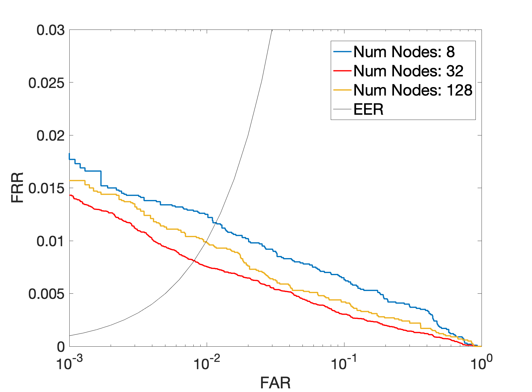
Experiments are launched on the ND-LG4000 database. The results are shown in Fig. 18 and Tab. XII. The dimensions of features are also shown in Tab. XII. The performance of 32 nodes is superior to those with 8 nodes and 128 nodes.
FG is a container of the local patterns and spatial relationships of a certain scale. If the number of nodes is insufficient, the capability of FG is not sufficient to express the local texture and spatial relationships. In contrast, if there are too many nodes, FG exhibits overfitting on the local patterns and spatial relationships in some ways.
| Num of Nodes | FRR@FAR=0.1% | EER | Feature Dimension |
|---|---|---|---|
| 8 | 1.77% | 1.17% | 512 |
| 32 | 1.43% | 0.81% | 1280 |
| 128 | 1.57% | 0.99% | 4352 |
IV-F Ablation Experiments
Ablation experiments on the graph module are conducted to evaluate the effect of the graph module in this section. In addition, ablation experiments on SE-GAT are conducted to evaluate the effects of residual structure and SE layer.
IV-F1 The Effect of the Graph Module
Two protocols are taken into consideration to evaluate the graph module: with and without the graph module. In the protocol without the graph module, all of the graph blocks are removed from the proposed framework, which makes the framework degenerate into CNNs. In the protocol with the graph module, graph blocks remain. The experiments are launched on the ND-LG4000 database, and both non-occluded and occluded instances are taken into consideration.
The results of the non-occluded instances are shown in Fig. 19 and Tab. XIII. The results of the occluded instances are shown in Fig. 20 and Tab. XIV. The performance gap between the protocols with and without the graph module is obvious, which demonstrates the effectiveness of the graph module. The gap in the case of occluded situations is larger, which indicates that the graph module is effective for occluded biometric scenarios.

| FRR@FAR=0.1% | EER | |
|---|---|---|
| without Graph | 2.27% | 1.17% |
| with Graph | 1.09% | 0.58% |

| FRR@FAR=0.1% | EER | |
|---|---|---|
| without Graph | 31.85% | 3.66% |
| with Graph | 5.09% | 1.72% |

| Residual | SE Layer | FRR@FAR=0.1% | EER | |
|---|---|---|---|---|
| Protocol A | ✓ | ✓ | 1.09% | 0.58% |
| Protocol B | ✓ | 1.35% | 0.67% | |
| Protocol C | ✓ | 2.89% | 0.95% | |
| Protocol D | 3.76% | 1.01% |
IV-F2 Ablation Study on SE-GAT
Ablation experiments on SE-GAT are conducted to evaluate the effects of residual structure and SE layer. There are four protocols: protocol A with both strategies adopted, protocol B with only a residual structure adopted, protocol C with only the SE layer adopted, and protocol D, which abandons both strategies. The results are shown in Fig. 21 and Tab. XV.
The results show that both strategies contribute to the performance of the proposed framework. The residual structure is useful to reduce the false rejection rate, which means narrowing the intraclass variance.
V Conclusion
In this paper, a novel deep learning framework called MS-DGR is proposed for handling occlusion problems in biometric recognition. The effectiveness of the proposed framework is verified on two biometric modalities, i.e. iris and face.
The proposed framework provides a novel strategy for occluded biometric recognition. Prior knowledge about the occluded region is no longer a prerequisite, and the inference is more illustrative and reasonable because of the proposed graph representation and dynamic graph matching. Different from most existing methods, the features are not selected according to mask but selected adaptively by the proposed framework. The framework is well designed for both deep learning and handcraft methods.
The main idea of this paper is straightforward, and we believe that there is much room for improvement. Further explorations of the proposed framework could focus on better methods for graph generation, multi-scale fusion, and dynamic graph matching.
Acknowledgments
The authors would like to thank the reviewers for their valuable comments and advices. This work is funded by National Natural Science Foundation of China (Grant No. 62276263, 62006225, 62071468) in part by the National Key Research and Development Program of China under Grant 2022YFC3310400, and supported by the Strategic Priority Research Program of Chinese Academy of Sciences (Grant No. XDA27040700).
References
- [1] Yann LeCun, Leon Bottou, Yoshua Bengio and Patrick Haffner, Gradient-based learning applied to document recognition, in Proceedings of the IEEE, vol. 86, no. 11, pp. 2278-2324, Nov. 1998, doi: 10.1109/5.726791.
- [2] Alex Krizhevsky, Ilya Sutskever and Geoffrey E. Hinton, ImageNet classification with deep convolutional neural networks, Advances in Neural Information Processing Systems, vol. 25, 2012.
- [3] Karen Simonyan and Andrew Zisserman, Very deep convolutional networks for large-scale image recognition, arXiv preprint arXiv:1409.1556.7923, 2014.
- [4] Christian Szegedy, Wei Liu, Yangqing Jia, Pierre Sermanet, Scott Reed, Dragomir Anguelov, Dumitru Erhan, Vincent Vanhoucke, Andrew Rabinovich, Going deeper with convolutions, Proceedings of the IEEE Conference on Computer Vision and Pattern Recognition, pp. 1-9, 2015.
- [5] Gao Huang, Zhuang Liu, Laurens van der Maaten, Kilian Q. Weinberger Densely connected convolutional networks, Proceedings of the IEEE Conference on Computer Vision and Pattern Recognition, pp. 4700-4708, 2017.
- [6] Jie Hu, Li Shen, Gang Sun, Squeeze-and-excitation networks, Proceedings of the IEEE Conference on Computer Vision and Pattern Recognition, pp. 7132-7141, 2018.
- [7] Kaiming He, Xiangyu Zhang, Shaoqing Ren and Jian Sun, Deep residual learning for image recognition, Proceedings of the IEEE Conference on Computer Vision and Pattern Recognition, pp. 770-778, 2016.
- [8] Yaniv Taigman, Ming Yang, Marc’Aurelio Ranzato and Lior Wolf, DeepFace: closing the gap to human-level performance in face verification, Proceedings of the IEEE Conference on Computer Vision and Pattern Recognition, pp. 1701-1708, 2014.
- [9] Yi Sun, Xiaogang Wang and Xiaoou Tang, Deep learning face representation from predicting 10,000 classes, Proceedings of the IEEE Conference on Computer Vision and Pattern Recognition, pp. 1891-1898, 2014.
- [10] Florian Schroff, Dmitry Kalenichenko and James Philbin, FaceNet: a unified embedding for face recognition and clustering, Proceedings of the IEEE Conference on Computer Vision and Pattern Recognition, pp. 815-823, 2015.
- [11] Weiyang Liu, Yandong Wen, Zhiding Yu, Ming Li, Bhiksha Raj and Le Song, SphereFace: deep hypersphere embedding for face recognition, Proceedings of the IEEE Conference on Computer Vision and Pattern Recognition, pp. 212-220, 2017
- [12] Jiankang Deng, Jia Guo, Niannan Xue and Stefanos Zafeiriou, ArcFace: additive angular margin loss for deep face recognition, Proceedings of the IEEE Conference on Computer Vision and Pattern Recognition, pp.4690-4699, 2019.
- [13] Ban Jozer, Matej Feder, Lubos Omelina, Oravec Milos and Jarmila Pavlovicova, Face recognition under partial occlusion and noise, Eurocon 2013, 2013, pp. 2072-2079, doi: 10.1109/EUROCON.2013.6625266.
- [14] Aisha Azeem, Meghdad Sharif, Mudassar Raza and Marryam Murtaza, A survey: face recognition techniques under partial occlusion, Int. Arab J. Inf. Technol., 2014, 11(1): 1-10.
- [15] Hao Wang, Yitong Wang, Zheng Zhou, Xing Ji, Zhifeng Li, Dihong Gong, Jingchao Zhou and Wei Liu, CosFace: large margin cosine loss for deep face recognition, Proceedings of the IEEE Conference on Computer Vision and Pattern Recognition, pp. 5265-5274, 2018.
- [16] Weihua Ou, Gai Li, Shujian Yu, Gang Xie, Fujia Ren and Yuanyan Tang, Robust discriminative nonnegative patch alignment for occluded face recognition, Springer Verlag, pp. 207-215, Nov. 2015, doi: 10.1007/978-3-319-26561-2_25.
- [17] Ismahane Cheheb, Noor Al-Maadeed, Somaya Al-madeed, Ahmed Bouridane and Richard Jiang, Random sampling for patch-based face recognition, 2017 5th International Workshop on Biometrics and Forensics (IWBF), 2017, pp. 1-5, doi: 10.1109/IWBF.2017.7935104.
- [18] Ryan Kerekes, B. Narayanaswamy, J. Thornton, M. Savvides and B. V. K. Vijaya Kumar, Graphical model approach to iris matching under deformation and occlusion, Proceedings of the IEEE Conference on Computer Vision and Pattern Recognition, pp. 1-6, 2007.
- [19] Dakshina Ranjan Kisku, Hunny Mehrotra, Phalguni Gupta and Jamuna Kanta Sing, Probabilistic graph-based feature fusion and score fusion using SIFT features for face and ear biometrics, Proc SPIE, vol. 7443, Aug. 2009, doi: 10.1117/12.824077.
- [20] Hugo Proen and Juan Briceno, Periocular biometrics: constraining the elastic graph matching algorithm to biologically plausible distortions, IET Biometrics, val. 3, Jan. 2013, doi: 10.1049/iet-bmt.2013.0039.
- [21] Kathy Horadam, Arathi Arakala, Stephen Davis and Seyed Mehdi Lajevardi, Hand vein authentication using biometric graph matching, IET Biometrics,vol. 3, Dec. 2014, doi: 10.1049/iet-bmt.2013.0086.
- [22] Ziwei Zhang, Peng Cui and Wenwu Zhu, Deep learning on graphs, arXiv preprint arXiv:1812.04202, 2018
- [23] Jie Zhou, Ganqu Cui, Zhengyan Zhang, Zhiyuan Liu, Lifeng Wang, Changcheng Li and Maosong Sun, Graph Neural Networks: a review of methods and applications, arXiv preprint arXiv: 1812.08434, 2018
- [24] Gori Marco, Monfardini Gabriele and Scarselli Franco, A new model for learning in graph domains, IEEE International Joint Conference on Neural Networks, pp. 729-734, vol. 2, Jan. 2009, doi: 10.1109/IJCNN.2005.1555942.
- [25] Franco Scarselli, Marco Gori, Ah Chung Tsoi, Markus Hagenbuchner and Gabriele Monfardini, The graph neural network model, IEEE Transactions on Neural Networks, vol. 20, no. 1, pp. 61-80, Jan. 2009, doi: 10.1109/TNN.2008.2005605.
- [26] Joan Bruna, Wojciech Zaremba, Arthur Szlam and Yann Lecun, Spectral networks and locally connected networks on graphs, arXiv preprint arXiv: 1312.6203, 2013.
- [27] Thomas N. Kipf and Max Welling, Semi-supervised classification with graph convolutional networks, arXiv preprint arXiv:1609.02907, 2016.
- [28] David Duvenaud, Dougal Maclaurin, Jorge Aguilera-Iparraguirre, Rafael Gmez-Bombarelli, Timothy Hirzel, Alan Aspuru-Guzik and Ryan P. Adams, Convolutional networks on graphs for learning molecular fingerprints, International Conference on Neural Information Processing Systems, vol. 28, 2015.
- [29] James Atwood and Don Towsley, Diffusion-convolutional neural networks, International Conference on Neural Information Processing Systems, vol. 29, 2016.
- [30] William L. Hamilton, Rex Ying and Jure Leskovec, Inductive representation learning on large graphs, International Conference on Neural Information Processing Systems, vol. 30, 2017.
- [31] Min Ren and Yunlong Wang and Zhenan Sun and Tieniu Tan, Dynamic graph representation for occlusion handling in biometrics, Proceedings of the AAAI Conference on Artificial Intelligence, vol. 34, pp. 11940-11947, 2020.
- [32] David Lowe, Object recognition from local scale-invariant features, Proceedings of the IEEE International Conference on Computer Vision, vol. 2, pp. 1150-1157, 1999.
- [33] J Long, E Shelhamer, T. Darrell, Fully convolutional networks for semantic segmentation, Proceedings of the IEEE Conference on Computer Vision and Pattern Recognition. pp. 3431-3440, 2015.
- [34] T Y Lin, P Dollor, R Girshick, et al., Feature pyramid networks for object detection, Proceedings of the IEEE Conference on Computer Vision and Pattern Recognition, pp. 2117-2125, 2017.
- [35] H Zhao and J Shi and X Qi and et al., Pyramid scene parsing network, Proceedings of the IEEE Conference on Computer Vision and Pattern Recognition, pp. 2881-2890, 2017.
- [36] Herbert Bay, Tinne Tuytelaars and Luc Van Gool, SURF: speeded up robust features, European Conference on Computer Vision. Springer, Berlin, Heidelberg, pp. 404-417, 2006.
- [37] Ira Kemelmacher and Steve Seitz and Daniel Miller and Evan Brossard, The megaface benchmark: 1 million faces for recognition at scale, Proceedings of the IEEE Conference on Computer Vision and Pattern Recognition, pp. 4873-4882, 2016.
- [38] J. G. Daugman, High confidence visual recognition of persons by a test of statistical independence, IEEE Transactions on Pattern Analysis and Machine Intelligence, vol. 15, no. 11, pp. 1148-1161, 1993.
- [39] Junlin Hu, Jiwen Lu and Yap-Peng Tan, Robust partial face recognition using instance-to-class distance, Visual Communications and Image Processing (VCIP), pp. 1-6, 2013.
- [40] Lingxiao He, Haiqing Li, Qi Zhang and Zhenan Sun, Dynamic feature learning for partial face recognition, Proceedings of the IEEE Conference on Computer Vision and Pattern Recognition, pp. 7054-7063, 2018.
- [41] Feifei Ding, Peixi Peng, Yangru Huang, Mengyue Geng and Yonghong Tian, Masked face recognition with latent part detection, Proceedings of the 28th ACM international Conference on multimedia, pp. 2281–2289, 2020.
- [42] Yande Li, Kun Guo, Yongang Lu and Li Liu, Cropping and attention based approach for masked face recognition, Applied Intelligence, vol. 51, no. 5, pp. 3012–3025, 2021.
- [43] Velikovi Petar, Cucurull Guillem, Casanova Arantxa, Romero Adriana and Bengio Yoshua, Graph attention networks, arXiv preprint arXiv:1710.10903, 2017.
- [44] Viola Paul and Jones Michael J., Robust real-time face detection, International Journal of Computer Vision, vol. 57, no. 2, pp. 137-154, 2004.
- [45] Zhaofeng He, Tieniu Tan, Zhenan Sun and Xianchao Qiu, Toward accurate and fast iris segmentation for iris biometrics, IEEE Transactions on Pattern Analysis and Machine Intelligence, vol., 31, no. 9, pp. 1670-1684, 2009.
- [46] Zhenan Sun and Tieniu Tan, Ordinal measures for iris recognition, IEEE Transactions on Pattern Analysis and Machine Intelligence, vol. 31, no. 12, pp. 2211-2226, 2009.
- [47] L. Masek, Recognition of human iris patterns for biometric identification, Master’s thesis, University of Western Australia, 2003.
- [48] Zhao Zijing and Kumar Ajay, Towards more accurate iris recognition using deeply learned spatially corresponding features, Proceedings of the IEEE International Conference on Computer Vision, pp. 3809-3818, 2017.
- [49] Zhang Qi, Li Haiqing, Sun Zhenan and Tan Tieniu, Deep feature fusion for iris and periocular biometrics on mobile devices, IEEE Transactions on Information Forensics and Security, vol. 13, no. 11, pp. 2897-2912, 2018.
- [50] Liu Nianfeng, Zhang Man, Li Haiqing, Sun Zhenan and Tan Tieniu, DeepIris: learning pairwise filter bank for heterogeneous iris verification, Pattern Recognition Letters, vol. 81, pp. 154-161, 2016.
- [51] Xiang Wu, Ran He, Sun Zhenan and Tan Tieniu, A light CNN for deep face representation with noisy labels, IEEE Transactions on Information Forensics and Security, vol. 13, no. 11, pp. 2884-2896, 2018.
- [52] Learned Miller E, Huang G B , Roychowdhury A , et al. Labeled faces in the wild: a survey Advances in Face Detection and Facial Image Analysis, Springer International Publishing, pp. 198-248, 2016.
- [53]
CASIA.V4 Iris database, (http://biometrics.idealtest.org/dbDetail
ForUser.do?id=4). - [54] ND Cross Sensor Iris 2013, (http://cvrl.nd.edu/.projects/data/#nd-crosssensor-iris-2013-data-set).
- [55] Wenjie Luo, Yujia Li, Raquel Urtasun and Richard Zemel Understanding the effective receptive field in deep convolutional neural networks, arXiv preprint arXiv:1701.04128, 2017
- [56] A. Zanfir and C. Sminchisescu, Deep learning of graph matching, Proceedings of the IEEE Conference on Computer Vision and Pattern Recognition, pp. 284-2693, 2018.
- [57] Runzhong Wang, Junchi Yan and Xiaokang Yang Learning combinatorial embedding networks for deep graph matching, Proceedings of the IEEE International Conference on Computer Vision, pp. 3056-3065, 2019.
- [58] Bo Jiang, Pengfei Sun, Jin Tang and Bin Luo Glmnet: graph learning-matching networks for feature matching, arXiv preprint arXiv:1911.07681, 2019.
- [59] Matthias Fey, Jan E. Lenssen, Christopher Morris, Jonathan Masci and Nils M. Kriege Deep graph matching consensus, arXiv preprint arXiv:2001.09621, 2020.
- [60] “Information technology biometric sample quality part 6: Iris image data, nternational Organization for Standardization, Standard ISO/IEC 29794-6:2015, 2015.
- [61] Zhongyuan Wang, Guangcheng Wang, Baojin Huang, Zhangyang Xiong, Qi Hong, Hao Wu, Peng Yi, Kui Jiang, Nanxi Wang, Yingjiao Pei, Heling Chen, Yu Miao, Zhibing Huang and Jinbi Liang Masked face recognition dataset and application, arXiv preprint arXiv:2003.09093, 2020.