Reconstructing Thermal Quantum Quench Dynamics from Pure StatesPreprint: FERMILAB-PUB-23-268-SQMS-T
Abstract
Simulating the nonequilibrium dynamics of thermal states is a fundamental problem across scales from high energy to condensed matter physics. Quantum computers may provide a way to solve this problem efficiently. Preparing a thermal state on a quantum computer is challenging, but there exist methods to circumvent this by computing a weighted sum of time-dependent matrix elements in a convenient basis. While the number of basis states can be large, in this work we show that it can be reduced by simulating only the largest density matrix elements by weight, capturing the density matrix to a specified precision. Leveraging Hamiltonian symmetries enables further reductions. This approach paves the way to more accurate thermal-state dynamics simulations on near-term quantum hardware.
I Introduction
Simulating quantum quench dynamics is a classically hard problem due to the generation of entanglement in the post-quench nonequilibrium state. It is thus a natural application for quantum computers Feynman 1982; Lloyd 1996; Miessen et al. 2023, which do not suffer from the exponential increase of resources that classical simulations experience Prosen and Žnidarič 2007. A quench is a process in which a model parameter of a quantum system changes abruptly in time, taking a stationary state into a complex superposition of excited states Barouch et al. 1970; Iglói and Rieger 2000; Sengupta et al. 2004; Barankov et al. 2004; Calabrese and Cardy 2007; Kollath et al. 2007; Moeckel and Kehrein 2008; De Grandi et al. 2010; Calabrese et al. 2011; Gagel et al. 2015; Gagel et al. 2014; Cui et al. 2019; Mitra 2018; Das 2020. Quench dynamics are of interest across physics, from cold atomic gases trapped in optical lattices Greiner et al. 2002; Kinoshita et al. 2006; Bloch et al. 2008; Bloch et al. 2012; Gring et al. 2012; Langen et al. 2015a; Nicklas et al. 2015; Langen et al. 2015b; Sun et al. 2018 to ultrafast pump-probe experiments of solid-state systems Kampfrath et al. 2013; Li et al. 2013; Matsunaga et al. 2014; Yang et al. 2018 and hadronization in heavy-ion collisions Arsene et al. 2005. Often quenches from pure states are studied, but starting from initially mixed states like thermal states is also physically interesting and experimentally relevant Prosen and Žnidarič 2007; Sotiriadis et al. 2009; Abeling and Kehrein 2016.
Quenches from pure states can be simulated naturally on quantum computers using, e.g. Suzuki-Trotter decomposition Trotter 1959; Suzuki 1976; Lloyd 1996 or variational approaches Cerezo et al. 2021; Yuan et al. 2019; Yao et al. 2021 (see Ref. Miessen et al. 2023 for a recent overview on quantum computing simulation methods for quantum dynamics). However, the evolution of mixed, thermal, or thermofield double Maldacena 2003 states encounters the challenge of preparing such states on a quantum computer Motta et al. 2020; Wu and Hsieh 2019. One means of circumventing this costly state preparation is the “evolving density matrices on qubits” (EOQ) algorithm Lamm and Lawrence 2018; Harmalkar et al. 2020; Gustafson and Lamm 2021. EOQ is a hybrid quantum-classical algorithm in which the initial density matrix in some computationally simple basis of states is obtained classically using a stochastic method such as density matrix quantum Monte Carlo (DMQMC) Blunt et al. 2014 or Euclidean lattice field theory. The quantum dynamics simulations are then performed with corresponding basis states which can be more easily prepared, and the convolution with the classically obtained reconstructs the full mixed-state dynamics.
While EOQ is an appealing hybrid algorithm, it potentially requires a unique quantum simulation for all elements of to reconstruct the dynamics. However, often it may be unnecessary to evolve all initial states; e.g., in gapped systems at a low temperature, only a limited set of configurations may be required. Further, one can truncate to reduce the number of quantum simulations to at the price of systematically-improvable errors.
Here we study the effect of truncation on the simulated dynamics of thermal states. We investigate the structure of thermal and simulate the dynamics of such states with varying . Optimizations of the truncation approximation are investigated, such as choosing appropriate bases for depending on the model parameters and the observables measured. Another optimization is to exploit symmetry relations between basis states to reduce the number of unique simulations required. In doing so, we demonstrate that can be reduced by up to two orders of magnitude from the naive estimate. We apply our techniques to quenches from thermal states in the mixed-field Ising model, using both exact diagonalization (ED) and DMQMC to prepare . While our study is inspired by quantum computing as a promising use case, we carry it out on classical computers as we are addressing questions of principle rather than implementation. The latter direction is a logical next step for future work, and we briefly comment further on it in our conclusion.
The remainder of the paper is organized as follows. First, we briefly review the EOQ and DMQMC algorithms in Sec. II. In Sec. III, the mixed-field Ising model and the quench protocol are defined. Sec. IV is devoted to the impact of truncating . This is followed by Sec. V where symmetries are used to further reduce . Classical dynamics simulations are presented in Sec. VI to demonstrate how accuracy depends on the truncation. We consider one system size where is easily accessible by ED, and another where full ED becomes expensive and DMQMC becomes a desirable algorithmic choice. Sec. VII concludes and describes future steps.
II EOQ algorithm
Ultimately, our goal is to compute the expectation value of an observable at a time . In the Heisenberg picture, the time evolution of with a Hamiltonian is given by . Our initial state is defined via a Hamiltonian by and has an inverse temperature . Then, the expectation value is
| (1) |
where we have resolved the trace in a complete basis.
The EOQ algorithm of Ref. Lamm and Lawrence 2018 reconstructs the dynamics in Eq. (1) by first classically obtaining a stochastic approximation and the matrix elements using DMQMC Blunt et al. 2014. With a stochastic algorithm like DMQMC, it is possible to reach larger system sizes than ED. The un-normalized thermal is approximated through DMQMC by a stochastic solution to the symmetric Bloch equation
| (2) |
with the initial condition Lamm and Lawrence 2018. This stochastic solution is obtained in DMQMC by discretizing . Then one initializes a number of imaginary particles called “psips” in the diagonal states . At each step, these psips are allowed to move in the space of basis states with probabilistic rules derived from Eq. (2). Note that each psip also carries a sign, so that its contribution to a given density matrix element can be positive or negative. From this, is obtained as a sum over psips:
| (3) |
where is determined by the number and sign of the psips associated with and ensures normalization. (We note that are taken in this work to be real.) The finiteness of naturally truncates since any matrix element with will be zero. The statistical error of is derived from Poisson statistics in Appendix A. This error can be systematically reduced by including more psips in DMQMC.
With the classical simulation (using either DMQMC or ED) designating which are nonzero, the quantum computer is used to obtain the matrix elements . Combining these with produces an approximation to Eq. (1). To obtain the matrix elements , one initializes the quantum computer in the superposition states
| (4) | ||||
and evaluates the time-dependence of via
| (5) | ||||
(We discuss the contribution of state preparation to the quantum simulation overhead in Appendix C.) Note that in many cases, is purely real. In any case, naively a number of quantum dynamics simulations is required to perfectly reconstruct the dynamics of a of size .
The goal of this work is to investigate whether can be further reduced by judicious truncation of and by leveraging symmetries. To address this question, we use classical simulations to obtain either itself by ED or by DMQMC. While the former approach only works for relatively small systems, it allows for faithful benchmarking against the exact dynamics.
III Model and quench protocol

In this section we discuss the one-dimensional antiferromagnetic mixed-field Ising model (MFIM) and the specific quench protocol used in our simulations. The MFIM Hamiltonian is
| (6) |
and includes a nearest-neighbor antiferromagnetic (AFM) Ising coupling and transverse and longitudinal fields and . We also include a small staggered magnetic field to weakly lift the degeneracy of the ground state in the AFM phase. We assume periodic boundary conditions such that , and hereafter set as a unit of energy and inverse time. We restrict to even for convenience.
At and , the model exhibits AFM and paramagnetic (PM) phases separated by a continuous phase transition except at , where the model reduces to the classical Ising model and exhibits a first-order transition at . The order parameter for the AFM phase is the staggered magnetization density
| (7) |
In the disordered PM phase, as long as the ground state acquires finite magnetization density
| (8) |
The phase diagram is found in Fig. 1a) as determined by density matrix renormalization group (DMRG) simulations in Ref. Ovchinnikov et al. 2003.
Although no ordered phase exists when , for sufficiently small , has high weight on the Néel state for parameters belonging to the zero-temperature AFM phase. Since the initial sets an energy scale below which states contribute significantly to , increasing results in more energy eigenstates contributing to , as shown in Fig. 1b). Similarly, more states contribute to near the critical point , where the energy gap approaches its minimum. Thus, the structure of depends on parameters of the model and initial state, as we discuss in Sec. IV.
In our simulations, and are given by the MFIM Hamiltonian (6) with different choices of couplings. is defined by the couplings , while the quench Hamiltonian is defined by couplings and with . Physically, this corresponds to an abrupt parameter quench in which the fields are changed: , , and . Eq. (6) is nonintegrable for Kim et al. 2014; Prosen and Žnidarič 2007. We consider three quenches to the point , starting from the initial points and . These quenches are represented by arrows in Fig. 1a).
IV Structure and Truncation of

To reduce the simulation cost of evaluating Eq. (1), we now investigate how to systematically omit some while retaining a certain accuracy. As mentioned in Sec. I, we expect that certain parameter regimes of should be less sensitive to discarding specific . For example, in the AFM phase at large , has high weight on only a few : specifically, if is represented in the -basis, the Néel states and should dominate over all other configurations. Similarly, if the initial state is deep in the PM phase, a single spin-polarized configuration should dominate. In contrast, for initial states close to the phase boundary—where the energy gap scales as —or at small , we expect many large .
To make this intuition quantitative, we consider a truncated density matrix with nonzero elements as a function of and couplings. is defined via a set of indices , with for all (note that ). The cutoff is chosen such that the weight , defined via the ratio of Frobenius norms
| (9) |
is above a fixed threshold. Note that we normalize the truncated density matrix .
In Fig. 2, we calculate the required to achieve as a function of and system size for each quench with . Since this quantity depends on the basis in which is represented, we show results for both the - and -basis. Focusing first on the -basis results, there is a clear trend of increasing with increasing . This is due to the fact that the initial state becomes polarized in the -basis for large , and therefore can only be represented using all -basis states. For example, in the extreme limit and , becomes fully dense, involving all matrix elements in the -basis. Remnants of this behavior are clearly visible for the larger values in Fig. 2c) (), where the required approaches . As decreases, becomes more diagonal, so that at only matrix elements are nonzero. This effect is also visible in the curve in Fig. 2c). Meanwhile, in the AFM phase at [Fig. 2a)], we see that far fewer -basis matrix elements are required, especially at large . However, in all phases we observe the general tendency that increases exponentially with .
The -basis results mirror the -basis results. In the AFM phase [Fig. 2d), ], where the density matrix is sparser in the -basis, the -basis representation of is much denser. In contrast, the density matrix sparsens in the PM phase [Fig. 2f), ], especially at high . Finally, we observe that near the quantum critical point [Fig. 2b) and e), ] the difference in between different basis representations is greatly reduced, especially at low . This is consistent with the intuition that more density matrix elements should be required in any basis near the phase transition due to the pileup of eigenstates at low energies.
V Leveraging Symmetries
In general, and are constrained by symmetries of the Hamiltonians and . Here we discuss how to leverage these to further reduce .
The symmetries of [Eq. (6)] impose a degeneracy structure on . has a two-site translation symmetry owing to the presence of ; we denote the generator of this symmetry by . Additionally, when the model is invariant under the global spin-flip . This operation commutes with the and terms in but anticommutes with the staggered field. However, the latter also anticommutes with bond-centered reflection , which maps site to site when is even, and one-site translation , both of which commute with the remainder of . Thus, the combined operations , , and are symmetries for . The impact of these symmetries on the structure of can be seen as follows. Given a unitary operator that commutes with , any satisfies
| (10) |
where and . Thus, given in any basis, one immediately knows . Since and , we can obtain from any at most additional elements. This is particularly useful when using DMQMC, which does not a priori preserve the symmetries of . By demanding that symmetry-related are identical, we can produce a symmetrized DMQMC estimate .
The symmetries of , namely and , can also be used to reduce . The effect of these symmetry transformations on depends on the choice of observable . For example, for the symmetry generators commute with both the and the and we then obtain an expression analogous to Eq. (10) with replaced by . When , and anticommute with the observable but commute with . We therefore find, for a general element of the symmetry group (where and ) 11 1 We note in passing that the group generated by and is isomorphic to , the dihedral group with elements. This follows from and the fact that . The latter equation can be checked by computing the action of both sides on a general computational basis element. These properties can be used to show that a general group element can be written in the form ., that
| (11) |
where now and . Thus, from a single simulation yielding the matrix element , we can obtain at most additional between symmetry-related basis states at no cost.

Finally, we note that Eq. (V) can be used to eliminate certain simulations entirely. In particular, if we are interested in between eigenstates of , we can apply Eq. (V) with to observe that, since and when and are eigenstates, we must have that for those states. This allows us to explicitly exclude from Eq. (1), corresponding to the upper triangle of the matrix in the space of reflection-symmetric states. Furthermore, since commutes with and anticommutes with , we have that
| (12) |
When and are -eigenstates, these . This increases the number of excluded states by a multiplicative factor of at most .
In summary, symmetries relate both and . When transforms simply under the symmetry group of (e.g. if it is invariant or acquires a minus sign), a single yields a family of matrix elements related by symmetry at no additional simulation cost. Furthermore, when anticommutes with a symmetry generator (e.g. ), minus signs appear which can be used to additionally exclude matrix elements between any two eigenstates of that generator. Furthermore, and are always Hermitian, so one need only consider upper-triangular matrix elements of both operators. Combining all of these simplifications allows us to reduce , as we will demonstrate below.
VI Simulation Results
We now present the results of classical simulations of thermal quench dynamics for the observables and . We focus on two example systems, in Sec. VI.1 a chain of length sites, and in Sec. VI.2 a chain of length . In the former case, exact numerical results are accessible via ED, so that detailed benchmarking can be performed as a function of . In the latter case, full ED is impractical but DMQMC simulations can yield an accurate estimate of to simulate the in Eq. (1). In this case, attention must be paid to the impact of the systematic error in the DMQMC algorithm on the subsequent dynamics.
VI.1 -site Chain (ED Initial State)
For chains, can be obtained from via ED. An exact simulation of the dynamics of an operator can then be obtained directly by computing the Heisenberg operator where is obtained by direct matrix exponentiation using eigenstates of . The late-time steady state value of can be calulated via the thermal diagonal ensemble (TDE) average of . This TDE average is defined by analogy with the diagonal ensemble (DE) average Rigol et al. 2008 in pure state dynamics as
| (13) |
where and are eigenvalues labeling eigenstates of and , respectively. The TDE average can be viewed as a Boltzmann-weighted average of the DE value of for pure-state quenches from every eigenstate of . We will say that the system has equilibrated when the time-average of reaches the TDE value.
In Fig. 3, we compare the exact result for to results obtained by evaluating Eq. (1) using . To calculate the contribution of the matrix elements to the dynamics, we perform simulations to obtain the corresponding matrix elements . [We count as one simulation, although multiple simulations may be required using the superposition states (4).] Many are related by symmetry, so , often much less. In Fig. 3, we explore how varying affects accuracy.

The observable dynamics in Fig. 3 is indicative of the initial and final locations of the quench. If the quench begins in the AFM phase [panels a)–c) and d)–f)] we use and perform dynamics simulations in the -basis; if it begins in the PM phase [panels g)–i)] we use and simulate in the -basis. Correlating the sampling basis with the observable in this way minimizes the needed to capture the expectation value at time . The TDE average of the observable, which indicates the late-time value of , is observed to be nonzero only for quenches within the PM region (). For [panels a)–c)], increasing generally results in larger captured for a fixed . This matches the expectation based on Fig. 2a), where the largest- required the smallest . For [panels d)–f)], the initial state is at the quantum critical point, but evidently retains some residual AFM order at finite size. In this case, a larger is required to capture the dynamics as compared to the results. Nevertheless, we still observe the general trend that increasing increases the captured by a fixed . Finally, for [panels g)–i)], we can only exclude simulations based on the smaller set of symmetries of . However, even after accounting for symmetries, we observe that needs to be about an order of magnitude larger to capture the dynamics than for . This is likely due to the fact that the spins polarize in the - plane rather than purely along the axis when . Nevertheless, we observe in all cases that exploiting symmetries reduces by one to two orders of magnitude compared to .
VI.2 -site Chain (DMQMC Initial State)
We simulate thermal quench dynamics for using DMQMC to obtain [see Eq. (3)] for parameters . The approximate initial value clearly approaches this DMQMC value as a function of . Additionally, we see oscillations about as expected for a quench from the quantum critical point into the PM phase, which suggests that the dynamics have equilibrated. These results further demonstrate the utility of symmetries, which allow .
The curves in Fig. 4 are shown with confidence bands indicating how the statistical uncertainty from finite in propagates into the dynamics calculation. The detailed derivation of this error propagation is presented in Appendix A. We note that the uncertainty is time-dependent due to variations in the relative contributions of the as derived in Eq. (16). Of particular note is that the statistical error in the dynamics scales down with increasing .
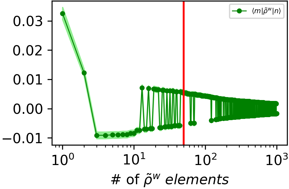
The dynamics plots in Fig. 4 are calculated using truncated density matrices capturing a weight of at most of . To understand why such a small weight might be sufficient, Fig. 5 shows for the first matrix elements sorted by magnitude from highest to lowest. We see that the matrix elements rapidly become very small, however care must be taken since their smallness can in principle be counteracted by their exponentially large number. Nevertheless, we also observe that, as the density matrix elements become smaller in magnitude, they begin to oscillate in sign and therefore contribute incoherently to Eq. (1). Indeed, such oscillations become more likely as the density matrix elements become smaller and the statistics noisier. (This is an example of a sign problem in Monte Carlo analysis.) This sign incoherence motivates our choice of a relatively small in our simulations and suggests that the simulation cost may scale favorably as a function of .
VII Discussion and Outlook
The EOQ algorithm Lamm and Lawrence 2018 provides an approach to simulating quench dynamics from a thermal initial state using a combination of classical and quantum techniques. The initial step of thermal state preparation is circumvented using a classical stochastic algorithm, while the classically hard task of time evolution is carried out on a quantum computer. The desired operator dynamics is then reconstructed by a weighted average of the basis state dynamics results. A crucial shortcoming of this approach is that, generically, the needed to reconstruct the thermal quench dynamics grows exponentially with system size. In this work we have investigated the possibility of mitigating this issue by systematically truncating the initial density matrix. We have also shown that symmetries can be exploited to further reduce the number of dynamics simulations needed to account for a fixed number of density matrix elements.
The efficacy of the methods developed here depends strongly on the initial temperature and Hamiltonian parameters. For example, at low initial temperature and for initial Hamiltonian parameters for which the zero-temperature ground state is gapped, we find that the thermal quench dynamics of certain operators can be reconstructed from only a handful of pure state dynamics simulations [see Fig. 3c) and i)]. However, at high temperatures or for initial Hamiltonian parameters that correspond to a zero-temperature quantum critical point, substantially more dynamics simulations are required. Regardless of the parameters of the initial state, we find that leveraging symmetries allows for a reduction by one to two orders of magnitude in the number of pure state dynamics simulations needed to capture the contribution from a fixed number of density matrix elements. Although these techniques do not eliminate the exponential scaling issue, we expect that they will be indispensable for future implementations of EOQ at system sizes comparable to or beyond those accessible to ED.
One challenge worth addressing in future work is the difficulty of quantifying the influence of density matrix truncation error on the dynamics of observables. In this work, we probed the effect of truncation on the dynamics by changing , but it would be desirable to have an estimate of the statistical uncertainty in a dynamical expectation value due to truncation. This would allow one to estimate, from results with a fixed , a confidence band around the simulated time trace of the observable. Such an understanding would become increasingly valuable as the simulations are scaled up to larger system sizes, to the point where the “exact” dynamics from the DMQMC initial state is no longer simulable, like in the case of discussed above. With access to exact dynamics, it is possible to calculate truncation error. Fig. 6 shows the complicated convergence of the truncation error defined as
| (14) |
with increasing weight and for . The at fixed (see, e.g., the points corresponding to ) is largest for ,where more states contribute significantly to the dynamics.

A number of future applications of the techniques developed here can be envisioned. One example is the calculation of thermal Green’s functions, which hinge on calculating quantities of the form . Here the initial state and time evolution are defined with respect to the same Hamiltonian , unlike the thermal quench protocols considered here. Nevertheless, the same density matrix truncation and symmetry approaches considered here could readily be applied. We also note that pure-state two-time correlation functions can be simulated on quantum computers with only constant overhead Mitarai and Fujii 2019. Another direction is to apply these methods to the simulation of dynamical phase transitions Heyl et al. 2013; Heyl 2018, which have also been studied in the context of mixed-state dynamics Bhattacharya et al. 2017; Heyl and Budich 2017. It would be interesting to consider the fate of the zero-temperature dynamical phase transition Heyl et al. 2013 when the initial state is at finite . Simulating such phenomena requires calculating the Loschmidt echo, which can be achieved on quantum computers using Hadamard-test protocols Ortiz et al. 2001; Somma et al. 2002 or ancilla-free versions thereof Mitarai and Fujii 2019. It may also be possible to incorporate some of the techniques considered here into classical tensor network algorithms for calculating finite temperature properties, such as the minimally entangled typical thermal states method Stoudenmire and White 2010; Binder and Barthel 2017; Bruognolo et al. 2015.
Acknowledgements.
This material is based on work supported by the U.S. Department of Energy, Office of Science, National Quantum Information Science Research Centers, Superconducting Quantum Materials and Systems Center (SQMS) under contract number DE-AC02-07CH11359. Fermilab is operated by Fermi Research Alliance, LLC under contract number DE-AC02-07CH11359 with the United States Department of Energy. T.I. acknowledges the Aspen Center for Physics, which is supported by National Science Foundation grant PHY-2210452, where part of this work was performed. P.P.O. thanks A. Vishwanath and Harvard University for hospitality during the final stages of this project.Appendix A Statistical error
For a function with variables , the error is given by . Consider . Here
| (15) |
where where is the set of non-zero matrix elements of (see Sec. IV; recall that in practice we take to be real.). All three, and are square and symmetric. We write where is the number of psips corresponding to the matrix element and is the sign of the corresponding element, determined by the net charge of the psips. We also define the number of diagonal psips, . Poisson statistics implies that . The error in the dynamics of the observable is given by
| (16) |
When , the error in is
| (17) |
When , the error in is
| (18) |
Appendix B Calculation of observable matrix elements
Here we discuss two ways to calculate the time-dependent matrix elements on a quantum computer. For , the calculation is straightforwardly accomplished by a direct measurement of following the dynamics under from the initial pure state . For , and noticing that it is easier to compute diagonal expectation values than off-diagonal overlaps where , we can perform time-evolution starting from and defined in Eq. (4). Efficient quantum circuits to prepare these states are discussed in the next Section C. Computing the four diagonal expectation values yields
| (19) | ||||
| (20) |
If is Hermitian, i.e. , both expectation values are real:
| (21) | ||||
| (22) |
Eq. (5) follows directly from the above.
Another method to measure off-diagonal matrix elements of observables is the Hadamard test Ortiz et al. 2001; Somma et al. 2002, whose circuit is shown in Fig. 7. The Hadamard test can be applied to measure off-diagonal elements of a unitary operator . We can use it to measure by expanding the Hermitian operator in the Pauli basis, where are Pauli strings. If and are related by , where is the set of sites where the computational basis states and differ, then we can write
| (23) |
We can define and in Fig. 7 and then sum over to obtain the desired result. The Hadamard test is unwieldy because it requires a controlled- gate controlled by an ancilla qubit. As an alternative to the Hadamard test, one can also explore protocols like the ones proposed in Ref. Mitarai and Fujii 2019 that avoid the need for an ancilla-controlled gate at the expense of running more direct measurement circuits. Whether such methods are more desirable than that of preparing the superposition states (4) is hardware-dependent.
Appendix C Initial superposition state preparation
Here we consider the quantum resource cost of preparing the superposition states (4) on a quantum computer. Preparing such states requires at most CNOT gates: indeed, for and , the states (4) are variants of the GHZ state Greenberger et al. 1989. More generally, the complexity of state-preparation is highest for superpositions of states satisfying , i.e. ones that differ on all sites. The circuit depth needed to prepare such states can be reduced in certain cases by parallelizing the CNOT gates: Ref. Cruz et al. 2019 found that the circuit depth can be reduced to assuming sufficient qubit connectivity and a system size that is a power of two. A general example of such a circuit for is shown in Fig. 8. The superposition states and for which are indexed by -gate powers , . determines whether the state is of type or , determines the sign, and the remainder dictate the pattern of bits in each state. For example, setting all in Fig. 8 gives the GHZ state while setting gives the GHZ-like states . Fewer CNOT gates are required for and that differ on fewer sites. For a general off-diagonal element, and differ on at least one qubit. Applying a Hadamard gate to one of these qubits, followed by a set of appropriately parallelized CNOTs, generates the desired superposition. An example circuit is shown in Fig. 9.
Appendix D Thermal diagonal ensemble
We use the following expression for the TDE [],
| (24) | ||||
where the sum is performed over and are eigenstates of and respectively. Taking the infinite-time limit in analogy with Eq. (2) from Rigol et al. 2008, i.e., assuming attenuation of the off-diagonal terms due to temporal dephasing, we find
| (25) |
In the infinite-temperature limit,
| (26) |
as expected. In the zero-temperature limit,
| (27) |
in analogy with Eq. (2) from Rigol et al. 2008. This corresponds to a pure-state quench from , the ground state of .
References
- Feynman (1982) R. P. Feynman, Simulating physics with computers, Int. J. Theor. Phys. 21, 467 (1982).
- Lloyd (1996) S. Lloyd, Universal quantum simulators, Science 273, 1073 (1996).
- Miessen et al. (2023) A. Miessen, P. J. Ollitrault, F. Tacchino, and I. Tavernelli, Quantum algorithms for quantum dynamics, Nat Comput Sci 3, 25 (2023).
- Prosen and Žnidarič (2007) T. Prosen and M. Žnidarič, Is the efficiency of classical simulations of quantum dynamics related to integrability?, Phys. Rev. E 75, 015202 (2007).
- Barouch et al. (1970) E. Barouch, B. M. McCoy, and M. Dresden, Statistical Mechanics of the XY Model. I, Phys. Rev. A 2, 1075 (1970).
- Iglói and Rieger (2000) F. Iglói and H. Rieger, Long-Range Correlations in the Nonequilibrium Quantum Relaxation of a Spin Chain, Phys. Rev. Lett. 85, 3233 (2000).
- Sengupta et al. (2004) K. Sengupta, S. Powell, and S. Sachdev, Quench dynamics across quantum critical points, Phys. Rev. A 69, 053616 (2004).
- Barankov et al. (2004) R. A. Barankov, L. S. Levitov, and B. Z. Spivak, Collective Rabi Oscillations and Solitons in a Time-Dependent BCS Pairing Problem, Phys. Rev. Lett. 93, 160401 (2004).
- Calabrese and Cardy (2007) P. Calabrese and J. Cardy, Quantum quenches in extended systems, J. Stat. Mech. 2007, P06008 (2007).
- Kollath et al. (2007) C. Kollath, A. M. Läuchli, and E. Altman, Quench Dynamics and Nonequilibrium Phase Diagram of the Bose-Hubbard Model, Phys. Rev. Lett. 98, 180601 (2007).
- Moeckel and Kehrein (2008) M. Moeckel and S. Kehrein, Interaction Quench in the Hubbard Model, Phys. Rev. Lett. 100, 175702 (2008).
- De Grandi et al. (2010) C. De Grandi, V. Gritsev, and A. Polkovnikov, Quench dynamics near a quantum critical point, Phys. Rev. B 81, 012303 (2010).
- Calabrese et al. (2011) P. Calabrese, F. H. L. Essler, and M. Fagotti, Quantum quench in the transverse-field ising chain, Phys. Rev. Lett. 106, 227203 (2011).
- Gagel et al. (2015) P. Gagel, P. P. Orth, and J. Schmalian, Universal postquench coarsening and aging at a quantum critical point, Phys. Rev. B 92, 115121 (2015).
- Gagel et al. (2014) P. Gagel, P. P. Orth, and J. Schmalian, Universal postquench prethermalization at a quantum critical point, Phys. Rev. Lett. 113, 220401 (2014).
- Cui et al. (2019) T. Cui, M. Schütt, P. P. Orth, and R. M. Fernandes, Postquench gap dynamics of two-band superconductors, Phys. Rev. B 100, 144513 (2019).
- Mitra (2018) A. Mitra, Quantum quench dynamics, Annual Review of Condensed Matter Physics 9, 10.1146/annurev-conmatphys-031016-025451 (2018).
- Das (2020) S. R. Das, Quantum quench and universal scaling, Oxford University Press and the American Institute of Physics 10.1093/acrefore/9780190871994.013.55 (2020).
- Greiner et al. (2002) M. Greiner, O. Mandel, T. Esslinger, T. W. Hänsch, and I. Bloch, Quantum phase transition from a superfluid to a mott insulator in a gas of ultracold atoms, Nature 415, 39 (2002).
- Kinoshita et al. (2006) T. Kinoshita, T. Wenger, and D. S. Weiss, A quantum newton’s cradle, Nature 440, 900 (2006).
- Bloch et al. (2008) I. Bloch, J. Dalibard, and W. Zwerger, Many-body physics with ultracold gases, Rev. Mod. Phys. 80, 885 (2008).
- Bloch et al. (2012) I. Bloch, J. Dalibard, and S. Nascimbene, Quantum simulations with ultracold quantum gases, Nature Physics 8, 267 (2012).
- Gring et al. (2012) M. Gring, M. Kuhnert, T. Langen, T. Kitagawa, B. Rauer, M. Schreitl, I. Mazets, D. A. Smith, E. Demler, and J. Schmiedmayer, Relaxation and Prethermalization in an Isolated Quantum System, Science 337, 1318 (2012).
- Langen et al. (2015a) T. Langen, S. Erne, R. Geiger, B. Rauer, T. Schweigler, M. Kuhnert, W. Rohringer, I. E. Mazets, T. Gasenzer, and J. Schmiedmayer, Experimental observation of a generalized Gibbs ensemble, Science 348, 207 (2015a).
- Nicklas et al. (2015) E. Nicklas, M. Karl, M. Höfer, A. Johnson, W. Muessel, H. Strobel, J. Tomkovič, T. Gasenzer, and M. K. Oberthaler, Observation of Scaling in the Dynamics of a Strongly Quenched Quantum Gas, Phys. Rev. Lett. 115, 245301 (2015).
- Langen et al. (2015b) T. Langen, R. Geiger, and J. Schmiedmayer, Ultracold Atoms Out of Equilibrium, Annual Review of Condensed Matter Physics 6, 201 (2015b).
- Sun et al. (2018) W. Sun, C.-R. Yi, B.-Z. Wang, W.-W. Zhang, B. C. Sanders, X.-T. Xu, Z.-Y. Wang, J. Schmiedmayer, Y. Deng, X.-J. Liu, S. Chen, and J.-W. Pan, Uncover topology by quantum quench dynamics, Phys. Rev. Lett. 121, 250403 (2018).
- Kampfrath et al. (2013) T. Kampfrath, K. Tanaka, and K. A. Nelson, Resonant and nonresonant control over matter and light by intense terahertz transients, Nature Photon 7, 680 (2013).
- Li et al. (2013) T. Li, A. Patz, L. Mouchliadis, J. Yan, T. A. Lograsso, I. E. Perakis, and J. Wang, Femtosecond switching of magnetism via strongly correlated spin–charge quantum excitations, Nature 496, 69–73 (2013).
- Matsunaga et al. (2014) R. Matsunaga, N. Tsuji, H. Fujita, A. Sugioka, K. Makise, Y. Uzawa, H. Terai, Z. Wang, H. Aoki, and R. Shimano, Light-induced collective pseudospin precession resonating with Higgs mode in a superconductor, Science 345, 1145 (2014).
- Yang et al. (2018) X. Yang, C. Vaswani, C. Sundahl, M. Mootz, P. Gagel, L. Luo, J. H. Kang, P. P. Orth, I. E. Perakis, C. B. Eom, and J. Wang, Terahertz-light quantum tuning of a metastable emergent phase hidden by superconductivity, Nature Mater 17, 586 (2018).
- Arsene et al. (2005) I. Arsene et al., Quark–gluon plasma and color glass condensate at rhic? the perspective from the brahms experiment, Nuclear Physics A 757, 1 (2005), first Three Years of Operation of RHIC.
- Sotiriadis et al. (2009) S. Sotiriadis, P. Calabrese, and J. Cardy, Quantum quench from a thermal initial state, EPL (Europhysics Letters) 87, 20002 (2009).
- Abeling and Kehrein (2016) N. O. Abeling and S. Kehrein, Quantum quench dynamics in the transverse field ising model at nonzero temperatures, Phys. Rev. B 93, 104302 (2016).
- Trotter (1959) H. F. Trotter, On the product of semi-groups of operators, Proceedings of the American Mathematical Society 10, 545 (1959).
- Suzuki (1976) M. Suzuki, Generalized trotter's formula and systematic approximants of exponential operators and inner derivations with applications to many-body problems, Communications in Mathematical Physics 51, 183 (1976).
- Cerezo et al. (2021) M. Cerezo, A. Arrasmith, R. Babbush, S. C. Benjamin, S. Endo, K. Fujii, J. R. McClean, K. Mitarai, X. Yuan, L. Cincio, and P. J. Coles, Variational quantum algorithms, Nature Reviews Physics 3, 10.1038/s42254-021-00348-9 (2021).
- Yuan et al. (2019) X. Yuan, S. Endo, Q. Zhao, Y. Li, and S. C. Benjamin, Theory of variational quantum simulation, Quantum 3, 191 (2019).
- Yao et al. (2021) Y.-X. Yao, N. Gomes, F. Zhang, C.-Z. Wang, K.-M. Ho, T. Iadecola, and P. P. Orth, Adaptive variational quantum dynamics simulations, PRX Quantum 2, 030307 (2021).
- Maldacena (2003) J. Maldacena, Eternal black holes in anti-de sitter, Journal of High Energy Physics 2003, 021 (2003).
- Motta et al. (2020) M. Motta, C. Sun, A. T. K. Tan, M. J. O’Rourke, E. Ye, A. J. Minnich, F. G. S. L. Brandão, and G. K.-L. Chan, Determining eigenstates and thermal states on a quantum computer using quantum imaginary time evolution, Nature Physics 16, 10.1038/s41567-019-0704-4 (2020).
- Wu and Hsieh (2019) J. Wu and T. Hsieh, Variational thermal quantum simulation via thermofield double states, Physical Review Letters 123 (2019).
- Lamm and Lawrence (2018) H. Lamm and S. Lawrence, Simulation of Nonequilibrium Dynamics on a Quantum Computer, Phys. Rev. Lett. 121, 170501 (2018), arXiv:1806.06649 [quant-ph] .
- Harmalkar et al. (2020) S. Harmalkar, H. Lamm, and S. Lawrence (NuQS), Quantum Simulation of Field Theories Without State Preparation (2020), arXiv:2001.11490 [hep-lat] .
- Gustafson and Lamm (2021) E. J. Gustafson and H. Lamm, Toward quantum simulations of gauge theory without state preparation, Phys. Rev. D 103, 054507 (2021), arXiv:2011.11677 [hep-lat] .
- Blunt et al. (2014) N. S. Blunt, T. W. Rogers, J. S. Spencer, and W. M. C. Foulkes, Density-matrix quantum monte carlo method, Phys. Rev. B 89, 245124 (2014).
- Ovchinnikov et al. (2003) A. A. Ovchinnikov, D. V. Dmitriev, and V. O. Cheranovskii, Antiferromagnetic ising chain in a mixed transverse and longitudinal magnetic field, Phys. Rev. B 68, 10.1103/PhysRevB.68.214406 (2003).
- Kim et al. (2014) H. Kim, T. N. Ikeda, and D. A. Huse, Testing whether all eigenstates obey the eigenstate thermalization hypothesis, Phys. Rev. E 90, 052105 (2014).
- (49) We note in passing that the group generated by and is isomorphic to , the dihedral group with elements. This follows from and the fact that . The latter equation can be checked by computing the action of both sides on a general computational basis element. These properties can be used to show that a general group element can be written in the form .
- Rigol et al. (2008) M. Rigol, V. Dunjko, and M. Olshanii, Thermalization and its mechanism for generic isolated quantum systems, Nature 452, 10.1038/nature06838 (2008).
- Mitarai and Fujii (2019) K. Mitarai and K. Fujii, Methodology for replacing indirect measurements with direct measurements, Phys. Rev. Res. 1, 013006 (2019).
- Heyl et al. (2013) M. Heyl, A. Polkovnikov, and S. Kehrein, Dynamical quantum phase transitions in the transverse-field ising model, Physical Review Letters 110, 10.1103/physrevlett.110.135704 (2013).
- Heyl (2018) M. Heyl, Dynamical quantum phase transitions: a review, Reports on Progress in Physics 81, 054001 (2018).
- Bhattacharya et al. (2017) U. Bhattacharya, S. Bandyopadhyay, and A. Dutta, Mixed state dynamical quantum phase transitions, Phys. Rev. B 96, 180303 (2017).
- Heyl and Budich (2017) M. Heyl and J. C. Budich, Dynamical topological quantum phase transitions for mixed states, Phys. Rev. B 96, 180304 (2017).
- Ortiz et al. (2001) G. Ortiz, J. E. Gubernatis, E. Knill, and R. Laflamme, Quantum algorithms for fermionic simulations, Phys. Rev. A 64, 022319 (2001).
- Somma et al. (2002) R. Somma, G. Ortiz, J. E. Gubernatis, E. Knill, and R. Laflamme, Simulating physical phenomena by quantum networks, Phys. Rev. A 65, 042323 (2002).
- Stoudenmire and White (2010) E. M. Stoudenmire and S. R. White, Minimally entangled typical thermal state algorithms, New Journal of Physics 12, 055026 (2010).
- Binder and Barthel (2017) M. Binder and T. Barthel, Symmetric minimally entangled typical thermal states for canonical and grand-canonical ensembles, Phys. Rev. B 95, 195148 (2017).
- Bruognolo et al. (2015) B. Bruognolo, J. von Delft, and A. Weichselbaum, Symmetric minimally entangled typical thermal states, Phys. Rev. B 92, 115105 (2015).
- Cruz et al. (2019) D. Cruz, R. Fournier, F. Gremion, A. Jeannerot, K. Komagata, T. Tosic, J. Thiesbrummel, C. L. Chan, N. Macris, M.-A. Dupertuis, and C. Javerzac-Galy, Efficient quantum algorithms for ghz and w states, and implementation on the ibm quantum computer, Advanced Quantum Technologies 2, 10.1002/qute.201900015 (2019).
- Greenberger et al. (1989) D. M. Greenberger, M. A. Horne, and A. Zeilinger, Going beyond bell’s theorem, in Bell’s theorem, quantum theory and conceptions of the universe (Springer, 1989) pp. 69–72.