The bulk Euclidean saddle point geometry $X$ preparing the cosmological state of interest is built by gluing two patches of thermal AdS spaces (generically at different temperatures) along the worldvolume of a thin shell of pressureless matter, as illustrated in Fig. 1. In this regard, our construction is reminiscent of the construction in ref. [66] of two-sided black hole microstates with long Einstein-Rosen bridges. In order for $X$ to be dominant over the competing black hole solution, we require the inverse temperatures $\tilde{\beta}_{\mathsf{L}},\tilde{\beta}_{\mathsf{R}}$¹¹ 1 The inverse temperatures $\tilde{\beta}_{\mathsf{L}},\tilde{\beta}_{\mathsf{R}}$ represent the Euclidean preparation time of the CFT microstate. The corresponding physical inverse temperatures $\beta_{\mathsf{L}},\beta_{\mathsf{R}}$ of the left and right Euclidean AdS spaces are given by the sum of the preparation temperatures and the Euclidean time elapsed by the shell’s trajectory, see eq. (2.14). to be large in units of the AdS radius $\ell$. In other words, we are interested in studying the gravitational system below its characteristic Hawking-Page temperature.

In this regime, the time reflection-symmetric slice $\Sigma$ of $X$, on which the the bulk semiclassical state is prepared, contains three connected components, $\Sigma=\Sigma_{\mathsf{l}}\cup\Sigma_{\mathsf{c}}\cup\Sigma_{\mathsf{r}}$. Each of the two components $\Sigma_{\mathsf{l}}$ and $\Sigma_{\mathsf{r}}$ corresponds to a hyperbolic disk, providing the initial data of two independent AdS spacetimes (AdS_l and AdS_r). The last component, $\Sigma_{\mathsf{c}}$, is a closed universe of spherical topology. It is formed by two hyperbolic disks $\Sigma_{\mathsf{c}_{\mathsf{l}}},\Sigma_{\mathsf{c}_{\mathsf{r}}}$ with a radial cut off at $r=R_{*}$ (which is equal for the two components), glued together along the position of the thin shell. The causal development of the initial data on $\Sigma_{\mathsf{c}}$, denoted by $\mathsf{c}=\mathsf{c}_{\mathsf{l}}\cup\mathsf{c}_{\mathsf{r}}$, consists of two patches of global AdS, glued along the spherical worldvolume of the thin shell. The shell collapses towards the past and the future, generating the big bang and big crunch singularities of the cosmological spacetime $\mathsf{c}$.

More concretely, the metric on each one of the two AdS patches forming the cosmology can be locally characterized by the open FLRW metric

where $\text{d}\mathbf{H}_{d}^{2}=\text{d}\rho^{2}+\sinh^{2}\rho\,\text{d}\Omega_{d-1}^{2}$ is the hyperbolic metric of a FLRW slice. In this form, the metric is homogeneous and isotropic, with the scale factor given by $a(t_{c})=\ell\cos(t_c/\ell)$. The singularities arising at $t_{c}=\pm\pi\ell/2$ are only coordinate singularities. In fact, this metric covers a hyperbolic slicing of a Wheeler-DeWitt (WDW) patch of a pure AdS spacetime.

However, $\mathsf{c}_{\mathsf{l}}$ and $\mathsf{c}_{\mathsf{r}}$ are strictly contained within the WDW patch covered by the metric (1.1) and they become truly singular due to the presence of the collapsing shell. We will show in Sec. 2 that each FLRW time slice of $\mathsf{c}_{\mathsf{l}}$ and $\mathsf{c}_{\mathsf{r}}$ is cut off at the location of the shell, implicitly given by $\rho=\rho_{\max}(t_{c})$, where $\rho_{\max}(t_{c})$ parametrizes the radial trajectory of the shell in these coordinates (see Fig. 7). In particular, the size of the spatial slices shrinks to zero at $t_{c}=\pm t_{f}$, with $t_{f}<\pi\ell/2$, corresponding to the endpoints of the shell’s collapse. The spacetime curvature is singular at these points, which we identify with the big bang and the big crunch singularities of our cosmological spacetime.²² 2 The geometry of $\mathsf{c}_{\mathsf{l}}$ and $\mathsf{c}_{\mathsf{r}}$ is similar to the one arising inside a collapsing shell of matter during black hole formation. The future singularity of our cosmological spacetime can then be identified with the black hole singularity. Unlike usual black hole formation setups, our construction is time reversal-symmetric and there is a past singularity as well.

$\mathsf{c}_{\mathsf{l}}$ and $\mathsf{c}_{\mathsf{r}}$ can then be understood to be two patches of a closed,³³ 3 Although the spatial FLRW slices of each patch $\mathsf{c}_{\mathsf{l}}$ and $\mathsf{c}_{\mathsf{r}}$ are hyperbolic, each spatial slice is cut off at the location of the shell and glued to another identical portion of a spatial slice, giving rise to a closed cosmology. $\Lambda<0$, big bang-big crunch cosmology. Although this cosmology looks homogeneous and isotropic locally (i.e. within the $\mathsf{c}_{\mathsf{l}}$ and $\mathsf{c}_{\mathsf{r}}$ patches), it is actually inhomogeneous due to the presence of the shell. In particular, the cosmological singularities are inhomogeneous: they do not arises from the scale factor vanishing in each patch, but rather from the size of the spatial slices shrinking to zero due to the collapse of the shell of matter.

The classical solutions built this way provide sensible (macroscopic) cosmologies if the shell is heavy, of rest mass $m\ell\gg 1$. As we will explain, this regime can be approached microscopically, by taking the large-$N$ limit of the holographic CFT, and considering that the dual operator to the thin shell is heavy, with a conformal dimension scaling with $N^{2}$. Additionally, we will be alluding to the case of a very heavy shell throughout this paper, treated formally in the $m\ell\rightarrow\infty$ limit. In this parametric regime, many of the calculations that we will encounter simplify considerably. Of course, we expect that this limit provides a good approximation to very large but finite $m\ell$ as well.

A clear example where such simplification occurs is at the level of the entanglement structure of the state of the quantum fields on $\Sigma$, in the bulk effective field theory (EFT). Specifically, the path integral of the bulk fields on $X$ prepares a specific bulk EFT state, via a bulk time-dependent Hamiltonian coupling all of the three components of $\Sigma$. At intermediate values of $m\ell$, the bulk state prepared this way generally shares entanglement between the three connected components of $\Sigma$. In the limit of large mass for the shell, however, the shell’s worldvolume $\mathcal{W}$ effectively pinches off in Fig. 1. This drastically reduces the coupling between the two sides of the cosmology $\Sigma_{\mathsf{c}_{\mathsf{l}}},\Sigma_{\mathsf{c}_{\mathsf{r}}}\subset\Sigma_{\mathsf{c}}$, in the Euclidean preparation. As a result, the bulk state prepared by $X$ will contain mostly bipartite entanglement between each side of the cosmology ($\Sigma_{\mathsf{c}_{\mathsf{l}}},\Sigma_{\mathsf{c}_{\mathsf{r}}}$), and the respective AdS region ($\Sigma_{\mathsf{l}},\Sigma_{\mathsf{r}}$). Moreover, in this case, the bulk state prepared by $X$ roughly correspond to two bulk thermofield doubles, at temperatures $\beta_{\mathsf{L}}$ (for AdS_l and $\mathsf{c}_{\mathsf{l}}$) and $\beta_{\mathsf{R}}$ (for AdS_r and $\mathsf{c}_{\mathsf{r}}$), with fields in the cosmology purifying fields in the AdS regions.

Given the construction of the Euclidean geometry $X$ preparing the bulk state, it is natural (and convenient for the reasons described in Sec. 2) to consider more general bulk states on $\Sigma$, with additional entanglement between the AdS regions and the cosmology. Such states can be easily prepared with the addition of local operator insertions along the Euclidean preparation manifold $X$ (see Sec. 2.2). For similar reasons, in the large mass limit for the thin shell, all of the bulk states prepared in this way contain mostly bipartite entanglement.

The gravitational path integral preparing the cosmological state holographically corresponds to the Euclidean CFT path integral on flat cylinders of lengths $\tilde{\beta}_{\mathsf{L}}/2$ and $\tilde{\beta}_{\mathsf{R}}/2$, with the insertion of a heavy operator $\mathcal{O}$ dual to the shell in between these Euclidean evolutions (see Fig. 4). This path integral prepares a so-called partially entangled thermal state (PETS) of two independent copies of the holographic CFT,

where each CFT lives on a spatial $\mathbf{S}^{d-1}$ of radius $\ell$. The two-point function of the operator $Z_{1}=\text{Tr}(e^{-\tilde{\beta}_{\mathsf{L}}H}\mathcal{O}^{\dagger}e^{-\tilde{\beta}_{\mathsf{R}}H}\mathcal{O})$ normalizes the state.

The insertion of the heavy CFT operator $\mathcal{O}$ in the path integral provides the boundary condition for the worldvolume of the thin shell at the asymptotic boundary of the Euclidean geometry $X$. The specific operator corresponding to the thin shell is $\mathcal{O}\sim\prod_{i}\mathcal{O}_{\Delta}(\Omega_{i})$, formed by a large number of single trace operator insertions $\mathcal{O}_{\Delta}(\Omega_{i})$, of low conformal dimension $\Delta\ll N^{2}$, distributed in an approximately homogeneous way along the sphere, $\Omega_{i}\in\mathbf{S}^{d-1}$. In what follows, we consider that the number of operator insertions is $O(N^{2})$, which implies that the associated bulk backreaction cannot be treated perturbatively in the $1/N$ expansion. Still, the matrix elements of the shell operator $\mathcal{O}$ admit an effective gaussian description in the energy basis, at least at the level of the two-point function, given that the shell effectively behaves as a spherical heavy particle (see [67]).

In the absence of any operator insertion (i.e. when $\mathcal{O}=\mathbb{1}$), the PETS becomes a low-temperature TFD state of two independent CFTs in the confined phase, dual to a pair of AdS spacetimes with bulk quantum fields entangled between the two components to form a bulk thermofield-double state. The insertion of the heavy thin shell operator causes the non-perturbative modification of the semiclassical state, leading to the presence of the closed cosmology in the way described above. Similarly, in the high temperature regime, i.e. above the associated confinement/deconfinement phase transition temperature for the state, the semiclassical description of the PETS becomes that one of the two-sided black hole microstates constructed in ref. [66], where the black hole contains a large interior geometry, supported by the presence of the shell.

The construction of these cosmological states admitting a holographic dual description should be regarded as the first main result of the present paper.

Given the construction of the cosmological microstates described above, in Sec. 3 we derive, through a standard gravitational replica trick calculation, that the entanglement entropy of the reduced state $\rho_{\mathsf{L}}$ to the CFT_L follows a version of the quantum-corrected RT formula. We denote by $\rho_{i}$, $i=\mathsf{l},\mathsf{r},\mathsf{c}$, the density matrices for the bulk quantum fields restricted on the time symmetric slices of the two AdS regions $\Sigma_{\mathsf{l}}$, $\Sigma_{\mathsf{r}}$ and of the cosmology $\Sigma_{\mathsf{c}}$, respectively. The global state on the bulk Cauchy slice $\Sigma=\Sigma_{\mathsf{l}}\cup\Sigma_{\mathsf{c}}\cup\Sigma_{\mathsf{r}}$ is pure, i.e. $S(\rho_{\mathsf{l}\mathsf{c}\mathsf{r}})=0$.

In the present setup, the entropy of the bulk fields is $O(G^{0})$ and therefore subleading with respect to any ${O}(G^{-1})$ area term. This implies that all possible geometrically non-empty extremal surfaces are disfavored and that the RT surface is indeed empty, $\gamma_{\mathsf{L}}=\emptyset$, for the CFT_L.⁴⁴ 4 An interesting classical extremal surface is given by the initial sphere associated to the position of the shell, at $r=R_{*}$, in the time reflection-symmetric slice $\Sigma$. This surface has index 1 at least, which means that the surface is maximal in at least one direction of deformation space, as opposed to the candidate RT surfaces, which are always minimal surfaces. In the regime where the quantum-corrected RT prescription is valid, the whole cosmology resembles a python’s lunch, encoded in either CFT_L or CFT_R. However, due to the presence of the closed cosmology, it is still necessary to specify the homology hypersurface $\Sigma_{\mathsf{L}}$, with $\partial\Sigma_{\mathsf{L}}=\mathsf{L}$. The two possibilities are:

• •

  The homology hypersurface is $\Sigma_{\mathsf{L}}=\Sigma_{\mathsf{l}}$, and it does not include the cosmology. The bulk entanglement entropy of $\rho_{\Sigma_{\mathsf{L}}}$ given by this candidate is $S(\rho_{\mathsf{l}})$.

• •

  The homology hypersurface is $\Sigma_{\mathsf{L}}=\Sigma_{\mathsf{l}}\cup\Sigma_{\mathsf{c}}$, which includes the full closed cosmology. The bulk entanglement entropy of $\rho_{\Sigma_{\mathsf{L}}}$ given by this candidate is $S(\rho_{\mathsf{l}\mathsf{c}})=S(\rho_{\mathsf{r}})$.

From these considerations, the naive application of the quantum-corrected RT prescription leads to the island formula

This results suggests that whenever $S(\rho_{\mathsf{l}\mathsf{c}})<S(\rho_{\mathsf{l}})$—i.e. whenever the entanglement between AdS_l and $\mathsf{c}_{\mathsf{l}}$ is larger than the entanglement between AdS_r and $\mathsf{c}_{\mathsf{r}}$, given that $S(\rho_{\mathsf{l}\mathsf{c}})=S(\rho_{\mathsf{r}})$—the entanglement wedge of CFT_L will contain the cosmology $\mathsf{c}$. If, on the contrary, $S(\rho_{\mathsf{r}})>S(\rho_{\mathsf{l}})$, the cosmology will be contained in the entanglement wedge of CFT_R. See Fig. 2 for a visual representation of the former case.

We would like to remark that the situation is more subtle. The derivation of the minimization prescription of eq. (1.3) requires that one of the two terms dominates over the other, with corrections which are negligible when $\exp(|S(\rho_{\lef})- S(\rho_{\ri})|)\gg 1$. This condition is generally satisfied by the excited cosmological states we will be interested in even if the bulk entropies $S(\rho_{\mathsf{r}})$ and $S(\rho_{\mathsf{l}})$ are in general $O(N^{0})$ in the large-$N$ expansion, as we will explain in Sec. 2.2. If, however, the two terms become comparable or if both terms are small, then we cannot consider the cosmology to be encoded in any one of the two CFTs, but only in the union of both CFTs. For example, this is the case for the simple PETS state below the Hawking-Page temperature (1.2), for which $S(\rho_{\mathsf{l}})$ and $S(\rho_{\mathsf{r}})$ are generically small in string theory constructions of AdS/CFT (see Appendix B), as well as in any bottom-up model, unless a parametrically large number of bulk species is added by hand.

In Sec. 3, we derive the island formula (1.3) from Euclidean gravity, adopting the FLM replica trick prescription of refs. [7, 9] for these particular cosmological microstates. In this case, different saddle point geometries arise from different thin shell contractions between replicated CFT contours. These provide different contributions to the Rényi entropies of $\rho_{\mathsf{L}}$, which in the end leads to (1.3) upon analytic continuation. In particular, the island term, $S(\rho_{\mathsf{l}\mathsf{c}})$, originates from a “replica wormhole” saddle point geometry with thin shell contractions between different boundary replicas. This phenomenon was first noticed in a different context in the “west coast model” of black hole evaporation [18]. An important aspect of the present replica trick calculation is that the classical contribution of every saddle point geometry contributing to the Rényi entropies factors out, and cancels with the semiclassical normalization of the state $\rho_{\mathsf{L}}$. The remaining non-trivial contributions arise from suitable one-loop partition functions of the bulk fields on top of each geometry, leading to eq. (1.3).

The construction of the cosmological microstates sets the stage for an interesting question: how is the cosmological EFT encoded holographically in the CFTs? We address this question in Sec. 4 by studying the bulk-to-boundary map between the bulk EFT and the microscopic dual CFTs. The encoding of the bulk EFT on the AdS_l and AdS_r spacetimes into the CFT_L and CFT_R, respectively, presents no difficulty and is given in terms of the standard AdS/CFT dictionary. Therefore, we are particularly interested in understanding the trickier question of how different bulk states in the cosmology $\mathsf{c}$ are mapped to CFT states, and how to reconstruct the action of bulk operators on $\mathsf{c}$ from the dual boundary theory.

For this reason, we focus our attention on the bulk Hilbert space $\mathcal{H}_{\psi}\subset\mathcal{H}_{\Sigma}$ obtained by acting on a reference state $\ket{\psi}\in\mathcal{H}_{\Sigma}$ with local unitary operators supported only on the time-symmetric slice of the cosmology $\Sigma_{\mathsf{c}}$, where $\mathcal{H}_{\Sigma}$ is the full bulk EFT Hilbert space defined on the time reflection-symmetric slice $\Sigma=\Sigma_{\mathsf{l}}\cup\Sigma_{\mathsf{c}}\cup\Sigma_{\mathsf{r}}$. In other words, we fix the state $\rho_{\mathsf{l}\mathsf{r}}$ and thus the bulk entanglement entropy between the AdS regions and the cosmology, and consider different bulk states by acting on the cosmological degrees of freedom (DOF). In this paper we will refer to the bulk theory restricted to this class of states as the “cosmological EFT”. We call the resulting bulk-to-boundary map $V_{\psi}:\mathcal{H}_{\psi}\rightarrow\mathcal{H}_{\mathsf{L}}\otimes\mathcal{H}_{\mathsf{R}}$ (with $\mathcal{H}_{\mathsf{L},\mathsf{R}}$ Hilbert spaces of the left and right CFTs) the cosmology-to-boundary map.⁵⁵ 5 Note that we will discuss the global cosmology-to-boundary map. Some of our results apply to the single-sided cosmology-to-boundary map given by entanglement wedge reconstruction, when the cosmology is encoded in only one of the two CFTs, i.e. when the island formula (1.3) holds.

In order to simplify our analysis, we restrict our attention to operator insertions $\phi_{i}$ at the time reflection-symmetric slice in the cosmology that create localized particles on top of some reference bulk state $\ket{\psi}$. These particles are heavy (i.e. $m_{i}\ell\gg 1$), but light enough that their backreaction on the geometry can be neglected. The resulting bulk states have the form

where $z_{I}$ is a normalization factor and $y_{i}\in\Sigma_{\mathsf{c}}$. The condition $m_{i}\ell\gg 1$ guarantees that we can use the geodesic approximation in the Euclidean geometry to relate the operator insertions in the cosmology to corresponding local CFT operator insertions—which we will collectively represent by $\mathbb{O}_{I}(\mathbf{x}_{I})$—in the Euclidean path integral preparing the reference state $\ket{\Psi}=V_{\psi}\ket{\psi}$ (see Fig. 14):

where $\mathcal{T}$ denotes Euclidean time ordering, the operator $\mathcal{O}(\tilde{\beta}_{\mathsf{R}}/2)$ inserts the shell, and we collectively represented by $\mathcal{O}_{\Psi}(\mathbf{x}_{\Psi})$ the operator insertions in the Euclidean path integral preparing the reference state $\ket{\Psi}$.

Given this simple class of bulk states and their dual boundary states, we can investigate the properties of the cosmology-to-boundary map $V_{\psi}$ relating the two. The first result that we derive in Sec. 4.1 is that $V_{\psi}$ is non-isometric. To show this, we consider two orthogonal bulk states $\ket{\psi_{I_i}}$, $\ket{\psi_{I_j}}$ with different configurations of particles in the cosmology. In the bulk EFT, $\bra{\psi_{I_i}}\ket{\psi_{I_j}}=0$ by assumption.⁶⁶ 6 We consider states with particles in the cosmology carrying different internal DOF, so that the bulk overlap vanishes up to $1/N$-suppressed corrections due to gravitational interactions between the particles. The CFT overlap of the dual states, $G_{ij}=\bra{\Psi_{I_i}}\ket{\Psi_{I_j}}=\bra{\psi_{I_i}}V_{\psi}^{\dagger}V_{\psi}\ket{\psi_{I_j}}$, is however non-vanishing. Computing it semiclassically requires to use the bulk Euclidean gravitational path integral. The connected CFT overlap vanishes, $\overline{G_{ij}}=0$, where the overline indicates that we evaluated the quantity within the semiclassical gravity approximation. The square of the overlap, $\overline{|G_{ij}|^{2}}$, is however non-vanishing in this approximation, due to the contribution coming from an Euclidean wormhole saddle point geometry (see Fig. 16). In the large mass limit, the contribution of this overlap becomes universal, independent of the details of $\ket{\psi_{I_i}}$ and $\ket{\psi_{I_j}}$. It is given by

where $S_{2}(\rho_{\mathsf{l},\mathsf{r}})$ is the second Rényi entropy of the bulk state $\rho_{\mathsf{l},\mathsf{r}}$ of the AdS_l,r region, respectively. Note that, as we have discussed above, $S_{2}(\rho_{\mathsf{l},\mathsf{r}})\sim O(N^{0})$ and therefore the square of the overlap is not parametrically suppressed in the large-$N$ limit. However, for general excited reference states $\ket{\psi}$ of the bulk EFT, with a large amount of entanglement between the cosmology and the AdS regions, the overlap is small.

This calculation signals that in general the CFT overlap $G_{ij}$ is non-vanishing. The bulk EFT only reproduces the average value of the CFT overlap, whose structure is pseudo-random and depends on microscopic details of the states. It however cannot capture deviations from it, even if these contributions are not parametrically suppressed in $\exp(-N^2)$, see Sec. 4.1 for additional details. Remarkably, the bulk Euclidean path integral is nonetheless able to reproduce some structure of these deviations, once Euclidean wormhole saddles are allowed when computing the moments. From this perspective, we can conclude that the map $V_{\psi}$ is non-isometric (i.e. $V^{\dagger}_{\psi}V_{\psi}\neq\mathbb{1}$) since it does not preserve the inner product structure of the cosmological EFT.

We want to emphasize that the non-isometricity of the cosmology-to-boundary map does not imply that such a map is non-invertible. This would only be the case in finite-dimensional toy models of $V_{\psi}$, where a clear “bag of gold paradox” arises [68, 69, 18]. In AdS/CFT, however, the boundary description has an infinite dimensional Hilbert space, and we generally expect that orthogonal states in the bulk EFT are mapped to non-orthogonal but still linearly-independent states in the dual boundary theory, so that $V_{\psi}^{-1}$ exists.⁷⁷ 7 We thank Mark Van Raamsdonk for discussions on this point. The information distinguishing all of the bulk states is in principle stored on thermal tails of the CFT wavefunction of these states (see Sec. 4.2 for additional details on this point). In this way, all of the bulk EFT states can at least in principle be distinguished by a boundary observer, provided that this observer can probe the CFT states to an arbitrary accuracy.

On the other hand, for CFT observers with finite resolution, such as those only sensitive to a specific microcanonical band, a bag of gold paradox does arise. Under this restriction, we show in Sec. 4.2 that the universal overlap (1.6) and its higher moments are consistent with the fact that the cosmology-to-boundary map, restricted to a microcanonical window, has a non-trivial kernel and is therefore non-invertible. Intuitively, ignoring the information contained in thermal tails of the microscopic states, and restricting to a CFT microcanonical window, null states appear and many of the cosmological states look linearly dependent as an artifact of this truncation. We further show that the overlap (1.6) and its higher moments are consistent with the low-energy microcanonical density of states of the CFTs. By choosing a number of bulk EFT orthogonal states $K>e^{\textbf{S}}$ (where $\textbf{S}=S_{\mathsf{l}}+S_{\mathsf{r}}$ with $S_{\mathsf{l},\mathsf{r}}$ bulk microcanonical entropies in AdS_l,r) the dual CFT microstates span the microcanonical window.

Finally, in Sec. 4.3, we turn our attention to the reconstruction of bulk operators acting on the cosmology. Consider a bulk operator $\phi(y)$ acting on a bulk state $\ket{\psi_I}$ and creating a particle at a point $y\in\Sigma_{\mathsf{c}}$ in the cosmology, and the corresponding boundary operator $\Phi=V_{\psi}\phi V_{\psi}^{-1}$ acting on the CFT state $\ket{\Psi}$. In standard AdS/CFT, the bulk operator $\phi$ is dual to a given CFT generalized free field $\mathcal{O}_{\phi}$ which is identified by means of the extrapolate dictionary. One then writes down a smeared version of the generalized free field, with an appropriate kernel, which provides the HKLL representation of the local bulk operator in the CFT [70, 71]. In the case of the cosmology, any causal reconstruction is doomed to fail, since the cosmology $\mathsf{c}$ is geometrically disconnected from the asymptotic boundaries where the dual theory is defined.

In order to obtain an explicit reconstruction of the bulk operator, we can use the fact that the state $\Phi\ket{\Psi_I}=V_{\psi}\phi(y)\ket{\psi_I}$ can be prepared by a Euclidean path integral of the form (1.5) with the addition of an extra operator insertion $\mathcal{O}_{\phi}$ at a specific Euclidean time $\tau_{\phi}$.⁸⁸ 8 For a generic bulk operator $\phi$ with small mass, the corresponding CFT operator insertion in the Euclidean path integral is non-local. We will again restrict for simplicity to the case of operators that can be treated under the geodesic worldline approximation, for which a local insertion of $\phi$ in the bulk corresponds to a local insertion of $\mathcal{O}_{\phi}$ in the Euclidean boundary. The matrix elements of the CFT operator $\Phi$ then take the form

In this expression, the Euclidean time ordering $\mathcal{T}$ of the CFT operator insertions is crucial for the correct definition of the matrix elements. Since different bulk states correspond to insertions of different operators $\mathcal{O}_{\Psi},\mathbb{O}_{I}$ at different Euclidean times $\tau_{\Psi},\tau_{I}$, the right-hand-side of eq. (1.7) depends on the states $\ket{\Psi_I}$ and $\ket{\Psi_J}$, and the matrix elements of the CFT operator $\Phi$ need to be defined one by one. In this sense, the explicit Euclidean reconstruction (1.7) of the bulk operators acting on the cosmology is manifestly state-dependent.

The properties of the cosmology-to-boundary map $V_{\psi}$ outlined above and the state-dependent reconstruction of the cosmological EFT operators described above should be regarded as the second main result of the present paper.

In order to study the properties of the cosmology-to-boundary map more explicitly, we introduce a tensor network (TN) toy model for the cosmological states that qualitatively captures all of the properties of the AdS/CFT setup described above, see Fig. 3.

In this TN, described in detail in Sec. 5, the triangles on the left and right represent MERA TNs modeling the initial slices of the AdS_l,r spacetimes; the triangles with a curved edge are MERAs cut off at $r=R_{*}$ which represent the $\mathsf{c}_{\mathsf{l},\mathsf{r}}$ initial slices; the projection labeled by $\mathcal{O}$ glues the two cosmological MERAs together and has the interpreation of the shell operator $\mathcal{O}$; the lines labeled by $|\mathsf{l}|=2^{S_{\mathsf{l}}},|\mathsf{r}|=2^{S_{\mathsf{r}}}$ represent the EPR pairs between the AdS_l,r regions and the cosmology; the lines labeled by $|\mathsf{c}_{\mathsf{l},\mathsf{r}}|$ represent bulk DOF on the cosmology, including those entangled with AdS_l,r and additional, DOF which are not entangled; finally, the box labeled by $\psi_{i}$ represents a bulk state $\ket{\psi_i}$ on $\Sigma=\Sigma_{\mathsf{l}}\cup\Sigma_{\mathsf{c}}\cup\Sigma_{\mathsf{r}}$. We can tune the entanglement between the AdS_l,r spaces and the cosmological components $\mathsf{c}_{\mathsf{l},\mathsf{r}}$, by increasing the number of EPR pairs by hand, given by the parameters $S_{\mathsf{l},\mathsf{r}}$ of the TN. Note that the state $\ket{\psi}$ is a state defined on all of the bulk DOF, and in particular also on the AdS_l,r DOF which are not entangled with the cosmology (which we did not represent here for simplicity, given that they are irrelevant for our discussion).

Moreover, we choose the tensor $\mathcal{O}$ to be Gaussian random, with zero mean and unit variance.⁹⁹ 9 This assumption is motivated by the coarse-grained semiclassical description of the thin shell operator $\mathcal{O}$ in terms of a Gaussian random matrix in the energy basis [67]. With this choice, a TN replica trick calculation shows that this random TN approximately saturates the RT formula on the TN, which is the analog of the island formula (1.3) described above for the AdS/CFT setup. Interestingly, the island term in the TN replica trick arises from a replica-connected contribution present when taking averages over the $\mathcal{O}$ tensor, in analogy with the gravitational replica wormhole contribution in AdS/CFT.

Given the TN of Fig. 3, we consider general states $\ket{\psi_i}$ of the cosmological EFT, that is, those states generated by acting on a reference state $\ket{\psi}$ with local unitaries $U_{\mathsf{c}}^{(i)}$ supported on the DOF of the cosmology. The TN in Fig. 3 defines a cosmology-to-boundary map

where $\bra{\Pi_{\Op}}_{\mathsf{c}}=\bra{\Op}I_{\mathsf{c}_{\mathsf{l}}}I_{\mathsf{c}_{\mathsf{r}}}$ is the “cosmological projector” associated with the random shell tensor and the $I_{\mathsf{c}_{\mathsf{l},\mathsf{r}}}$ cutoff MERA isometries, $I_{\mathsf{l},\mathsf{r}}$ are the AdS MERA isometries, and $\Pi^{i}_{\text{MAX}}=\ket{\text{MAX}_i}\bra{\text{MAX}_i}$ is the orthogonal projector to the maximally entangled state of $S_{\mathsf{l},\mathsf{r}}$ pairs between AdS_l,r and $\mathsf{c}_{\mathsf{l},\mathsf{r}}$, respectively.

In general, the dimension of the Hilbert space of cosmological DOF can be larger than the entanglement between the cosmology and the AdS regions, i.e. $|\mathsf{c}_{\mathsf{l}}||\mathsf{c}_{\mathsf{r}}|>|\mathsf{l}||\mathsf{r}|$. Since the TN defines a linear map between finite-dimensional Hilbert spaces, this implies that, in this regime, there are null states in the cosmological EFT, i.e. $\text{dim}\{\text{Ker}(V_{\psi})\}=|\mathsf{c}_{\mathsf{l}}||\mathsf{c}_{\mathsf{r}}|-|\mathsf{l}||\mathsf{r}|>0$, and the map $V_{\psi}$ is non-isometric. Thus, unlike the previous discussion in AdS/CFT, the TN model of the cosmology-to-boundary map in this case has a non-trivial kernel. This is a consequence of the finite dimensional nature of the TN, in which high energy states have been projected out and thus the information contained on thermal tails (which in principle enables to distinguish different cosmological states in the CFT) is lost. The TN should be regarded as a model of what a CFT observer with finite resolution can distinguish, in analogy with the situation described above in which we truncate the CFT Hilbert space by projecting onto a microcanonical band of the CFT.

By exploiting the gaussian isoperimetric inequalities for the random $\mathcal{O}$ tensor, we can estimate under which condition the map $V_{\psi}$ is approximately isometric for all states that a computationally limited bulk observer can prepare (both the notion of approximate isometry and the definition of these “simple” states are made precise in Sec. 5.2) with extremely high probability. We find that this is the case if

where $|\mathsf{c}|=|\mathsf{c}_{\mathsf{l}}||\mathsf{c}_{\mathsf{r}}|$ and $q$ is a constant given in eq. (5.28). This result shows that in order to have an approximately isometric encoding of all “simple” cosmological states, it is enough that the number of entangled pairs $S_{\mathsf{l}}+S_{\mathsf{r}}$ between cosmology and AdS regions scales logarithmically with the number of DOF in the cosmology.

We expect that these considerations to also hold under genericity assumptions for the full-fledged cosmology-to-boundary map in AdS/CFT. A simple estimate of the cosmological dimension in this case is $\log_{2}|\mathsf{c}|\sim 2N^{p}$, for $p<2$, associated to the microcanonical entropy of two gases of particles in AdS, one on each of the patches $\mathsf{c}_{\mathsf{l}}$ and $\mathsf{c}_{\mathsf{r}}$. The regime (1.9) is still within the microcanonical stability of the gas of particles in AdS, and it can therefore be attained in our construction.

The non-isometric to approximately isometric transition for the cosmology-to-boundary map, when the entanglement to the cosmology exceeds the bound (1.9), should be regarded as the third main result of the present paper.

The rest of the paper is organized as follows. In Sec. 2 we present a detailed construction of the cosmological states in the bulk and boundary theories and describe the properties of the cosmological spacetime. In Sec. 3 we derive the island formula from the FLM replica trick calculation for these states. In Sec. 4 we analyze the properties of the cosmology-to-boundary map restricted to specific states prepared via the insertion of localized matter operators in the CFT Euclidean path integral, and provide an explicit state-dependent reconstruction of operators acting on the cosmology. In Sec. 5 we present a TN toy model of our setup and analyze generic properties of the cosmology-to-boundary map using this model. We end with a discussion of our results in Sec. 6. Technical details related to our results can be found in Appendices A-E.

In the EFT (2.2), the shell propagates freely at tree level, following a codimension-one worldvolume $\mathcal{W}$ which bisects the Euclidean geometry $X$ into two components $X_{\pm}$. To leading order, we shall neglect the backreaction exerted by the state of the quantum fields on $X$. At this level, the metric on $X_{\pm}$ will be that of thermal AdS

where

Each Euclidean time coordinate is periodic with periodicity given by the physical inverse temperature of the corresponding AdS space, $\tau_{-}\sim\tau_{-}+\beta_{\mathsf{L}}$ and $\tau_{+}\sim\tau_{+}+\beta_{\mathsf{R}}$. The radial coordinate must remain continuous across the gluing of these two solutions across $\mathcal{W}$, given that it measures the proper areas of transverse spheres. It therefore has the same label for both components in (2.3).

From spherical symmetry of $\mathcal{W}$, the embedding functions of $\mathcal{W}$ in $X_{\pm}$ reduce to $\tau_{\pm}=\tau_{\pm}(T)$ and $r=R(T)$, where $T$ is the thin shell’s proper Euclidean time, and $R(T)$ is its radial trajectory. The rest of the angular coordinates over $\mathbf{S}^{d-1}$ are inherited from the metrics (2.3). The induced metric on $\mathcal{W}$ is simply

The gluing of $X_{\pm}$ is performed solving Einstein’s field equations locally in a neighbourhood of $\mathcal{W}$. This leads to the so-called Israel-Darmois junction conditions [82, 83]. The first condition states that the metric should remain continuous along $\mathcal{W}$, which, from (2.3) and (2.5), translates to

where the dot represents $\frac{\text{d}}{\text{d}T}$. The second junction condition quantifies how the normal derivative of the induced metric jumps across $\mathcal{W}$. The total jump is given by the energy-momentum tensor of the thin shell, which from (A.4) has dust form, $T_{\mu\nu}|_{\mathcal{W}}=\sigma u_{\mu}u_{\nu}$, for $u_{\mu}=(\text{d}T)_{\mu}$ the proper velocity of each particle forming the shell. Combined with (2.6) this condition yields (see e.g. [84])

In this expression we have introduced the total rest mass of the shell

where $V_{\Omega}=\text{Vol}(\mathbf{S}^{d-1})$. The total rest mass $m$ is conserved by virtue of the angular components of the second junction condition. It correspond to an intrinsic property which characterizes the shell operator used in the construction of the state.¹²¹² 12 In the microscopic description of the shell, given by the CFT operator $\mathcal{O}$, the parameter $m$ is related to the total conformal dimension $m\sim\Delta_{\mathcal{O}}\sim n\Delta$, where $n\sim N^{2}$ is the number of local operator insertions that form $\mathcal{O}$, each of conformal dimension $\Delta$.

Squaring (2.7) produces the equation of motion of a non-relativistic particle with zero total energy, moving in one dimension,

which describes the radial motion of the thin shell. The effective potential is

The second term of the effective potential corresponds to the gravitational self-energy of the shell, which creates a repulsive force in the Euclidean section. This makes the shell bounce at a given radius $R_{*}>0$, satisfying $V_{\text{eff}}(R_{*})=0$.¹³¹³ 13 Setups similar to those described in this paper cannot be achieved using holographic BCFT constructions dual to spacetimes containing end-of-the-world (ETW) branes like in [85, 86, 45, 46, 51, 52]. In fact, at least in these minimal models, the brane’s equation of state is that of constant proper energy density (its stress-energy tensor is proportional to the induced metric), leading to a brane’s trajectory without turning points when the background is pure AdS: the brane simply shrinks from $r=\infty$ to $r=0$ in Euclidean signature. Therefore, the insertion of two branes at symmetric Euclidean times leads to two disconnected ETW branes (see [45] for an explicit construction), and the corresponding Lorentzian manifold does not contain a disconnected component (the cosmology) like in the present setup. The shell’s trajectory then starts from the Euclidean asymptotic boundary at $R=\infty$, dives into the bulk until it turns around at $R=R_{*}$, and then goes back to $R=\infty$ again (see Fig. 1).¹⁴¹⁴ 14 For $d=2$, these solutions only exist for $R_{*}>0$ if $2Gm>1$. In higher dimensions, they always exist.

The turning radius $R_{*}$ is a function of the shell’s mass, $R_{*}=R_{*}(m)$. For large mass in AdS units, $m\ell\gg 1$, the turning radius scales as

measured in units of the $(d+1)$-dimensional Planck length $\ell_{P}=G^{\frac{1}{d-1}}$. The classical solution can thus be trusted if the shell is parametrically heavy in AdS units. In this case, its mass density $\sigma$ remains parametrically smaller than the Planck density along $\mathcal{W}$.

The total Euclidean time elapsed by the shell from the point of view of each component $X_{\pm}$ can be obtained by plugging (2.9) into (2.6). It is given by

Note that the value of (2.12) only depends on $m$.

Moreover, we squared (2.7) to reduce it to the form (2.9). Plugging (2.9) back into (2.7) imposes the additional requirement that the trajectory of the shell satisfies

These gluing conditions can only be satisfied if the gluing is done as indicated in Fig. 1. Namely, the Euclidean time has to be running in the opposite directions in both components, with the correct overall sign imposed by (2.13). This enforces $-\frac{1}{4}\beta_{\mathsf{L}}<\tau_{-}(T)<\frac{1}{4}\beta_{\mathsf{L}}$ and $\frac{1}{4}\beta_{\mathsf{R}}<\tau_{+}(T)<\frac{3}{4}\beta_{\mathsf{R}}$, where the Euclidean time runs clockwise in both components.

The Euclidean asymptotic boundary $\partial X$ of the solution constructed this way includes two portions of a thermal circle, of lengths $\tilde{\beta}_{\mathsf{L}}$ and $\tilde{\beta}_{\mathsf{R}}$, corresponding to (twice) the inverse preparation temperatures of the dual microscopic state. These two portions are glued along the two spheres where $\mathcal{W}$ meets the boundary, which correspond to the heavy operator insertions in the Euclidean CFT path integral. In the bulk, the physical temperatures of each component is fully determined by the preparation temperatures, and by the additional Euclidean time elapsed by the shell on each component,

The saddle point geometry $X$ prepares a bulk semiclassical state at the Euclidean time reflection-symmetric slice

The slice $\Sigma$ is now disconnected and contains $\Sigma_{\mathsf{l}}=\{\tau_{-}=0\}$ and $\Sigma_{\mathsf{r}}=\{\tau_{+}=0\}$, which consist of two hyperbolic disks $\mathbf{H}^{d}$, providing the initial data of two disconnected AdS spaces. The third connected component is

and corresponds to the initial slice of a closed universe, of topology $\mathbf{S}^{d}$, comprised of two hyperbolic disks, $\Sigma_{\mathsf{c}_{\mathsf{l}}}=\{\tau_{-}=-\beta_{\mathsf{L}}/2\}$ and $\Sigma_{\mathsf{c}_{\mathsf{r}}}=\{\tau_{+}=\beta_{\mathsf{R}}/2\}$. The disks are regulated and glued together at a finite radial distance $r=R_{*}$—which is the same for both disks—precisely associated to the position of the thin shell.

The total proper volume of $\Sigma_{\mathsf{c}}$ is controlled by the mass of the thin shell

Again, we see that the symmetric slice $\Sigma_{\mathsf{c}}$ of the closed universe is macroscopic and the Euclidean manifold $X$ is under semiclassical control if the shell is parametrically heavy in AdS units.

A regime which allows us to simplify technical details considerably, and that we shall adopt at different points throughout this paper, is the case of a very heavy shell, treated in the limit $m\ell\rightarrow\infty$. In this limit, the Euclidean time traveled by the shell vanishes, $\Delta\tau_{\pm}\rightarrow 0$ by virtue of (2.12), given that the turning radius $R_{*}$ in (2.11) becomes infinite. The physical temperatures solving (2.14) are $\beta_{\mathsf{L}}=\tilde{\beta}_{\mathsf{L}}$ and $\beta_{\mathsf{R}}=\tilde{\beta}_{\mathsf{R}}$ in this regime. The worldvolume $\mathcal{W}$ then effectively “pinches off” and the Euclidean solution $X$ in Fig. 1 becomes effectively disconnected, consisting of two complete Euclidean thermal AdS spaces glued at a point of the diagram (see Fig. 6).¹⁵¹⁵ 15 The large mass limit is not a pinching limit for $X$ in the physical sense, since the proper distance travelled by $\mathcal{W}$ remains infinite. The volume (2.17) of the reflection-symmetric slice of the closed universe $\Sigma_{\mathsf{c}}\subset\Sigma$ becomes also infinite in this limit.

The Euclidean gravitational path integral, in the saddle point approximation provided by $X$, prepares a specific state for bulk quantum fields on $\Sigma$, which we shall denote by $\ket{\psi_0}$. Since $X$ is connected, the bulk preparation is driven by a (time-dependent) Hamiltonian which couples the quantum fields on $\Sigma_{\mathsf{c}}$ and on $\Sigma_{\mathsf{l}}$ and $\Sigma_{\mathsf{r}}$. The outcome of this coupling is to generally produce an entangled state $\ket{\psi_0}$ between the three components.

In the large mass limit, the pinching of $X$ makes the two components $X_{\pm}$ approximately decouple, since the time-dependent Hamiltonian coupling them acts for a very small Euclidean time $\Delta\tau_{\pm}\rightarrow 0$. Therefore, generically, we can assume that the state of the bulk fields $\ket{\psi_0}$ manifestly factorizes into the product

where $\ket{\Phi_\pm}$ correspond to two entangled states between the respective side of the closed universe and the AdS region. The approximate factorization of the bulk state (2.18) implicitly assumes that the entanglement entropy of any such states $\ket{\Phi_\pm}$ is much greater than the very small residual entanglement entropy between both sides of the closed universe $\Sigma_{\mathsf{c}}$. As we will see in Sec. 2.2, depending on the bulk theory, this might not be the case for the semiclassical bulk state prepared by $X$, given that the preparation temperature is below the gap of the system. In these cases, the bulk state $\ket{\psi_0}$ could retain a more complicated entanglement structure, even in the large mass limit. However, in this paper, we will generally consider excited states of the bulk fields $\ket{\psi}$ on $\Sigma$, prepared by the addition of bulk local operator insertions in the same Euclidean preparation manifold $X$ (see Fig. 9). Generally such states contain additional entanglement and will satisfy (2.18) in the large mass limit.

The Lorentzian manifold $X^{L}$ corresponding to the initial data prepared on $\Sigma$ is obtained from analytic continuation $\tau_{\pm}\rightarrow it_{\pm}$ of the Euclidean manifold $X$. This leads to a real time reversal-symmetric geometry $X^{L}$. $X^{L}$ contains two disconnected global AdS components AdS_l, AdS${}_{\mathsf{r}}\subset X^{L}$, with metric

corresponding to the evolution of the initial data on $\Sigma_{\mathsf{l}}$ and $\Sigma_{\mathsf{r}}$, respectively.

Additionally, there is a third connected component $\mathsf{c}\subset X^{L}$ given by the causal development of the initial data on $\Sigma_{\mathsf{c}}$. This development is comprised of two patches of pure AdS space, $\mathsf{c}_{\mathsf{l}}$ and $\mathsf{c}_{\mathsf{r}}$, which are glued together along the worldvolume $\mathcal{W}^{L}$ of the thin shell in the Lorentzian section, as illustrated in Fig. 1. The metric of each one of these patches is locally given by a pure AdS metric of the form (2.19), with a time-dependent IR cutoff at the trajectory of the shell $r=R(t_{i})$, for $t_{i}$ the corresponding global time variable defined on each patch $i=\mathsf{c}_{\mathsf{l}},\mathsf{c}_{\mathsf{r}}$. The two patches $\mathsf{c}_{\mathsf{l}}$ and $\mathsf{c}_{\mathsf{r}}$ are geometrically identical, but the state of the bulk fields living on them is different (in particular, the temperatures $\beta_{\mathsf{L}}$ and $\beta_{\mathsf{R}}$ of the thermal gas in the two patches is different).

The shell’s equation of motion is obtained from the analytic continuation $T\rightarrow iT$ of its proper Euclidean time in (2.9). The corresponding equation for the trajectory of the shell

is indeed equivalent to the Lorentzian junction condition, given the effective potential

Note that this potential has a minus sign with respect to the Euclidean potential (2.10). In particular, the gravitational self-energy is attractive in the Lorentzian section, as expected. Together with the AdS potential, this makes the shell collapse towards the future and towards the past. Namely, in the Lorentzian section the shell starts with zero velocity at $r=R_{*}$ at $T=0$ on $\Sigma_{\mathsf{c}}$, and collapses to $r=0$ in a finite proper time $T=\pm T_{f}$ both towards the future and the past. The value of this time is given by

The classical solution stops being sensible and develops curvature singularities slightly before this time, when the shell’s mass density $\sigma$ becomes Planckian. For $d=2$, $T_{f}=\frac{\pi}{2}\ell$, independently of the rest mass of the shell. For $d>2$, the proper time is $T_{f}\approx\frac{\ell}{\sqrt{2d}}$ for $m\ell$ parametrically large. These moments in time thus define the big bang and big crunch of the closed universe $\mathsf{c}$ as illustrated in Fig. 1.

It is interesting to note that $\mathsf{c}_{\mathsf{l}}$ and $\mathsf{c}_{\mathsf{r}}$ are contained within the Wheeler-DeWitt patches associated with boundary times $t_{\pm}=0$ in the corresponding pure AdS spacetimes without IR cutoff (see Fig. 7). This can be readily understood by computing the total coordinate global time $t_{\pm}=t_{f}$ needed for the shell to collapse from its maximum radius $r=R_{*}$ to $r=0$. This time is

For $d=2$ we again obtain $t_{f}=\frac{\pi\ell}{2}$ independently of $m$. For $d>2$, a numerical evaluation shows that $t_{f}<\pi\ell/2$ for any $m$, with $t_{f}\to\pi\ell/2$ in the large mass limit, as illustrated in Fig. 8.

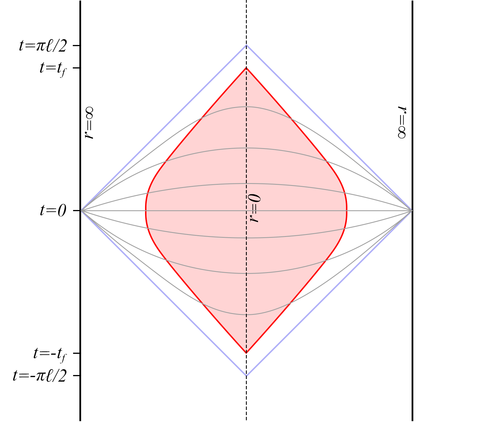
The (null) boundary of the $t=0$ Wheeler-DeWitt patch of a pure AdS spacetime has infinite radius at $t=0$ and shrinks to zero radius at $t=\pm\pi\ell/2$, independently of the dimension $d$. The full (timelike) trajectory of the shell, which starts at $r=R_{*}<\infty$ for $t=0$ and ends at $r=0$ for $t=t_{f}<\pi\ell/2$ is contained within such Wheeler-DeWitt patch.

As a consequence of this result, the entirety of each one of the two (identical) patches $\mathsf{c}_{\mathsf{l}}$ and $\mathsf{c}_{\mathsf{r}}$ of the cosmology is separately covered by the FLRW coordinates describing a hyperbolic slicing of the Wheeler-DeWitt patch (see Fig. 7). The change of coordinates from global AdS to FLRW coordinates is given by $\tan(t/\ell)=\tan(t_c/\ell)/\cosh\rho$, $r=\ell\cos(t_c/\ell)\sinh\rho$, in which case the AdS metric takes the form

where $\text{d}\mathbf{H}_{d}^{2}=\text{d}\rho^{2}+\sinh^{2}\rho\,\text{d}\Omega_{d-1}^{2}$ is the hyperbolic metric of a FLRW time slice.

In the case of empty AdS, this metric describes an open universe and is a solution of the Friedmann equation with negative spatial curvature and a negative cosmological constant, with no additional matter. Since this metric describes a Wheeler-DeWitt patch of pure AdS, it is clearly non-singular. The “big bang” and “big crunch” at $t_{c}=\pm\pi\ell/2$ are simply coordinate singularities corresponding to the tips of the Wheeler-DeWitt patch.

On the other hand, in the case of $\mathsf{c}$, each FLRW time slice $t=t_{c}$ in each one of the two patches $\mathsf{c}_{\mathsf{l}}$ and $\mathsf{c}_{\mathsf{r}}$ is cut off at the location of the shell, implicitly given by $\rho_{\text{max}}(t_{c})=\sinh^{-1}\left[R(t_{c})/\left(\ell\cos(t_c/\ell)\right)\right]$, where $R(t_{c})\equiv R(t(t_{c}))$, and glued to another identical cutoff FLRW slice. Therefore, the cosmology $\mathsf{c}=\mathsf{c}_{\mathsf{l}}\cup\mathcal{W}^{L}\cup\mathsf{c}_{\mathsf{r}}$ is actually closed (i.e. each time slice is compact). Although $\mathsf{c}$ is locally homogeneous and isotropic inside each one of the two patches $\mathsf{c}_{\mathsf{l}}$ and $\mathsf{c}_{\mathsf{r}}$, the presence of the shell introduces an inhomogeneity. In particular, there are two contributions to the expansion and contraction of the universe:¹⁶¹⁶ 16 Here we are considering the full Lorentzian geometry $\mathsf{c}$ obtained by evolving backwards and forward the initial state prepared by the Euclidean path integral at global time $t_{+}=t_{-}\equiv t=0$. If we want to restrict to the contracting phase, it is sufficient to restrict our analysis to $t>0$, corresponding to $t_{c}>0$. the first one is homogeneous and driven by the evolution of the scale factor $a(t_{c})=\ell\cos(t_c/\ell)$, and the second one is inhomogeneous and determined by the contraction of the shell. Unlike the hyperbolic slicing of pure AdS, our cosmology is singular, with the big bang and big crunch singularities approximately corresponding to the initial and final loci of the shell’s worldvolume $\mathcal{W}^{L}$ at $r=0$ and $t=\mp t_{f}$, respectively. Note that these are not the usual homogeneous singularities arising in FLRW universes, but rather inhomogeneous singularities associated with the collapse of the shell, similar to what happens in the geometry enclosed by a collapsing shell during black hole formation. By inverting the coordinate transformation between global and FLRW coordinates:

we obtain that the big bang and big crunch singularities sit at FLRW coordinates $\rho=0$ and $t_{c}=\mp t_{f}$ in each one of the two cosmological patches $\mathsf{c}_{\mathsf{l}}$ and $\mathsf{c}_{\mathsf{r}}$.

Given the construction of the Euclidean section $X$ supported by the heavy shell, which prepares the state $\ket{\psi_0}$ of the quantum fields on the EFT Hilbert space $\mathcal{H}_{\Sigma}$ defined on the initial slice $\Sigma=\Sigma_{\mathsf{l}}\cup\Sigma_{\mathsf{c}}\cup\Sigma_{\mathsf{r}}$, it is natural to consider more general bulk states, $\ket{\psi}\in\mathcal{H}_{\Sigma}$, prepared by additional light operator insertions $\phi(x)$ at different points $x\in X$, as illustrated in Fig. 9.¹⁷¹⁷ 17 Such a naive notion of EFT of “free gravitons and matter” $\mathcal{H}_{\Sigma}$, at $G=0$, should be a reasonable approximation to the true EFT, when $G\neq 0$. At a first glance, this seems problematic, given that the cosmology $\Sigma_{\mathsf{c}}\subset\Sigma$ is a closed space, and that it carries all of the well-know problems of implementing the gravitational Gauss’ law non-trivially in closed spaces. The way in which this setup avoids this issue is to note that all of the modes of the quantum fields in the state $\ket{\psi_0}$ contain some entanglement with the corresponding modes in the AdS region, given that the preparation of the state is thermal-like. Entanglement allows to dress all of the modes on the cosmology, in a state-dependent way, to the physical asymptotic boundaries of the AdS regions. In Sec. 5 we comment on this issue, which affects all of the discussions of entanglement islands, in a simplified toy model. Each bulk state prepared this way defines a corresponding CFT state $\ket{\Psi}\in\mathcal{H}_{\mathsf{L}}\otimes\mathcal{H}_{\mathsf{R}}$ prepared by inserting an appropriate (and in general non-local) CFT operator in the CFT Euclidean path integral. The associated bulk-to-boundary map will be the object of study in Secs. 4 and 5 of this paper.

In the limit of large mass $m\ell\rightarrow\infty$ for the shell, the bulk Euclidean preparation via $X$ effectively decouples both sides of the cosmology (see Fig. 6) and, as a consequence, the bulk state approximately factorizes, $\ket{\psi}\approx\ket{\Phi_-}_{\mathsf{l}\mathsf{c}_{\mathsf{l}}}\ket{\Phi_+}_{\mathsf{c}_{\mathsf{r}}\mathsf{r}}$. In this regime, the reduced density matrices prepared by the bulk Euclidean path integral become simply

where $H^{\mathsf{l},\mathsf{r}}_{b}$ is the time-independent bulk Hamiltonian, associated with the $U(1)$ Euclidean time translation symmetry of each component of $X$. Each $U(1)$ is weakly broken in this limit by the presence of the thin shell in the near-boundary region. The corresponding Hamiltonians are given by local integral on constant Euclidean time slices illustrated in Fig. 9. Additionally, the light fields $\phi^{\mathsf{l},\mathsf{r}}_{I}(x_{I})$ represent the corresponding operator insertions at the points $x_{I}\in X$, where $\mathcal{T}$ denotes the Euclidean time-ordering in the bulk preparation.¹⁸¹⁸ 18 Note that with this time-ordering prescription the Euclidean time runs clockwise on the right component $X_{+}$, and counter-clockwise in the left component $X_{-}$. The factors $Z_{\mathsf{l},\mathsf{r}}(\beta)=\text{Tr}(\mathcal{T}\{e^{-\beta H^{\mathsf{l},\mathsf{r}}_{b}}\phi^{\mathsf{l},\mathsf{r}}_{I}\})$ serve as normalization factors for the states, and correspond to suitable bulk partition functions on thermal AdS spaces.

The bulk state $\ket{\psi}$ constructed this way contains mostly bipartite entanglement between each of the AdS regions and the corresponding side of the cosmology. The reduced bulk density matrices $\rho_{\mathsf{l}},\rho_{\mathsf{r}}$ and $\rho_{\mathsf{c}}$ will have entanglement entropies given by $S(\rho_{\mathsf{l}}),S(\rho_{\mathsf{r}})$ and $S(\rho_{\mathsf{c}})\approx S(\rho_{\mathsf{c}_{\mathsf{l}}}\otimes\rho_{\mathsf{c}_{\mathsf{r}}})\approx S(\rho_{\mathsf{l}})+S(\rho_{\mathsf{r}})$, respectively. Therefore, the cosmology effectively purifies the bulk entanglement of the quantum fields in the AdS regions.

For most of our analysis, we will be interested in excited states $\ket{\psi}$ in which the entanglement $S(\rho_{\mathsf{l},\mathsf{r}})$ and the difference $|S(\rho_{\mathsf{l}})-S(\rho_{\mathsf{r}})|$ can be taken to be large. This can be achieved with the addition of suitable operator insertions along $X$, since these can create light entangled particles between the cosmology and the AdS regions. The effect of adding such insertions is to change the ADM energy of the state. Microcanonically, a gas of particles in AdS is stable, up to energies of order $E\ell\lesssim G^{-1}\sim N^{2}$, before it collapses into a small black hole. Therefore, by adding light entangled pairs between the cosmology and the AdS regions, it is possible to attain a large value of $S(\rho_{\mathsf{l},\mathsf{r}})$ and $|S(\rho_{\mathsf{l}})-S(\rho_{\mathsf{r}})|$. As long as the number of entangled pairs, and thus the total energy, is parametrically smaller than $O(N^{2})$, the semiclassical wavefunction of the state will remain within the cosmological branch.

References

- [1] G. ’t Hooft, “Dimensional reduction in quantum gravity”, Conf. Proc. C 930308 (1993) 284–296, arXiv:gr-qc/9310026.
- [2] L. Susskind, “The World as a hologram”, J. Math. Phys. 36 (1995) 6377–6396, arXiv:hep-th/9409089.
- [3] J. M. Maldacena, “The Large N limit of superconformal field theories and supergravity”, Adv. Theor. Math. Phys. 2 (1998) 231–252, arXiv:hep-th/9711200.
- [4] S. Ryu and T. Takayanagi, “Aspects of Holographic Entanglement Entropy”, JHEP 08 (2006) 045, arXiv:hep-th/0605073 [hep-th].
- [5] B. Swingle, “Entanglement Renormalization and Holography”, Phys. Rev. D 86 (2012) 065007, arXiv:0905.1317 [cond-mat.str-el].
- [6] M. Van Raamsdonk, “Building up spacetime with quantum entanglement”, Gen. Rel. Grav. 42 (2010) 2323–2329, arXiv:1005.3035 [hep-th].
- [7] A. Lewkowycz and J. Maldacena, “Generalized gravitational entropy”, JHEP 08 (2013) 090, arXiv:1304.4926 [hep-th].
- [8] J. Maldacena and L. Susskind, “Cool horizons for entangled black holes”, Fortsch. Phys. 61 (2013) 781–811, arXiv:1306.0533 [hep-th].
- [9] T. Faulkner, A. Lewkowycz, and J. Maldacena, “Quantum corrections to holographic entanglement entropy”, JHEP 11 (2013) 074, arXiv:1307.2892 [hep-th].
- [10] D. Stanford and L. Susskind, “Complexity and Shock Wave Geometries”, Phys. Rev. D 90 no. 12, (2014) 126007, arXiv:1406.2678 [hep-th].
- [11] A. Almheiri, X. Dong, and D. Harlow, “Bulk Locality and Quantum Error Correction in AdS/CFT”, JHEP 04 (2015) 163, arXiv:1411.7041 [hep-th].
- [12] J. Maldacena, S. H. Shenker, and D. Stanford, “A bound on chaos”, JHEP 08 (2016) 106, arXiv:1503.01409 [hep-th].
- [13] F. Pastawski, B. Yoshida, D. Harlow, and J. Preskill, “Holographic quantum error-correcting codes: Toy models for the bulk/boundary correspondence”, JHEP 06 (2015) 149, arXiv:1503.06237 [hep-th].
- [14] A. R. Brown, D. A. Roberts, L. Susskind, B. Swingle, and Y. Zhao, “Holographic Complexity Equals Bulk Action?”, Phys. Rev. Lett. 116 no. 19, (2016) 191301, arXiv:1509.07876 [hep-th].
- [15] P. Hayden, S. Nezami, X.-L. Qi, N. Thomas, M. Walter, and Z. Yang, “Holographic duality from random tensor networks”, JHEP 11 (2016) 009, arXiv:1601.01694 [hep-th].
- [16] G. Penington, “Entanglement Wedge Reconstruction and the Information Paradox”, JHEP 09 (2020) 002, arXiv:1905.08255 [hep-th].
- [17] A. Almheiri, N. Engelhardt, D. Marolf, and H. Maxfield, “The entropy of bulk quantum fields and the entanglement wedge of an evaporating black hole”, JHEP 12 (2019) 063, arXiv:1905.08762 [hep-th].
- [18] G. Penington, S. H. Shenker, D. Stanford, and Z. Yang, “Replica wormholes and the black hole interior”, JHEP 03 (2022) 205, arXiv:1911.11977 [hep-th].
- [19] A. Almheiri, T. Hartman, J. Maldacena, E. Shaghoulian, and A. Tajdini, “Replica Wormholes and the Entropy of Hawking Radiation”, JHEP 05 (2020) 013, arXiv:1911.12333 [hep-th].
- [20] J. B. Hartle, S. W. Hawking, and T. Hertog, “Accelerated Expansion from Negative ”, arXiv:1205.3807 [hep-th].
- [21] P. J. E. Peebles and B. Ratra, “Cosmology with a Time Variable Cosmological Constant”, Astrophys. J. Lett. 325 (1988) L17.
- [22] B. Ratra and P. J. E. Peebles, “Cosmological Consequences of a Rolling Homogeneous Scalar Field”, Phys. Rev. D 37 (1988) 3406.
- [23] S. Tsujikawa, “Quintessence: A Review”, Class. Quant. Grav. 30 (2013) 214003, arXiv:1304.1961 [gr-qc].
- [24] S. Antonini, P. Simidzija, B. Swingle, and M. Van Raamsdonk, “Accelerating Cosmology from a Holographic Wormhole”, Phys. Rev. Lett. 130 no. 22, (2023) 221601, arXiv:2206.14821 [hep-th].
- [25] S. Antonini, P. Simidzija, B. Swingle, M. Van Raamsdonk, and C. Waddell, “Accelerating cosmology from 0 gravitational effective field theory”, JHEP 05 (2023) 203, arXiv:2212.00050 [hep-th].
- [26] M. Van Raamsdonk and C. Waddell, “Possible hints of decreasing dark energy from supernova data”, arXiv:2305.04946 [astro-ph.CO].
- [27] A. Strominger, “The dS / CFT correspondence”, JHEP 10 (2001) 034, arXiv:hep-th/0106113.
- [28] M. Alishahiha, A. Karch, E. Silverstein, and D. Tong, “The dS/dS correspondence”, AIP Conf. Proc. 743 no. 1, (2004) 393–409, arXiv:hep-th/0407125.
- [29] X. Dong, E. Silverstein, and G. Torroba, “De Sitter Holography and Entanglement Entropy”, JHEP 07 (2018) 050, arXiv:1804.08623 [hep-th].
- [30] V. Gorbenko, E. Silverstein, and G. Torroba, “dS/dS and ”, JHEP 03 (2019) 085, arXiv:1811.07965 [hep-th].
- [31] E. Coleman, E. A. Mazenc, V. Shyam, E. Silverstein, R. M. Soni, G. Torroba, and S. Yang, “De Sitter microstates from T + 2 and the Hawking-Page transition”, JHEP 07 (2022) 140, arXiv:2110.14670 [hep-th].
- [32] L. Susskind, “Black Holes Hint Towards De Sitter-Matrix Theory”, arXiv:2109.01322 [hep-th].
- [33] L. Susskind, “De Sitter Holography: Fluctuations, Anomalous Symmetry, and Wormholes”, Universe 7 no. 12, (2021) 464, arXiv:2106.03964 [hep-th].
- [34] L. Susskind, “Entanglement and Chaos in De Sitter Space Holography: An SYK Example”, JHAP 1 no. 1, (2021) 1–22, arXiv:2109.14104 [hep-th].
- [35] E. Shaghoulian and L. Susskind, “Entanglement in De Sitter space”, JHEP 08 (2022) 198, arXiv:2201.03603 [hep-th].
- [36] P. McFadden and K. Skenderis, “Holography for Cosmology”, Phys. Rev. D 81 (2010) 021301, arXiv:0907.5542 [hep-th].
- [37] N. Afshordi, E. Gould, and K. Skenderis, “Constraining holographic cosmology using Planck data”, Phys. Rev. D 95 no. 12, (2017) 123505, arXiv:1703.05385 [astro-ph.CO].
- [38] H. Nastase, “Solution of the cosmological constant problem within holographic cosmology”, Phys. Lett. B 801 (2020) 135168, arXiv:1812.07597 [hep-th].
- [39] H. Nastase and K. Skenderis, “Holography for the very early Universe and the classic puzzles of Hot Big Bang cosmology”, Phys. Rev. D 101 no. 2, (2020) 021901, arXiv:1904.05821 [hep-th].
- [40] J. M. Maldacena and L. Maoz, “Wormholes in AdS”, JHEP 02 (2004) 053, arXiv:hep-th/0401024.
- [41] B. McInnes, “Answering a basic objection to bang / crunch holography”, JHEP 10 (2004) 018, arXiv:hep-th/0407189.
- [42] B. McInnes, “Pre-inflationary spacetime in string cosmology”, Nucl. Phys. B 748 (2006) 309–332, arXiv:hep-th/0511227.
- [43] B. Freivogel, V. E. Hubeny, A. Maloney, R. C. Myers, M. Rangamani, and S. Shenker, “Inflation in AdS/CFT”, JHEP 03 (2006) 007, arXiv:hep-th/0510046.
- [44] N. Engelhardt, T. Hertog, and G. T. Horowitz, “Holographic Signatures of Cosmological Singularities”, Phys. Rev. Lett. 113 (2014) 121602, arXiv:1404.2309 [hep-th].
- [45] S. Cooper, M. Rozali, B. Swingle, M. Van Raamsdonk, C. Waddell, and D. Wakeham, “Black hole microstate cosmology”, JHEP 07 (2019) 065, arXiv:1810.10601 [hep-th].
- [46] S. Antonini and B. Swingle, “Cosmology at the end of the world”, Nature Phys. 16 no. 8, (2020) 881–886, arXiv:1907.06667 [hep-th].
- [47] Y. Chen, V. Gorbenko, and J. Maldacena, “Bra-ket wormholes in gravitationally prepared states”, JHEP 02 (2021) 009, arXiv:2007.16091 [hep-th].
- [48] M. Van Raamsdonk, “Comments on wormholes, ensembles, and cosmology”, JHEP 12 (2021) 156, arXiv:2008.02259 [hep-th].
- [49] M. Van Raamsdonk, “Cosmology from confinement?”, JHEP 03 (2022) 039, arXiv:2102.05057 [hep-th].
- [50] S. Antonini, P. Simidzija, B. Swingle, and M. Van Raamsdonk, “Cosmology from the vacuum”, arXiv:2203.11220 [hep-th].
- [51] S. Fallows and S. F. Ross, “Constraints on cosmologies inside black holes”, JHEP 05 (2022) 094, arXiv:2203.02523 [hep-th].
- [52] S. F. Ross, “Cosmologies inside hyperbolic black holes”, JHEP 11 (2022) 168, arXiv:2209.11620 [hep-th].
- [53] A. Sahu, P. Simidzija, and M. Van Raamsdonk, “Bubbles of cosmology in AdS/CFT”, arXiv:2306.13143 [hep-th].
- [54] C. Akers, T. Faulkner, S. Lin, and P. Rath, “The Page curve for reflected entropy”, JHEP 06 (2022) 089, arXiv:2201.11730 [hep-th].
- [55] T. Hartman, Y. Jiang, and E. Shaghoulian, “Islands in cosmology”, JHEP 11 (2020) 111, arXiv:2008.01022 [hep-th].
- [56] V. Balasubramanian, A. Kar, and T. Ugajin, “Islands in de Sitter space”, JHEP 02 (2021) 072, arXiv:2008.05275 [hep-th].
- [57] V. Balasubramanian, A. Kar, and T. Ugajin, “Entanglement between two disjoint universes”, JHEP 02 (2021) 136, arXiv:2008.05274 [hep-th].
- [58] V. Balasubramanian, A. Kar, and T. Ugajin, “Entanglement between two gravitating universes”, Class. Quant. Grav. 39 no. 17, (2022) 174001, arXiv:2104.13383 [hep-th].
- [59] R. Bousso and E. Wildenhain, “Islands in closed and open universes”, Phys. Rev. D 105 no. 8, (2022) 086012, arXiv:2202.05278 [hep-th].
- [60] K. Papadodimas and S. Raju, “An Infalling Observer in AdS/CFT”, JHEP 10 (2013) 212, arXiv:1211.6767 [hep-th].
- [61] A. R. Brown, H. Gharibyan, G. Penington, and L. Susskind, “The Python’s Lunch: geometric obstructions to decoding Hawking radiation”, JHEP 08 (2020) 121, arXiv:1912.00228 [hep-th].
- [62] N. Engelhardt, G. Penington, and A. Shahbazi-Moghaddam, “A world without pythons would be so simple”, Class. Quant. Grav. 38 no. 23, (2021) 234001, arXiv:2102.07774 [hep-th].
- [63] N. Engelhardt, G. Penington, and A. Shahbazi-Moghaddam, “Finding pythons in unexpected places”, Class. Quant. Grav. 39 no. 9, (2022) 094002, arXiv:2105.09316 [hep-th].
- [64] C. Akers, N. Engelhardt, D. Harlow, G. Penington, and S. Vardhan, “The black hole interior from non-isometric codes and complexity”, arXiv:2207.06536 [hep-th].
- [65] C. Cao, W. Chemissany, A. Jahn, and Z. Zimborás, “Approximate observables from non-isometric maps: de Sitter tensor networks with overlapping qubits”, arXiv:2304.02673 [hep-th].
- [66] V. Balasubramanian, A. Lawrence, J. M. Magan, and M. Sasieta, “Microscopic origin of the entropy of black holes in general relativity”, arXiv:2212.02447 [hep-th].
- [67] M. Sasieta, “Wormholes from heavy operator statistics in AdS/CFT”, JHEP 03 (2023) 158, arXiv:2211.11794 [hep-th].
- [68] J. A. Wheeler, “Geometrodynamics and the issue of final state”, in Les Houches Summer Shcool of Theoretical Physics: Relativity, Groups and Topology, pp. 317–522. 1964.
- [69] Z. Fu and D. Marolf, “Bag-of-gold spacetimes, Euclidean wormholes, and inflation from domain walls in AdS/CFT”, JHEP 11 (2019) 040, arXiv:1909.02505 [hep-th].
- [70] A. Hamilton, D. N. Kabat, G. Lifschytz, and D. A. Lowe, “Local bulk operators in AdS/CFT: A Boundary view of horizons and locality”, Phys. Rev. D 73 (2006) 086003, arXiv:hep-th/0506118.
- [71] A. Hamilton, D. N. Kabat, G. Lifschytz, and D. A. Lowe, “Holographic representation of local bulk operators”, Phys. Rev. D 74 (2006) 066009, arXiv:hep-th/0606141.
- [72] A. Goel, H. T. Lam, G. J. Turiaci, and H. Verlinde, “Expanding the Black Hole Interior: Partially Entangled Thermal States in SYK”, JHEP 02 (2019) 156, arXiv:1807.03916 [hep-th].
- [73] H. W. Lin, J. Maldacena, L. Rozenberg, and J. Shan, “Holography for people with no time”, arXiv:2207.00407 [hep-th].
- [74] H. W. Lin, J. Maldacena, L. Rozenberg, and J. Shan, “Looking at supersymmetric black holes for a very long time”, SciPost Phys. 14 (2023) 128, arXiv:2207.00408 [hep-th].
- [75] J. Chandra, “Euclidean wormholes for individual 2d CFTs”, arXiv:2305.07183 [hep-th].
- [76] I. Kourkoulou and J. Maldacena, “Pure states in the SYK model and nearly- gravity”, arXiv:1707.02325 [hep-th].
- [77] J. Chandra and T. Hartman, “Coarse graining pure states in AdS/CFT”, arXiv:2206.03414 [hep-th].
- [78] V. Balasubramanian, A. Lawrence, J. M. Magan, and M. Sasieta, “Microscopic origin of the entropy of astrophysical black holes”, arXiv:2212.08623 [hep-th].
- [79] T. Anous, T. Hartman, A. Rovai, and J. Sonner, “Black Hole Collapse in the 1/c Expansion”, JHEP 07 (2016) 123, arXiv:1603.04856 [hep-th].
- [80] S. de Haro, S. N. Solodukhin, and K. Skenderis, “Holographic reconstruction of space-time and renormalization in the AdS / CFT correspondence”, Commun. Math. Phys. 217 (2001) 595–622, arXiv:hep-th/0002230.
- [81] K. Skenderis, “Lecture notes on holographic renormalization”, Class. Quant. Grav. 19 (2002) 5849–5876, arXiv:hep-th/0209067.
- [82] G. Darmois, Les équations de la gravitation einsteinienne. No. 25 in Mémorial des sciences mathématiques. Gauthier-Villars, 1927. http://www.numdam.org/item/MSM_1927__25__1_0/.
- [83] W. Israel, “Singular hypersurfaces and thin shells in general relativity”, Il Nuovo Cimento B (1965-1970) 44 no. 1, (1966) 1–14.
- [84] M. Sasieta, “Ergodic equilibration of Rényi entropies and replica wormholes”, JHEP 08 (2021) 014, arXiv:2103.09880 [hep-th].
- [85] T. Takayanagi, “Holographic Dual of BCFT”, Phys. Rev. Lett. 107 (2011) 101602, arXiv:1105.5165 [hep-th].
- [86] M. Fujita, T. Takayanagi, and E. Tonni, “Aspects of AdS/BCFT”, JHEP 11 (2011) 043, arXiv:1108.5152 [hep-th].
- [87] A. Climent, R. Emparan, J. Magán, M. Sasieta, and A. Vilar-López, “to appear”,.
- [88] D. N. Page, “Average entropy of a subsystem”, Phys. Rev. Lett. 71 (1993) 1291–1294, arXiv:gr-qc/9305007.
- [89] S. W. Hawking and D. N. Page, “Thermodynamics of black holes in anti-de Sitter space”, Communications in Mathematical Physics 87 no. 4, (1982) 577 – 588.
- [90] E. Witten, “A Note On Complex Spacetime Metrics”, arXiv:2111.06514 [hep-th].
- [91] M. Kontsevich and G. Segal, “Wick Rotation and the Positivity of Energy in Quantum Field Theory”, Quart. J. Math. Oxford Ser. 72 no. 1-2, (2021) 673–699, arXiv:2105.10161 [hep-th].
- [92] R. Bousso and A. Shahbazi-Moghaddam, “Island Finder and Entropy Bound”, Phys. Rev. D 103 no. 10, (2021) 106005, arXiv:2101.11648 [hep-th].
- [93] H. Geng, A. Karch, C. Perez-Pardavila, S. Raju, L. Randall, M. Riojas, and S. Shashi, “Inconsistency of islands in theories with long-range gravity”, JHEP 01 (2022) 182, arXiv:2107.03390 [hep-th].
- [94] H. Geng and A. Karch, “Massive islands”, JHEP 09 (2020) 121, arXiv:2006.02438 [hep-th].
- [95] J. Chandra and T. Hartman, “Toward random tensor networks and holographic codes in CFT”, JHEP 05 (2023) 109, arXiv:2302.02446 [hep-th].
- [96] H. Liu and S. Vardhan, “Entanglement entropies of equilibrated pure states in quantum many-body systems and gravity”, PRX Quantum 2 (2021) 010344, arXiv:2008.01089 [hep-th].
- [97] A. Kar, “Non-isometric quantum error correction in gravity”, JHEP 02 (2023) 195, arXiv:2210.13476 [hep-th].
- [98] J. Cotler, P. Hayden, G. Penington, G. Salton, B. Swingle, and M. Walter, “Entanglement Wedge Reconstruction via Universal Recovery Channels”, Phys. Rev. X 9 no. 3, (2019) 031011, arXiv:1704.05839 [hep-th].
- [99] C.-F. Chen, G. Penington, and G. Salton, “Entanglement Wedge Reconstruction using the Petz Map”, JHEP 01 (2020) 168, arXiv:1902.02844 [hep-th].
- [100] C. Akers and G. Penington, “Quantum minimal surfaces from quantum error correction”, SciPost Phys. 12 no. 5, (2022) 157, arXiv:2109.14618 [hep-th].
- [101] L. Susskind, L. Thorlacius, and J. Uglum, “The Stretched horizon and black hole complementarity”, Phys. Rev. D 48 (1993) 3743–3761, arXiv:hep-th/9306069.
- [102] J. McNamara and C. Vafa, “Baby Universes, Holography, and the Swampland”, arXiv:2004.06738 [hep-th].
- [103] R. Emparan, C. V. Johnson, and R. C. Myers, “Surface terms as counterterms in the AdS / CFT correspondence”, Phys. Rev. D 60 (1999) 104001, arXiv:hep-th/9903238.
- [104] V. Balasubramanian and P. Kraus, “A Stress tensor for Anti-de Sitter gravity”, Commun. Math. Phys. 208 (1999) 413–428, arXiv:hep-th/9902121.
- [105] S. W. Hawking, “Zeta function regularization of path integrals in curved spacetime”, Communications in Mathematical Physics 55 no. 2, (1977) 133 – 148.
- [106] J. M. Deutsch, “Quantum statistical mechanics in a closed system”, Phys. Rev. A 43 (Feb, 1991) 2046–2049. https://link.aps.org/doi/10.1103/PhysRevA.43.2046.
- [107] M. Srednicki, “Chaos and quantum thermalization”, Phys. Rev. E 50 (Aug, 1994) 888–901. https://link.aps.org/doi/10.1103/PhysRevE.50.888.