./main_img./si_img
Biological Modelling with Nonlocal Advection Diffusion Equations
Abstract
The employment of nonlocal PDE models to describe biological aggregation and other phenomena has gained considerable traction in recent years. For cell populations, these methods grant a means of accommodating essential elements such as cell adhesion, critical to the development and structure of tissues. For animals, they can be used to describe how the nearby presence of conspecifics and/or heterospecifics influence movement behaviour. In this review, we will focus on classes of biological movement models in which the advective (or directed) component to motion is governed by an integral term that accounts for how the surrounding distribution(s) of the population(s) impact on a member’s movement. We recount the fundamental motivation for these models: the intrinsic capacity of cell populations to self-organise and spatially sort within tissues; the wide-ranging tendency of animals towards spatial structuring, from the formations of herds and swarms to territorial segregation. We examine the derivation of these models from an individual level, illustrating in the process methods that allow models to be connected to data. We explore a growing analytical literature, including methods of stability and bifurcation analysis, and existence results. We conclude with a short section that lays out some future challenges and connections to the modelling of sociological phenomena including opinion dynamics.
Keywords: Nonlocal PDEs; Interacting Particles; Aggregation, Flocking and Swarming; Sorting; Territory formation
1 Introduction
A flamboyance of flamingos, a shiver of sharks, a confusion of wildebeest; hundreds of collective nouns have been assigned to define the groups formed by different species. The need for these collective nouns reflects the frequency with which animal groups form across the natural world, from the gathering of a small number of individuals to billions-strong swarms of locusts [181] or a herring shoal that stretches across kilometres [131]. An ability to aggregate is a phenomenon that extends down to the microscopic level, where various bacteria [29, 30] and microorganisms[25] have been observed to organise into aggregates under certain conditions. In the context of our own cells, their capacity to bind and organise is key for the development of many tissues and organs, or their repair following injury.
An essential element in the formation of many groups is the triggering of a movement-based response in an individual, according to signals and behaviours of other members. Directly, a cell may touch another cell and pass information through specialised molecules at the cell surface, or a bird may alter its flight path according to the trajectory of a neighbour. Indirectly, cells may alter motility according to a molecular signal deposited by another cell and animals may respond to territorial scent markings of conspecifics. The cumulative effect of these individual-level behaviours can result in self-organisation at the population scale, for example the rounding up of an initially dispersed population into an aggregate or the adoption of some swarm configuration.
Scientific interest in self-organising phenomena has a long history, and the field forms a pillar of mathematical biology [149]. Naturally, much of the modelling within this field is indebted to the remarkable work[203] of Alan Turing through his reaction-diffusion model, proposed to explain how morphogenesis could occur. Turing’s model involved only molecular components, and showed how an interplay between reaction and diffusion could break the symmetry of a spatially uniform distribution by amplifying natural stochastic fluctuations into an ordered and patterned state. This not only offered a plausible chemical blueprint for how a tissue could become patterned, but also a mathematical blueprint for determining whether self-organisation can occur in some system. Inspired by the aggregation mounds formed from starving Dictyostelium discoideum cells – the initiating step during a multicellular transformation that serves as a paradigm of self-organisation at the microscopic scale [25] – the celebrated chemotaxis model of Keller and Segel [116] followed Turing’s template to illustrate how a system that includes an actively migrating population could also undergo self-organisation. It shows that the positive feedback loop of chemotaxis to a self-secreted attractant could lead to mound formation.
Continuous biological movement models are often formulated as an advection-diffusion equation [149], i.e.
| (1.1) |
where represents the density of some population at position and time . measures the diffusive (undirected) component to movement, while is an -dimensional vector that measures the advective (directed) component to movement. Generally, diffusion may be an diffusion tensor matrix, e.g. describing some anisotropic spread due to the environment [100], however here we will generally take an isotropic diffusion represented by a scalar coefficient , so that where is the identity matrix. The region defines the space in which the population moves: this could range from a line if movement is effectively constrained to a one-dimensional geometry (, e.g. cell movement along nano-engineered channels), a two-dimensional surface (, e.g. animal movement across a landscape) to a three dimensional volume (). If is a bounded domain, then the above model (1.1) will be equipped with appropriate boundary conditions.
For the chemotaxis model of Keller and Segel [116] interactions between individuals are indirect: the individual senses (and moves in response to) another individual through following the local gradient of an attractant secreted by the population. As such, the advective velocity is taken to be proportional to the chemoattractant gradient, i.e. , where is the attractant.
In other instances of group formation, however, interactions are direct: molecular binding between receptors on adjacent cell surfaces can lead to cells pulling themselves together (adhesion or attraction) or moving away from each other (repulsion); animals may also be drawn to each other or move away following a visual sighting of conspecifics. In all such instances, the interaction range becomes a crucial point for consideration: in the case of cells, this could be the range over which a cell can contact a neighbouring cell through touch, or, for animals, the range over which the perception of conspecifics influences its movement behaviour.
Given the existence of an interaction range, an individual has the potential to sense multiple neighbours simultaneously. It is natural, therefore, to suppose that the movement will be based on some integrated response, i.e. according to the distribution of a population (or populations) across its interaction range. Such considerations have led to the increasing adoption of nonlocal PDE formulations [50]. The focus of attention in the present review will be on models in which the nonlocality appears within the advective term, which is calculated according to an integral that measures the influence of the surrounding population on movement. Specifically, we consider the following pair of non-local models,
| (1.2a) | |||||
| (1.2b) | |||||
Motivation for these two model forms can be found through a purely phenomenological argument or by applying a more physical-based reasoning.
Consider first the formulation (1.2a) and its phenomenological motivation (see top row of Figure 1). Here, the nonlocal advection term is founded on the principal that the population at position influences the movements of those at . The induced direction of movement and its magnitude depends on the product of a (vector-valued) function and a (scalar-valued) function . Specifically, specifies a dependence on the distance of to and it identifies the direction of interaction. The function defines the dependence on the population size at . The integral kernel is parametrised according to a sampling radius , representing the interaction range. Net movement results from integrating over all possible positions, and this directly informs the advective velocity at . The parameters and describe diffusion and advection coefficients, respectively.

The phenomenological motivation for (1.2b) follows a similar reasoning (see bottom row of Figure 1), although the function is now scalar-valued, as is the integrated quantity . This formulation can be interpreted analogously to the taxis-like model, with the population moving according to the gradient of a nonlocal measure of the population; for example, this could be a nonlocally-averaged density distribution. Again, the parameters and represent diffusion and advection coefficients, respectively.
A physical reasoning for (1.2a) and (1.2b) follows the consideration of forces and energies; this interpretation takes on particular resonance in the context of cell migration, where translocation of a cell’s body stems from forces exerted as it attaches to other cells and the substrate. Model (1.2a) can be derived through a balance between adhesive and repulsive forces that act at the cell surface (e.g. see [37]): interactions between cells centred at and generate local forces, with the net force according to the integral . This quantity hence describes a force density, with units of , and the coefficient has units of . The corresponding term for (1.2b) is , and will carry the units of an energy density (). Viewed in this light, the advection according to defines a movement according to an energy gradient. The summary review of [41] describes the derivations of models (1.2b) according to energy principle. If the underlying principal is a process of energy minimisation (i.e. down the energy gradient) then parameter and, conventionally, the form (1.2b) is written with the sign of the advection term reversed, i.e.
| (1.3) |
where indicates energy minimisation. Note that we will adopt this convention particular in Section 5.2-5.3, where energy-based analytical methods are utilised. Since energy differences lead to forces, a natural connection between these model forms is laid bare. A note of caution, though, must be applied when applying physical reasoning to biological particles such as animals or cells: attraction between conspecifics or avoidance of predators are measurable behaviours, but they cannot be directly related to a physical force or energy; similarly, a cell is a highly complex structure and its behaviour is not necessarily determined by the need to minimise energy.
Models of form (1.2) have been used since the 1970s to describe ecological systems (see [115, 139, 93, 142, 182, 124, 151, 197]), since the 1990s to describe cellular systems (see [182, 8, 80, 148, 43]), and more recently to describe opinion dynamics (see [77, 88]). A particular point of mathematical interest lies in their capacity for self-organisation, in which modelling a process of self-to-self attraction between members can allow a dispersed population to organise itself into one or more aggregated groups. For this reason, they are commonly referred to as aggregation equations. However, it is important to note that the formulations (1.2) are less restrictive and can be used to model other forms of interaction, such as repulsive interactions that could lead to an enhanced dispersal.
Moreover, the form of these models can be extended to describe heterogeneous populations where the interactions between different populations can be distinct (e.g. see [8, 148, 157, 173]) or incorporated within more complicated models and applied to explain specific phenomena, such as cancer invasion for cellular systems (e.g. see [80, 156, 63]) or dynamics of locust swarms in ecological systems (see [198, 78]). A multi-species generalisation of each of the models (1.2a-1.2b) can easily be formed by extending to , where denotes the density distribution of the out of populations, and considering the systems
| (1.4a) | ||||
| (1.4b) | ||||
In model (1.4a) directed movement is now the combined result of movement-inducing interactions, where is the nonlocal advection coefficient that defines the movement induced on members of population due to interactions with population : and are analogous to the functions described above, and parameters , , and define the interaction range, diffusion coefficient and advection coefficients, respectively. Note that the ’s may be positive or negative, to model inter-species [173] or inter-cellular [157] attraction or repulsion, respectively. Analogous reasoning can be applied to the form (1.4b).
In this article we review the increased employment of nonlocal systems of the above form within biological modelling11 1 Given the scope of this article, we cannot cover all topics in detail and many relevant studies are ommitted.. In Sections 2 and 3 we outline our motivating biological systems, namely cellular adhesion and other cell-based interactions (Section 2) and ecological interactions between animals (Section 3). We describe the key biology and previous modelling that has motivated models of the form (1.2a) and (1.2b) or their multiple species extensions. In Section 4 we explore the derivations of these models from a microscopic perspective, in particular focussing on cellular adhesion. In Section 5 we consider some of the analysis used to understand these models, including linear stability analysis, bifurcation analysis and global existence. We conclude with some key challenges and future perspectives for the field.
2 Nonlocal models for cellular systems
2.1 Adhesion and other cell interactions
Cell adhesion is the fundamental mechanism by which a cell attaches to and interacts with its surroundings[3]. Adhesions form through specialised cell surface receptors; their binding across adjacent membranes not only attaches cells together, but also triggers a range of processes from proliferation to migration. Of the various families of adhesion molecules, cadherins play a particularly prominent role within cell-cell adhesion processes (e.g. see [192]): E-cadherins, for example, form tight adhesive junctions between epithelial cell types; N-cadherins are more commonly associated with transient adhesive interactions between motile mesenchymal cells.
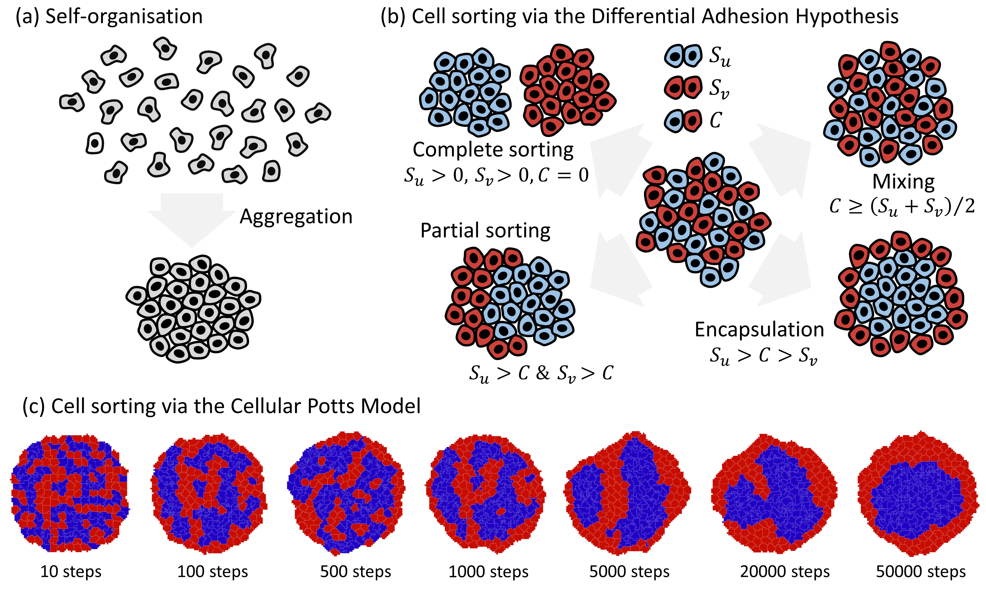
Adhesion is critical for the organisation and maintenance of tissue structure. Naturally, cell-cell adhesion can lead to an accretion process, whereby contact between cells leads to attachment and the formation of a clustered population, Figure 2(a). Moreover, classic experiments indicate a role for adhesion in regulating the spatial organisation of different populations within a tissue [199]. In the differential adhesion hypothesis (DAH)[185, 201] cell sorting is suggested to result from distinct cell surface tensions, deriving in turn from the strength of adhesive interactions. The precise relationship leads to different configurations, see Figure 2(b), and experiments[76] for cell lines that express different levels of cadherins are consistent with this theory. More recently, measurements of the forces within adhesive aggregates [5, 201] have resulted in revision of the DAH to the differential interfacial tension hypothesis (DITH [28]): cell cortical contraction machinery and cell-cell adhesion combine to regulate interfacial tension, and sorting results from rearrangements that lead to a tissue-level minimisation of interfacial tension. Nevertheless, adhesion remains the driving force within the sorting and arrangement of tissues.
Cell-to-cell contacts, though, can also trigger repulsion. For example, contact inhibition of locomotion (CIL)[1] forms a contact-mediated response which not only leads to cessation of cell motion, but also repolarisation and reversal of the direction of motion [40]. Cell-to-cell contacts can also lead to asymmetric responses, where the two cells display contrasting responses. One such example arises in the pigmentation of zebrafish, where interacting xanthophores and melanophores engage in a chase and run[107, 218] interaction, contact between them resulting in the melanophore moving away from the pursuing xanthophore. Other instances of contact-mediated responses that can range from attraction to repulsion include those triggered through Eph/Ephrin interactions [35] or the chase and run dynamics observed in cultures of neural crest and placode cells [195]. A complex set of migration responses that follow direct contacts have been observed among cells of the immune system, impacting on a range of processes that include inflammation and tumour progression [141].
Biological cells are small with an average diameters the order of around ten microns and contact-based interactions occur at a similarly local level. However, contacts can also be formed at considerably greater distances than the mean cell diameter. First, the cell bodies can be highly deformable, where frequent protrusions of the membrane – pseudopodia [51] – locally extend parts of the membrane far beyond the average diameter. Second, a diversity of more specialised membrane protrusions have been identified [219, 121, 180] – variously termed cytonemes, tunnelling nanotubes, microtubes – that in some cases extend the order of 100s of microns. Thus, a contact can be achieved between cells separated by multiple cell diameters, and a non-local description is warranted.
2.2 Models for adhesion and tissue dynamics
2.2.1 Individual level models for adhesion and sorting
Agent-based modelling (ABM) forms a natural approach for adhesive cell populations[184, 188]. The first broadly successful in silico replications of cell sorting can be attributed to Graner and Glazier [91, 86], where a Potts model22 2 A model of statistical mechanics, originally used to understand spin configurations in ferromagnets. was extended to model adhesion. Subsequently dubbed the Cellular Potts Model (CPM), each biological cell occupies multiple grid cells spread across a lattice, therefore giving each cell a shape, volume, and boundary. Evolution of the shape is probabilistically determined via a hypothesised energy functional; the aim is to minimise an energy determined by adhesive contacts along shared surfaces. Selecting relationships in line with the DAH leads to the predicted cell sorting pattern [91, 86]; see Figure 2(c) for a CPM simulation in which adhesion relationships conspire to sort two populations into an encapsulated configuration.
Other ABMs have also shown to be capable of describing adhesion and sorting dynamics[205], sitting at various levels of detail: cells modelled as deformable ellipsoids [161, 160] with centres and semi-axes evolving according to the forces generated by adhesive interactions with other cells and the substrate; on-lattice methods, (e.g. cellular automata type, see [60]); off-lattice centre-based models, where equations of motion describe the position and velocity of a cell’s centre and the cell forms a hard or soft sphere that interacts with nearby cells (e.g. [103, 130, 48]); vertex-based models [73] which feature cell boundaries described by a polyhedron with dynamic vertices. Many of these ABMs form the basis of computational platforms for simulating cellular and tissue dynamics -- CellSys33 3 https://www.hoehme.com/software/tisim [103], CompuCell3D 44 4 https://compucell3d.org/ [191], Chaste 55 5 https://www.cs.ox.ac.uk/chaste/ [140], Physicell66 6 http://physicell.org/, [82] – and their capacity to predict adhesion and sorting phenomena is regarded as a point of calibration between these diverse methodologies [152].
2.3 Continuous models for adhesion and sorting
2.3.1 Local formulations
The representation of a cell population via a continuous density distribution eliminates the issue of scale inherent to agent-based models, where simulating very large cell numbers remains a computational challenge. Moreover, a well posed differential equation system gives access to a wealth of analytical methods (stability and bifurcation analysis, asymptotic approaches, travelling wave analyses) that can yield deeper understanding into the dynamics.
One simple approach to include adhesion has been based on a classic advection-diffusion equation of the form (1.1), where the diffusion and/or advection coefficients depend on the local population density, i.e. the pointwise density. Such models have been proposed on phenomenological grounds (e.g. see [104]), or following a derivation from an underlying random walk description of movement (e.g. see [6, 110]) – see Section 4.1. These models capture certain features of adhesive populations – for example, restricted motility in regions of high adhesiveness – and are both analytically straightforward and simple to incorporate into models. Nevertheless, they have not been shown to allow more complicated sorting behaviour. Moreover, as discussed in greater detail below, the derived diffusion coefficients can sometimes become negative and result in a loss of regularity (for example, [6, 110]). The effects of cell-cell adhesion have also been incorporated in a phenomenological manner into various models for tumour growth (for example [38, 39, 57, 216, 56]), via the incorporation of a surface tension force at the tumour-tissue surface.
2.3.2 Nonlocal formulations
Successful ABM approaches for cell sorting are inherently nonlocal: a cell spread across multiple lattice sites in a CPM, or centre-based approaches where the attractive and repulsive interactions form over an interaction range. This nonlocality can be incorporated into a continuum description using a nonlocal (or integral) PDE formulation. In the context of cell adhesion, the first77 7 As far as we are aware models to adopt this approach were formulated to describe the aggregation of a single homogeneous population in [182] and for multiple cell populations in[8] to explore sorting via differential adhesion; closely related nonlocal models, though, have a biomodelling history that dates back at least as far as the 1970s (for example, see [115, 139, 150, 93]).
The simplest motivation for these models is founded on phenomenological reasoning. Suppose denotes the cellular density at position in space and in time. Ignoring (for simplicity) cellular growth or death and employing standard mass conservation arguments (e.g. see [149]) leads to the balance equation
where denotes the population flux arising from movement. The flux can be decomposed into different terms – for example, a diffusive element to describe undirected movement and an advective component for directed movement – and we arrive at (1.1). Regarding the advective component, suppose that a cell at interacts with another cell at , and that this interaction generates movement; this could be the result of forming adhesive bonds that draw the two cells together. The net movement response follows from summing over all possible interactions and we then postulate an interactive flux proportional to this sum, i.e.
where and are as described following (1.2). Adding to the above a standard (Fickian) diffusive flux, , leads to (1.2a).
A basic model to describe a homogeneous adhesive population sets ,
| (2.1) |
where denotes the unit vector in direction of , and is the indicator function. This stipulates (i) that only those cells within an interaction range impact on movement, i.e. those within contact range for adhesive binding; and (ii) that the strength of interaction increases linearly with the density of cells at , since a higher cell density implies a greater likelihood of forming adhesive bonds. Consequently, we obtain
| (2.2) |
where is the -dimensional ball of radius . The coefficient is a measure of the adhesive strength; switching to turns the interaction into a repelling one, e.g. see [157] in the context of CIL. We note that often the function is normalised, e.g. according to the volume of the interaction space and we therefore place a dependency on in the parameter for generality. Other natural choices would be to assume that the strength of interaction decreases with increasing separation, due to reduced likelihood of forming a contact: for example, the magnitude of decreasing exponentially with the distance . Nonlinear choices for are also logical, e.g. forms to reflect an upper bound in the adhesive pull that can be generated, see below.
2.3.3 Capacity for self-organisation and sorting

A key strength in the model (2.2) lies in its capacity for self-organisation (see Section 5.1 for more details): for , a dispersed population remains dispersed, see Figure 3(a) while for it becomes concentrated into a tight aggregate, see Figure 3(b). Under the basic model (2.2), the aggregates evolve into a highly concentrated aggregate88 8 For a discussion of global existence, see Section 5.2, even for . This can be attributed to the lack of any mechanism that reins in the amount of adhesive pull that can be generated.
Adding further detail to the model assumptions can help prevent over-accumulation within the aggregates. For example, setting to be a saturating function (which can be motivated naturally through adhesive receptor occupancy, see Section 4), then
| (2.3) |
This leads to aggregations that are capped at lower densities, see Figure 3(c). Other possible modifications include the addition of ‘volume-filling’ (e.g. see [157, 43]), or adapting diffusion to a density-dependent and degenerate form (e.g. see [144, 32, 148, 33, 43]). The addition of the latter to (2.3) leads to
| (2.4) |
This adaptation limits a diffusive spread at the cluster boundary, the aggregate taking on a compact form with a sharp interface, Figure 3(d).

As noted earlier, nonlocal formulations can be easily extended to include multiple populations, see (1.4). A natural question, therefore, is whether cell sorting can be replicated under a nonlocal formulation. Consider two populations and and assume equivalently simple forms to (2.1), then a basic model to describe cell sorting can be stated by the equations
| (2.5a) | ||||
| (2.5b) | ||||
In this model , and represent the - self-adhesion strength, the - self-adhesion strength, and the - cross-adhesion strength, respectively. Note that the interaction ranges are the same (and equal to ) and cross interactions are symmetrical, although such assumptions can be relaxed and repelling interactions can also be introduced (for example, see [157, 47]). Unfortunately, this basic formulation (2.5) proves overly simple to capture the nuances of cell sorting. As for the basic homogeneous model (2.2), the linear choices for the nonlocal terms lead to excessive attraction and the populations become highly concentrated, see Figure 4, top row. The model, as such, is unsatisfactory when it comes to resolving the subtly distinct cell sorting patterns shown in Figure 2(b).
Consequently, ‘successful’ nonlocal models [8, 81, 157, 148, 43] that are more broadly capable of replicating the spectrum of arrangements predicted by the DAH include modifications to the various terms in model (2.5). For example, this has included adding biologically-meaningful features such as a limitation or saturation to the adhesive pull (see [8, 81]), introducing volume-filling effects that prevent cell aggregation beyond a critical (packed) level (see [157, 43]), or modifying diffusion terms to include total population pressure effects (see [148, 33, 43]). To provide one concrete example, by adapting the saturating functional forms above and including population-pressure effects to create sharply segregated boundaries (see [148, 43]), we have
| (2.6a) | ||||
| (2.6b) | ||||
This more ‘advanced’ sorting model is capable of replicating the nuances of cellular sorting under different adhesive relationships, e.g. for two populations it can generate the full spectrum of arrangements from mixed to complete sorting see Figure 4.
Summarising, nonlocal models are capable of reaching two touchstones of adhesive behaviour: (i) capturing the adhesive or sticky-like properties of cells in close contact, and (ii) replicating cell-sorting phenomena for heterogeneous adhesive populations as predicted by the DAH.
At this point we return to our earlier implication that local formulations are incapable of adequately describing adhesion and sorting dynamics, stressing that this applies to ‘näive’ local formulations. In fact, various local models can be shown to exhibit sorting. One method (though not directly describing adhesion) is through extension of a chemotaxis framework: effectively, a ‘differential chemotaxis’ system in which two populations have distinct chemotactic responses to multiple chemical factors (e.g. [155, 120]), so the interactions are indirectly mediated. Directly relevant to adhesion, an intriguing (fourth order) local model has been recently formulated in [70] and demonstrates an impressive capacity to simulate the range of cell sorting patterns described here: we return to this in the discussion.
2.4 Further applications to cellular systems
Classic cell sorting experiments [199] were first performed using embryonic cell populations, naturally leading to a conjecture that adhesion and sorting are fundamental during embryonic development (for a historial retrospective, see [186]). Consequently, a principal application for nonlocal models for cell adhesion lies in developmental processes. In fact, the first nonlocal model for adhesion[182] was proposed in the context of self-organisation of scale cells during lepidoptera (moth and butterfly) wing morphogenesis. Nonlocal adhesion models have subsequently been developed, as described above, to show fundamental cell sorting (see [8, 81, 148, 43]), somitogenesis99 9 A fundamental early embryonic stage of segmented animals, whereby mesoderm tissue is sequentially discretised into blocks of cells along the head to tail axis. [9], skeletal morphogenesis1010 10 The embryonic process during which the skeleton is formed. [87, 22], aspects of neural development [132, 200], and vasculogenesis1111 11 Formation of the primitive vasculature network [209]. Notably, some of these applications have been directly formulated alongside experimental data, linking predictions formed from models to targeted experiments. For example, a nonlocal model of adhesion was formulated[87, 22] to describe mesenchymal cell movements which indicated a crucial aggregating role for adhesion during early skeletal morphogenesis . Experimental-theoretical studies that feature nonlocal adhesion models have also been used to understand brain development, in particular the crucial role of N-cadherin mediated adhesion in the positioning of neuronal populations during mammalian cortex development [132] and the visual centre of the fly Drosophila melanogaster [200].
Abnormal regulation of adhesive processes may be a factor for various pathologies, in particular cancers [108]. For example, a point of significant focus has been on the epithelial-mesenchymal transition (EMT), where upregulation of N-cadherin accompanied by downregulation of E-cadherin allows cells to adopt a more migratory form, linked to increased invasiveness and metastasis [127]. Many mathematical models have been developed to address the roles played by cell-cell (and cell-matrix) adhesion during invasion and a growing number (e.g. [80, 118, 156, 63, 23, 24, 102, 190]) have applied nonlocal formulations: to understand how adhesion alters the shape of cancer invasion (e.g. [80, 156]); the role of cell-cell adhesion during glioma growth (e.g. [118, 190]); shaping different forms of tumour infiltration patterns in ductal carcinomas (see [63]); and, two population models, featuring cancer populations at different states of mutation (see [23, 24]). Other points of application for nonlocal models of adhesion and cell interactions include wound healing (e.g. [64, 65, 212, 213]) and modelling the interactions between liver cells [92].
3 Nonlocal models for ecological systems
3.1 Swarms, flocks, and herds
Swarming, herding, and flocking phenomena are perhaps the most obvious examples of collective behaviour in ecological systems [189]. The central idea is that animals, like cells, often exhibit social interactions that cause them to aggregate. At their most basic level, social interactions may simply cause animals to be found in a particular area of space at some point in time, rather than using all the available area [197]. At a more advanced level, these interactions can cause a very wide range of complex patterns to emerge, famously exemplified by starling murmurations, but present throughout the animal kingdom [12, 189].
An enormous number of models have been formulated to understand collective animal movements [208, 17], a substantial proportion of which are based on systems of ‘interacting particles’1212 12 In probability theory, the term ‘interacting particle system’ has a specific definition in the context of continuous time Markov jump processes. When we refer to interacting particles within this article, we will often slip into a slightly broader sense: complex systems composed of agents that interact with each other according to their relative positions and/or velocities.: the position of each agent is governed by a dynamic (usually, stochastic) equation featuring terms that account for how the trajectories of neighbours influence movement (well known models include those in [7, 178, 95, 207, 54, 53, 59, 145]). Typically, the interactions lying at the heart of these models are formulated according to the ‘first principles of swarming’ [45]. At the shortest range, interactions are often repulsive, as animals will want to avoid physical contact. At a slightly longer range, animals will align their movements with one another. Then if animals become too far apart, they have a tendency to move towards one another to maintain the group cohesion (attraction). These three zones of nonlocal interactions1313 13 One of the earliest and most influential model explicitly built along these principles– the ‘Boids’ model of Reynolds [178] – was developed with the main aim of generating realistic flocking-like behaviour for the computer graphics industry, rather than the more elementary aim of understanding movement dynamics; numerous interactive online simulators of this model exist, e.g. https://boids.cubedhuang.com/. A particularly notable branch that evolved from that work was the application of swarming models to optimization, i.e. particle swarm optimization [117]. combine to give both stationary and moving aggregations, as well as a vast swathe of spatio-temporal patterns, mimicking many of those that have been observed in nature (see [189, 208, 17]).
A smaller – but still substantial – literature has approached the same central problem of swarming and animal movement via a continuous framework, using ideas that surround nonlocal advection (see [142, 197, 68, 173, 210]). In fact, the earliest nonlocal biological aggregation models were developed to describe swarming-like behaviour (see [115, 139, 150, 142, 124]) and were based on the nonlocal PDE (1.2a). For example, in [142] even or odd forms of interaction kernels were explored for their capacity to generate drift-type (coherent movement of the swarm) or aggregation-type (cohesion of the swarm) behaviour. A further branch of nonlocal PDE methods are founded on hyperbolic kinetic transport equations (see [68, 67, 19]). In these models, the nonlocal terms do not enter the advection terms, but the turning behaviour of the population; consequently, they benefit from a closer description of individual behaviour and can, for instance, explicitly incorporate the above principles of swarming commonly used in particle models. However, these models represent significant and non-trivial extensions of Equations (1.2-1.4) – although it is possible to connect them [31] – and are more challenging to explore from an analytical and numerical perspective. As such, we do not go into details, instead we refer the reader to a recent book[67] that summarises developments in this area.
3.2 Home ranges and territories via stigmergy and memory
As well as the visually-impressive examples of collective movement, aggregation phenomena can also occur over longer spatial and temporal scales, becoming apparent as one observes animal locations over a period of time. For example, by plotting locations over an increasing time window, it often transpires that animals do not use as much of the available area as their locomotive capabilities allow. Instead they confine themselves to a smaller area called a home range, which they may maintain for a season or even a whole lifetime [34, 26]. This causes the spatial distribution of the animal to tend to a stationary, non-constant distribution, such as can be modelled by Equation (1.2b) or variants thereof [27].
Home ranges can emerge due to a range of biological processes. For example, animals may tend to re-visit locations remembered to be good for foraging [179]. Once they have memory of sufficiently many locations to meet their foraging needs, they may decide to stay in the vicinity of those locations (see [206, 137]). Additionally, they may need to construct a central place near to where they forage, such as a den or nest site, for reproductive purposes. The requirement to return to this central place then provides yet another mechanism of locational aggregation [143]. Finally, animals may leave traces of their past locations in the landscape (e.g. through scent marks) and use these as markers to keep them in their home range: a process called stigmergy [194]. In any of these cases, the decisions of the animal to move will tend to be spatially non-local, due to the animals’ ability to sense their surroundings as they move, through sight, smell, or memory of target locations (see [168, 14, 69]).
To model these biological processes, it is common to couple a nonlocal advection-diffusion equation for the location distribution to an ordinary differential equation (ODE) modelling the process of memory or stigmergy. The recent review of [210] gives a thorough exposition of these process, but perhaps the simplest example is
| (3.1) | ||||
| (3.2) |
where is the probability distribution of the animal and denotes the cognitive map [210], which models either the density of marks left on the terrain or the amount of memory the animal has about location at time . Other notation is as in Equation (1.2b).
Territoriality provides another reason why animals may confine themselves in space over long periods of time. Here, the presence of neighbouring conspecifics forces animals into a confined space (see [2, 171]). There are various mechanisms by which this can happen, but from a modelling perspective they fall into two categories. The first is via stigmergy: indirect interactions mediated by some form of marks on the terrain, such as urine, faeces, or a trail [143, 174]. In this case, animals avoid the marks left by others in the recent past, and usually these marks decay over time. The second is via memory of direct interactions, such as displays or fights [119]. Animals remember the locations of these displays or fights and may tend to avoid them in the near future [172]. In either case, as with home range formation, the movement of animals in response to these interactions is usually spatially non-local.
These territorial mechanisms can be modelled using exactly the multi-population system in Equation (1.4b) with for to model mutual avoidance, and . However, as with home range models, it is often valuable to model the process of memory or stigmergy explicitly via ODEs. A simple example can be given by combining the ideas behind Equations (3.1)-(3.2) with those of Equation (1.4b), as follows
| (3.3) | ||||
| (3.4) |
where denotes the cognitive map of species , and models the marks left by individuals from territorial unit , whilst and are constants. However more complicated versions can be considered that include extra biological realism [172, 174, 210].
3.3 A general framework for non-local interactions in ecology
As well as territory formation, the multi-species case from Equation (1.4) enables a variety of other ecological phenomena to be modelled over timescales where births and deaths are negligible (e.g. for mammals and birds, this may be over a season or year) [173, 83]. For example, the movements of co-existing predators and prey can be modelled by assuming prey advect away from predators and predators towards prey [61]. Likewise, competing species may advect away from one another and mutualistic animals may have a tendency to move towards one another. In forager and scrounger interactions, the latter follow the former to exploit their foraging efforts (e.g. see [193]). In ecosystems consisting of many species, there will be a complex network of such interactions that can cause a wide range of emergent patterns (Figure 5c-e).

As a consequence, Equation (1.4b) has been proposed as a key study system for understanding spatial distributions of interacting groups of animals that may emerge over such timescales [173]. These groups of animals may be territorial groups, populations, or whole species (but we often just use ‘species’ for all such groups for simplicity and consistency with the rest of this review). The overall aim is to be able to provide links between the network of interactions between moving species (Figure 5b) and their pattern formation properties.
For example, Figure 5a shows the predictions of linear stability analysis for four different systems of three populations (model (1.4b) for ) shown schematically in Figure 5b. This gives a simple categorisation into ‘no patterns’ (all eigenvalues having negative real parts) ‘stationary patterns’ (the dominant eigenvalue is real and positive) or ‘fluctuating patterns’ (the dominant eigenvalue is non-real with positive real part). However, further away from linear stability regime, patterns in three-population systems can be quite complex and varied, including stationary patterns of aggregation and segregation (Figure 5c), travelling-wave-like solutions (Figure 5d), perpetual irregular oscillations (Figure 5e), and more [173, 84].
4 Derivations from the individual level and connecting to data
4.1 Random walks
When Karl Pearson coined the term ‘random walk’ in 1905 [163], the central question involved biological movement: if, within a particular time step, each mosquito moves some distance in a randomly chosen angle, can we estimate the distribution of a mosquito infestation? Fundamental work by Patlak [162] extended the question to include biases from the environment and persistence. Across the last few decades a vast number of studies have aimed to connect the random walk movements performed by individuals to population level measures and distributions, for both cell and animal movement (e.g. see [154, 18, 202, 52]). Specifying a position jump random walk (PJRW, see [52, 151, 158, 187, 154]) forms a particularly well trodden path. In the context of the present review, this approach can be used to motivate both local and nonlocal models for aggregation [37]. To illustrate this, we first lay down a general formalism.
Let us consider the probability that a random walker has its centre at position at time . If we have a population of independent walkers, this probability can be equated with the population density , and we maintain this notion. Note that the definition in terms of the centre implicitly assumes that the walker can have some finite extent, i.e. it is not necessarily a point object. For now we shall avoid any discussion of boundary conditions and assume an individual can move anywhere in space: movement is within . The time continuous Master equation for the PJRW has the following form [154, 106, 204]
| (4.1) |
where is a probability density function for a jump from to . Note that can depend on , but we omit this dependency from the notation. is a rate parameter. We remark that individuals can remain at their current location through setting , which we refer to as a zero-length jump. We follow the approach of [37] and rewrite the integral kernel according to the jump heading . Specifically,
where we assume that
can be split into even and odd components,
| (4.2) |
Then
| (4.3) |
with an even part and an odd part , which satisfy
| (4.4) |
We employ this decomposition in the general master equation (4.1) and make two further assumptions. First, that transition rates do not depend on the increment , just the starting location : this describes a myopic random walk. Second, non zero-length jumps are small and of fixed length , and Taylor expansions can therefore be applied. Details of the expansions can be found in [37] where, in the limit as and , we arrive at the advection-diffusion equation
| (4.5) |
We denote by the dimensional unit sphere in . The advection velocity is given by
and the diffusion term by
Particular care must be paid to the limit scalings, as they suggest different powers of : for the limits to simultaneously exist the odd part must be small (i.e. ) with respect to the even part. If the odd part is of order one or larger, the diffusion term vanishes and a pure drift equation (a drift-dominated case) is derived. When the odd part is of order or smaller, the drift term vanishes and a diffusion-dominated case arises. The value of separating with respect to its odd and even parts becomes clear: the even component enters the diffusion term, while the odd component determines the advection term. Generally the odd and even parts can involve nonlocal terms that represent sensing up to a certain radius. We will return to this in the next section but one.
4.1.1 Local models
We illustrate the above scaling through an interesting local case, which leads to taxis-type models. To introduce dependency according to some controlling factor, we take the standard assumption[187] of supposing that the jump probability distribution explicitly depends on a control species, which we denote . For simplicity, we will restrict in this section to a symmetrical case where we set for all non-zero length jumps (i.e. depends only locally on through ). When movement occurs, all headings are chosen with equal probability, but this probability varies with the local level of the control species . There is no odd component to and the limiting equation (4.5) in this case is of the form
| (4.6) |
Therefore – despite an absence of directionality to the jump – a taxis-like process emerges at the macroscopic level: advection according to the gradient of . The control species can be distinctly interpreted according to the movement process. For example, it may simply define a fixed environmental variability, e.g. regions where movement is easier or more difficult. It could also change according to the distribution of the population – for example, a scent deposited by an animal or a chemical released by a cell – and therefore defined by an evolution equation such as (3.2). We refer to [99, 15] for detailed reviews on chemotaxis models.
Using cell adhesion as a case study, a simple but naïve approach would be to directly equate the control species with the population density. Specifically, we consider and hence obtain the density-dependent diffusion equation
| (4.7) |
Considering the ‘stickiness’ property of adhesion, a logical choice for would be a decreasing function that reflects reduced capacity to move as a cell forms adhesive attachments with its neighbours. For example, a choice results in : this reduces diffusivity in regions of higher population density, and corresponds with certain choices[104] in macroscopic (phenomenological) approaches to adhesion.
Derivations of local models for adhesion that rely on the PJRW framework have been considered previously (e.g. see [6, 110, 113]). While more sophisticated than the above – for example, more complicated jump probabilities or accounting for correlations in movement – they essentially lead to the same result of a density-dependent diffusion equation. Clear advantages lie in that they can lead to models that can be fitted against experimental data (e.g. obtained from cell assays [112, 111]), and that the derived PDE form is relatively tractable, both analytically and numerically.
However, while density-dependent diffusion captures one expected consequence of adhesion, it is more questionable in the context of self-organisation or cell sorting phenomena. The possibility of biological aggregation within both the underlying discrete master equation and its corresponding continuous model has been considered in various studies (for example see [126, 159, 105, 6]), and for (4.7) it is straightforward to use linear stability analysis (see Section 5.1) to show that for (4.7) this will depend on the shape of : instability of the uniform steady state, and hence self-organising capacity, requires . This is not possible for , but can be satisfied when for . However, at this point the PDE (4.7) will become illposed and unpractical for application.
4.1.2 Nonlocal models
Intuitively, it is the pointwise nature of the dynamics that proves problematic in the above. The random walker responded only to the strictly local information acquired at its centre: it is a point particle, and the population can potentially become trapped at singular locations of ‘infinite stickiness’.
A cell or organism, though, has a spatial extent and, even if interacting only through direct contact, will interact across some volume of space. This naturally leads to the question of how one can extend derivations from PJRWs in a manner that retains this nonlocality. We will again use cell adhesion as a case study and follow the approach in [37]. As noted earlier, the formation of adhesion bonds between membranes leads to the generation of (local) forces that draw cells together; cellular membranes are highly dynamic, extending and retracting protrusions that span shorter (e.g. lamellipodia) and longer (e.g. filopodia) ranges. Adhesive attachments, therefore, can create forces at a position that act to displace a cell centred at where the distance is potentially several mean cell diameters away. The method in [37] is to consider a biased random walk where the bias results from summing over all possible local forces that can impact on the cell centred at , which enter the odd component of in (4.3). Following the scaling, one obtains a nonlocal advection velocity of the form
| (4.8) |
In the above, denotes an adhesive strength per adhesion bond, denotes the direction and length of the cell extension, denotes the bound adhesion receptors that are generated with cells at location , indicates the amount of free space available for cells to extend into this area, denotes the ability of a cell to express adhesion receptors a distance away from its centre, and accounts for that bonds generated at will lead to a bias corresponding to that direction.
The formulation in (4.8) is rather general, therefore admitting varying degrees of biological detail. For example, assuming compact support for the cell extension, no space limitation (), and using mass action kinetics to set the number of bonds to be proportional to the cell density (), one essentially arrives at a model of the form (2.2). If, rather, one takes the adhesion binding to be governed by a Michaelis-Menten type binding mechanism, , then we arrive at a model similar to that specified in (2.3).
Consequently, through an explicit derivation from a PJRW it is possible to motivate and clarify the implicit assumptions that underlie various nonlocal models for adhesion, in particular those originally developed with phenomenological reasoning and applied to various phenomena (Section 2.4). More generally, given that the integral (4.8) will typically be a nonlinear function of the cell density and the ability to form attachments varies with the distance from the cell centre, one can straightforwardly obtain the general formulation in (1.2a).
4.1.3 Step selection functions: connecting to data on organism movement
The formalism of a PJRW also allows for relatively straightforward parameterisation of advection-diffusion equations based on data, an approach that has been used both for experimental data obtained for cell systems (say, using cellular assays, e.g.[111]) and locational data for animals (e.g. [176, 169]).
Taking the example of animal movement, these data typically arrive as a time series of locations. If this time series is relatively low frequency, e.g. of the order of one location every few minutes or hours, we might use the funtion (Equation 4.1) to model movement between successive measured locations, from to (see [74]). Alternatively, if the time series is very high frequency, e.g. many locations per second, which is increasingly common [214], can be used to model movements between successive places where the animal makes a turn [147]. In this latter case, we are more accurately modelling behavioural decisions of animals, as they will likely turn for a reason [215].
Either way, a huge amount of ecological insight has been gained in recent years by fitting functions that describe a position-jump process to time series of animal location data (e.g. see [75, 196, 72]). Moreover, further understanding can be gained by scaling these processes up to distributions of broad-scale space use patterns via advection-diffusion equations, using similar techniques to those described in Section 4.1 [169]. The specific position-jump model that has gained particular interest from the ecological community goes under the name ‘step selection function’ (SSF) and has the following form1414 14 The nomenclature in the literature is not always consistent here. Sometimes SSF refers to Equation (4.9), sometimes to the numerator of this equation, and sometimes just to the function .
| (4.9) |
where represents something about the organism’s movement capability, often a distribution of ‘step lengths’ 1515 15 More generally, could be a distribution of step lengths and turning angles, so that is dependent upon , , and also the bearing on which the animal travelled to . But to keep the exposition simple, we will assume here that only depends upon and . , and is a ‘weighting function’ which encapsulates anything that covaries with movement. Typically, is written in the following exponential form
| (4.10) |
where is a vector of functions, each of which represents a movement covariate, and is a vector denoting the relative contribution of the effect of each covariate on movement. In many practical examples of step selection, are simply static environmental features measured at the end point of the step (so can be written as ) (see [196, 72]). However, they can also represent features along a step, such as barriers [21], or dynamic quantities such as memory [136] or the presence of other organisms [170]. Memory processes lead to self-interaction, which may give rise to a single species aggregation-type equation (1.2). If co-moving animals or interacting populations are being modelled, it is necessary to write a different step selection function for each entity (individual or population) [175]. These coupled step selection functions then lead to multi-species equations, like Equation (1.4) [176].
A reason for the popularity of the functional form in Equations (4.9-4.10) is that parametrisation can be done simply and quickly using conditional logistic regression. Details of this technique are given elsewhere (see [74, 10]), but in short it involves first approximating the integral in the denominator of Equation (4.9) by sampling from , and then recognising the resulting function as the likelihood of a case-control study where the samples are the controls.
Although there are many empirical studies using step selection functions to infer information about animal movement (e.g. see [196, 72]), there are far fewer that take the next step of deriving the associated advection-diffusion equation to understand broad-scale space use patterns [169]. Perhaps the reason for this is that such studies combine empirically-driven questions with relatively-advanced mathematical analysis, thus require strong interdiscplinary collaborations between applied mathematicians, empirical ecologists, and statisticians. The flip-side is that there is huge, fertile ground for mathematicians to collaborate with those ecologists involved in step selection studies, enhancing their data analysis and answering new scientific questions [170].
4.2 Derivations from interacting particle system models
As mentioned earlier, many of the ABM-based approaches to cellular and animal aggregation phenomena fall into the broad class of systems of ‘interacting particles’. Deriving continuous models from these models forms a very large field, and a growing literature has emerged in which nonlocal models related to (1.2) are obtained. It is significantly beyond the scope of the present article to provide a comprehensive examination of this literature. Rather, we provide a few apposite examples and refer to others (e.g. [45, 146]) for a more general review.
To provide some context, we consider the following concrete example1616 16 We note that this particular example comes from a model formulated for opinion dynamics, rather than biological aggregation. However, the underlying principles are the same: a tendency to converge, whether in position or opinion, when agents are sufficiently close. in one dimension; we refer to [146, 77] for more details. Let the position of agent in a population of size at time be determined by the stochastic differential equation
| (4.11) |
In (4.11), the ’s denote independent Brownian motions and model an uncertainty to the particle position (with strength ). Interactions are incorporated through the summed term, where gives the strength of interaction between agents and ; the factor averages across all possible interactions. This general form can be tailored to describe an attraction process between sufficiently close individuals – e.g. as relevant for cell adhesion – by setting the interaction to be a function of the distance of separation, , with compact support: i.e. no attraction above a critical interaction range.
To obtain a continuous model, one can consider the following empirical probability measure for the positions of all agents at time :
where is the Dirac measure with point mass at position . Through application of mean field asymptotic theory, it can be shown [77] that as the probability measure (weakly) converges to a deterministic density , which under certain conditions is governed by a nonlocal PDE of the form (1.2a).
A number of other derivations from IPS models have also led to equations related to (1.2). In one paper[138] the starting point was an off-lattice centre-based model (see Section 2.2.1), in which the motion of each particle is governed by Newton’s second law of motion under viscous forces, forces from self-propulsion and forces from interactions. The latter allowed adhesion-type interactions to be included, which followed the standard assumption of varying with the degree of separation. A hierarchical system of nonlocal PDEs was obtained to describe the distribution of a population of interacting cells and, again following a mean field approximation, a nonlocal aggregation model of the form (1.2a) is obtained.
Nonlocal aggregation models of the form (1.2b) can also be motivated from an IPS (e.g. see [144, 32]). The motivation in [144] lay in the aggregating tendency of ants (Polyergus rufescens), with each ant’s position evolving according to a stochastic differential equation driven by Brownian motion and an interaction drift; drift dominated over random wandering when other individuals enters an ant’s interaction range. Both aggregating and repelling effects were included, with the former operating when another individual enters an attracting range and a repulsion term for when they become too close. Assuming a large population , then in the limit the following equation was derived for the population density:
where follows from the Brownian motion and the density-dependent (degenerate diffusion) and nonlocal drift terms follow from the repulsion-attraction interaction; derives from the aggregation interaction kernel. The above essentially combines the formulation (1.2b) with an additional degenerate diffusion term, as previously described in Section 2.3.3.
5 Analytical properties
5.1 Linear stability analyses
A linear stability analysis can be used to demonstrate basic criteria for aggregation from a dispersed initial state, i.e. self-organisation properties. We first consider the formulation (1.2a) and, for maximum clarity, utilise the simple assumptions that lead to (2.2) and constrain to a one-dimensional infinite domain; the latter restriction circumvents the complications that arise from specific boundary conditions. Consequently, (2.2) becomes
| (5.1) |
while under equivalent assumptions the formulation (1.2b) becomes
| (5.2) |
Assuming that the population is initially distributed about a uniform steady state , we perform a Turing-type stability analysis (e.g. [149]) by linearising about the uniform steady state and looking for solutions to the linearised equation with mode and eigenvalue as as . This yields the characteristic equations for the eigenvalue-wavenumber relationship
| (5.3) |
for (5.1) and (5.2), respectively. Inhomogeneous perturbations of the steady state grow if there are unstable wavenumbers , i.e. those for which . Straightforward inspection of the above reveals that this will hinge on the competition between stabilising (diffusion) and destabilising (aggregation) processes. In particular, the parameter regions in which self-organisation occurs1717 17 Note that this is under the infinite domain assumption, thereby allowing patterns to grow with unbounded wavelengths. are given by
| (5.4) |
for the formulations (5.1) and (5.2), respectively. While phenomenologically similar, these two conditions are subtly distinct according to the relationships between the strength and range parameters.
Commonly, the nonlocal terms in models of type (1.2) are normalised, e.g. according to a measure of the size of the interaction space: in the context of (5.1-5.2), it is standard to choose and . Under this choice, the instability conditions for the interaction strength ( or ) and interaction range () have some clear distinctions for the two models (5.1-5.2) and become
The condition for (5.2) is independent of , while for (5.1) the capacity for self-organisation is lost as the interaction range decreases. We illustrate the parameter spaces in Figure 6(a).
Characteristic equation curves for particular parameter values illustrate these behaviours: large and sufficient or allows patterning for both models; correspondingly, a finite range of unstable wavenumbers is observed (Figure 6(b,c), black curves). Decreasing , the range of unstable wavenumbers either expands for (5.2) (Figure 6(e)) or shrinks and disappears for (5.2) (Figure 6(d)).

Further insights are obtained through expanding inside (5.1-5.2) and truncating at different orders. The simplest nontrivial case (using , ) leads to the second order local approximations
| (5.5) |
for (5.1) and (5.2), respectively. These immediately recall the density dependent diffusion forms derived in Section 4.1.1. Instability regions for these equations are identical to those defined by (5.4), however this coincides with the region in which the models become illposed (negative diffusion); this manifests through corresponding characteristic equations whereby all wavenumbers are unstable, see red curves in Figure 6 (b-e).
The expansions can also be truncated at higher order terms, and in particular the fourth order approximations become
| (5.6) |
and
| (5.7) |
for (5.1) and (5.2), respectively. Instability regions are again as those defined by (5.4). However, we now note that the destabilising second order term is countered by a stabilising fourth order term. The characteristic equations in this case generate finite ranges for unstable wavenumbers (blue curves, Figure 6 (b-e)), curves closely following those of the nonlocal model (black curves). The distinct limiting behaviours as become clear from (5.6)-(5.7): the fourth order approximation to (5.1) implies convergence to a simple diffusion equation, with constant (and nonnegative) diffusion coefficient ; the fourth order approximation to (5.2), however, converges to a density dependent form (second equation in (5.5)) with potential illposedness. We note that the fourth order approximations to nonlocal models have been studied in detail, e.g. in [182] for one variable models and in [70] for two variable models (see also Discussion and Challenges).
Stability analyses can, of course, be extended to explore pattern formation in multi-species models, for example those formulated to simulate adhesion-driven cell sorting. Scenarios under which pattern formation can occur will inevitably become more complicated within such models, as there are more potential routes to pattern formation (e.g. through the self interactions or through the cross interactions). We refer to [157, 173] for an examples of stability analyses for multi-species situations.
5.2 Global existence and boundedness
Our above observation of illposed local models that can follow from approximations of (1.2) leads to questions regarding the local and global existence of solutions: numerical solutions suggest that aggregates can become highly concentrated (e.g. Figure 3(b)), but still appear to approach a bounded form. Does the presence of the nonlocal term lead to existence of solutions? This has formed a key point of inquiry for a number of publications (e.g. see [123, 183, 20, 64, 49, 71, 101]) related to (1.2).
For (1.2a), perhaps the most general theory[101] considers the following form of system
| (5.8) |
where denotes the ball of radius around .
Theorem 5.1 (Corollary 2.4 in [101]).
Assume:
- (A1)
and there exists a value such that for all ;
- (A2)
, ;
- (A3)
for let be non-negative.
Then there exists a unique, global solution
of (5.8) in the classical sense, with , .
We remark that while the above immediately implies global existence of solutions in -dimensions for a large class of formulations, it does not yet cover some standard choices. The oft-used formulation (2.2) is particularly delicate as, formally, (A1) states that can only be linear up to a bounded density, but then becomes zero beyond some higher density. From the point of practical application this is sufficient, as we would naturally expect a bound to arise from physical or biological constraints, e.g. space limitations or saturation of receptors. Nevertheless, covering the case without that explicit assumption remains an open problem.
The same Theorem 5.1 can also be used in the context of other aggregation models, and in particular we refer to the formulation based on energy minimisation, (1.3). To see this, we first note the connection of (5.8) to the energy-based formulation by supposing there exists some such that . Recalling that , straightforward calculations (shown in A) reveal that (5.8) can be rewritten as
| (5.9) |
Therefore, we can apply Theorem 5.1 straightforwardly:
Corollary 5.1.
Consider the model (5.9) where and is a potential, a function of the distance of the interaction . Suppose satisfies the same conditions as (A.1), the initial condition satisfies (A.3) and satisfies
- (W1)
, and has compact support inside a ball .
- (W2)
There exists a scalar function such that where and .
Then equation (5.9) has a unique global classical solution
Proof. The proof follows immediately from Theorem 5.1 by replacing with .
Corollary 5.1 is the first existence result for aggregation models (1.2b) with general nonlinear response functions . However, the condition (W3) is quite restrictive. Since we require , condition (W2) imposes that the drift is always towards the origin, where the origin corresponds to the location of the probing individual. Hence the forces are always attractive. Examples of attractive potentials are shown in Figure 7A, and include the linear potential and the exponential potential (also called a Moore potential or Laplace kernel) ,
where represents an interaction range parameter. The exponential kernel has unbounded support, but converges to zero quickly for larger ; the factor of four ensures that this is close to zero for . Other purely attractive potentials include the Gaussian kernel and the Hegselman-Krause potential used in opinion dynamics (e.g. see [129, 83, 125, 94]).
In the cases described above the potential is strictly increasing for small values of , hence indicating an attractive force towards the origin. Indeed, the corresponding kernels are nonnegative, see Figure 7 (b). As a point of note, under the linear potential we obtain a so-called top-hat kernel, e.g. as previously used in (2.2).
In the swarming literature it is quite common to consider potentials that describe both, attractive and repulsive effects. In such cases is no longer monotonic, and hence changes sign: when is increasing, , and we are in an attracting region; if is decreasing, , and we are in a repelling region. One simple example of an attraction-repulsion potential, also shown in Figure 7, is given by
This stipulates a repelling region for interaction distances up to , and an attracting region from to . Note that the attraction-repulsion potential has a minimum at , at the point at which there is a switch from repulsion to attraction, and in this context can be regarded as the preferred distance between individuals. Other examples of attractive and repulsive potentials are discussed in [42] and include the generalized Kuramoto model, the Onsager model for liquid crystals, and the Barré-Degond-Zatorska model.

5.3 Bifurcation analysis
There are two principal techniques that have been used to analyse bifurcations in models of the type in Equations (1.2) and (1.4): weakly nonlinear analysis (WNLA) and Crandall-Rabinowitz bifurction theory (CRBT). Both techniques are useful for separating bifurcations into sub- and super-critical regimes. However, CRBT relies on steady-state formulations, whereas WNLA can reveal the criticality of bifurcations whereby the dominant eigenvalue is non-real and so solutions just beyond the bifurcation point oscillate in time. On the other hand CRBT can be used to understand the global nature of branches [97], whereas WNLA is intrinsically local in its formulation [133]. We give examples here of both techniques, first CRBT then WNLA, applied to our models of interest, exemplifying valuable outcomes and important considerations when applying them.
5.3.1 Crandall-Rabinowitz type bifurcation analysis
Bifurcation analyses that uses the Crandall and Rabinowitz framework [55, 177] (alongside methods from equivariant bifurcation theory [89]), have been carried out in a recent monograph [97]. To illustrate, we consider a particularly simple setting in one dimension, for the interval domain with a possibly non-linear adhesion function :
| (5.10) |
where , , and . In (5.10) we implicitly assume that the integral kernel has compact support in the interval and that , i.e. an assumed a priori rescaling of space and time that normalises the interaction range and diffusion coefficient to 1. Note that we set , such that the boundaries cannot be simultaneously touched. We equip with periodic boundary conditions
with the integral wrapped around in a natural way. The interaction strength parameter is taken as the bifurcation parameter.
We define the Fourier-sine coefficients of the sensing function as
As the monograph[97] shows in detail, a number of properties can be identified for the following turning operator
Specifically, is found to be skew adjoint, and, for the specific case , maps sine and cosine functions as follows:
Moreover, if is a steady state of (5.10), then if and only if , implies , and implies . In this context we can view as a non-local derivative and as a non-local curvature of the solution.
The symmetries of are also shown [97] to possess crucial properties. has symmetry and, as a consequence, bifurcation branches arise at discrete points through the following theorem.
Theorem 5.2 (see [97]).
Consider a constant steady state of (5.10) with . For each with there exists a bifurcation value and eigenfunction as
For a linear interaction function it is also possible to identify the type of bifurcation via higher order expansions around the bifurcation value . Specifically.
Theorem 5.3 (see [97]).
If , then the type of bifurcation at is given by the sign of
If then the bifurcation at is supercritical and for it is subcritical.
Notably, the type of bifurcation turns out to be entirely determined by the Fourier sine modes of the sensing function .
Example. As an example, consider and a top-hat kernel
Then the Fourier sine coefficients of are
and the bifurcation values are
If is a multiple of , certain bifurcation values do not exist. Otherwise, all are well defined. The type of bifurcation is given by the sign of
which, indeed, can be positive or negative.
As in the previous subsection, a close relationship can be observed between model (5.10) and those formulated from an energy based approach. Given the sensing function , we define a potential
| (5.11) |
Then for smooth solutions model (5.10) is equivalent with
| (5.12) |
As such, the bifurcation result of Theorem 5.2 can be straightforwardly extended to this case:
Corollary 5.2.
As a point of remark, in [42] the bifurcations of (5.12) were considered only for the linear case . For that case, the bifurcation value at equilibrium was expressed as
where
denotes the Fourier cosine coefficient of the potential . We can directly compute that
which implies : a satisfying confirmation of our results. Note that in [42] bifurcation analysis was also extended to arbitrary space dimensions, exceeding what has currently been performed for formulations of type (1.2a).
5.3.2 Weakly nonlinear analysis and conservation laws
We observed above that bifurcations emerge at well-defined strictly positive wavenumbers, which is a rather typical behavior for many reaction-diffusion systems [149]. In most cases, weakly nonlinear analysis (WNLA) can be used to reveal a Stuart-Landau equation governing the amplitude of the patterns close to the bifurcation point. However, when the PDE possesses a conservation law, i.e. , the situation is rather more complicated. In particular, the wavenumber that is destabilised first can be arbitrarily close to the origin, often meaning that the Stuart-Landau formalism is insufficient for capturing the dynamics of the amplitude of patterns [58, 133]. Such a situation is pertinent here, as Equations (1.2) and (1.4) can all possess conservation laws under certain boundary conditions (e.g. periodic).
To explain this in more detail, it is valuable to look at a specific example. To this end, we consider a recently-studied symmetric 2-species version of Equation (1.4) given by[85]
| (5.13) | ||||
defined on for , with Supp and periodic boundary conditions. Let be the constant steady state. In the case , we can think of this as modelling two mutually-avoiding populations with identical advective and diffusive properties, for example territorial groups of animals. For , this models mutually-attractive populations, for example symbiotic animal species, or cell-types that have mutual adhesive tendencies.
As is standard in WNLA, the authors[85] first decompose space and time into short and long scales. Specifically, they define and . Then they look for solutions of the form[133]
| (5.14) |
where is the first wavenumber to be destabalised as passes through the bifurcation threshold. In situations where there is no conservation law, and the zero mode is stable close to the bifurcation point, there is no need to include the term . However, the conservation law means that the zero mode always has an eigenvalue of zero so can be unstable to spatial perturbations on the slow-time, long-space scale (i.e. in coordinates). It should be noted that the amplitudes and depend on the macroscopic time and space scales, while the mode depends on the microscale. In particular, the authors showed [85] that if , is governed by the Stuart-Landau equation
| (5.15) |
and , whenever is in the linearly unstable regime. However, if then there is a different system of amplitude equations
| (5.16) | ||||
| (5.17) |
where is a function of , , and , where is the Fourier-cosine coefficient of
| (5.18) |
In Equations (5.15) and (5.16), controls the criticality of the bifurcation in , and is a function of , , , , and (see [85] for precise functional forms of and ). In the case, due to the contribution of the function , branches that bifurcate supercritically in can be unstable. Indeed, the following proposition holds.
Proposition 5.1.
Suppose . If is in the linearly unstable regime and then small amplitude patterns to System (5.13) exist. These solutions are unstable if
| (5.19) |
This means that, in the case , we have a supercritical bifurcation, but unlike the Stuart-Landau situation, stable patterns do not grow continuously as the bifurcation point is crossed. Rather, numerical solutions show a discontinuous jump to a higher amplitude than the supercritical branch predicts[85]. This case study shows the importance of accounting for the zero mode in bifurcation analysis of nonlocal advection-diffusion equations. Whilst we have only shown this in a single example, it is reasonable to expect that unstable supercritical branches may be a phenomenon observed more generally.
6 Discussion and Challenges
To conclude, we outline a number of outstanding issues regarding modelling with nonlocal advection, and provide a few potential ways forward that could be fruitful in the coming years.
Existence results. A large existence theory has been developed which covers a relatively broad spectrum of models that lie in the forms (1.2-1.4). However, the generalised structure of these equations can lead to a vast spectrum of models and an all-encompassing theory is not yet available. For example, functions (or ) can vary from positive to negative and systems with multiple species can admit a wide spectrum of cross interactions.
Steady states, stability and bifurcation structure. Dynamically, models (1.2-1.4) are capable of an extremely rich variety of patterning, including stationary aggregate patterns, oscillating structures, travelling wave dynamics. Classical Turing-type stability analyses of nonlocal models have generally focused on one spatial dimension; intriguingly, however, recent extensions[109] to higher dimensions indicate a dimensionally-dependent self-organising capacity, with patterning possible in higher dimensions for a formulation incapable of self-organisation in one-dimension. Studies into long time behaviours have primarily relied on simulations, however this alone is far from satisfactory: transients can persist over long timescales and become confused with stationary solutions. As an example, referring to Figure 6(f-g), a coarsening sequence is observed in which aggregates collapse over time: is the long time outcome a single aggregate? Expanding analytical methods, such as energy functional approaches [46, 84], would have high value in generating a more nuanced understanding into steady states and bifurcation structures.
Boundary effects. In a nonlocal model, individuals inside some domain may conceivably sense information from outside . The act of writing the nonlocal term at or close to a boundary therefore requires thought, as its support may extend beyond the domain of definition of the model. One can sidestep this through wrapping the nonlocal term around the domain, via the imposition of periodic boundary conditions[83]. Another approach is to alter the definition of the nonlocal term, in a mathematically consistent way, as it approaches the boundary[98]. More broadly, the potential range of boundary conditions is immense and requires consideration on an application-to-application basis. For example, for adhesive populations one could allow the external space to exert varying levels of ‘stickiness’, or be actively repelling, according to tissue structure; in the case of multiple populations, different populations may respond distinctly near the interface. Non standard boundary conditions can strongly influence patterning within classical models (e.g., for reaction diffusion systems see [62, 167]), and it is natural to expect a similarly powerful impact of boundary conditions on the aggregation models considered here.
Local formulations. Widescale adoption of nonlocal models is hindered by the analytical and numerical challenge. While efficient numerical methods have been developed – Fast Fourier Transforms for the integral calculation [79], positivity preserving finite volume methods [44], pseudospectral methods [88] – formulating local models with similar properties could assist both numerics and analysis. As noted, second order local models can be derived from random walk models [6, 110] and formal analyses[66] have investigated convergence between local and nonlocal forms. However, the potential of illposed local forms remains an issue. Fourth order local equations provide a promising avenue, and in [70] the following two species local model for sorting was derived from an underlying nonlocal system:
The parameters in the above relate to those in the nonlocal interaction terms and the above model was shown to be capable of reproducing a similar range of sorting dynamics to those of nonlocal models. Overall, derivation and exploration of well behaved local models is of importance.
Structured populations. Population heterogeneity in nonlocal models is typically restricted to two state systems, i.e. two populations with distinct properties. Discretisation into distinct subpopulations is often an approximation within biological systems: for example, studies[122] of invasive breast cancer cells indicate invading cells lie on a continuum of intermediate states from epithelial to mesenchymal; individual-to-individual variation of ‘animal personality’[211, 165, 114] plays an important role in collective animal movements. Instead of extending the number of subpopulations in (1.4), subtle variation could be treated through a structured population framework: extending to a density where represents the phenotype state, and choosing interaction terms to describe how different phenotypes influence the dynamics [164].
Applications to sociological systems. This review has concentrated on nonlocal PDEs motivated by biological systems, in particular the spatiotemporal structuring of animals and cells. Naturally, the models and methods have applications beyond those areas, in particular to sociological systems. Perhaps the most germane example here would be crowds and traffic: an area that has witnessed much modelling with techniques ranging from agent-based to continuous (e.g. see [16, 90]). Concepts of stigmergy also cross to social systems, for example gang territoriality where agent-based modelling[13] has shown that territories can emerge indirectly through graffiti rather than direct conflict. Nonlocal models directly related to equation (1.2a) have been derived from agent-based models in the context of opinion dynamics (e.g. see [11, 77, 166, 88]), where movement through physical space becomes a movement across opinion space and aggregation corresponds to consensus. Undoubtedly, numerous problems may benefit from the frameworks considered here.
Testing predictions. Mathematical modelling of biological pattern formation is often inspired by the attempt to understand patterns already observed in biological systems: as examples, here we have described nonlocal models formulated to reproduce the observed patterns from cell sorting or territory formation. However, one can also use models to predict patterns that could be observed. For example, the multi-species Equations (1.4) display rich pattern formation properties that ought to be observable in natural systems, if the models contain a sufficiently accurate representation of the underlying interactions. Patterns emerging from the model that have not yet been identified in the real world can be viewed as predictions: do these patterns actually emerge in distributions if movement data is collected and/or analysed appropriately? If so, this would lead to new knowledge on the variety of patterns that can form spontaneously in populations of moving organisms. If not, this would inform us of missing features in our models, and deepen our understanding of the drivers of organism space use.
Connecting to data. Testing predictions demands techniques for connecting models and data. Beyond those reported here, as a further example, machine learning algorithms (e.g. see [128]) allow trajectory data to be translated into interaction kernels for ABMs, which can then be scaled to PDEs. However, deciding the most appropriate for the data and question at hand is far from straightforward. To give an example from animal ecology, there are broadly two classes of techniques for fitting PDE models to data that are currently applied. The first starts by building a PDE model based on qualitative aspects of behaviour that have been observed. Then the emergent patterns from numerical solutions of the PDE model are fitted to location data, to uncover the underlying behavioural processes in a more quantitative way. This is exemplified in studies of mechanistic home range analysis[143]. The second approach follows that described in Section 4.1.3, where a movement kernel (a.k.a. position jump process) like in Equation (4.9) is fitted to a time series of location data. Then the PDE model is derived from this movement kernel [169]. The comparison between emergent pattern in the model and in the data then serves as a kind of ‘goodness-of-fit’ test for the model, which can serve to uncover missing covariates of animal movement decisions [170]. Whilst this contrast in techniques has been known in the literature for some time[171], these two approaches could do with some unification to achieve the maximum scientific benefit from analysing a given dataset.
Collective cell movement. The analysis of collective cell movement forms a highly active area of research, from embryonic development to cancer invasion processes (e.g. see [217, 134]), and a large number of modelling approaches have been developed (e.g. [36, 4]). Often, migrating cells extend long thin protrusions into their environment, possibly conferring an element of nonlocal sensing: for example, the formation of numerous lengthy filopodia appears to play an important role during effective migration of neural crest cells [135], while long thin ‘tumour microtubes’ play an apparently crucial role by facilitating invasion and growth of certain brain tumours (e.g. [153, 96]). Mathematical analysis of models capable of incorporating potential nonlocal impacts, as discussed here, promise new biological insight.
The growth of mathematical biology in recent decades has been spectacular, crossing scales and disciplines. However, the trade off is fragmentation: mathematical ecology, mathematical oncology etc. form their own fields, collaborative networks have become specialised, and keeping pace with developments in other fields becomes a challenge. Despite this, the common language of mathematics remains. A key aim of this review has been to demonstrate this, showing the connection between nonlocal models used in ecological and cellular systems and suggesting the two fields can mutually benefit from their ongoing development.
Acknowledgements: KJP is a member of INdAM-GNFM and acknowledges ‘Miur-Dipartimento di Eccellenza’ funding to the Dipartimento di Scienze, Progetto e Politiche del Territorio (DIST). JRP acknowledges support of Engineering and Physical Sciences Research Council (EPSRC) grant EP/V002988/1. TH is supported through a discovery grant of the Natural Science and Engineering Research Council of Canada (NSERC), RGPIN-2017-04158.
Appendix A Correspondence between models
We demonstrate the calculations that show the translation between (5.8) and (5.9). Specifically, we assume there exists a potential such that
| (A.1) |
Substituting (A.1) into (5.8) and noting
The above shows that energy minimisation corresponds to attractive interactions between individuals. Note that where subscripts are not included and .
References
- [1] Mv Abercrombie and Joan Heaysman “Observations on the social behaviour of cells in tissue culture: II.“Monolayering” of fibroblasts” In Experimental Cell Research 6.2 Elsevier, 1954, pp. 293–306
- [2] Eldridge Adams “Approaches to the study of territory size and shape” In Annual Review of Ecology and Systematics 32.1 Annual Reviews 4139 El Camino Way, PO Box 10139, Palo Alto, CA 94303-0139, USA, 2001, pp. 277–303
- [3] B Alberts et al. “Molecular biology of the cell” New York: Taylor & Francis Group, 2015
- [4] Ricard Alert and Xavier Trepat “Physical models of collective cell migration” In Annual Review of Condensed Matter Physics 11 Annual Reviews, 2020, pp. 77–101
- [5] Jeffrey Amack and M Manning “Knowing the boundaries: extending the differential adhesion hypothesis in embryonic cell sorting” In Science 338.6104 American Association for the Advancement of Science, 2012, pp. 212–215
- [6] Keith Anguige and Christian Schmeiser “A one-dimensional model of cell diffusion and aggregation, incorporating volume filling and cell-to-cell adhesion” In Journal of Mathematical Biology 58 Springer, 2009, pp. 395–427
- [7] Ichiro Aoki “A simulation study on the schooling mechanism in fish.” In Bulletin of the Japanese Society of Scientific Fisheries 48.8 The Japanese Society of Fisheries Science, 1982, pp. 1081–1088
- [8] Nicola Armstrong, Kevin Painter and Jonathan Sherratt “A continuum approach to modelling cell–cell adhesion” In Journal of Theoretical Biology 243.1 Elsevier, 2006, pp. 98–113
- [9] Nicola Armstrong, Kevin Painter and Jonathan Sherratt “Adding adhesion to a chemical signaling model for somite formation” In Bulletin of Mathematical Biology 71.1 Springer, 2009, pp. 1–24
- [10] Tal Avgar, Jonathan Potts, Mark Lewis and Mark Boyce “Integrated step selection analysis: bridging the gap between resource selection and animal movement” In Methods in Ecology and Evolution 7.5 Wiley Online Library, 2016, pp. 619–630
- [11] Pablo Balenzuela, Juan Pinasco and Viktoriya Semeshenko “The undecided have the key: Interaction-driven opinion dynamics in a three state model” In PloS One 10.10 Public Library of Science San Francisco, CA USA, 2015, pp. e0139572
- [12] Michele Ballerini et al. “Empirical investigation of starling flocks: a benchmark study in collective animal behaviour” In Animal Behaviour 76.1 Elsevier, 2008, pp. 201–215
- [13] Alethea Barbaro, Lincoln Chayes and Maria D’Orsogna “Territorial developments based on graffiti: A statistical mechanics approach” In Physica A: Statistical Mechanics and its Applications 392.1 Elsevier, 2013, pp. 252–270
- [14] Guillaume Bastille-Rousseau et al. “Spatial scales of habitat selection decisions: Implications for telemetry-based movement modelling” In Ecography 41.3 Wiley Online Library, 2018, pp. 437–443
- [15] Nicola Bellomo, Abdelghani Bellouquid, Youshan Tao and Michael Winkler “Toward a mathematical theory of Keller–Segel models of pattern formation in biological tissues” In Mathematical Models and Methods in Applied Sciences 25.09 World Scientific, 2015, pp. 1663–1763
- [16] Nicola Bellomo and Christian Dogbe “On the modeling of traffic and crowds: A survey of models, speculations, and perspectives” In SIAM Review 53.3 SIAM, 2011, pp. 409–463
- [17] Andrew Berdahl et al. “Collective animal navigation and migratory culture: from theoretical models to empirical evidence” In Philosophical Transactions of the Royal Society B: Biological sciences 373.1746 The Royal Society, 2018, pp. 20170009
- [18] Howard Berg “Random walks in biology” Princeton University Press, 1993
- [19] Sara Bernardi, Raluca Eftimie and Kevin Painter “Leadership through influence: what mechanisms allow leaders to steer a swarm?” In Bulletin of Mathematical Biology 83.6 Springer, 2021, pp. 69
- [20] Andrea Bertozzi and Dejan Slepcev “Existence and uniqueness of solutions to an aggregation equation with degenerate diffusion” In Communications on Pure and Applied Analysis 9.6 Communications on PureApplied Analysis, 2010, pp. 1617–1637
- [21] Hawthorne Beyer et al. “‘You shall not pass!’: quantifying barrier permeability and proximity avoidance by animals” In Journal of Animal Ecology 85.1 Wiley Online Library, 2016, pp. 43–53
- [22] Ramray Bhat et al. “Synchronization of Hes1 oscillations coordinates and refines condensation formation and patterning of the avian limb skeleton” In Mechanisms of Development 156 Elsevier, 2019, pp. 41–54
- [23] Vasiliki Bitsouni, Mark Chaplain and Raluca Eftimie “Mathematical modelling of cancer invasion: the multiple roles of TGF- pathway on tumour proliferation and cell adhesion” In Mathematical Models and Methods in Applied Sciences 27.10 World Scientific, 2017, pp. 1929–1962
- [24] Vasiliki Bitsouni, Dumitru Trucu, Mark Chaplain and Raluca Eftimie “Aggregation and travelling wave dynamics in a two-population model of cancer cell growth and invasion” In Mathematical Medicine and Biology: a Journal of the IMA 35.4 Oxford University Press, 2018, pp. 541–577
- [25] J.. Bonner “The social amoebae: the biology of cellular slime molds” Princeton University Press, 2009
- [26] Luca Börger, Benjamin. Dalziel and John. Fryxell “Are there general mechanisms of animal home range behaviour? A review and prospects for future research” In Ecology Letters 11.6 Blackwell Publishing, 2008, pp. 637–650 DOI: 10.1111/j.1461-0248.2008.01182.x
- [27] Brian Briscoe, Mark Lewis and Stephen Parrish “Home range formation in wolves due to scent marking” In Bulletin of Mathematical Biology 64.2 Elsevier, 2002, pp. 261–284
- [28] G Brodland “The differential interfacial tension hypothesis (DITH): a comprehensive theory for the self-rearrangement of embryonic cells and tissues” In Journal of Biomechanical Engineering 124.2, 2002, pp. 188–197
- [29] E.. Budrene and H.. Berg “Complex patterns formed by motile cells of Escherichia coli” In Nature 349, 1991, pp. 630–633
- [30] E.. Budrene and H.. Berg “Dynamics of formation of symmetrical patterns by chemotactic bacteria” In Nature 376, 1995, pp. 49–53
- [31] Pietro-Luciano Buono and Raluca Eftimie “Symmetries and pattern formation in hyperbolic versus parabolic models of self-organised aggregation” In Journal of Mathematical Biology 71 Springer, 2015, pp. 847–881
- [32] Martin Burger, Vincenzo Capasso and Daniela Morale “On an aggregation model with long and short range interactions” In Nonlinear Analysis: Real World Applications 8.3 Elsevier, 2007, pp. 939–958
- [33] Martin Burger, Marco Francesco, Simone Fagioli and Angela Stevens “Sorting phenomena in a mathematical model for two mutually attracting/repelling species” In SIAM Journal on Mathematical Analysis 50.3 SIAM, 2018, pp. 3210–3250
- [34] William Burt “Territoriality and Home Range Concepts as Applied to Mammals” In Journal of Mammalogy 24.3 American Society of Mammalogists, 1943, pp. 346–352 URL: http://www.jstor.org/stable/1374834
- [35] Jeffrey Bush “Cellular and molecular mechanisms of EPH/EPHRIN signaling in evolution and development” In Current Topics in Developmental Biology 149, 2022, pp. 153–201
- [36] A. Buttenschön and L. Edelstein-Keshet “Bridging from single to collective cell migration: A review of models and links to experiments” In PLOS Computational Biology 16.12, 2020, pp. e1008411
- [37] Andreas Buttenschön, Thomas Hillen, Alf Gerisch and Kevin Painter “A space-jump derivation for non-local models of cell–cell adhesion and non-local chemotaxis” In Journal of Mathematical Biology 76 Springer, 2018, pp. 429–456
- [38] Helen Byrne and Mark Chaplain “Modelling the role of cell-cell adhesion in the growth and development of carcinomas” In Mathematical and Computer Modelling 24.12 Elsevier, 1996, pp. 1–17
- [39] HM Byrne “The importance of intercellular adhesion in the development of carcinomas” In Mathematical Medicine and Biology: a Journal of the IMA 14.4 Oxford University Press, 1997, pp. 305–323
- [40] Carlos Carmona-Fontaine et al. “Contact inhibition of locomotion in vivo controls neural crest directional migration” In Nature 456.7224 Nature Publishing Group UK London, 2008, pp. 957–961
- [41] JA. Carrillo, YP. Choi and M. Hauray “The derivation of swarming models: Mean filed limit and Wasserstein distances” In Collective Dynamics from Bacteria to Crowds Udine: Springer, 2014, pp. 1–46
- [42] JA. Carrillo, RS. Galvani, GA. Pavliotis and A. Schlichting “Long-Time Behavior and Phase Transitions for the McKean-Vlasov Equation on a Torus” In Archives Rational Mechanics and Analysis 235, 2020, pp. 635–690
- [43] Jose Carrillo et al. “A population dynamics model of cell-cell adhesion incorporating population pressure and density saturation” In Journal of Theoretical Biology 474 Elsevier, 2019, pp. 14–24
- [44] José Carrillo, Alina Chertock and Yanghong Huang “A finite-volume method for nonlinear nonlocal equations with a gradient flow structure” In Communications in Computational Physics 17.1 Cambridge University Press, 2015, pp. 233–258
- [45] José Carrillo, Massimo Fornasier, Giuseppe Toscani and Francesco Vecil In Mathematical modeling of collective behavior in socio-economic and life sciences Springer, 2010, pp. 297–336
- [46] José Carrillo and Rishabh Gvalani “Phase transitions for nonlinear nonlocal aggregation-diffusion equations” In Communications in mathematical physics 382.1 Springer, 2021, pp. 485–545
- [47] José Carrillo, Yanghong Huang and Markus Schmidtchen “Zoology of a nonlocal cross-diffusion model for two species” In SIAM Journal on Applied Mathematics 78.2 SIAM, 2018, pp. 1078–1104
- [48] José Carrillo, Annachiara Colombi and Marco Scianna “Adhesion and volume constraints via nonlocal interactions determine cell organisation and migration profiles” In Journal of Theoretical Biology 445 Elsevier, 2018, pp. 75–91
- [49] Mark Chaplain, Miroslaw Lachowicz, Zuzanna Szymańska and Dariusz Wrzosek “Mathematical modelling of cancer invasion: the importance of cell–cell adhesion and cell–matrix adhesion” In Mathematical Models and Methods in Applied Sciences 21.04 World Scientific, 2011, pp. 719–743
- [50] Li Chen, Kevin Painter, Christina Surulescu and Anna Zhigun “Mathematical models for cell migration: a non-local perspective” In Philosophical Transactions of the Royal Society B 375.1807 The Royal Society, 2020, pp. 20190379
- [51] David Chodniewicz and Richard Klemke “Guiding cell migration through directed extension and stabilization of pseudopodia” In Experimental Cell Research 301.1 Elsevier, 2004, pp. 31–37
- [52] Edward Codling, Michael Plank and Simon Benhamou “Random walk models in biology” In Journal of the Royal Society interface 5.25 The Royal Society London, 2008, pp. 813–834
- [53] Iain Couzin, Jens Krause, Nigel Franks and Simon Levin “Effective leadership and decision-making in animal groups on the move” In Nature 433.7025 Nature Publishing Group UK London, 2005, pp. 513–516
- [54] Iain Couzin et al. “Collective memory and spatial sorting in animal groups” In Journal of Theoretical Biology 218.1 Elsevier, 2002, pp. 1–11
- [55] M.G. Crandall and P.H. Rabinowitz “Bifurcation from simple eigenvalues” In Journal of Functional Analysis 8, 1971, pp. 321–340 DOI: 10.1016/0022-1236(71)90015-2
- [56] Vittorio Cristini, Xiangrong Li, John Lowengrub and Steven Wise “Nonlinear simulations of solid tumor growth using a mixture model: invasion and branching” In Journal of Mathematical Biology 58 Springer, 2009, pp. 723–763
- [57] Vittorio Cristini, John Lowengrub and Qing Nie “Nonlinear simulation of tumor growth” In Journal of Mathematical Biology 46 Springer, 2003, pp. 191–224
- [58] Mark Cross and Pierre Hohenberg “Pattern formation outside of equilibrium” In Reviews of Modern Physics 65.3 APS, 1993, pp. 851
- [59] Felipe Cucker and Steve Smale “Emergent behavior in flocks” In IEEE Transactions on Automatic Control 52.5 IEEE, 2007, pp. 852–862
- [60] Andreas Deutsch and Sabine Dormann “Cellular Automaton Modeling of Biological Pattern Formation”, Modeling and Simulation in Science, Engineering and Technology Boston, USA: Birkhäuser, 2005
- [61] Marco Di and Simone Fagioli “A nonlocal swarm model for predators–prey interactions” In Mathematical Models and Methods in Applied Sciences 26.02 World Scientific, 2016, pp. 319–355
- [62] R Dillon, PK Maini and HG Othmer “Pattern formation in generalized Turing systems: I. Steady-state patterns in systems with mixed boundary conditions” In Journal of Mathematical Biology 32 Springer, 1994, pp. 345–393
- [63] Pia Domschke, Dumitru Trucu, Alf Gerisch and Mark Chaplain “Mathematical modelling of cancer invasion: implications of cell adhesion variability for tumour infiltrative growth patterns” In Journal of Theoretical Biology 361 Elsevier, 2014, pp. 41–60
- [64] Janet Dyson, Stephen Gourley, Rosanna Villella-Bressan and Glenn Webb “Existence and asymptotic properties of solutions of a nonlocal evolution equation modeling cell-cell adhesion” In SIAM Journal on Mathematical Analysis 42.4 SIAM, 2010, pp. 1784–1804
- [65] Janet Dyson, Stephen Gourley and Glenn Webb “A non-local evolution equation model of cell–cell adhesion in higher dimensional space” In Journal of Biological Dynamics 7.sup1 Taylor & Francis, 2013, pp. 68–87
- [66] Maria Eckardt, Kevin Painter, Christina Surulescu and Anna Zhigun “Nonlocal and local models for taxis in cell migration: a rigorous limit procedure” In Journal of Mathematical Biology 81 Springer, 2020, pp. 1251–1298
- [67] Raluca Eftimie “Hyperbolic and kinetic models for self-organised biological aggregations” Springer, 2018
- [68] Raluca Eftimie, Gerda de Vries and Mark Lewis “Complex spatial group patterns result from different animal communication mechanisms” In Proceedings of the National Academy of Sciences 104.17 National Acad Sciences, 2007, pp. 6974–6979
- [69] William Fagan et al. “Improved foraging by switching between diffusion and advection: benefits from movement that depends on spatial context” In Theoretical Ecology 13 Springer, 2020, pp. 127–136
- [70] Carles Falcó, Ruth Baker and José Carrillo “A local continuum model of cell-cell adhesion” In SIAM Journal on Applied Mathematics SIAM, 2023, pp. S17–S42
- [71] Razvan Fetecau, Yanghong Huang and Theodore Kolokolnikov “Swarm dynamics and equilibria for a nonlocal aggregation model” In Nonlinearity 24.10 IOP Publishing, 2011, pp. 2681
- [72] John Fieberg, Johannes Signer, Brian Smith and Tal Avgar “A ‘How to’guide for interpreting parameters in habitat-selection analyses” In Journal of Animal Ecology 90.5 Wiley Online Library, 2021, pp. 1027–1043
- [73] Alexander Fletcher, Miriam Osterfield, Ruth Baker and Stanislav Shvartsman “Vertex models of epithelial morphogenesis” In Biophysical Journal 106.11 Elsevier, 2014, pp. 2291–2304
- [74] James Forester, Hae Im and Paul Rathouz “Accounting for animal movement in estimation of resource selection functions: sampling and data analysis” In Ecology 90.12 Wiley Online Library, 2009, pp. 3554–3565
- [75] Daniel Fortin et al. “Wolves influence elk movements: behavior shapes a trophic cascade in Yellowstone National Park” In Ecology 86.5 Wiley Online Library, 2005, pp. 1320–1330
- [76] Ramsey Foty and Malcolm Steinberg “The differential adhesion hypothesis: a direct evaluation” In Developmental Biology 278.1 Elsevier, 2005, pp. 255–263
- [77] Josselin Garnier, George Papanicolaou and Tzu-Wei Yang “Consensus convergence with stochastic effects” In Vietnam Journal of Mathematics 45 Springer, 2017, pp. 51–75
- [78] Fillipe Georgiou et al. “Modelling locust foraging: How and why food affects group formation” In PLoS Computational Biology 17.7 Public Library of Science San Francisco, CA USA, 2021, pp. e1008353
- [79] A Gerisch “On the approximation and efficient evaluation of integral terms in PDE models of cell adhesion” In IMA Journal of Numerical Analysis 30.1 OUP, 2010, pp. 173–194
- [80] Alf Gerisch and Mark Chaplain “Mathematical modelling of cancer cell invasion of tissue: local and non-local models and the effect of adhesion” In Journal of Theoretical Biology 250.4 Elsevier, 2008, pp. 684–704
- [81] Alf Gerisch and Kevin Painter “Mathematical modeling of cell adhesion and its applications to developmental biology and cancer invasion” In Cell Mechanics ChapmanHall/CRC, 2010, pp. 337–368
- [82] Ahmadreza Ghaffarizadeh et al. “PhysiCell: an open source physics-based cell simulator for 3-D multicellular systems” In PLoS Computational Biology 14.2 Public Library of Science San Francisco, CA USA, 2018, pp. e1005991
- [83] Valeria Giunta, Thomas Hillen, Mark Lewis and Jonathan Potts “Local and Global Existence for Nonlocal Multispecies Advection-Diffusion Models” In SIAM Journal on Applied Dynamical Systems 21.3 SIAM, 2022, pp. 1686–1708
- [84] Valeria Giunta, Thomas Hillen, Mark Lewis and Jonathan Potts “Detecting minimum energy states and multi-stability in nonlocal advection–diffusion models for interacting species” In Journal of Mathematical Biology 85.5 Springer, 2022, pp. 1–44
- [85] Valeria Giunta, Thomas Hillen, Mark Lewis and Jonathan Potts “Weakly nonlinear analysis of a two-species non-local advection-diffusion system” In arXiv preprint arXiv:2305.14954, 2023
- [86] James Glazier and François Graner “Simulation of the differential adhesion driven rearrangement of biological cells” In Physical Review E 47.3 APS, 1993, pp. 2128
- [87] Tilmann Glimm, Ramray Bhat and Stuart Newman “Modeling the morphodynamic galectin patterning network of the developing avian limb skeleton” In Journal of Theoretical Biology 346 Elsevier, 2014, pp. 86–108
- [88] Benjamin Goddard, Beth Gooding, H Short and GA Pavliotis “Noisy bounded confidence models for opinion dynamics: the effect of boundary conditions on phase transitions” In IMA Journal of Applied Mathematics 87.1 Oxford University Press, 2022, pp. 80–110
- [89] M. Golubitsky and I. Stewart “The Symmetry Perspective”, Progress in Mathematics Basel: Birkhäuser, 2002 DOI: 10.1007/978-3-0348-8167-8
- [90] Xiaoqian Gong, Michael Herty, Benedetto Piccoli and Giuseppe Visconti “Crowd dynamics: Modeling and control of multiagent systems” In Annual Review of Control, Robotics, and Autonomous Systems 6 Annual Reviews, 2023, pp. 261–282
- [91] François Graner and James Glazier “Simulation of biological cell sorting using a two-dimensional extended Potts model” In Physical Review Letters 69.13 APS, 1992, pp. 2013
- [92] JEF Green et al. “Non-local models for the formation of hepatocyte–stellate cell aggregates” In Journal of Theoretical Biology 267.1 Elsevier, 2010, pp. 106–120
- [93] Daniel Grünbaum and Akira Okubo “Modelling social animal aggregations” In Frontiers in Mathematical Biology, 1994, pp. 296–325 Springer
- [94] R. Hegselmann and U. Krause “Opinion dynamics and bounded confidence: models, analysis and simulation” In Journal of Artificial Societies and Social Simulation 5.3, 2002
- [95] Frank Heppner “The ubiquity of chaos” AAAS publications, 1990
- [96] T. Hillen, N. Loy, KJ. Painter and R. Thiessen “Modelling Microtube Driven Invasion of Glioma” submitted, 2023
- [97] Thomas Hillen and Andreas Buttenschön “Non-Local Cell Adhesion Models: Symmetries and Bifurcations in 1-D” Springer, 2021
- [98] Thomas Hillen and Andreas Buttenschön “Nonlocal adhesion models for microorganisms on bounded domains” In SIAM Journal on Applied Mathematics 80.1 SIAM, 2020, pp. 382–401
- [99] Thomas Hillen and Kevin Painter “A user’s guide to PDE models for chemotaxis” In Journal of Mathematical Biology 58.1-2 Springer, 2009, pp. 183
- [100] Thomas Hillen and Kevin Painter “Transport and anisotropic diffusion models for movement in oriented habitats” In Dispersal, individual movement and spatial ecology: a mathematical perspective Springer, 2013, pp. 177–222
- [101] Thomas Hillen, Kevin Painter and Michael Winkler “Global solvability and explicit bounds for non-local adhesion models” In European Journal of Applied Mathematics 29.4 Cambridge University Press, 2018, pp. 645–684
- [102] Arran Hodgkinson, Mark Chaplain, Pia Domschke and Dumitru Trucu “Computational approaches and analysis for a spatio-structural-temporal invasive carcinoma model” In Bulletin of Mathematical Biology 80 Springer, 2018, pp. 701–737
- [103] Stefan Hoehme and Dirk Drasdo “A cell-based simulation software for multi-cellular systems” In Bioinformatics 26.20 Oxford University Press, 2010, pp. 2641–2642
- [104] Thomas Höfer, Jonathan Sherratt and Philip Maini “Dictyostelium discoideum: cellular self-organization in an excitable biological medium” In Proceedings of the Royal Society of London. Series B: Biological Sciences 259.1356 The Royal Society London, 1995, pp. 249–257
- [105] Dirk Horstmann, Kevin Painter and Hans Othmer “Aggregation under local reinforcement: From lattice to continuum” In European Journal of Applied Mathematics 15.5 Cambridge University Press, 2004, pp. 545–576
- [106] Barry Hughes “Random walks and random environments: random walks” Oxford University Press, 1995
- [107] Masafumi Inaba, Hiroaki Yamanaka and Shigeru Kondo “Pigment pattern formation by contact-dependent depolarization” In Science 335.6069 American Association for the Advancement of Science, 2012, pp. 677–677
- [108] Michalina Janiszewska, Marina Primi and Tina Izard “Cell adhesion in cancer: Beyond the migration of single cells” In Journal of Biological Chemistry 295.8 ASBMB, 2020, pp. 2495–2505
- [109] Thomas Jewell, Andrew Krause, Philip Maini and Eamonn Gaffney “Patterning of nonlocal transport models in biology: the impact of spatial dimension” In arXiv preprint arXiv:2307.03117, 2023
- [110] Stuart Johnston, Matthew Simpson and Ruth Baker “Mean-field descriptions of collective migration with strong adhesion” In Physical Review E 85.5 APS, 2012, pp. 051922
- [111] Stuart Johnston, Matthew Simpson and DL McElwain “How much information can be obtained from tracking the position of the leading edge in a scratch assay?” In Journal of the Royal Society interface 11.97 The Royal Society, 2014, pp. 20140325
- [112] Stuart Johnston et al. “Interpreting scratch assays using pair density dynamics and approximate Bayesian computation” In Open Biology 4.9 The Royal Society, 2014, pp. 140097
- [113] Stuart Johnston, Matthew Simpson and Michael Plank “Lattice-free descriptions of collective motion with crowding and adhesion” In Physical review E 88.6 APS, 2013, pp. 062720
- [114] Jolle Jolles, Andrew King and Shaun Killen “The role of individual heterogeneity in collective animal behaviour” In Trends in Ecology & Evolution 35.3 Elsevier, 2020, pp. 278–291
- [115] K Kawasaki “Diffusion and the formation of spatial distributions” In Math. Sci 16.183, 1978, pp. 47–52
- [116] Evelyn Keller and Lee Segel “Initiation of slime mold aggregation viewed as an instability” In Journal of Theoretical Biology 26.3 Elsevier, 1970, pp. 399–415
- [117] James Kennedy and Russell Eberhart “Particle swarm optimization” In Proceedings of ICNN’95-international conference on neural networks 4, 1995, pp. 1942–1948 IEEE
- [118] Yangjin Kim et al. “A mathematical model for pattern formation of glioma cells outside the tumor spheroid core” In Journal of Theoretical Biology 260.3 Elsevier, 2009, pp. 359–371
- [119] John King “The ecology of aggressive behavior” In Annual Review of Ecology and Systematics 4.1 Annual Reviews 4139 El Camino Way, PO Box 10139, Palo Alto, CA 94303-0139, USA, 1973, pp. 117–138
- [120] Hildur Knútsdóttir, Eirikur Pálsson and Leah Edelstein-Keshet “Mathematical model of macrophage-facilitated breast cancer cells invasion” In Journal of Theoretical Biology 357 Elsevier, 2014, pp. 184–199
- [121] Olga Korenkova, Anna Pepe and Chiara Zurzolo “Fine intercellular connections in development: TNTs, cytonemes, or intercellular bridges?” In Cell Stress 4.2 Shared Science Publishers, 2020, pp. 30
- [122] Barbora Kvokačková, Ján Remšík, Mohit Jolly and Karel Souček “Phenotypic heterogeneity of triple-negative breast cancer mediated by epithelial–mesenchymal plasticity” In Cancers 13.9 MDPI, 2021, pp. 2188
- [123] Thomas Laurent “Local and global existence for an aggregation equation” In Communications in Partial Differential Equations 32.12 Taylor & Francis, 2007, pp. 1941–1964
- [124] CT Lee et al. “Non-local concepts and models in biology” In Journal of Theoretical Biology 210.2 Elsevier, 2001, pp. 201–219
- [125] Mark Lewis, Sergei Petrovskii and Jonathan Potts “The mathematics behind biological invasions” Springer, 2016
- [126] Marcos Lizana and Victor Padron “A spatially discrete model for aggregating populations” In Journal of Mathematical Biology 38 Springer, 1999, pp. 79–102
- [127] Chin-Yap Loh et al. “The E-cadherin and N-cadherin switch in epithelial-to-mesenchymal transition: signaling, therapeutic implications, and challenges” In Cells 8.10 MDPI, 2019, pp. 1118
- [128] Fei Lu, Ming Zhong, Sui Tang and Mauro Maggioni “Nonparametric inference of interaction laws in systems of agents from trajectory data” In Proceedings of the National Academy of Sciences 116.29 National Acad Sciences, 2019, pp. 14424–14433
- [129] F. Lutscher “Integrodifference equations in spatial ecology” New York: Springer, 2020
- [130] Paul Macklin, Mary Edgerton, Alastair Thompson and Vittorio Cristini “Patient-calibrated agent-based modelling of ductal carcinoma in situ (DCIS): from microscopic measurements to macroscopic predictions of clinical progression” In Journal of Theoretical Biology 301 Elsevier, 2012, pp. 122–140
- [131] Nicholas Makris et al. “Critical population density triggers rapid formation of vast oceanic fish shoals” In Science 323.5922 American Association for the Advancement of Science, 2009, pp. 1734–1737
- [132] Yuki Matsunaga et al. “Reelin transiently promotes N-cadherin–dependent neuronal adhesion during mouse cortical development” In Proceedings of the National Academy of Sciences 114.8 National Acad Sciences, 2017, pp. 2048–2053
- [133] PC Matthews and Stephen Cox “Pattern formation with a conservation law” In Nonlinearity 13.4 IOP Publishing, 2000, pp. 1293
- [134] Roberto Mayor and Sandrine Etienne-Manneville “The front and rear of collective cell migration” In Nature reviews Molecular cell biology 17.2 Nature Publishing Group UK London, 2016, pp. 97–109
- [135] Rebecca McLennan et al. “Neural crest cells bulldoze through the microenvironment using Aquaporin 1 to stabilize filopodia” In Development 147.1 The Company of Biologists Ltd, 2020, pp. dev185231
- [136] JA Merkle, D Fortin and Juan Morales “A memory-based foraging tactic reveals an adaptive mechanism for restricted space use” In Ecology Letters 17.8 Wiley Online Library, 2014, pp. 924–931
- [137] Jerod Merkle, Jonathan Potts and Daniel Fortin “Energy benefits and emergent space use patterns of an empirically parameterized model of memory-based patch selection” In Oikos 126.2 Wiley Online Library, 2017, pp. 185–195
- [138] Alistair Middleton, Christian Fleck and Ramon Grima “A continuum approximation to an off-lattice individual-cell based model of cell migration and adhesion” In Journal of Theoretical Biology 359 Elsevier, 2014, pp. 220–232
- [139] Masayasu Mimura and Masaya Yamaguti “Pattern formation in interacting and diffusing systems in population biology” In Advances in Biophysics 15 Elsevier, 1982, pp. 19–65
- [140] Gary Mirams et al. “Chaste: an open source C++ library for computational physiology and biology” In PLoS Computational Biology 9.3 Public Library of Science San Francisco, USA, 2013, pp. e1002970
- [141] Veronika Miskolci, Lucas Klemm and Anna Huttenlocher “Cell migration guided by cell–cell contacts in innate immunity” In Trends in Cell Biology 31.2 Elsevier, 2021, pp. 86–94
- [142] Alexander Mogilner and Leah Edelstein-Keshet “A non-local model for a swarm” In Journal of Mathematical Biology 38 Springer, 1999, pp. 534–570
- [143] Paul Moorcroft, Mark Lewis and Robert Crabtree “Mechanistic home range models capture spatial patterns and dynamics of coyote territories in Yellowstone” In Proceedings of the Royal Society B 273.1594, 2006, pp. 1651–1659 DOI: 10.1098/rspb.2005.3439
- [144] Daniela Morale, Vincenzo Capasso and Karl Oelschläger “An interacting particle system modelling aggregation behavior: from individuals to populations” In Journal of Mathematical Biology 50 Springer, 2005, pp. 49–66
- [145] Sebastien Motsch and Eitan Tadmor “A new model for self-organized dynamics and its flocking behavior” In Journal of Statistical Physics 144 Springer, 2011, pp. 923–947
- [146] Sebastien Motsch and Eitan Tadmor “Heterophilious dynamics enhances consensus” In SIAM Review 56.4 SIAM, 2014, pp. 577–621
- [147] Rhys Munden et al. “Why did the animal turn? Time-varying step selection analysis for inference between observed turning-points in high frequency data” In Methods in Ecology and Evolution 12.5 Wiley Online Library, 2021, pp. 921–932
- [148] Hideki Murakawa and Hideru Togashi “Continuous models for cell–cell adhesion” In Journal of Theoretical Biology 374 Elsevier, 2015, pp. 1–12
- [149] J.. Murray “Mathematical Biology. II. Spatial Models and Biomedical Applications” New York: Springer, 2003
- [150] Toshitaka Nagai and Masayasu Mimura “Asymptotic behavior for a nonlinear degenerate diffusion equation in population dynamics” In SIAM Journal on Applied Mathematics 43.3 SIAM, 1983, pp. 449–464
- [151] Akira Okubo et al. “Diffusion and ecological problems: modern perspectives” Springer, 2001, pp. 197–237
- [152] James Osborne et al. “Comparing individual-based approaches to modelling the self-organization of multicellular tissues” In PLoS Computational Biology 13.2 Public Library of Science San Francisco, CA USA, 2017, pp. e1005387
- [153] M. Osswald et al. “Brain tumour cells interconnect to a functional and resistant network” In Nature 528.7580 Nature Publishing Group, 2015, pp. 93–98
- [154] Hans Othmer, Steven Dunbar and Wolfgang Alt “Models of dispersal in biological systems” In Journal of Mathematical Biology 26.3 Springer, 1988, pp. 263–298
- [155] Kevin Painter “Continuous models for cell migration in tissues and applications to cell sorting via differential chemotaxis” In Bulletin of Mathematical Biology 71 Springer-Verlag, 2009, pp. 1117–1147
- [156] Kevin Painter, Nicola Armstrong and Jonathan Sherratt “The impact of adhesion on cellular invasion processes in cancer and development” In Journal of Theoretical Biology 264.3 Elsevier, 2010, pp. 1057–1067
- [157] Kevin Painter, JM Bloomfield, JA Sherratt and A Gerisch “A nonlocal model for contact attraction and repulsion in heterogeneous cell populations” In Bulletin of Mathematical Biology 77 Springer, 2015, pp. 1132–1165
- [158] Kevin Painter and Thomas Hillen “Cell Movement: Modeling and Applications” Springer, 2018, pp. 103–141
- [159] Kevin Painter, Dirk Horstmann and Hans Othmer “Localization in lattice and continuum models of reinforced random walks” In Applied Mathematics Letters 16.3 Elsevier, 2003, pp. 375–381
- [160] Eirikur Palsson “A 3-D model used to explore how cell adhesion and stiffness affect cell sorting and movement in multicellular systems” In Journal of Theoretical Biology 254.1 Elsevier, 2008, pp. 1–13
- [161] Eirikur Palsson and Hans Othmer “A model for individual and collective cell movement in Dictyostelium discoideum” In Proceedings of the National Academy of Sciences 97.19 National Acad Sciences, 2000, pp. 10448–10453
- [162] Clifford Patlak “Random walk with persistence and external bias” In The Bulletin of Mathematical Biophysics 15 Springer, 1953, pp. 311–338
- [163] Karl Pearson “The problem of the random walk” In Nature 72.1865 Nature Publishing Group UK London, 1905, pp. 294–294
- [164] Benoı̂t Perthame “Transport equations in biology” Springer Science & Business Media, 2006
- [165] Benjamin Pettit, Zsuzsa Akos, Tamás Vicsek and Dora Biro “Speed determines leadership and leadership determines learning during pigeon flocking” In Current Biology 25.23 Elsevier, 2015, pp. 3132–3137
- [166] Juan Pinasco, Viktoriya Semeshenko and Pablo Balenzuela “Modeling opinion dynamics: Theoretical analysis and continuous approximation” In Chaos, Solitons & Fractals 98 Elsevier, 2017, pp. 210–215
- [167] J.R. Potts, T. Hillen and M.A. Lewis “Edge effects and the spatio-temporal scale of animal movement decisions” In Theoretical Ecology 9920, 2015, pp. 233–247
- [168] Jonathan Potts et al. “Predicting local and non-local effects of resources on animal space use using a mechanistic step selection model” In Methods in Ecology and Evolution 5.3 Wiley Online Library, 2014, pp. 253–262
- [169] Jonathan Potts and Luca Börger “How to scale up from animal movement decisions to spatiotemporal patterns: An approach via step selection” In Journal of Animal Ecology 92.1 Wiley Online Library, 2023, pp. 16–29
- [170] Jonathan Potts, Luca Börger, Bronson Strickland and Garrett Street “Assessing the predictive power of step selection functions: How social and environmental interactions affect animal space use” In Methods in Ecology and Evolution 13.8 Wiley Online Library, 2022, pp. 1805–1818
- [171] Jonathan Potts and Mark Lewis “How do animal territories form and change? Lessons from 20 years of mechanistic modelling” In Proceedings of the Royal Society B: Biological Sciences 281.1784 The Royal Society, 2014, pp. 20140231
- [172] Jonathan Potts and Mark Lewis “How memory of direct animal interactions can lead to territorial pattern formation” In Journal of the Royal Society Interface 13.118 The Royal Society, 2016, pp. 20160059
- [173] Jonathan Potts and Mark Lewis “Spatial memory and taxis-driven pattern formation in model ecosystems” In Bulletin of Mathematical Biology 81, 2019, pp. 2725–2747
- [174] Jonathan Potts and Mark Lewis “Territorial pattern formation in the absence of an attractive potential” In Journal of Mathematical Biology 72 Springer, 2016, pp. 25–46
- [175] Jonathan Potts, Karl Mokross and Mark Lewis “A unifying framework for quantifying the nature of animal interactions” In Journal of the Royal Society Interface 11.96 The Royal Society, 2014, pp. 20140333
- [176] Jonathan Potts and Ulrike Schlägel “Parametrizing diffusion-taxis equations from animal movement trajectories using step selection analysis” In Methods in Ecology and Evolution 11.9 Wiley Online Library, 2020, pp. 1092–1105
- [177] P.H. Rabinowitz “Some Global Results for Nonlinear Eigenvalue Problems” In Journal of Functional Analysis 513, 1971, pp. 487–513
- [178] Craig Reynolds “Flocks, herds and schools: A distributed behavioral model” In Proceedings of the 14th annual conference on Computer graphics and interactive techniques, 1987, pp. 25–34
- [179] Louise Riotte-Lambert, Simon Benhamou and Simon Chamaillé-Jammes “How memory-based movement leads to nonterritorial spatial segregation” In The American Naturalist 185.4 University of Chicago Press Chicago, IL, 2015, pp. E103–E116
- [180] Cora Roehlecke and Mirko Schmidt “Tunneling nanotubes and tumor microtubes in cancer” In Cancers 12.4 MDPI, 2020, pp. 857
- [181] Antoaneta Roussi “Why gigantic locust swarms are challenging governments and researchers.” In Nature 579.7798 Nature Publishing Group, 2020, pp. 330–331
- [182] Toshio Sekimura et al. “Pattern formation of scale cells in lepidoptera by differential origin-dependent cell adhesion” In Bulletin of Mathematical Biology 61.5 Elsevier, 1999, pp. 807–828
- [183] Jonathan Sherratt, Stephen Gourley, Nicola Armstrong and Kevin Painter “Boundedness of solutions of a non-local reaction–diffusion model for adhesion in cell aggregation and cancer invasion” In European Journal of Applied Mathematics 20.1 Cambridge University Press, 2009, pp. 123–144
- [184] Malcolm Steinberg “Adhesion-guided multicellular assembly: a commentary upon the postulates, real and imagined, of the differential adhesion hypothesis, with special attention to computer simulations of cell sorting” In Journal of Theoretical Biology 55.2 Elsevier, 1975, pp. 431–443
- [185] Malcolm Steinberg “Differential adhesion in morphogenesis: a modern view” In Current Opinion in Genetics & Development 17.4 Elsevier, 2007, pp. 281–286
- [186] Malcolm Steinberg and Scott Gilbert “Townes and Holtfreter (1955): directed movements and selective adhesion of embryonic amphibian cells” In Journal of Experimental Zoology Part A: Comparative Experimental Biology 301.9 Wiley Subscription Services, Inc., A Wiley Company Hoboken, 2004, pp. 701–706
- [187] Angela Stevens and Hans Othmer “Aggregation, blowup, and collapse: the ABC’s of taxis in reinforced random walks” In SIAM Journal on Applied Mathematics 57.4 SIAM, 1997, pp. 1044–1081
- [188] D Sulsky, S Childress and JK Percus “A model of cell sorting” In Journal of Theoretical Biology 106.3 Elsevier, 1984, pp. 275–301
- [189] David Sumpter “Collective animal behavior” Princeton University Press, 2010
- [190] Szabolcs Suveges et al. “Mathematical modelling of glioblastomas invasion within the brain: a 3D multi-scale moving-boundary approach” In Mathematics 9.18 MDPI, 2021, pp. 2214
- [191] Maciej Swat et al. “Multi-scale modeling of tissues using CompuCell3D” In Methods in Cell Biology 110 Elsevier, 2012, pp. 325–366
- [192] Masatoshi Takeichi “Cell sorting in vitro and in vivo: How are cadherins involved?” In Seminars in Cell & Developmental Biology 147, 2022, pp. 2–11 Elsevier
- [193] Nessy Tania, Ben Vanderlei, Joel Heath and Leah Edelstein-Keshet “Role of social interactions in dynamic patterns of resource patches and forager aggregation” In Proceedings of the National Academy of Sciences 109.28 National Acad Sciences, 2012, pp. 11228–11233
- [194] Guy Theraulaz and Eric Bonabeau “A brief history of stigmergy” In Artificial Life 5.2 MIT Press, 1999, pp. 97–116
- [195] Eric Theveneau et al. “Chase-and-run between adjacent cell populations promotes directional collective migration” In Nature Cell Biology 15.7 Nature Publishing Group UK London, 2013, pp. 763–772
- [196] Henrik Thurfjell, Simone Ciuti and Mark Boyce “Applications of step-selection functions in ecology and conservation” In Movement Ecology 2 Springer, 2014, pp. 1–12
- [197] Chad Topaz, Andrea Bertozzi and Mark Lewis “A nonlocal continuum model for biological aggregation” In Bulletin of Mathematical Biology 68, 2006, pp. 1601–1623
- [198] Chad Topaz, Maria D’Orsogna, Leah Edelstein-Keshet and Andrew Bernoff “Locust dynamics: behavioral phase change and swarming” In PLoS Computational Biology 8 Public Library of Science San Francisco, USA, 2012, pp. e1002642
- [199] Philip Townes and Johannes Holtfreter “Directed movements and selective adhesion of embryonic amphibian cells” In Journal of Experimental Zoology 128.1 Wiley Online Library, 1955, pp. 53–120
- [200] Olena Trush et al. “N-cadherin orchestrates self-organization of neurons within a columnar unit in the Drosophila medulla” In Journal of Neuroscience 39.30 Soc Neuroscience, 2019, pp. 5861–5880
- [201] Tony-C Tsai, Rikki Garner and Sean Megason “Adhesion-Based Self-Organization in Tissue Patterning” In Annual Review of Cell and Developmental Biology 38 Annual Reviews, 2022, pp. 349–374
- [202] Peter Turchin “Quantitative analysis of movement: measuring and modeling population redistribution in animals and plants” Sinauer, 1998
- [203] A.. Turing “The chemical basis of morphogenesis.” In Philosophical Transactions of the Royal Society London B 237, 1952, pp. 37–72
- [204] Nicolaas Van “Stochastic processes in physics and chemistry” Elsevier, 1992
- [205] Paul Van, MM Palm, N Jagiella and Dirk Drasdo “Simulating tissue mechanics with agent-based models: concepts, perspectives and some novel results” In Computational Particle Mechanics 2 Springer, 2015, pp. 401–444
- [206] Bram Van et al. “Memory keeps you at home: a mechanistic model for home range emergence” In Oikos 118.5 Blackwell Publishing Ltd, 2009, pp. 641–652 DOI: 10.1111/j.1600-0706.2008.17003.x
- [207] Tamás Vicsek et al. “Novel type of phase transition in a system of self-driven particles” In Physical Review Letters 75.6 APS, 1995, pp. 1226
- [208] Tamás Vicsek and Anna Zafeiris “Collective motion” In Physics Reports 517.3-4 Elsevier, 2012, pp. 71–140
- [209] Chiara Villa, Alf Gerisch and Mark Chaplain “A novel nonlocal partial differential equation model of endothelial progenitor cell cluster formation during the early stages of vasculogenesis” In Journal of Theoretical Biology 534 Elsevier, 2022, pp. 110963
- [210] Hao Wang and Yurij Salmaniw “Open problems in PDE models for cognitive animal movement via nonlocal perception and mental mapping” In arXiv, 2022 DOI: 10.48550/ARXIV.2201.09150
- [211] Ashley Ward, Philip Thomas, Paul Hart and Jens Krause “Correlates of boldness in three-spined sticklebacks (Gasterosteus aculeatus)” In Behavioral Ecology and Sociobiology 55 Springer, 2004, pp. 561–568
- [212] Glenn Webb “The force of cell-cell adhesion in determining the outcome in a nonlocal advection diffusion model of wound healing.” In Mathematical Biosciences and Engineering 19.9, 2022, pp. 8689–8704
- [213] Glenn Webb and Xinyue Zhao “Bifurcation analysis of critical values for wound closure outcomes in wound healing experiments” In Journal of Mathematical Biology 86.5 Springer, 2023, pp. 1–26
- [214] Hannah Williams et al. “Optimizing the use of biologgers for movement ecology research” In Journal of Animal Ecology 89.1 Wiley Online Library, 2020, pp. 186–206
- [215] RP Wilson et al. “Turn costs change the value of animal search paths” In Ecology Letters 16.9 Wiley Online Library, 2013, pp. 1145–1150
- [216] Steven Wise, John Lowengrub, Hermann Frieboes and Vittorio Cristini “Three-dimensional multispecies nonlinear tumor growth—I: model and numerical method” In Journal of Theoretical Biology 253.3 Elsevier, 2008, pp. 524–543
- [217] K. Wolf, Zegers MM. and P. Friedl “Collective cell migration: guidance principles and hierarchies” In Trends in Cell Biology 25.9, 2015, pp. 556–566
- [218] Hiroaki Yamanaka and Shigeru Kondo “In vitro analysis suggests that difference in cell movement during direct interaction can generate various pigment patterns in vivo” In Proceedings of the National Academy of Sciences 111.5 National Acad Sciences, 2014, pp. 1867–1872
- [219] Yukiko Yamashita, Mayu Inaba and Michael Buszczak “Specialized intercellular communications via cytonemes and nanotubes” In Annual Review of Cell and Developmental Biology 34 Annual Reviews, 2018, pp. 59–84