Reinforced Potential Field for Multi-Robot Motion Planning in
Cluttered Environments
Abstract
Motion planning is challenging for multiple robots in cluttered environments without communication, especially in view of real-time efficiency, motion safety, distributed computation, and trajectory optimality, etc. In this paper, a reinforced potential field method is developed for distributed multi-robot motion planning, which is a synthesized design of reinforcement learning and artificial potential fields. An observation embedding with a self-attention mechanism is presented to model the robot-robot and robot-environment interactions. A soft wall-following rule is developed to improve the trajectory smoothness. Our method belongs to reactive planning, but environment properties are implicitly encoded. The total amount of robots in our method can be scaled up to any number. The performance improvement over a vanilla APF and RL method has been demonstrated via numerical simulations. Experiments are also performed using quadrotors to further illustrate the competence of our method.
I INTRODUCTION
With recent advances in automatic technologies and artificial intelligence, robots are envisioned to run efficiently, reliably, and safely with little human intervention in a myriad of applications, e.g., package delivery, planetary exploration, supply chain automation, and search-and-rescue operation etc. [1, 2, 3]. The burgeoning applications in diverse tasks put great demands on robot autonomy to support safe and intelligent operations in complex environments. Motion planning is one of the fundamental modules of robot autonomy, which computes dynamically-feasible trajectories for robots to reach their respective goal regions [4]. Yet, motion planning is a challenging task, especially for multiple robots with no communication in cluttered environments [5, 6]. Finding a safe and smooth motion towards a target is demanding in a congested environment with numerous obstacles. A robot also needs to comply with motions of other robots in the shared space, while communications among robots are scarcely available [7, 8]. The decision difficulty, planning cost, and collision risk will all grow exponentially with the amount of robots and obstacles in cluttered environments.
Most methods of motion planning in multi-robot cluttered environments fall into two categories, namely proactive and reactive algorithms. In proactive planning, robots make active decisions based on current and forthcoming states of the environment [9, 10, 11]. Hence, sophisticated models are prerequisite for the prediction of environment states in the near future, interactive information among neighbouring robots, or intentions of other intelligent agents [12]. Most proactive planning algorithms are based on online optimization, e.g., dynamic window approach (DWA), model predictive control (MPC) [13, 14], etc. The computation of those optimization-based algorithms is cumbersome for lightweight platforms in cluttered environments, e.g., UAVs and UGVs, etc. Convergence is not ensured in short-time windows. Communication is required among robots to share prediction results.

In reactive planning, robots determine their motion directly based on the instantaneous measurements from their proprioceptive and exteroceptive sensors [15, 16]. Robot motion is generated in real-time as a function of a certain vector field or virtual forces, e.g., guiding vector field [17], Dipole-like field [18], and artificial potential field (APF) [19], etc. Although solutions for reactive planning are not optimal in general, they are mostly computationally faster than the optimization-based proactive methods. Communication among robots is not necessary for reactive planning, which is an advantage for distributed scenarios. Hence, reactive planning is suitable for lightweight platforms with limited resources. However, non-smooth and oscillatory trajectories are often generated by reactive planning. Conventional reactive planning methods would experience the deadlock issue in multi-robot cluttered environments.
In this paper, a reinforced potential field (RPF) method is proposed for distributed multi-robot motion planning in cluttered environments. The proposed method belongs to reactive planning methods. In the proposed design, reinforcement learning (RL) is introduced to implicitly encode the diverse impact of surrounding environments and capture motions of other robots in the shared space. The dynamic changes in surroundings will be feedback into an APF module, so robots can adjust their motion in time. An observation embedding with self-attention mechanism is employed to characterize both the robot-environment interactions and the interactive information among robots, thereby inferring the relative importance of neighboring agents or obstacles. A soft wall-following rule is designed to smooth the APF outputs. The efficiency of the overall algorithm is evaluated extensively using numerical simulations, and also validated through experiments with quadrotors. In summary, the main contributions of this paper are three fold:
- 1.
A distributed reactive planning framework is developed for multiple robots in cluttered environments. The proposed design integrates RL into conventional reactive planning methods. With the inference capability of RL, the proposed design is able to make active responses to dynamic change of surrounding environments.
- 2.
An observation embedding with self-attention mechanism is introduced to our algorithm, which is able to extract the hidden features of the environments.
- 3.
A soft wall-following rule is presented, which could improve the smoothness of the planned trajectory.
The rest of this paper is organized as follows. In Section II, the related works are summarized. Preliminaries are provided in Section III. Section IV presents the implementation details of the proposed algorithm. Numerical simulations and experimental results are given in Section V. Conclusion remarks are summarized in Section VI.
II Related Works
In model-based proactive planning, forthcoming states of the environment are used in the current decision-making. Several methods have been proposed, such as velocity obstacles (VOs) [20], decentralized MPC [21] and sequential MPC [22]. VO-based methods make predictions in light of the current velocity, where uncertainties are handled by extending bounding volumes [20]. The VO method was modified in an optimal reciprocal collision avoidance (ORCA) approach to improve the trajectory smoothness [5]. Based on VO or ORCA, both decentralized and sequential MPC algorithms are studied for multi-robot motion planning [10]. Proactive methods can achieve safe collision avoidance with good performance. However, communication is necessary for intelligent robots in MPC to share their planned decisions in the forthcoming horizon. The smooth and safe planning of MPC is obtained at the cost of high computation. When the amount of robots and obstacles grows, these methods may be neither available nor reliable for small-scale robots with limited resources.
Reactive planning methods are designed mainly based on Artificial Potential Fields (APFs). In APFs, two types of virtual forces are defined to regulate robots’ motion, namely attractive force for target reaching and repulsive force for collision avoidance [23]. APF-based methods are capable of offering safe robot navigation in sparse stationary environments [24, 4]. However, APF-based methods suffer from the local minima issue, so no assurance is guaranteed for global convergence to a target location [4]. In [15], the local minima issue was addressed for convex cluttered environments with sufficiently separated obstacles. The issue is still open for general cluttered environments. An alternative reactive planning is based on vector fields (VFs) that could avoid the local minima issue [17]. In [18], a Dipole-like vector field is designed for multi-robot motion planning. Global convergence is ensured for environments with sufficiently separated obstacles [18]. However, VF-based methods assume the environment is fully known a priori.
In learning-based methods, collision-free planning policies are learned mainly by reinforcement learning (RL) through the maximization of certain return functions using data samples[8, 25]. In [7], a deep value learning method is used to generate human-like navigation for robots in crowded dynamic environments. In [26], the deep value learning approach is modified by adding a socially attentive network that models crowd-robot interactions. In [27], a sensor-level decentralized collision-avoidance policy is learned using proximal policy optimization (PPO) method, which has an end-to-end feature. Vanilla learning-based methods always suffer from low data efficiency and poor generalization. Hence, a synthesized design of learning-based and force-based methods is proposed for distributed motion planning in dynamic dense environments [28]. In our previous works [19], artificial potential field is also integrated into the Dueling Double Deep Q Network (D3QN) to boost the policy learning for the multi-robot cooperative hunting problem. In this paper, we will develop a new synthesized design that explicitly models robot-environment interactions. Future environment states are used to further improve the algorithm’s performance.
III Preliminaries
III-A Problem Formulation
In this paper, the motion planning problem is considered for robots navigating to their preassigned goals in the same environment with obstacles (). The total set of robots is defined to be . All robots share the same space with different goal positions, so there might be conflicts for robots to directly move towards their respective goals. The environment is partially observable for each robot. All robots move at a desired speed . They can only change their heading angles for both reaching goals and avoiding collision 11 1 Note that the proposed framework can be easily extended to the case with a changing desired speed.. Such a task is challenging, as robot only has one input to change its motion for two tasks in cluttered multi-robot environments. This paper is the upper-level motion planning, so a well-designed inner-loop controller is assumed to be implemented on the robot. Hence, a first-order point-mass robot is considered for a robot as below.
| (1) |
where is the robot position vector with , and is the velocity vector.
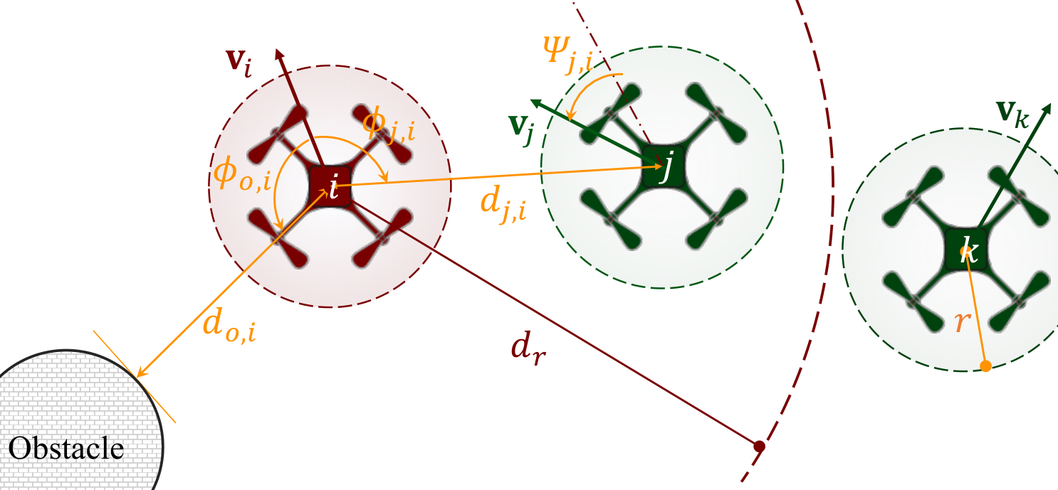
As shown in Fig. 2, all robots of interest in the environment are homogeneous, which has a safe radius of . Let be the distance from the robot to the surface of an obstacle, and be the distance between the robots and as in Fig. 2. Hence, collisions will occur if or . We use to denote the azimuth angle of an obstacle in the local frame of the robot as shown in Fig. 2. Similarly, is the azimuth angle of a robot in the local frame of the robot . The relative heading angle of a robot to robot is specified by . Assume that exteroceptive sensors are available for each robot to observe the environment, e.g., LiDAR or visual sensors. The detection or sensing range is represented by for each robot as illustrated in Fig. 2. Hence, based on the exteroceptive sensors, an robot is able to obtain all necessary environment states in its detection range for planning, including obstacle information {, } and neighouring robot information {, , }. The goal position for an robot is represented by , so . In summary, the objective of this paper is formulated as
| (2) |
III-B Reinforcement Learning
In RL, state transitions of environments are formulated as a Markov Decision Process (MDP) that is denoted by a tuple , where
- •
is the state space with denoting the environment state at the timestep .
- •
is the action space with being the action executed at the timestep .
- •
is the state-transition probability function.
- •
is the reward function;
- •
is a discount factor balancing the instant reward with future reward.
Let be the stochastic policy in RL with . The expectation of the accumulated reward is
| (3) |
where , , and is the task horizon. The objective of RL is to learn an optimal policy that maximizes the expectation of accumulated rewards in (3). The maximization problem can be resolved using diverse methods. In this paper, we adopt the well-known proximal policy optimization (PPO) algorithm [29]. Assume that the policy is approximated using a deep neural network with the parameter set , so the parameterized policy is denoted by . In PPO, the policy parameter is optimized by maximizing a surrogate objective as below. to limit the update of parameters into the trust region as follows [29].
| (4) |
where is the advantage function and is the clip parameter. More details can be found in [29].
III-C Artificial Potential Field
Artificial potential field methods guide robots to their predefined goals by the combination of multiple forces. The attractive force exerted on robot is defined as follows.
| (5) |
Accordingly, the repulsive force from an obstacle is
| (6) |
where is the scale factor. is the position of the nearest obstacle to robot . is the influence range of obstacles.
The inter-robot force that keeps robots away from each other is
| (7) |
where is the set of robots that can be detected by robot , namely , is a parameter adjusting the compactness of the multi-robot system. The smaller is, the more compact the system is [19]. The resultant force, therefore, is
| (8) |
The direction of is used as the commanded heading angle for robot .
IV Algorithm
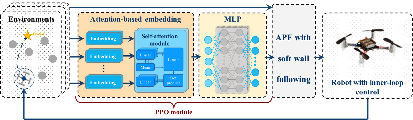
The reinforced potential field (RPF) algorithm proposed in this paper integrates attention-based embedding, PPO, and APF. Thereinto, the attention-based embedding transforms the observations into fixed-length vector according to the importance of neighboring robots and obstacles to the current decision-making process. Outputs of the attention-based embedding are fed into Multiple-Layer Perceptron (MLP) network to generate reasonable choices for a modified APF with a soft wall following mechanism. Therefore, we will describe the proposed algorithm from the aforementioned three aspects in this section.
IV-A Attention-based Embedding
In fully-connected neural networks, the input size is required to be fixed. However, in a multi-robot scenario, the number of neighbours of a robot would be dynamically changing, so it would be inefficient to use a fully-connected neural network to encode surrounding environments. To tackle this problem, the mean embedding methods are employed by averaging all the information of observed neighbors [30]. However, it is obvious that the information from different neighbors contributes differently to the current decision-making process in a sophisticated multi-robot systems, e.g., gregarious animals. However, the pure average in the mean embedding methods may underrate the information of a significant neighbor. Therefore, we introduce the self-attention mechanism into the observation embedding process in this paper to explicitly characterize the relative importance of surrounding observations, namely robot-robot interactions and robot-environment interactions.
The observations of each robot is firstly split to two parts, namely . The first part includes the relative distance and azimuth angles of the nearest obstacle and the goal information, so . The second part consists of the information of observed neighbors , where is
| (9) |
The attention-based embedding then employs two one-layer fully-connected networks to encode into two fixed-length high-dimensional vectors and , respectively. Both networks use ReLU activation functions.
| (10) | ||||
The attention score is calculated by inputting and the mean embedding of all observed neighbors into another one-layer fully-connected network. This network also uses ReLU activation functions.
| (11) |
where , where is the number of observed neighbors by a robot . The information of each observed neighbor is weighted according to their corresponding attention scores.
| (12) |
Finally, is concatenated with to represent the observations of robot with a fixed-length vector while highlighting the information from significant neighbors.
In the conventional artificial potential field methods, the scale factor in (6) determines the strength of obstacles’ influence, while in (7) adjusts the magnitude of individual force exerted from neighbors. Once these parameters are determined, they are invariant throughout the whole task. However, it is more promising to dynamically adjust these parameters online because their optimal values depend on the environment states in one episode. To encode the dynamic environment information into and , the outputs of the attention-based embedding will be fed into an MLP network. The whole framework will be optimized using PPO.
IV-B Optimization by PPO
The action space has two dimensions corresponding to and , respectively. The range of candidate action pairs is , which is empirically selected according to the specific scenarios used in Section V. All robots share the same policy network, so the same reward function is used for all robots. The total reward function for each robot is defined as
| (13) |
The reward encourages robots to reach their goals via the shortest trajectory. For a robot , one has
| (14) |
where is the Euclidean distance between the start point and the goal position, and denotes the trajectory length achieved by the robot .
The reward function encourages robots to move smoothly by giving a punishment of when the difference of headings at two adjacent timesteps exceeds .
The reward function is used to prevent robots from collisions with obstacles. For a robot , one has
| (15) |
The reward provides a dense reward to accelerate the learning process. For a robot , one has
| (16) |
where is the relative distance of the goal, and is a hyperparameter.
To extend the classical PPO algorithm to multi-robot settings, the parameter sharing technique is employed. That is, all robots share the same policy network. The shared policy network updates parameters using transitions collected by all robots. The overall procedure of the proposed algorithm is shown in Algorithm 1.
IV-C APF with soft wall following
Conventional artificial potential field method mentioned in Sec III-C can be stuck in a location, especially when and . In order to tackle this problem, our previous work introduced a wall following rule [19]. The wall-following rule means that when the agent is close to the obstacle, it should move along the edge of obstacles. As shown in Fig 4, or is the better direction for robots rather than . The wall following rule is activated when the angle between and exceeds .
The selection of and depends on the current heading direction and inter-robot force . If exceeds the specified a threshold , we select from and the one that has a smaller angle with as shown in Fig. 4 (a). Otherwise, choose the one with a smaller angle with the current motion direction as the robot in Fig. 4.
When the angle between and (or ) is very large, there might be a sharp turn as the blue trajectory shown in Fig. 4(b). To solve the problem, we introduce a soft rule to the wall following method. The nearby external area of an obstacle is divided into two sub-areas as shown in Fig. 4(b). In sub-area A, a robot chooses or according to the aforementioned wall following rule. In the sub-area B, the robot chooses a direction between and . Hence, is defined as
| (17) |
At the exact moment that a robot enters the sub-area B, is the same as . When agents get closer to obstacle, becomes closer to .
The sub-area A and B around an obstacle in Fig 4 are defined as follows: If , it belongs to sub-area A; if , it is in sub-area B.
| (18) |

| Parameters | Values |
|---|---|
| Initial learning rate | 0.0003 |
| 0.999 | |
| Actor neural network | MLP with 2 hidden layers |
| (256 neurons per hidden layer) | |
| Critic neural network | MLP with 2 hidden layers |
| (256 neurons per hidden layer) | |
| Sample batch size | 100 |
| PPO epochs | 1 |
| Training episodes | 1000 |
| Maximum steps per episode | 1000 |
| 0.9 | |
| 0.999 | |
| Clip parameter | 0.2 |
| 0.5 | |
| 0.001 |
V Simulation and experiments
In this section, numerical simulation and experimental results are presented. The proposed algorithm is trained in two different arenas with six robots as shown in Fig. 5. The trained results are thereafter evaluated in both numerical simulations with different setups and real-world experiments.
In the first arena, the environment is occupied with many obstacles as shown in Fig. 5 (a). The obstacles have the same radius of . Both the initial and goal positions of each robot are randomly given. All robots need to reach their goal positions, while avoiding collisions with each other and obstacles. The second training arena is shown in Figure 5 (b). It is an open environment with no obstacles. All robots need to avoid collisions with each other. Initially, all robots are distributed evenly on a circle with a radius of . The initial positions of all robots are randomly generated. Robots are required to swap their locations.
The same setup is chosen for the two aforementioned training arenas. Some training details are summarized in Table I. In the training, the desired speed of agents is set to . The safety radius of robots is . The perception range of a robot is chosen to be . The time step at training is set to be . The hyperparameter is chosen to be . The influence range of an obstacle is chosen . The wall following threshold is picked to be , . The learning rate decays as follows.
| (19) |
where is the initial learning rate, is a hyperparameter, and is the number of the current episode. The values of , are given in Table I.
The proposed RPF is compared with three different methods, namely RPF without attention, vanilla PPO, and vanilla APF. In the comparison, the proposed RPF in this paper is termed as “RPF 1”. When the attention module is replaced by pure linear embedding as in our previous work [19], we use the term “RPF 2” to represent it. The “RPF 2” algorithm is trained based on exactly the same reward functions with “RPF 1” using the same training setup.
For vanilla PPO, we found that it’s very difficult to train a policy in the cluttered environment shown in Fig 5 (a). For comparison, we train the vanilla PPO policy in an environment with smaller obstacles. The training environment would be easier than the one used in “RPF 1” and “RPF 2”. Hence, the radii of all obstacles are set to be . The locations of the obstacles are the same with those in Fig 5 (a). Other learning configurations are the same with those as “RPF 1” as given in table I. The decision of PPO robot is generated as follows.
| (20) |
where is a vector perpendicular to , and is the output by the PPO policy with .
We choose the parameters of a vanilla APF to be and . For a fair comparison, we choose two metrics to evaluate the performance of all methods in the simulation.
The traveling distance metric evaluates the average total traveling length by a robot, which is defined as below.
| (21) |
where represents the total timesteps for robots to reach their goal. The large the traveling distance metric is, the poor the algorithm’s performance is.
The motion smoothness metric evaluates how oscillatory the motion of a robot, which is defined as
| (22) |
Similarly, the large the motion smoothness metric is, the poor the performance of an algorithm is.
V-A Simulation Evaluation
In the simulation evaluation, the trained proposed algorithm is compared with the other three algorithms in three different scenarios to show its efficiency and generalization. In the first two scenarios, open environments with no obstacles are considered. In the second scenario, we built up a new evaluation arena with different obstacle distributions. All simulations and comparisons are given in Fig. 6 - 8. Both the traveling distance and motion smoothness metrics in Figs. 6 and 8 are averaged among all robots to evaluate the whole performance of the algorithms in a multi-robot setting.
In the first evaluation, we consider robots distributed on a circle with a radius of and swap locations with robots on the other side. This scenario is very similar to our second training arena but with a different number of robots and a different size of circle. The robot trajectories are shown in Fig. 6. In this scenario, PPO has the best performance in by both the traveling distance metric and the motion smoothness metric as shown in Fig. 6. The APF method has the worst performance by both metrics. The 1 (with the self-attention module) performs better than 1 (with no self-attention). It is that it is necessary to rank the importance of surrounding information.
Although the vanilla PPO has the best performance in the first scenario, it cannot generalize well to a scenario with more difference as shown in Figs. 7 and 8. In the second evaluation in Figs. 7, we further compare our method 1 with the vanilla PPO in a different scenaro. In this case, robots are initially distributed on a circle with a radius of that is large than the detection range ( ) of a robot. The same position swap task is performed. In such a scenario, the vanilla PPO failed to complete the task safely.
In the third scenario, we further evaluate the performance of all four algorithms in a different environment. In this scenario, the second robot collides with an obstacle, thus leading to a mission failure. Due to the mission failure of the second robot, the PPO algorithm has small values by both the distance metric and the motion smooth metric. In comparison with PPO, both 1 and 2 show better generalization, but 1 has much improvement by both the traveling distance and motion smoothness metrics. It further demonstrates the efficiency of the introduced attention-based observation embeddings.
V-B Experiment Evaluation

Experiment evaluation is performed to demonstrate the competence of the proposed algorithm in a real-life platform. A similar environment to the third simulation in Section V-A as shown in Fig 8. In the experiment, we apply the RPF 1 algorithm to Crazyflie quadrotors without any modification. The OptiTrack optical motion capture system is used to measure the states of quadrotors. The Crazyflie drones can track position commands from the high-level planner, using the implemented inner-loop controller.
Three different experiments are performed with a different number of robots as shown in Fig 9. A robot would change its trajectory if more robots are considered in the environment. The experiment also illustrates the generalization of the proposed algorithm to real-life systems.
VI Conclusion
Reinforced potential field, a novel motion planning algorithm integrating deep RL with APF, was presented in this paper. The proposed design was able to make active responses to dynamic changes in surrounding environments. An observation embedding with self-attention mechanism was developed to implicitly environment dynamic changes. A soft wall-following rule was presented to further improve the motion smoothness performance. The performance improvement of our algorithm over existing benchmarks, including PPO and APF, was demonstrated via numerical simulations. Real experiments were also performed to show the competence of the proposed method in real systems. In future works, we aim to integrate real sensor observations into our method for implementation in more diverse scenarios.
References
- [1] K. M. Wurm, C. Stachniss, and W. Burgard, “Coordinated multi-robot exploration using a segmentation of the environment,” in 2008 IEEE/RSJ International Conference on Intelligent Robots and Systems. Nice, France: IEEE, September 2008, pp. 4584–4589.
- [2] N. Mathew, S. L. Smith, and S. L. Waslander, “Planning paths for package delivery in heterogeneous multirobot teams,” IEEE Transactions on Automation Science and Engineering, vol. 12, no. 4, pp. 1298–1308, 2015.
- [3] L. Bai, J. Guan, X. Chen, J. Hou, and W. Duan, “An optional passive/active transformable wheel-legged mobility concept for search and rescue robots,” Robotics and Autonomous Systems, vol. 107, pp. 145–155, 2018.
- [4] M. Mohanan and A. Salgoankar, “A survey of robotic motion planning in dynamic environments,” Robotics and Autonomous Systems, vol. 100, pp. 171–185, 2018. [Online]. Available: https://www.sciencedirect.com/science/article/pii/S0921889017300313
- [5] J. Snape, J. Van Den Berg, S. J. Guy, and D. Manocha, “Smooth and collision-free navigation for multiple robots under differential-drive constraints,” in 2010 IEEE/RSJ international conference on intelligent robots and systems. Taipei, Taiwan: IEEE, 2010, pp. 4584–4589.
- [6] G. Zhao and M. Zhu, “Pareto optimal multi-robot motion planning,” in 2018 Annual American Control Conference (ACC), Milwaukee, WI, USA, 2018, pp. 4020–4025.
- [7] Y. F. Chen, M. Everett, M. Liu, and J. P. How, “Socially aware motion planning with deep reinforcement learning,” in 2017 IEEE/RSJ International Conference on Intelligent Robots and Systems (IROS). Vancouver, BC, Canada: IEEE, 2017, pp. 1343–1350.
- [8] H. Kretzschmar, M. Spies, C. Sprunk, and W. Burgard, “Socially compliant mobile robot navigation via inverse reinforcement learning,” The International Journal of Robotics Research, vol. 35, no. 11, pp. 1289–1307, 2016.
- [9] S. P. Chinchali, S. C. Livingston, M. Chen, and M. Pavone, “Multi-objective optimal control for proactive decision making with temporal logic models,” The International Journal of Robotics Research, vol. 38, no. 12-13, pp. 1490–1512, 2019.
- [10] J. Alonso-Mora, P. Beardsley, and R. Siegwart, “Cooperative collision avoidance for nonholonomic robots,” IEEE Transactions on Robotics, vol. 34, no. 2, pp. 404–420, 2018.
- [11] X.-T. Truong and T. D. Ngo, “Toward socially aware robot navigation in dynamic and crowded environments: A proactive social motion model,” IEEE Transactions on Automation Science and Engineering, vol. 14, no. 4, pp. 1743–1760, 2017.
- [12] M. Luber, L. Spinello, J. Silva, and K. O. Arras, “Socially-aware robot navigation: A learning approach,” in 2012 IEEE/RSJ International Conference on Intelligent Robots and Systems, Vilamoura-Algarve, Portugal, 2012, pp. 902–907.
- [13] H. Zhu and J. Alonso-Mora, “Chance-constrained collision avoidance for mavs in dynamic environments,” IEEE Robotics and Automation Letters, vol. 4, no. 2, pp. 776–783, 2019.
- [14] E. Soria, F. Schiano, and D. Floreano, “Predictive control of aerial swarms in cluttered environments,” Nature Machine Intelligence, vol. 3, no. 6, pp. 545–554, 2021.
- [15] O. Arslan and D. E. Koditschek, “Sensor-based reactive navigation in unknown convex sphere worlds,” The International Journal of Robotics Research, vol. 38, no. 2-3, pp. 196–223, 2019.
- [16] K. Cole and A. M. Wickenheiser, “Reactive trajectory generation for multiple vehicles in unknown environments with wind disturbances,” IEEE Transactions on Robotics, vol. 34, no. 5, pp. 1333–1348, 2018.
- [17] W. Yao, H. G. de Marina, B. Lin, and M. Cao, “Singularity-free guiding vector field for robot navigation,” IEEE Transactions on Robotics, vol. 37, no. 4, pp. 1206–1221, 2021.
- [18] D. Panagou, “Motion planning and collision avoidance using navigation vector fields,” in 2014 IEEE International Conference on Robotics and Automation (ICRA). Hong Kong, China: IEEE, 2014, pp. 2513–2518.
- [19] Z. Zhang, X. Wang, Q. Zhang, and T. Hu, “Multi-robot cooperative pursuit via potential field-enhanced reinforcement learning,” in 2022 International Conference on Robotics and Automation (ICRA), Philadelphia, PA, USA, 2022, pp. 8808–8814.
- [20] C. Y. Tan, S. Huang, K. K. Tan, and R. S. H. Teo, “Three dimensional collision avoidance for multi unmanned aerial vehicles using velocity obstacle,” Journal of Intelligent & Robotic Systems, vol. 97, pp. 227–248, 2020.
- [21] R. Tallamraju, S. Rajappa, M. J. Black, K. Karlapalem, and A. Ahmad, “Decentralized mpc based obstacle avoidance for multi-robot target tracking scenarios,” in 2018 IEEE International Symposium on Safety, Security, and Rescue Robotics (SSRR), Philadelphia, PA, USA, 2018, pp. 1–8.
- [22] M. Aoki, K. Honda, H. Okuda, T. Suzuki, A. Ito, and D. Nagasaka, “Obstacle avoidance control based on nonlinear mpc for all wheel driven in-wheel ev in steering failure,” in 2022 IEEE 25th International Conference on Intelligent Transportation Systems (ITSC), Macau, China, 2022, pp. 2863–2868.
- [23] O. Khatib, “Real-time obstacle avoidance for manipulators and mobile robots,” in Proceedings. 1985 IEEE International Conference on Robotics and Automation, vol. 2, 1985, pp. 500–505.
- [24] S. S. Ge and Y. J. Cui, “Dynamic motion planning for mobile robots using potential field method,” Autonomous robots, vol. 13, pp. 207–222, 2002.
- [25] B. Riviere, W. Hönig, Y. Yue, and S.-J. Chung, “Glas: Global-to-local safe autonomy synthesis for multi-robot motion planning with end-to-end learning,” IEEE robotics and automation letters, vol. 5, no. 3, pp. 4249–4256, 2020.
- [26] C. Chen, Y. Liu, S. Kreiss, and A. Alahi, “Crowd-robot interaction: Crowd-aware robot navigation with attention-based deep reinforcement learning,” in 2019 international conference on robotics and automation (ICRA). Montreal, QC, Canada: IEEE, 2019, pp. 6015–6022.
- [27] T. Fan, P. Long, W. Liu, and J. Pan, “Distributed multi-robot collision avoidance via deep reinforcement learning for navigation in complex scenarios,” The International Journal of Robotics Research, vol. 39, no. 7, pp. 856–892, 2020.
- [28] S. H. Semnani, H. Liu, M. Everett, A. de Ruiter, and J. P. How, “Multi-agent motion planning for dense and dynamic environments via deep reinforcement learning,” IEEE Robotics and Automation Letters, vol. 5, no. 2, pp. 3221–3226, 2020.
- [29] J. Schulman, F. Wolski, P. Dhariwal, A. Radford, and O. Klimov, “Proximal policy optimization algorithms,” arXiv preprint arXiv:1707.06347, 2017.
- [30] M. Hüttenrauch, S. Adrian, G. Neumann et al., “Deep reinforcement learning for swarm systems,” Journal of Machine Learning Research, vol. 20, no. 54, pp. 1–31, 2019.