Formal Verification of Robotic Contact Tasks via Reachability Analysis^footnoteinfoThis work has been supported by Siemens AG.

We denote vectors by bold lowercases (e.g., $\bm{a}$), matrices by bold uppercases (e.g., $\bm{A}$), lists by sans-serif font (e.g., $\mathsf{A}$), and sets by calligraphic font (e.g., $\mathcal{A}$). Sets in this work are represented mainly by zonotopes (Kühn 1998):

On zonotopes, many operations can be exactly and efficiently computed (Althoff et al. 2021), such as Minkowski addition $\mathcal{A}\oplus\mathcal{B}:=\left\{\bm{a}+\bm{b}\,\middle|\,\bm{a}\in\mathcal{A},\bm{b}\in\mathcal{B}\right\}$ and linear transformation $\bm{M}\otimes\mathcal{A}:=\left\{\bm{M}\bm{a}\,\middle|\,\bm{a}\in\mathcal{A}\right\}$. To evaluate the volume of a zonotope, we use the $n^{th}$ root of its interval-hull volume (Kühn 1998).

Contact tasks are formalized as hybrid automata, with a definition similar to Kochdumper and Althoff 2020:

We consider urgent transition semantics (Henzinger and Ho 1995) and define guards as hyperplanes. The evolution of a hybrid automaton is illustrated in Fig. 2 and is informally described as follows: Starting from an initial location $L^{0}$ with initial continuous state $\bm{x}^{0}\in\mathcal{X}^{0}$, $\bm{x}(t)$ evolves following the flow function of $L^{0}$. When $\bm{x}(t)$ hits the guard set of a transition, the state transits to the corresponding target location in zero time. In case several guard sets are hit at the same time, the transition is chosen non-deterministically. After a transition, the continuous state is updated by the jump function and the result becomes the initial state in the new location where the evolution continues. We denote the trajectory of the continuous state for the evolution described above by $\xi(t,L^{0},\bm{x}^{0},\bm{u}(\cdot))$, where $\bm{u}(\cdot)$ is an input trajectory.

We are interested in the continuous reachable set of hybrid automata (Kochdumper and Althoff 2020):

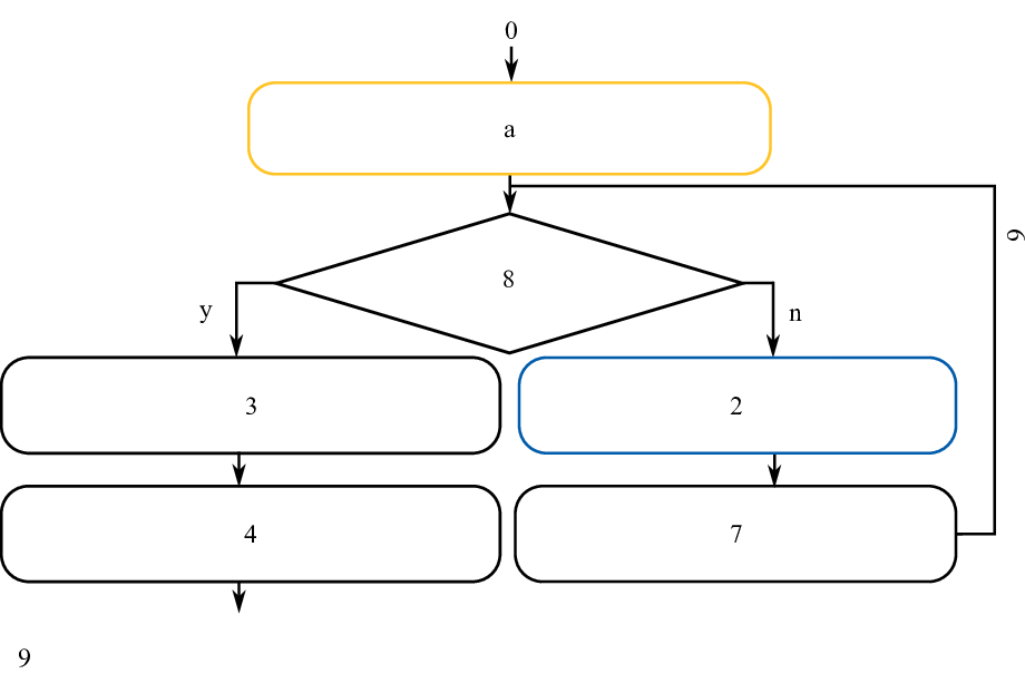
Since the exact reachable set $\mathcal{R}^{e}(t)$ can only be computed for a limited class of hybrid automata (Lafferriere et al. 1999), we compute tight over-approximations $\mathcal{R}(t)\supset\mathcal{R}^{e}(t)$. The computation for all times $[0,t_{f}]$ is simply the union of the reachable sets of subsequent time intervals. Accordingly, we compute $\mathcal{R}_{0,1},\ldots,\mathcal{R}_{N-1,N},N\in\mathbb{N}$ such that $\mathcal{R}_{k,k+1}\supset\mathcal{R}^{e}([k\Delta\tau,(k+1)\Delta\tau])$, where the time step size $\Delta\tau=t_{f}/N$ is a tunable parameter largely influencing the computation accuracy (Wetzlinger et al. 2020). The basic procedure of computation is shown in Fig. 4 in black boxes, which repeats in each location:

1. 1.

   Starting from the initial set, compute the reachable sets of subsequent time intervals $\mathcal{R}_{k,k+1}$ until the reachable set $\mathcal{R}_{k}$ of time point $k\Delta\tau$ leaves the invariant or the time horizon $t_{f}$ is reached.

2. 2.

   When the reachable sets intersect a guard set $\mathcal{G}_{j}$ from time $t_{h}$ to $t_{l}$ (bounded in this work), compute the intersection $\mathcal{I}_{j}$ of $\mathcal{R}([t_{h},t_{l}])$ with $\mathcal{G}_{j}$. When multiple guard sets (e.g., $\mathcal{G}_{1},\mathcal{G}_{2}$) are hit by the reachable sets, separately compute $\mathcal{I}_{1}$ and $\mathcal{I}_{2}$, as illustrated by the yellow sets in Fig. 2. In that case, the intersection $\mathcal{I}_{j}$ can be tightened by removing the parts which trigger other transitions before intersecting $\mathcal{G}_{j}$, resulting in the green sets in Fig. 2. In this work, the pruning can be realized by intersecting $\mathcal{I}_{j}$ with the invariant.

3. 3.

   For each intersected guard, propagate the intersection using the jump function, the result of which becomes the initial set in the target location.

The input in a robot task commonly contains a user-specified discrete-time trajectory $\mathsf{U}_{d}=(\bm{u}_{d,0},\ldots,\bm{u}_{d,f})$, where $f$ denotes the final step. Given a trajectory sampled at time points $t_{k}=kT,k\in\mathbb{N}_{0}$ with time increment $T\in\mathbb{R}_{>0}$, the continuous-time input is realized by zero-order hold as

The above input requires that the propagation of reachable sets is synchronized with time—this has not yet been realized for hybrid systems so far, because time synchronization is not maintained after guard intersections as will be detailed later.

We verify the robot behavior in contact tasks modeled as hybrid automata. Given an initial location $L^{0}$, an initial set $\mathcal{X}^{0}$, an input set $\mathcal{U}=f^{u}(\bm{u}_{d}(t),\mathcal{U}_{u})$ with a discrete-time input trajectory $\bm{u}_{d}$ as well as an uncertainty set $\mathcal{U}_{u}$, and an unsafe set $\mathcal{F}$ representing the violation of task specifications, the verification problem for a time interval $[0,t_{f}]$ is:

By using reachability, we can verify safety as follows:

A robotic system typically consists of the robot itself and its controller. We denote the variables associated with the robot by superscript $r$ and the variables associated with the controller by superscript $c$. For the system in Fig. 1, the controller uses $\bm{x}_{f}^{c}=\begin{bmatrix}{\bm{z}^{c}}&{\bm{\dot{z}}^{c}}\end{bmatrix}$ which is the delayed measurement of the system states $\bm{x}_{f}^{r}=\begin{bmatrix}{\bm{z}^{r}}&{\bm{\dot{z}}^{r}}\end{bmatrix}$, where $\bm{z}^{r}\in\mathbb{R}^{6}$ is the position of the tool center point (TCP). The user-specified input trajectory is $\bm{u}_{d}=\begin{bmatrix}\bm{z}_{d}&\dot{\bm{z}}_{d}&\ddot{\bm{z}}_{d}\end{bmatrix}$, where $\bm{z}_{d},\dot{\bm{z}}_{d},\ddot{\bm{z}}_{d}\in\mathbb{R}^{6}$ are respectively the desired position, velocity, and acceleration for the TCP.

The robot dynamics in Cartesian coordinates is the result of actuation force $\bm{f}_{\tau}^{r}$ and contact force $\bm{f}_{e}^{r}$ applied to the effective mass $\bm{\Lambda}(\bm{q})$ (Khatib 1995, eq. 6), which depends on the joint position vector $\bm{q}$:

We only consider nonsingular configurations of robots and the translational part of the dynamics, since our main interest is in the normal force. Assuming that the posture of robots barely changes during contact, the effective mass of the robot along one direction can be approximated by a constant value $m$ (Khatib 1995). Accordingly, the three Cartesian dimensions can be decoupled, leading to a scalar representation of the dynamics in the normal-force direction:

Two typical modes are considered for the robot controller: One mode is a Cartesian impedance controller (Albu-Schäffer et al. 2003, eq. 19), with desired stiffness and damping factors $k_{t},d_{t}$:

The other mode is a collision reaction mode (De Luca and Flacco 2012) with damping factor $d_{r}$, which is triggered once the controller receives a contact force ${f}^{c}_{e}$ exceeding the user-defined threshold ${f}_{t}$:

To model the contact force ${f}_{e}^{r}$, we adopt the widely used Kelvin-Voigt contact model (Achhammer et al. 2010), as it provides reasonable results for most cases despite its simplicity (Gilardi and Sharf 2002). Given $l$ as the radius of the sphere in Fig. 1, $k_{e},d_{e}$ respectively as the stiffness and damping coefficients of the contact, we have:

With (3)-(6), we obtain the system dynamics in the direction of the normal force. Please note that the one-dimensional abstraction is commonly used in relevant studies (Muradore et al. 2011; Liu and Althoff 2021; Achhammer et al. 2010, e.g.,). Despite its simplicity, it is proven sufficient in describing higher-dimensional cases when the nonlinear dynamics are decoupled and compensated for (Niculescu and Brogliato 1999).

We consider two crucial time delays in the system: a robot-to-controller delay $d_{rc}$ and a controller-to-robot delay $d_{cr}$. The input is only affected by $d_{cr}$, while the state is affected by both delays. Accordingly, the actual actuation force at time $t$ is:

where the delays are rewritten as $d_{1},d_{2}$, and the delayed variables are denoted by a hat.

While the delayed input $\hat{\bm{u}}_{d}$ can be easily obtained with a predefined input trajectory, we approximate the delay differential equation of states $\dot{\hat{\bm{x}}}_{f}^{r}(t)=\dot{{\bm{x}}}_{f}^{r}(t-d_{2})$ using the Padé approximation (Moler and Van Loan 2003) to employ powerful methods for the reachability analysis of ordinary differential equations. Because the time delay is rather short in modern robotic systems and to avoid numerous additional state variables (reduces the computation time of reachability analysis), we employ a Padé approximation of first-order:

We model the overall system using a hybrid automaton as shown in Fig. 3. The discrete state transits to $L_{2}$ from $L_{1}$ if the robot approaches the surface and transits back to $L_{1}$ when the robot leaves the surface. If the delayed contact force $\hat{f}_{e}^{r}(t)=-k_{e}\hat{z}^{r}-d_{e}\hat{\dot{z}}^{r}$ breaches the threshold $f_{t}$, the collision reaction is triggered (transition from $L_{2}$ to $L_{3}$) to decrease the potential damage. The control mode stays in collision reaction since then, and the transitions between $L_{3}$ and $L_{4}$ are similar to those between $L_{1}$ and $L_{2}$. The task can be reset by user input, as illustrated by the dotted arrow in Fig. 3.

The state-space model of the system is defined given the state vector $\bm{x}=\begin{bmatrix}\bm{x}^{r}_{f}&\bm{\hat{x}}^{r}_{f}&t\end{bmatrix}^{\mathsf{T}}=\begin{bmatrix}z^{r}&\dot{z}^{r}&\hat{z}^{r}&\hat{\dot{z}}^{r}&t\end{bmatrix}^{\mathsf{T}}$, and the input vector $\bm{u}=\hat{\bm{u}}_{d}{}^{\mathsf{T}}=\begin{bmatrix}\hat{z}_{d}&\hat{\dot{z}}_{d}&\hat{\ddot{z}}_{d}\end{bmatrix}^{\mathsf{T}}$. The state variable $t$ serves as a clock. Having a clock associated to the state allows us to track the time by projecting a state vector to time (operator $\text{\tt{proj}}_{t}$):

which will be used in Sec. 4.1 to address the time synchronization problem mentioned in Sec. 2.1. Accordingly, the flow function is obtained as

The first line, i.e., $\dot{\bm{x}}_{f}^{r}=\left[\begin{array}[]{@{}*{3}{c}@{}}\bm{A}_{1}&\bm{A}_{2}\end{array}\right]\,\left[\begin{array}[]{@{}*{3}{c}@{}}\bm{x}^{r}_{f}&\bm{\hat{x}}^{r}_{f}\end{array}\right]^{\mathsf{T}}+\bm{B}_{1}\bm{\hat{u}}_{d}{}^{\mathsf{T}}$, represents the robot dynamics, where the values in the matrices vary for each location and can be easily derived from (3)-(7). The second line is simply the delay formulation (8), and the third line models the clock.

In Sec. 2.1, we explained the basic procedure for the reachability analysis of hybrid systems with the input set $\mathcal{U}$ given, and proposed (1) to extract the input from a discrete-time trajectory based on time $t$. However, set propagations are not synchronized with the discretized time $k\Delta\tau$ after guard intersection, which unifies the sets of states that hit the guard at different times and thus introduces time uncertainty. Accordingly, we associate a clock with the state, as illustrated in Sec. 3.3, and introduce two additional steps below for reachability analysis with discrete-time input trajectories.

To precisely enclose the possible inputs for each iteration, we introduce the step in the blue box in Fig. 4. At the beginning of iteration $k$, we compute the time interval associated with $\mathcal{R}_{k,k+1}$ to capture the time uncertainty introduced by guard intersection:

We enclose the discrete-time inputs during the time interval $\mathcal{T}$ by a zonotope. For the system modeled in Sec. 3, the enclosure is computed as

where the input uncertainty $\mathcal{U}_{u}\subset\mathbb{R}^{3}$ is represented by a zonotope.

Obviously, the time uncertainty enlarges the input set $\mathcal{U}$ in (11) and causes unnecessary over-approximation. To address this, we remove the time uncertainty using the step in the yellow box in Fig. 4. When the state enters a location after intersection (intersection set $\mathcal{I}$), we compute the start and the end of the intersection period $t_{h},t_{l}$ as the infimum and supremum of $\text{\tt{proj}}_{t}(\mathcal{I})$. Then, we compute the set propagations for a period of $t_{l}-t_{h}$ with a time step size $\Delta\tau=(t_{l}-t_{h})/N$ and obtain the reachable set $\mathcal{R}_{0,N}$. The set $\mathcal{R}_{0,N}$ contains all the states reachable at $t_{l}$ in the current location, and thus we can compute $\mathcal{R}(t_{l})$ as

By taking $\mathcal{R}(t_{l})$ as the initial set, the subsequent set propagations are time synchronized. We apply the introduced technique selectively by checking the magnitude of $t_{l}-t_{h}$ a priori.

The idea of our novel guard-intersection approach is intuitive: we select and combine complementary approaches that are scalable with the system dimension. Three approaches are adopted: hyperplane mapping (Althoff and Krogh 2012), dynamics scaling (Bak et al. 2017), and an efficient geometric approach implemented in CORA (Althoff 2015).

We first recall the three relevant approaches. The geometric approach represents all the sets intersecting the guard $\mathcal{P}_{1},\ldots,\mathcal{P}_{p}$ by constrained zonotopes (Scott et al. 2016), which are closed under intersection with hyperplanes. Then the intersections between $\mathcal{P}_{i}$ and the guard set $\mathcal{G}$ are enclosed by their interval hulls for efficiently computing their union:

The operator intervalHull computes the tightest interval enclosure of a constrained zonotope by solving $2n$ linear programs, which determines the computational complexity of the geometric approach. A trade-off between accuracy and scalability usually has to be found for geometric approaches. The above method is designed to sacrifice accuracy for efficiency; due to the strong dependencies between states in contact dynamics, accurate geometric intersection would be costly.

In contrast to geometric intersection, the mapping method can tightly enclose guard intersection despite good scalability with complexity $\mathcal{O}(n^{6})$ (Althoff and Krogh 2012, p. 2). The mapping method abstracts a system to a state-dependent constant flow $\dot{\bm{x}}=\bm{A}\bm{x}^{0}+\bm{b}$, where $\bm{x}^{0}$ is the initial state, $\bm{A}$ is the system matrix, and $\bm{b}$ is a constant vector. For a transition happening in $[t_{h},t_{l}]$, the intersection is enclosed by bounding the constant-flow evolution with an abstraction-error set $\mathcal{E}$:

The accuracy of the approach highly depends on the duration from the first to the last intersection of the reachable set with the guard set; $\mathcal{E}$ is large if the time interval $[t_{h},t_{l}]$ is long.

The dynamics scaling approach is another way to avoid geometric intersection operations, which introduces a scaling phase before the intersection with the dynamics scaled as $f^{s}(\bm{x},\bm{u})=g(\bm{x})f(\bm{x},\bm{u})$. The scaling function $g(\bm{x})$ is defined to flatten the set of states against the guard hyperplane during continuous evolution; the flattened set $\mathcal{R}^{s}_{h}$ crosses the guard within a short period $[t_{h}^{s},t_{l}^{s}]$, and thus the intersection can be tightly enclosed by $\mathcal{R}([t_{h}^{s},t_{l}^{s}])$. Due to the nonlinearity introduced by the scaling function, the scaling phase basically reduces to the reachability analysis for nonlinear dynamics with complexity $\mathcal{O}(n^{5})$ (Althoff 2013, Sec. 5); the nonlinear dynamics leads to a large over-approximation in $\mathcal{R}^{s}_{h}$ if it takes long to flatten the set.

We combine the three approaches to compensate for their individual shortcomings, as shown in Fig. 5: We use the scaling approach to flatten the set as the blue sets show, then map the flattened set $\mathcal{R}^{s}_{h}$ to the guard hyperplane using the mapping method as presented by the yellow arrow. The scaling phase shortens the duration of the intersection for the mapping method, while the latter allows terminating the scaling phase before the set expands too much. We refer to the above combination as time-scaling-mapping (TSM), whose result is denoted by $\mathcal{I}_{tsm}$. Meanwhile, we compute the geometric intersection $\mathcal{I}_{g}$ and combine the result to $\mathcal{I}_{t}:=\mathcal{I}_{g}\cap\mathcal{I}_{tsm}$; the resulting method is referred to as trinal intersection.

Additionally, we introduce two measures to determine when to terminate the scaling phase for TSM. The first measure evaluates whether the intersection duration is short enough by estimating the time required by a set $\mathcal{X}$ to cross a guard hyperplane $\mathcal{G}:=\left\{\bm{x}\,\middle|\,\bm{c}^{\mathsf{T}}\bm{x}=d\right\},\|\bm{c}\|=1$, given the center of the input set $\bm{u}_{c}$:

where $\delta$ represents the length of the set towards the normal direction of the hyperplane while ${\text{\tt{dist}}}(\mathcal{X},\mathcal{G})$ returns the possible distances from states $\bm{x}\in\mathcal{X}$ to hyperplane $\mathcal{G}$ as an interval; the denominator approximates the traversing speed by projecting the flow of the center point $\dot{\bm{x}}_{c}$ onto the normal direction of the hyperplane. The second measure evaluates the expansion of the reachable set to limit the over-approximation in the guard intersection, for which sets are projected onto a plane perpendicular to the flow:

where vol returns the volume of the projected set, and $\mathcal{R}_{h}$ is the initial set of the scaling phase.

The implementation of our trinal approach is presented in Alg. 1, involving the following steps (the line numbers coincide with the steps):

1. 1.

   Obtain scaled system dynamics $f^{s}(\bm{x},\bm{u})$, with scaling function $g(\bm{x})=k_{s}\text{\tt{dist}}(\bm{x},\mathcal{G})/\mathrm{sup}(\text{\tt{dist}}(\mathcal{R}_{h},\mathcal{G}))$, where $k_{s}$ is a gain for tuning.

2. 2.

   Obtain a flattened set $\mathcal{R}^{s}_{h}$ through a scaling phase, where the operator reachUntil computes the reachable sets of the scaled dynamics starting from $\mathcal{R}_{h}$ until $r^{\delta}$ decreases to the desired threshold $r^{\delta}_{d}$ or $r^{v}$ reaches its limit $r^{v}_{d}$.

3. 3.

   Operation refine computes the reachable sets starting from $\mathcal{R}^{s}_{h}$ with a finer time step size until the set leaves the invariant, in order to refine the list of reachable sets $\mathcal{P}_{1}^{s},\ldots,\mathcal{P}_{q}^{s}$ that intersect the guard. An approximative intersection duration ${T^{s}}$ is obtained as the duration between the first step intersecting the guard and the first step after leaving the invariant.

4. 4.

   Operation input extracts the input set involved in the intersection, using (1) and (11) where the time interval is $[\mathrm{inf}(\text{\tt{proj}}_{t}(\mathcal{P}_{1}^{s})),\mathrm{sup}(\text{\tt{proj}}_{t}(\mathcal{P}_{q}^{s}))]$.

5. 5.

   Map $\mathcal{R}^{s}_{h}$ to the hyperplane using the mapping method (operation map) to obtain the result of the TSM approach $\mathcal{I}_{tsm}$.

Meanwhile, we compute the geometric intersection $\mathcal{I}_{g}$. The final result $\mathcal{I}_{tsm}\cap\mathcal{I}_{g}$ can be efficiently computed by enclosing zonotopes by their interval hulls.

The parameters of the system in Sec. 3 are listed in Tab. 1. Three cases of effective mass are considered, according to the mass distribution of typical robots (Kirschner et al. 2021b). The controller gains in task execution are adopted from the work of DLR (Albu-Schäffer et al. 2003, p. 4), and the damping factor is defined as $d_{t}=2\sqrt{mk_{t}}$. For the collision reaction mechanism, the damping factor is tuned by the authors, and the force threshold of $100\text{\,}\mathrm{N}$ is a typical value of robots in the market (Kirschner et al. 2021a). Regarding the contact dynamics, we simplify the sphere to a point mass as its geometry does not affect the system behavior. The contact coefficients are defined to represent human hands as in ISO/TS 15066 (ISO 2016). Time delays are quantified based on the controller cycle time $T_{c}$ and servo cycle time $T_{s}$ of DLR LWR III (Albu-Schäffer et al. 2007) with approximations ${d_{rc}\approx 2T_{s}\approx 0.0006,d_{cr}\approx T_{c}+T_{s}\approx 0.0013}$.

The discrete-time input $\bm{u}_{d,k}$ is defined as a list of trajectory points sampled at $1\text{\,}\mathrm{[}$]kHz, which hits the surface at $0.1\text{\,}\mathrm{[}$] with speed $v$ and stops at $z_{d}=-0.06$, and a zonotope $([0\mkern 5.0mu0\mkern 5.0mu0]^{\mathsf{T}},[0.00005\mkern 5.0mu0\mkern 5.0mu0]^{\mathsf{T}})$ following Def. 1 describes the input uncertainty $\mathcal{U}_{u}$ due to the uncertainties in the reference frame. The initial set of states is represented by a zonotope $(\bm{u}_{d,0},\text{\tt{diag}}([0.0001\mkern 5.0mu0.002\mkern 5.0mu0.0001\mkern 5.0mu0.002\mkern 5.0mu0]^{\mathsf{T}}))$, where the operator diag returns a diagonal matrix with the vector elements on the main diagonal. The time step size $\Delta\tau$ is $6.5\text{\times}{10}^{-4}\text{\,}\mathrm{[}$], which is derived from half of the delay $d_{cr}$ to avoid large errors in the delayed states.

We analyze the system for $0.8\text{\,}\mathrm{[}$]s in 15 cases obtained by combining three effective masses (1.5, 4.5, 8 $\text{\,}\mathrm{[}$]kg) and five collision speeds (0.1, 0.2, 0.35, 0.45, 0.55 $\text{\,}\mathrm{[}$]m/s). The contact force can be easily obtained as described in (6) using the linear transformation of zonotopes; the results are shown in Fig. 6, which presents very similar behaviors with regard to the experimental results in Kirschner et al. 2021a: Both the robot mass and the collision speed have a positive correlation with the contact force reached. If the threshold of $100\text{\,}\mathrm{[}$]N is not met, the robot tends to stay in contact with the surface, which is the case for low collision speeds such as the purple sets. When the collision reaction is triggered, the contact force decreases to zero; the robot leaves the surface due to the contact force and stops. The dotted lines in Fig. 6 represent the safety limits for human hands (Kirschner et al. 2021a): $280\text{\,}\mathrm{[}$]N for transient contact (0 to $0.5\text{\,}\mathrm{[}$]s of the contact) and $120\text{\,}\mathrm{[}$]N for quasi-static contact (after $0.5\text{\,}\mathrm{[}$]s), hence the states with an $f_{e}^{r}$ above the limits form an unsafe set $\mathcal{F}$. By checking whether the reachable sets intersect the thresholds, we can easily verify whether a robot is safe for HRI under a certain speed, and thus define the permissible speed of the robot or fine-tune the controllers. The verification obviously benefits from the accuracy of guard intersection: $m=4.5,v=0.55$ can be verified as safe by our trinal approach, while the geometric approach is not able to verify its safety.

With case $m=8,v=0.1$ we demonstrate the effect of the technique introduced in Sec. 4.1, which removes the time uncertainty after guard intersection. The boundaries of the resulting reachable sets are plotted in pink in Fig. 6. It can be seen that the additional operation leads to more conservative results for the approximately $0.05\text{\,}\mathrm{[}$]s after the intersection due to a larger initial set, while a better accuracy can be observed in the long term due to a smaller input uncertainty. In practice, the verification can be more accurate using both results: Since all possible states are enclosed by their intersection, the specifications are violated only if both results intersect the unsafe set.

We evaluate the accuracy of the proposed guard intersection approaches in comparison with the three methods illustrated in Sec. 4.2: mapping, scaling, and geometric intersection. As shown in Tab. 3, TSM shows a clear improvement compared to mapping and scaling. It also shows overall better accuracy compared to the geometric approach. Using the latter, the set volume grows significantly during the transition from $L_{2}$ to $L_{3}$ due to the over-approximation in the reachable sets of time intervals; as a result, the geometric approach fails with $m=1.5,v=0.35,0.45,0.55$ where the contact force leads to high acceleration $\ddot{z}^{r}$. However, TSM is inaccurate with low-speed collisions ($v=0.1$), where the algorithm cannot effectively shorten the intersection duration, and manual fine-tuning of the scaling function may help. The proposed trinal intersection accomplishes all cases and shows the best accuracy among the tested methods. It can be seen that, for the trinal approach, TSM determines the final result with good accuracy in most cases, while the intersection with $\mathcal{I}_{g}$ provides a usable result even if the intersection duration cannot be effectively shortened before the reachable set overexpands.

The computation times of guard intersections are shown in Tab. 3. For better readability, we average the time consumed in the runs where all methods pass. The proposed approaches are significantly more efficient than the scaling approach because the mapping method and the measures introduced in Sec. 4.2 realize a shorter scaling phase, and the accuracy is even improved due to a tighter flattened set. The complexity of the two proposed approaches is determined by the mapping method with $\mathcal{O}(n^{6})$, which indicates good scalability.

References

- Achhammer et al. (2010) Achhammer, A., Weber, C., Peer, A., and Buss, M. (2010). Improvement of model-mediated teleoperation using a new hybrid environment estimation technique. In Proc. of the 2010 IEEE International Conference on Robotics and Automation, 5358–5363.
- Ajoudani et al. (2018) Ajoudani, A., Zanchettin, A.M., Ivaldi, S., Albu-Schäffer, A., Kosuge, K., and Khatib, O. (2018). Progress and prospects of the human–robot collaboration. Autonomous Robots, 42(5), 957–975.
- Albu-Schäffer et al. (2007) Albu-Schäffer, A., Haddadin, S., Ott, C., Stemmer, A., Wimböck, T., and Hirzinger, G. (2007). The DLR lightweight robot: Design and control concepts for robots in human environments. Industrial Robot: An International Journal, 34(5), 376–385.
- Albu-Schäffer et al. (2003) Albu-Schäffer, A., Ott, C., Frese, U., and Hirzinger, G. (2003). Cartesian impedance control of redundant robots: Recent results with the DLR-light-weight-arms. In Proc. of the 2003 IEEE International Conference on Robotics and Automation, volume 3, 3704–3709.
- Althoff (2013) Althoff, M. (2013). Reachability analysis of nonlinear systems using conservative polynomialization and non-convex sets. In Proc. of the 16th International Conference on Hybrid Systems: Computation and Control, 173–182.
- Althoff (2015) Althoff, M. (2015). An introduction to CORA 2015. In ARCH14-15. 1st and 2nd International Workshop on Applied Verification for Continuous and Hybrid Systems, volume 34, 120–151.
- Althoff et al. (2021) Althoff, M., Frehse, G., and Girard, A. (2021). Set propagation techniques for reachability analysis. Annual Review of Control, Robotics, and Autonomous Systems, 4(1), 369–395.
- Althoff and Krogh (2011) Althoff, M. and Krogh, B.H. (2011). Zonotope bundles for the efficient computation of reachable sets. In Proc. of the IEEE Conference on Decision and Control and European Control Conference, 6814–6821.
- Althoff and Krogh (2012) Althoff, M. and Krogh, B.H. (2012). Avoiding geometric intersection operations in reachability analysis of hybrid systems. In Proc. of the 15th ACM International Conference on Hybrid Systems: Computation and Control, 45–54.
- Althoff et al. (2010) Althoff, M., Stursberg, O., and Buss, M. (2010). Computing reachable sets of hybrid systems using a combination of zonotopes and polytopes. Nonlinear Analysis: Hybrid Systems, 4(2), 233–249.
- Bak et al. (2017) Bak, S., Bogomolov, S., and Althoff, M. (2017). Time-triggered conversion of guards for reachability analysis of hybrid automata. In International Conference on Formal Modeling and Analysis of Timed Systems, 133–150.
- Bresolin et al. (2012) Bresolin, D., Di Guglielmo, L., Geretti, L., Muradore, R., Fiorini, P., and Villa, T. (2012). Open problems in verification and refinement of autonomous robotic systems. In Proc. of the 2012 15th Euromicro Conference on Digital System Design, 469–476.
- De Luca and Flacco (2012) De Luca, A. and Flacco, F. (2012). Integrated control for pHRI: Collision avoidance, detection, reaction and collaboration. In 2012 4th IEEE RAS & EMBS International Conference on Biomedical Robotics and Biomechatronics, 288–295.
- Gilardi and Sharf (2002) Gilardi, G. and Sharf, I. (2002). Literature survey of contact dynamics modelling. Mechanism and Machine Theory, 37(10), 1213–1239.
- Girard and Le Guernic (2008) Girard, A. and Le Guernic, C. (2008). Zonotope/hyperplane intersection for hybrid systems reachability analysis. In Hybrid Systems: Computation and Control, volume 4981, 215–228.
- Haddadin et al. (2008) Haddadin, S., Albu-Schäffer, A., Frommberger, M., and Hirzinger, G. (2008). The role of the robot mass and velocity in physical human-robot interaction - Part II: Constrained blunt impacts. In 2008 IEEE International Conference on Robotics and Automation, 1339–1345.
- Henzinger and Ho (1995) Henzinger, T.A. and Ho, P.H. (1995). HyTech: The Cornell hybrid technology tool. In Hybrid Systems II, Lecture Notes in Computer Science, 265–293.
- ISO (2016) ISO (2016). ISO/TS 15066:2016: Robots and robotic devices — Collaborative robots.
- Khatib (1995) Khatib, O. (1995). Inertial properties in robotic manipulation: An object-level framework. The International Journal of Robotics Research, 14(1), 19–36.
- Kirschner et al. (2021a) Kirschner, R.J., Mansfeld, N., Abdolshah, S., and Haddadin, S. (2021a). Experimental analysis of impact forces in constrained collisions according to ISO/TS 15066. In Proc. of the 2021 IEEE International Conference on Intelligence and Safety for Robotics, 1–5.
- Kirschner et al. (2021b) Kirschner, R.J., Mansfeld, N., Pena, G.G., Abdolshah, S., and Haddadin, S. (2021b). Notion on the correct use of the robot effective mass in the safety context and comments on ISO/TS 15066. In Proc. of the 2021 IEEE International Conference on Intelligence and Safety for Robotics, 6–9.
- Kochdumper and Althoff (2020) Kochdumper, N. and Althoff, M. (2020). Reachability analysis for hybrid systems with nonlinear guard sets. In Proc. of the 23rd International Conference on Hybrid Systems: Computation and Control, 1–10.
- Kühn (1998) Kühn, W. (1998). Rigorously computed orbits of dynamical systems without the wrapping effect. Computing, 61(1), 47–67.
- Lafferriere et al. (1999) Lafferriere, G., Pappas, G.J., and Yovine, S. (1999). A new class of decidable hybrid systems. In Hybrid Systems: Computation and Control, volume 1569, 137–151.
- Liu and Althoff (2021) Liu, S.B. and Althoff, M. (2021). Online verification of impact-force-limiting control for physical human-robot interaction. In Proc. of the 2021 IEEE/RSJ International Conference on Intelligent Robots and Systems, 777–783.
- Moler and Van Loan (2003) Moler, C. and Van Loan, C. (2003). Nineteen dubious ways to compute the exponential of a matrix, twenty-five years later. SIAM Review, 45(1), 3–49.
- Muradore et al. (2011) Muradore, R., Bresolin, D., Geretti, L., Fiorini, P., and Villa, T. (2011). Robotic surgery. IEEE Robotics & Automation Magazine, 18(3), 24–32.
- Niculescu and Brogliato (1999) Niculescu, S.I. and Brogliato, B. (1999). Force measurement time-delays and contact instability phenomenon. European Journal of Control, 5(2), 279–289.
- Roehm et al. (2016) Roehm, H., Oehlerking, J., Woehrle, M., and Althoff, M. (2016). Reachset conformance testing of hybrid automata. In Proc. of the 19th International Conference on Hybrid Systems: Computation and Control, 277–286.
- Scott et al. (2016) Scott, J.K., Raimondo, D.M., Marseglia, G.R., and Braatz, R.D. (2016). Constrained zonotopes: A new tool for set-based estimation and fault detection. Automatica, 69, 126–136.
- Surdilovic (1996) Surdilovic, D. (1996). Contact stability issues in position based impedance control: Theory and experiments. In Proc. of IEEE International Conference on Robotics and Automation, volume 2, 1675–1680.
- Vukobratović and Potkonjak (1999) Vukobratović, M.K. and Potkonjak, V. (1999). Dynamics of contact tasks in robotics. Part I: General model of robot interacting with environment. Mechanism and Machine Theory, 34(6), 923–942.
- Vukobratović et al. (2009) Vukobratović, M.K., Surdilovic, D., Ekalo, Y., and Katic, D. (2009). Control of robots in contact tasks: A survey. In Dynamics and Robust Control of Robot-Environment Interaction, volume 2, 1–76.
- Wetzlinger et al. (2020) Wetzlinger, M., Kochdumper, N., and Althoff, M. (2020). Adaptive parameter tuning for reachability analysis of linear systems. In 2020 59th IEEE Conference on Decision and Control, 5145–5152.