跳到论文正文
W Papers独立论文阅读器 arXiv:2307.13839 论文正文 计算阅读时间 · 0%
引用这篇论文根据当前论文元数据生成,正式投稿前建议核对。


License: CC BY-NC-SA 4.0
arXiv:2307.13839v1 [math.DS] 25 Jul 2023

Geometry of Integrable Linkages

Ron Perline Note:  Department of Mathematics, Drexel University Philadelphia, PA 19104; perlinrk@drexel.edu    Serge Tabachnikov Note:  Department of Mathematics, Penn State University, University Park, PA 16802; tabachni@math.psu.edu
Abstract

In analogy with the well-known 2-linkage tractor-trailer problem, we define a 2-linkage problem in the plane with novel non-holonomic “no-slip” conditions. Using constructs from sub-Riemannian geometry, we look for geodesics corresponding to linkage motion with these constraints (“tricycle kinematics”). The paths of the three vertices turn out to be critical points for functionals which appear in the hierarchy of conserved quantities for the planar filament equation, a well known completely integrable evolution equation for planar curves. We show that the geodesic equations are completely integrable, and present a second connection to the planar filament equation.

1 Introduction

There has been a good deal of interest recently in what is sometimes informally called “bicycle mathematics”. This refers to questions about the geometry of the kinematics of directed line segments in some space (usually ℝ2{\mathbb{R}}^{2} or ℝ3{\mathbb{R}}^{3}) subject to a constraint, the “no-slip” condition, which we now describe.

Given a moving oriented line segment of a fixed length, we demand that the velocity of the rear point be parallel to the segment. One imagines the front point to be the front wheel of the bicycle, the second point corresponds to the rear wheel. There are a great number of surprises in the subject, which has a long history and a recent renaissance; for background and history, we refer to [3], [5], and [17] for more information.

Our focus is on a recent development in the subject involving a fundamental minimization problem: given two oriented line segments S1,S2S_{1},S_{2} of equal length, we wish to move S1S_{1} to the position of S2S_{2}, where the motion is constrained by the no-slip condition indicated above. How can we move S1S_{1} so that the length of the path of the front vertex is minimized? What are the “bicycling geodesics”?

As far as we know, this question was first posed by Maxim Arnold, and addressed in [1]. In that paper, the authors use the language and constructs of sub-Riemannian geometry to define a Hamiltonian on the cotangent bundle to the space of segments; the trajectories of the Hamiltonian flow project to arc length-parameterized curves which, at least locally, give the trajectories of shortest distance.

Remarkably, it is shown in [1] that these planar curves are elasticae - critical curves for the functional ∫γ(κ2+λ)​𝑑s\int_{\gamma}(\kappa^{2}+\lambda)\,ds, where κ\kappa is the curvature and the integration is with respect to arc length. We will refer to ∫γκ2​𝑑s\int_{\gamma}\kappa^{2}\,ds as the elastic (or bending) energy.

An analogue of this result exists in ℝ3{\mathbb{R}}^{3} also: if a segment moves through space subject to the no-slip condition, then it is a Kirchhoff elastic rod, a critical point of ∫γ(κ2+μ​τ+λ)​𝑑s\int_{\gamma}(\kappa^{2}+\mu\tau+\lambda)\,ds, where τ\tau is the torsion of the space curve. The bicycling geodesics in Euclidean spaces of higher dimensions are confined to affine 3-dimensional spaces, and the problem reduces to ℝ3{\mathbb{R}}^{3}, see [2].

The authors of [1] give examples of the mysterious appearance of elastica in many geometric contexts, in addition to the one discovered in their paper. There are more [13], and a phenomenon we have observed is that the presence of elastica in a geometrical context often indicates that there is an integrable system floating around in the background.

We now discuss one such context, which will be important to us. Consider the evolution equation on planar curves, the planar filament flow, see [6],

γt=κ22​T+κs​N,\gamma_{t}=\frac{\kappa^{2}}{2}T+\kappa_{s}N,

where (T,N)(T,N) is the Frenet frame, and κ\kappa is the curvature.

This evolution on curves is locally arc-length preserving, so the curve bends without stretching or shrinking. If the curve is closed, then the total length I0=∫γ1​𝑑sI_{0}=\int_{\gamma}1\,ds is conserved. In addition, one can check that the elastic energy is also conserved.

In fact, there is an infinite list of such conserved quantities, whose existence can be explained by the close correspondence between the planar filament equation and the modified KdV equation:

κt=κs​s​s+32​κ2​κs.\kappa_{t}=\kappa_{sss}+\frac{3}{2}\kappa^{2}\kappa_{s}.

If a curve evolves via the planar filament equation, then its curvature evolves via mKdV. The mKdV equation, like its better known “cousin” the KdV equation, is completely integrable, and the planar filament equation inherits this integrability.

Among other things, this means that there is an infinite list of conserved quantities, defined in terms of the curvature and its derivatives. The elastic energy is one of these conserved quantities. We list the first three, as well as their Euler-Lagrange operators:

I0\displaystyle I_{0} =∫γ1ds,E0=κ(s),\displaystyle=\int_{\gamma}1\,ds,\quad E_{0}=\kappa(s),
I2\displaystyle I_{2} =∫γκ2ds,E2=κ′′+κ32,\displaystyle=\int_{\gamma}\kappa^{2}\,ds,\quad E_{2}=\kappa^{\prime\prime}+\frac{\kappa^{3}}{2},
I4\displaystyle I_{4} =∫γ(κ′)2−14κ4ds,E4=52κ2κ′′+52κκ′2+38κ5+κ′′′′.\displaystyle=\int_{\gamma}(\kappa^{\prime})^{2}-\frac{1}{4}\kappa^{4}\,ds,\quad E_{4}=\frac{5}{2}\kappa^{2}\mathit{\kappa^{\prime\prime}}+\frac{5}{2}\kappa\,\mathit{\kappa^{\prime}}^{2}+\frac{3}{8}\kappa^{5}+\mathit{\kappa^{\prime\prime\prime\prime}}.

We will refer to critical points of linear combinations of these functionals as soliton curves; for example, a curve satisfying a​E0+E2=0aE_{0}+E_{2}=0 is a 1-soliton, and a curve satisfying a​E0+b​E2+E4=0aE_{0}+bE_{2}+E_{4}=0 is a 2-soliton.

With this background in mind, we look at the appearance of elastica in [1] in the study of a single line segment, and ask if there might be similar interesting phenomena related to a pair of linked segments.

In analogy with the single segment, we seek to impose appropriate non-holonomic constraints for the motion, construct its associated Hamiltonian, and consider the geodesics on 2-linkage space in the plane, depicted in Figure 1.

Figure 1: Two-linkage: the no-slip condition is imposed at points m1m_{1} and m2m_{2}.

The segments x​m1xm_{1} and x​m2xm_{2} have fixed lengths (not necessarily equal). The no slip condition is imposed on points m1m_{1} and m2m_{2}, whereas point xx can move without restriction. One may think of the linkage x​m1​m2xm_{1}m_{2} as a kind of a tricycle, where xx is the front wheel and m1m_{1} and m2m_{2} are the two back wheels.

The segments x​m1xm_{1} and x​m2xm_{2} are extended to x​y1xy_{1} and x​y2xy_{2} by doubling their lengths. As we will see, the no slip condition implies that points y1y_{1} and y2y_{2} will move with the same speed as point xx and therefore their trajectories have the same lengths as that of point xx.

The variational problem is to describe the tricycling geodesics, the motions of the linkage subject to the above no slip constraint that locally minimize the length of the trajectory of the front point xx (and hence those of points y!y_{!} and y2y_{2} as well). In particular, we want to describe the trajectories of the points x,y1x,y_{1}, and y2y_{2}, the projections of the respective sub-Riemannian geodesics to the plane.

We now turn to the contents of the paper. In Section 2, following [1], we review the equations of 1-linkage geodesic. In Section 3 we show that the distribution in the configuration space of the 2-linkage, described by the no-slip constraint, is completely non-integrable, and in Section 4 we describe the singular curves of this distribution.

In Section 5, we write down the equations of geodesics for 2-linkages and show how 1-linkage geodesics “lift” to 2-linkage geodesics. Next, in Section 6, we study the problem of 2-linkages when the segments have equal length. Surprisingly, it turns out that the path of the “front” point xx of the 2-linkage is a 1-soliton (elastica). Unlike the case of 1-linkages, we obtain both non-inflectional and inflectional elasticae.

Section 7 presents a different, computer-assisted, method of obtaining the results of Section 6, using Gröbner bases. We use this method later in the paper, when the calculations become too overwhelming.

Section 8 is an aside on using Bäcklund transformations (defined at that point) to take 1-soliton curves to 2-soliton curves. Using these results, we conclude that (in the equal lengths case) the paths associated with the other two end points are 2-soliton curves.

Section 9 presents a variety of examples when the path of the “front” point xx is an inflectional elastica. We also show the trajectories of points y1y_{1} and y2y_{2} and depict the motion of the 2-linkage.

Section 10 deals with the case of unequal lengths; in this case, all three of the paths swept out by the three vertices x,y1,y2x,y_{1},y_{2} are 2-solitons. Their curvatures satisfy a​E0+b​E2+E4=0aE_{0}+bE_{2}+E_{4}=0, with the same parameters a,ba,b for all three points (this does not imply that the three paths are congruent, although that can happen). The constants aa and bb are expressible in terms of the phase space variables. Both are constants of motion for our Hamiltonian flow on the linkage space, with bb functionally dependent upon aa.

In Section 11, we discuss complete integrability of our Hamiltonian system in the equal lengths case. In Section 12, we give a geometric interpretation of the flow of the “fourth” integral (the above mentioned expression bb), a Hamiltonian in its own right, and give a geometric interpretation of its flow in terms of the planar filament equation.

We conclude with Section 13 that presents a variety of open problems extending, and motivated by, the present research. We illustrate the complexity of some of these problems with computer graphics.

This investigation of the geometry of linkages has involved numerical, graphical, and computer algebra experimentation. For example, Proposition 4.2 and Theorem 4 were both conjectured after graphing solutions to the relevant differential equations, followed by rigorous proof.

In parts of the paper, we lean heavily on computer algebra tools, rather than explicit “hand” calculations, for proofs. Yet, we want the reader to be able to check the details of those calculations. That is why we provide enough information, so that someone with moderate facility with any one of the standard computer algebra systems can reproduce our results. We look forward to the discovery of proofs which do not require the “brute force” calculations implicit in these computer algebra computations.

Acknowledgments.

We thank G. Bor, C. Jackman, J. Langer, and M. Levi for interesting discussions and help. RP was supported by the Penn State Shapiro Fund; he is grateful to the Penn State Department of Mathematics for its hospitality. ST was supported by NSF grant DMS-2005444.

2 Review of 1-linkage geometry

In this section we briefly review paper [1] that, along with [2], has motivated the present study.

Consider the space of oriented segments of a fixed (say, unit) length in the plane. The segment can move in such a way that the velocity of its rear end is aligned with the segment. As we mentioned earlier, this is a model of the bicycle kinematics: the rear wheel of the bicycle is fixed on its frame.

The configuration space 𝒞{\mathcal{C}} of the segments is 3-dimensional, and the above described non-holonomic constraint defines a 2-dimensional distribution 𝒟{\mathcal{D}} therein. This distribution is completely non-integrable, and 𝒞{\mathcal{C}} is the space of oriented contact elements in ℝ2{\mathbb{R}}^{2} with its standard contact structure. Due to the Chow-Rashevskii theorem, every pair of points can be connected by a horizontal curve, that is, a curve tangent to 𝒟{\mathcal{D}} (see, e.g., [10]).

The kernel of the differential of the projection 𝒞→ℝ2{\mathcal{C}}\to{\mathbb{R}}^{2} on the front end of the segment is transverse to 𝒟{\mathcal{D}}, and this differential maps the planes of the distribution isomorphically onto ℝ2{\mathbb{R}}^{2}. One gives 𝒟{\mathcal{D}} a Riemannian metric by pulling back the Euclidean metric from the plane. The problem is to describe the geodesics of this sub-Riemannian metric. We call such geodesics minimizing bicycle paths or bicycling geodesics. Let us reiterate: the length of the bicycle path by definition is the length of the front track.

One uses Hamiltonian formalism to study this problem. Choose an orthonormal frame (v1,v2)(v_{1},v_{2}) of 𝒟{\mathcal{D}}, and consider the vector fields v1v_{1} and v2v_{2} as linear functions L1L_{1} and L2L_{2} on the cotangent bundle T∗​𝒞T^{*}{\mathcal{C}}. One obtains a Hamiltonian H=12​(L12+L22)H=\frac{1}{2}(L_{1}^{2}+L_{2}^{2}), and the projections to 𝒞{\mathcal{C}} of the trajectories of the respective Hamiltonian vector field on the fixed energy surface H=12H=\frac{1}{2} are the arc length parameterized sub-Riemannian geodesics. See [10] for details of this theory.

The main results of [1] are as follows.

Theorem 1.

(i) The front track of a minimizing bicycle path is a straight line or an arc of a non-inflectional elastic curve. Every shapes of non-inflectional elasticae arise in this way.
(ii) An infinitely long bicycle path is a global minimizer (all its segments minimize length between their end points) if either the front track is a straight line and the rear track is either a straight line or a tractrix, or the front track is an Euler soliton and the rear track is a tractrix.

We recall that elastica are the curves that have critical bending energy among the curves of fixed length connecting two fixed points; see, e.g., [15]. See Figure 2, borrowed from [1], for various shapes of elastic curves.

Refer to caption
Figure 2: A variety of elastic curves.

In the bicycle terminology, a tractrix is the rear track when the front track is a straight line. The Euler soliton is obtained from the straight line by what is known as the bicycle (or Bäcklund) transformation, consisting of rotation of the bicycle through 180∘180^{\circ} about its rear end; this transformation is an isometry of 𝒞{\mathcal{C}}.

3 Non-integrability of the distribution

We start with a description of the configuration space of the linkage and of the distribution defined by the no slip condition.

Introduce the following coordinates: x=(x1,x2)x=(x_{1},x_{2}), the Cartesian coordinates of point xx, and α1,α2\alpha_{1},\alpha_{2}, the directions of the oriented segments m1​xm_{1}x and m2​xm_{2}x, respectively. The lengths of the segments m1​xm_{1}x and m2​xm_{2}x are denoted by ℓ1\ell_{1} and ℓ2\ell_{2}. The configuration space of the 2-linkage is ℝ2×T2{\mathbb{R}}^{2}\times T^{2}; let 𝒟{\mathcal{D}} be the 2-dimensional distribution defined by the non-holonomic constraint.

We will further assume that m1≠m2m_{1}\neq m_{2}, that is, if ℓ1=ℓ2\ell_{1}=\ell_{2}, then α1≠α2\alpha_{1}\neq\alpha_{2}. Denote this reduced configuration space by 𝒞{\mathcal{C}}. As in the 1-linkage case, the kernel of the differential of the projection 𝒞→ℝ2{\mathcal{C}}\to{\mathbb{R}}^{2} is transverse to 𝒟{\mathcal{D}}, and we give the distribution the pullback metric.

Theorem 2.

The distribution 𝒟{\mathcal{D}} in 𝒞{\mathcal{C}} is completely non-integrable with the growth vector (2,3,4)(2,3,4).

Proof.

One has

m1=(x1−ℓ1cosα1,x2−ℓ1sinα1),m2=(x2−ℓ2cosα2,x2−ℓ2sinα2),m_{1}=(x_{1}-\ell_{1}\cos\alpha_{1},x_{2}-\ell_{1}\sin\alpha_{1}),m_{2}=(x_{2}-\ell_{2}\cos\alpha_{2},x_{2}-\ell_{2}\sin\alpha_{2}),

the distribution is given by the Pfaffian equations

λ1=sinα1dx1−cosα1dx2+ℓ1dα1=0,λ2=sinα2dx1−cosα2dx2+ℓ2dα2=0,\lambda_{1}=\sin\alpha_{1}\ dx_{1}-\cos\alpha_{1}\ dx_{2}+\ell_{1}d\alpha_{1}=0,\ \lambda_{2}=\sin\alpha_{2}\ dx_{1}-\cos\alpha_{2}\ dx_{2}+\ell_{2}d\alpha_{2}=0,

and a basis of horizontal fields is given by

v1=∂x1−sin⁡α1ℓ1∂α1−sin⁡α2ℓ2∂α2,v2=∂x2+cos⁡α1ℓ1∂α1+cos⁡α2ℓ2∂α2.v_{1}=\partial_{x_{1}}-\frac{\sin\alpha_{1}}{\ell_{1}}\ \partial_{\alpha_{1}}-\frac{\sin\alpha_{2}}{\ell_{2}}\ \partial_{\alpha_{2}},\ v_{2}=\partial_{x_{2}}+\frac{\cos\alpha_{1}}{\ell_{1}}\ \partial_{\alpha_{1}}+\frac{\cos\alpha_{2}}{\ell_{2}}\ \partial_{\alpha_{2}}. (1)

Then

[v1,v2]=1ℓ12∂α1+1ℓ22∂α2,[[v1,v2],v1]=−cos⁡α1ℓ13∂α1−cos⁡α2ℓ23∂α2,[[v1,v2],v2]=−sin⁡α1ℓ13∂α1−sin⁡α2ℓ23∂α2.\begin{split}&[v_{1},v_{2}]=\frac{1}{\ell_{1}^{2}}\ \partial_{\alpha_{1}}+\frac{1}{\ell_{2}^{2}}\ \partial_{\alpha_{2}},[[v_{1},v_{2}],v_{1}]=-\frac{\cos\alpha_{1}}{\ell_{1}^{3}}\ \partial_{\alpha_{1}}-\frac{\cos\alpha_{2}}{\ell_{2}^{3}}\ \partial_{\alpha_{2}},\\ &[[v_{1},v_{2}],v_{2}]=-\frac{\sin\alpha_{1}}{\ell_{1}^{3}}\ \partial_{\alpha_{1}}-\frac{\sin\alpha_{2}}{\ell_{2}^{3}}\ \partial_{\alpha_{2}}.\end{split}

If ℓ1≠ℓ2\ell_{1}\neq\ell_{2}, then the matrix

(1ℓ12cos⁡α1ℓ13sin⁡α1ℓ131ℓ22cos⁡α2ℓ23sin⁡α2ℓ23)\begin{pmatrix}\frac{1}{\ell_{1}^{2}}&\frac{\cos\alpha_{1}}{\ell_{1}^{3}}&\frac{\sin\alpha_{1}}{\ell_{1}^{3}}\\ \frac{1}{\ell_{2}^{2}}&\frac{\cos\alpha_{2}}{\ell_{2}^{3}}&\frac{\sin\alpha_{2}}{\ell_{2}^{3}}\end{pmatrix} (2)

has rank 2. Indeed, if

(cos⁡α1ℓ13,cos⁡α2ℓ23)=t⁡(1ℓ12,1ℓ22),(sin⁡α1ℓ13,sin⁡α2ℓ23)=s⁡(1ℓ12,1ℓ22),\left(\frac{\cos\alpha_{1}}{\ell_{1}^{3}},\frac{\cos\alpha_{2}}{\ell_{2}^{3}}\right)=t\left(\frac{1}{\ell_{1}^{2}},\frac{1}{\ell_{2}^{2}}\right),\left(\frac{\sin\alpha_{1}}{\ell_{1}^{3}},\frac{\sin\alpha_{2}}{\ell_{2}^{3}}\right)=s\left(\frac{1}{\ell_{1}^{2}},\frac{1}{\ell_{2}^{2}}\right),

then (t2+s2)​ℓ12=(t2+s2)​ℓ22(t^{2}+s^{2})\ell_{1}^{2}=(t^{2}+s^{2})\ell_{2}^{2}, and hence ℓ1=ℓ2\ell_{1}=\ell_{2}.

Since the matrix has rank 2, both ∂α1\partial_{\alpha_{1}} and ∂α2\partial_{\alpha_{2}} are linear combinations of [v1,v2],[[v1,v2],v1][v_{1},v_{2}],[[v_{1},v_{2}],v_{1}] and [[v1,v2],v2][[v_{1},v_{2}],v_{2}], and then both ∂x1\partial_{x_{1}} and ∂x2\partial_{x_{2}} are linear combinations of these vectors, and v1v_{1} and v2v_{2}.

If ℓ1=ℓ2\ell_{1}=\ell_{2}, we may assume that they are equal to 1. In this case the rank of matrix (2) is not equal to 2 only if α1=α2\alpha_{1}=\alpha_{2}, which is excluded. In addition,

v2+[[v1,v2],v1]=∂x2,v1−[[v1,v2],v2]=∂x2,v_{2}+[[v_{1},v_{2}],v_{1}]=\partial_{x_{2}},\ v_{1}-[[v_{1},v_{2}],v_{2}]=\partial_{x_{2}},

as needed. ∎

The Chow-Rashevskii theorem implies that any pair of points of 𝒞{\mathcal{C}} can be connected by a horizontal curve.

A 2-dimensional distribution on a 4-dimensional manifold with the growth vector (2,3,4)(2,3,4) is called an Engel structure. Like contact structures, all Engel structures are locally diffeomorphic. The normal form of the distribution is given, in local coordinates (x,y,z,w)(x,y,z,w), by the two 1-forms d​z−y​d​xdz-ydx and d​y−w​d​xdy-wdx, see [10].

4 Singular curves

A specific phenomenon of sub-Riemannian geometry is that the space of horizontal paths that connect two fixed points may have singularities. These singular curves can be sub-Riemannian geodesics that are not detected by the Hamiltonian formalism of Section 5; see [10, 11].

It is known that Englel manifolds are foliated by singular curves: in the above mentioned normal form, they are the trajectories of the vector field ∂/∂w\partial/\partial w. Let us describe the singular curves in our setting.

Theorem 3.

The singular curves in 𝒞{\mathcal{C}} are the integral curves of the vector field

ξ=(sin⁡α1ℓ1−sin⁡α2ℓ2)​v1−(cos⁡α1ℓ1−cos⁡α2ℓ2)​v2,\xi=\left(\frac{\sin\alpha_{1}}{\ell_{1}}-\frac{\sin\alpha_{2}}{\ell_{2}}\right)v_{1}-\left(\frac{\cos\alpha_{1}}{\ell_{1}}-\frac{\cos\alpha_{2}}{\ell_{2}}\right)v_{2},

where v1v_{1} and v2v_{2} are as in (1).

Proof.

Set 𝒟2=𝒟+[𝒟,𝒟]{\mathcal{D}}^{2}={\mathcal{D}}+[{\mathcal{D}},{\mathcal{D}}]. A desired vector field ξ\xi is characterized by the property that [ξ,𝒟2]⊂𝒟2[\xi,{\mathcal{D}}^{2}]\subset{\mathcal{D}}^{2}, see [11].

The differential form λ:=ℓ1​λ1−ℓ2​λ2\lambda:=\ell_{1}\lambda_{1}-\ell_{2}\lambda_{2} annihilates 𝒟2{\mathcal{D}}^{2}. Let ξ=f​v1+g​v2\xi=fv_{1}+gv_{2}. Then the fields [ξ,v1][\xi,v_{1}] and [ξ,v2][\xi,v_{2}] are already in ker λ\lambda. One has

λ([1ℓ12∂α1+1ℓ22∂α2,ξ])=f(cos⁡α1ℓ1−cos⁡α2ℓ2)+g(sin⁡α1ℓ1−sin⁡α2ℓ2).\lambda\left(\left[\frac{1}{\ell_{1}^{2}}\ \partial_{\alpha_{1}}+\frac{1}{\ell_{2}^{2}}\ \partial_{\alpha_{2}},\xi\right]\right)=f\left(\frac{\cos\alpha_{1}}{\ell_{1}}-\frac{\cos\alpha_{2}}{\ell_{2}}\right)+g\left(\frac{\sin\alpha_{1}}{\ell_{1}}-\frac{\sin\alpha_{2}}{\ell_{2}}\right).

This must vanish, hence one can choose

f=sin⁡α1ℓ1−sin⁡α2ℓ2,g=−cos⁡α1ℓ1+cos⁡α2ℓ2,f=\frac{\sin\alpha_{1}}{\ell_{1}}-\frac{\sin\alpha_{2}}{\ell_{2}},\ g=-\frac{\cos\alpha_{1}}{\ell_{1}}+\frac{\cos\alpha_{2}}{\ell_{2}},

as claimed. ∎

The explicit formula is as follows:

ξ=(sin⁡α1ℓ1−sin⁡α2ℓ2)∂x1−(cos⁡α1ℓ1−cos⁡α2ℓ2)∂x2−(1ℓ12−cos⁡(α1−α2)ℓ1​ℓ2)∂α1+(1ℓ22−cos⁡(α1−α2)ℓ1​ℓ2)∂α2.\begin{split}\xi&=\left(\frac{\sin\alpha_{1}}{\ell_{1}}-\frac{\sin\alpha_{2}}{\ell_{2}}\right)\ \partial_{x_{1}}-\left(\frac{\cos\alpha_{1}}{\ell_{1}}-\frac{\cos\alpha_{2}}{\ell_{2}}\right)\ \partial_{x_{2}}\\ &-\left(\frac{1}{\ell_{1}^{2}}-\frac{\cos(\alpha_{1}-\alpha_{2})}{\ell_{1}\ell_{2}}\right)\ \partial_{\alpha_{1}}+\left(\frac{1}{\ell_{2}^{2}}-\frac{\cos(\alpha_{1}-\alpha_{2})}{\ell_{1}\ell_{2}}\right)\ \partial_{\alpha_{2}}.\end{split}
Proposition 4.1.

If ℓ1=ℓ2\ell_{1}=\ell_{2}, then the motion along the singular curves is as follows: the angle (α1+α2)/2(\alpha_{1}+\alpha_{2})/2 remains constant, and point xx moves along a straight line that bisects the angle between the segments x​m1xm_{1} and x​m2xm_{2}. The points m1m_{1} and m2m_{2} move along the tractrices which are symmetric with respect to this line. This singular curve is a minimizing geodesic.

Proof.

If ℓ1=ℓ2=1\ell_{1}=\ell_{2}=1, the formula simplifies to

ξ=2sin(α1−α22)×\displaystyle\xi=2\sin\left(\frac{\alpha_{1}-\alpha_{2}}{2}\right)\times
[cos(α1+α22)∂x1+sin(α1+α22)∂x2+sin(α1−α22)(∂α2−∂α1)].\displaystyle\left[\cos\left(\frac{\alpha_{1}+\alpha_{2}}{2}\right)\partial_{x_{1}}+\sin\left(\frac{\alpha_{1}+\alpha_{2}}{2}\right)\partial_{x_{2}}+\sin\left(\frac{\alpha_{1}-\alpha_{2}}{2}\right)(\partial_{\alpha_{2}}-\partial_{\alpha_{1}})\right].

The factor in front does not vanish on 𝒞{\mathcal{C}}, and we arrive at the differential equations describing the singular curves:

x˙1=cos⁡(α1+α22),x˙2=sin⁡(α1+α22),\displaystyle\dot{x}_{1}=\cos\left(\frac{\alpha_{1}+\alpha_{2}}{2}\right),\dot{x}_{2}=\sin\left(\frac{\alpha_{1}+\alpha_{2}}{2}\right),
α˙1=−sin⁡(α1−α22),α˙2=sin⁡(α1−α22).\displaystyle\dot{\alpha}_{1}=-\sin\left(\frac{\alpha_{1}-\alpha_{2}}{2}\right),\dot{\alpha}_{2}=\sin\left(\frac{\alpha_{1}-\alpha_{2}}{2}\right).

It follows that α˙1+α˙2=0\dot{\alpha}_{1}+\dot{\alpha}_{2}=0, hence α1+α2\alpha_{1}+\alpha_{2} is constant, and then

x˙=(cos⁡(α1+α22),sin⁡(α1+α22)),\dot{x}=\left(\cos\left(\frac{\alpha_{1}+\alpha_{2}}{2}\right),\sin\left(\frac{\alpha_{1}+\alpha_{2}}{2}\right)\right),

as claimed.

The last claim follows from the fact the the trajectory of point xx is a straight line. ∎

We also have the following

Proposition 4.2.

If ℓ1≠ℓ2\ell_{1}\neq\ell_{2}, then the xx-projection of a singular curve on the plane is an elastic curve.

Proof.

We reiterate the differential equations for the singular geodesic:

dd​t​α1​(t)\displaystyle\frac{d}{dt}\alpha_{1}\!\left(t\right) =ℓ1​cos⁡(−α2​(t)+α1​(t))−ℓ2ℓ12​ℓ2\displaystyle=\frac{{\ell}_{1}\cos\!\left(-\alpha_{2}\!\left(t\right)+\alpha_{1}\!\left(t\right)\right)-{\ell}_{2}}{{\ell}_{1}^{2}{\ell}_{2}}
dd​t​α2​(t)\displaystyle\frac{d}{dt}\alpha_{2}\!\left(t\right) =−ℓ2​cos⁡(−α2​(t)+α1​(t))−ℓ1ℓ1​ℓ22\displaystyle=-\frac{{\ell}_{2}\cos\!\left(-\alpha_{2}\!\left(t\right)+\alpha_{1}\!\left(t\right)\right)-{\ell}_{1}}{{\ell}_{1}{\ell}_{2}^{2}}
dd​t​x1​(t)\displaystyle\frac{d}{dt}x_{1}\!\left(t\right) =sin⁡(α1​(t))​ℓ2−sin⁡(α2​(t))​ℓ1ℓ1​ℓ2\displaystyle=\frac{\sin\!\left(\alpha_{1}\!\left(t\right)\right){\ell}_{2}-\sin\!\left(\alpha_{2}\!\left(t\right)\right){\ell}_{1}}{{\ell}_{1}{\ell}_{2}}
dd​t​x2​(t)\displaystyle\frac{d}{dt}x_{2}\!\left(t\right) =−cos⁡(α1​(t))​ℓ2−cos⁡(α2​(t))​ℓ1ℓ1​ℓ2\displaystyle=-\frac{\cos\!\left(\alpha_{1}\!\left(t\right)\right)\mathit{\ell}_{2}-\cos\!\left(\alpha_{2}\!\left(t\right)\right)\mathit{\ell}_{1}}{\mathit{\ell}_{1}\mathit{\ell}_{2}}

We experiment, and plot the planar projection of the solution curve (the following observations are independent of the particular choice of initial conditions), see Figure 3.

Refer to caption
Refer to caption
Figure 3: Left: planar projection of a singular geodesic; right: the same curve parameterized by arc length.

The curve looks like an elastica and, by plotting points equally spaced in the parameter tt, we see that it is not unit speed parameterized.

We will fix this, and then compute the curvature of the planar curve. Let SS be the speed; it is easily computed to be:

S=−2​ℓ1​ℓ2​cos⁡(−α2​(t)+α1​(t))−ℓ12−ℓ22ℓ12​ℓ22.S=\sqrt{-\frac{2{\ell}_{1}{\ell}_{2}\cos\!\left(-\alpha_{2}\!\left(t\right)+\alpha_{1}\!\left(t\right)\right)-{\ell}_{1}^{2}-{\ell}_{2}^{2}}{{\ell}_{1}^{2}{\ell}_{2}^{2}}}.

Dividing our set of equations by SS, we obtain a time-scaled version of the differential equations, with the same solution curves (reparameterized). We plot solutions to these modified equations, and obtain the same planar curve, but unit speed parameterized, see Figure 3.

Let 𝐩=(x1​(t),x2​(t)){\bf p}=(x_{1}(t),x_{2}(t)), the curve defined by the second pair of differential equations. By scaling, we have p˙=T\dot{p}=T, the unit tangent to the curve. One immediately obtains the unit normal NN, and the computation <T˙,N><\dot{T},N> results in the curvature. We differentiate the curvature twice:

κ\displaystyle\kappa =ℓ12−ℓ22ℓ1​ℓ2​−2​ℓ1​ℓ2​cos⁡(−α2+α1)+ℓ12+ℓ22,\displaystyle=\frac{\mathit{\ell}_{1}^{2}-\mathit{\ell}_{2}^{2}}{\mathit{\ell}_{1}\mathit{\ell}_{2}\sqrt{-2\mathit{\ell}_{1}\mathit{\ell}_{2}\cos\!\left(-\alpha_{2}\!+\alpha_{1}\!\right)+\mathit{\ell}_{1}^{2}+\mathit{\ell}_{2}^{2}}},
κ˙\displaystyle\dot{\kappa} =(−ℓ12+ℓ22)​sin⁡(−α2+α1)ℓ1​ℓ2​(2​ℓ1​ℓ2​cos⁡(−α2+α1)−ℓ12−ℓ22).\displaystyle=\frac{\left(-\mathit{\ell}_{1}^{2}+\mathit{\ell}_{2}^{2}\right)\sin\!\left(-\alpha_{2}\!+\alpha_{1}\!\right)}{\mathit{\ell}_{1}\mathit{\ell}_{2}\left(2\mathit{\ell}_{1}\mathit{\ell}_{2}\cos\!\left(-\alpha_{2}\!+\alpha_{1}\!\right)-\mathit{\ell}_{1}^{2}-\mathit{\ell}_{2}^{2}\right)}.
κ¨\displaystyle\ddot{\kappa} =cos⁡(−α2+α1)​ℓ14−cos⁡(−α2+α1)​ℓ24−2​ℓ13​ℓ2+2​ℓ1​ℓ23ℓ12​ℓ22​(2​ℓ1​ℓ2​cos⁡(−α2+α1)−ℓ12−ℓ22)​−2​ℓ1​ℓ2​cos⁡(−α2+α1)+ℓ12+ℓ22,\displaystyle=\frac{\cos\!\left(-\alpha_{2}\!+\alpha_{1}\!\right)\mathit{\ell}_{1}^{4}-\cos\!\left(-\alpha_{2}\!+\alpha_{1}\!\right)\mathit{\ell}_{2}^{4}-2\mathit{\ell}_{1}^{3}\mathit{\ell}_{2}+2\mathit{\ell}_{1}\mathit{\ell}_{2}^{3}}{\mathit{\ell}_{1}^{2}\mathit{\ell}_{2}^{2}\left(2\mathit{\ell}_{1}\mathit{\ell}_{2}\cos\!\left(-\alpha_{2}\!+\alpha_{1}\!\right)-\mathit{\ell}_{1}^{2}-\mathit{\ell}_{2}^{2}\right)\sqrt{-2\mathit{\ell}_{1}\mathit{\ell}_{2}\cos\!\left(-\alpha_{2}\!+\alpha_{1}\!\right)+\mathit{\ell}_{1}^{2}+\mathit{\ell}_{2}^{2}}},

and compute the expression κ′′+κ32+A​κ\kappa^{\prime\prime}+\frac{\kappa^{3}}{2}+A\kappa. It vanishes if A=−ℓ12+ℓ222​ℓ12​ℓ22A=-\frac{\ell_{1}^{2}+\ell_{2}^{2}}{2\ell_{1}^{2}\ell_{2}^{2}}, hence the curve is an elastica. ∎

5 Geodesic equations for 2-linkages

Now we apply the Hamiltonian formalism to deduce the equations for non-singular geodesics.

An orthonormal basis of horizontal vector fields is given by (v1,v2)(v_{1},v_{2}) from equation (1). Consider the following coordinates in T∗​𝒞T^{*}{\mathcal{C}}:

(x1,x2,α1,α2,p1,p2,η1,η2),(x_{1},x_{2},\alpha_{1},\alpha_{2},p_{1},p_{2},\eta_{1},\eta_{2}),

where the last four are the fiber coordinates conjugated to the first four, respectively. Then the vector fields v1v_{1} and v2v_{2} become linear functions on T∗​𝒞T^{*}{\mathcal{C}}:

L1=p1−1ℓ1η1sinα1−1ℓ2η2sinα2,L2=p2+1ℓ1η1cosα1+1ℓ2η2cosα2.L_{1}=p_{1}-\frac{1}{\ell_{1}}\eta_{1}\sin\alpha_{1}-\frac{1}{\ell_{2}}\eta_{2}\sin\alpha_{2},\ L_{2}=p_{2}+\frac{1}{\ell_{1}}\eta_{1}\cos\alpha_{1}+\frac{1}{\ell_{2}}\eta_{2}\cos\alpha_{2}. (3)

The Hamiltonian is given by

H=12​(L12+L22).H=\frac{1}{2}(L_{1}^{2}+L_{2}^{2}).

Set H=12H=\frac{1}{2}, and introduce the angle γ\gamma by setting L1=cos⁡γ,L2=sin⁡γL_{1}=\cos\gamma,L_{2}=\sin\gamma.

The Hamiltonian equations read (after an application of appropriate trigonometric identities):

x˙1=cosγ,x˙2=sinγ,α˙1=sin⁡(γ−α1)ℓ1,α˙2=sin⁡(γ−α2)ℓ2,p˙1=p˙2=0,η˙1=η1​cos⁡(γ−α1)ℓ1,η˙2=η2​cos⁡(γ−α2)ℓ2,\begin{split}&\dot{x}_{1}=\cos\gamma,\dot{x}_{2}=\sin\gamma,\dot{\alpha}_{1}=\frac{\sin(\gamma-\alpha_{1})}{\ell_{1}},\dot{\alpha}_{2}=\frac{\sin(\gamma-\alpha_{2})}{\ell_{2}},\\ &\dot{p}_{1}=\dot{p}_{2}=0,\dot{\eta}_{1}=\frac{\eta_{1}\cos(\gamma-\alpha_{1})}{\ell_{1}},\dot{\eta}_{2}=\frac{\eta_{2}\cos(\gamma-\alpha_{2})}{\ell_{2}},\end{split} (4)

where dot is the time derivative.

We are interested in the curve x⁡(t)x(t). Note that tt is the arc length parameter; let κ⁡(t)\kappa(t) be the curvature of this curve.

Proposition 5.1.

One has

κ=η1ℓ12+η2ℓ22,κ˙=η1​cos⁡(γ−α1)ℓ13+η2​cos⁡(γ−α2)ℓ23,κ¨=η1ℓ14+η2ℓ24−κ⁡[η1​sin⁡(γ−α1)ℓ13+η2​sin⁡(γ−α2)ℓ23].\begin{split}\kappa=\frac{\eta_{1}}{\ell_{1}^{2}}+\frac{\eta_{2}}{\ell_{2}^{2}},\ \dot{\kappa}=\frac{\eta_{1}\cos(\gamma-\alpha_{1})}{\ell_{1}^{3}}+\frac{\eta_{2}\cos(\gamma-\alpha_{2})}{\ell_{2}^{3}},\\ \ddot{\kappa}=\frac{\eta_{1}}{\ell_{1}^{4}}+\frac{\eta_{2}}{\ell_{2}^{4}}-\kappa\left[\frac{\eta_{1}\sin(\gamma-\alpha_{1})}{\ell_{1}^{3}}+\frac{\eta_{2}\sin(\gamma-\alpha_{2})}{\ell_{2}^{3}}\right].\end{split} (5)
Proof.

One has κ=γ˙\kappa=\dot{\gamma}. Differentiate (say) the second equation in (3), using that p˙2=0\dot{p}_{2}=0. Use equations (4) and some trigonometry to obtain

γ˙​sin⁡γ=η1ℓ12​sin⁡γ+η2ℓ22​sin⁡γ,\dot{\gamma}\sin\gamma=\frac{\eta_{1}}{\ell_{1}^{2}}\sin\gamma+\frac{\eta_{2}}{\ell_{2}^{2}}\sin\gamma,

which implies the equation for the curvature. The other two equations are obtained by differentiating the first one, substituting the values of the derivatives from (4), and using suitable trigonometric identities. ∎

Remark 5.2.

The equations

α˙1=sin⁡(γ−α1)ℓ1,α˙2=sin⁡(γ−α2)ℓ2\dot{\alpha}_{1}=\frac{\sin(\gamma-\alpha_{1})}{\ell_{1}},\dot{\alpha}_{2}=\frac{\sin(\gamma-\alpha_{2})}{\ell_{2}}

in (4) are just the “bicycle equations” expressing the no-skid non-holonomic constraints on the points m1m_{1} and m2m_{2}, see, e.g., [3, 5].

Lifting 1-linkage geodesics to 2-linkage geodesics

Consider 1-linkage x​m1xm_{1}, and let x⁡(t)​m1​(t),t∈[0,T]x(t)m_{1}(t),t\in[0,T], be a bicycling geodesic. Let m2=m2​(0)m_{2}=m_{2}(0) be another point, interpreted as the rear wheel of the bicycle x​m2xm_{2}. The no-skid constraint uniquely determines the motion m2​(t),t∈[0,T]m_{2}(t),t\in[0,T], and we obtain a horizontal path in the 2-linkage configuration space 𝒞{\mathcal{C}}.

Proposition 5.3.

This path is geodesic.

Proof.

We need to show that the path x⁡(t)​m1​(t)​m2​(t)x(t)m_{1}(t)m_{2}(t) minimizes the distance between its two sufficiently close points.

Assume that there exists a shorter horizontal path from x⁡(t1)​m1​(t1)​m2​(t1)x(t_{1})m_{1}(t_{1})m_{2}(t_{1}) to x⁡(t2)​m1​(t2)​m2​(t2)x(t_{2})m_{1}(t_{2})m_{2}(t_{2}). Forgetting point m2m_{2}, we obtain a shorter horizontal path in the space of 1-linkage connecting x⁡(t1)​m1​(t1)x(t_{1})m_{1}(t_{1}) and x⁡(t2)​m1​(t2)x(t_{2})m_{1}(t_{2}). This contradicts the assumption that x⁡(t)​m1​(t)x(t)m_{1}(t) is a bicycling geodesic. ∎

If x⁡(t)​m1​(t)x(t)m_{1}(t) is a bicycling geodesic, then the curve x⁡(t)x(t) is a non-inflectional elastica, see Section 2. The above proposition implies that all non-inflectional elasticae are the projections of some geodesics in 𝒞{\mathcal{C}} to ℝ2{\mathbb{R}}^{2}. It also follows that there are infinitely many lifts of a non-inflectional elastica to a geodesic curve in 𝒞{\mathcal{C}}.

6 The case of equal length line segments and the appearance of elastica

In this section we assume that ℓ1=ℓ2\ell_{1}=\ell_{2} and, by scaling, that this length is unit.

Theorem 4.

The projection x⁡(t)x(t) of a geodesic in 𝒞{\mathcal{C}} to ℝ2{\mathbb{R}}^{2} is an elastic curve.

Proof.

Elasticae are characterized by the differential equation on their curvature as a function of the arc length parameter

κ¨+12​κ3+A​κ=0,\ddot{\kappa}+\frac{1}{2}\kappa^{3}+A\kappa=0,

so (ignoring the case of a straight line where the curvature is identically zero) we need to show that

κ¨κ+12​κ2=c​o​n​s​t.\frac{\ddot{\kappa}}{\kappa}+\frac{1}{2}\kappa^{2}=const.

Equation (5) implies that

κ¨κ=1−η1​sin⁡(γ−α1)−η2​sin⁡(γ−η2).\frac{\ddot{\kappa}}{\kappa}=1-{\eta_{1}\sin(\gamma-\alpha_{1})}-{\eta_{2}\sin(\gamma-\eta_{2})}.

One can solve equations (3) for η1\eta_{1} and η2\eta_{2}

η1=cos(γ−α2)−p1cosα2−p2sinα2sin⁡(α2−α1),η2=cos(γ−α1)−p1cosα1−p2sinα1sin⁡(α1−α2)\eta_{1}=\frac{\cos(\gamma-\alpha_{2})-p_{1}\cos\alpha_{2}-p_{2}\sin\alpha_{2}}{\sin(\alpha_{2}-\alpha_{1})},\ \eta_{2}=\frac{\cos(\gamma-\alpha_{1})-p_{1}\cos\alpha_{1}-p_{2}\sin\alpha_{1}}{\sin(\alpha_{1}-\alpha_{2})} (6)

and substitute to the above equation to obtain, using trigonometric identities:

κ¨κ=p1​cos⁡γ+p2​sin⁡γ.\frac{\ddot{\kappa}}{\kappa}=p_{1}\cos\gamma+p_{2}\sin\gamma. (7)

We want to check that

dd​t​(κ¨κ)+κ​κ˙=0.\frac{d}{dt}\left(\frac{\ddot{\kappa}}{\kappa}\right)+\kappa\dot{\kappa}=0.

One has

dd​t​(p1​cos⁡γ+p2​sin⁡γ)=(−p1​sin⁡γ+p2​cos⁡γ)​κ,\frac{d}{dt}(p_{1}\cos\gamma+p_{2}\sin\gamma)=(-p_{1}\sin\gamma+p_{2}\cos\gamma)\kappa,

so it remains to check that

−p1​sin⁡γ+p2​cos⁡γ=−κ˙.-p_{1}\sin\gamma+p_{2}\cos\gamma=-\dot{\kappa}. (8)

To see this, take the value of κ˙\dot{\kappa} from (5) and substitute η1\eta_{1} and η2\eta_{2} from (6) to obtain a true identity. This shows that x⁡(t)x(t) is an elastic curve. ∎

Let us write the equations of elastica in two forms:

κ¨κ+12​κ2+A=0,κ˙2+14​κ4+A​κ2+B=0,\frac{\ddot{\kappa}}{\kappa}+\frac{1}{2}\kappa^{2}+A=0,\ \dot{\kappa}^{2}+\frac{1}{4}\kappa^{4}+A\kappa^{2}+B=0, (9)

the second one is obtained from the first by integration.

Lemma 6.1.

One has A2−B=p12+p22.A^{2}-B=p_{1}^{2}+p_{2}^{2}.

Proof.

Equations (7) and (8) imply

(κ¨κ)2+κ˙2=p12+p22.\left(\frac{\ddot{\kappa}}{\kappa}\right)^{2}+\dot{\kappa}^{2}=p_{1}^{2}+p_{2}^{2}.

Hence

(12​κ2+A)2−14​κ4−A​κ2−B=p12+p22,\left(\frac{1}{2}\kappa^{2}+A\right)^{2}-\frac{1}{4}\kappa^{4}-A\kappa^{2}-B=p_{1}^{2}+p_{2}^{2},

therefore

A2−B=p12+p22,A^{2}-B=p_{1}^{2}+p_{2}^{2},

as claimed. ∎

Set

G=−A=κ¨κ+12​κ2.G=-A=\frac{\ddot{\kappa}}{\kappa}+\frac{1}{2}\kappa^{2}.

As we have seen, this is another integral of motion, in addition to H,p1H,p_{1}, and p2p_{2}. We shall address the independence of these integrals in Section 11.

Using (7), we also obtain a differential equation on γ\gamma:

γ˙=κ=2​(G−p1​cos⁡γ−p2​sin⁡γ).\dot{\gamma}=\kappa=\sqrt{2(G-p_{1}\cos\gamma-p_{2}\sin\gamma)}.

The substitution y=tan⁡(γ/2)y=\tan(\gamma/2) transforms this to the equation y˙=Q⁡(y)\dot{y}=\sqrt{Q(y)}, where QQ is a polynomial of degree 4.

Note that all non-closed elastic curves are contained in a strip, see Figure 2. Let us call the direction of the strip the direction of the respective elastica.

Lemma 6.2.

The vector (p1,p2)(p_{1},p_{2}) is parallel to the direction of the respective elastica.

Proof.

Write (p1,p2)=r⁡(cos⁡ϕ,sin⁡ϕ)(p_{1},p_{2})=r(\cos\phi,\sin\phi), so ϕ\phi is the direction of this vector. Then equation (8) can be written as κ˙=r​sin⁡(γ−ϕ)\dot{\kappa}=r\sin(\gamma-\phi). Hence if κ˙=0\dot{\kappa}=0, then ϕ=γmodπ\phi=\gamma\mod\pi. That is, ϕ\phi is the direction of the elastica at its vertices (the point where the curvature is extremal). This direction coincides with the direction of the elastica, see [15] and Figure 2. ∎

This lemma agrees with the fact that when the elastica is a circle (all points are vertices), one has p1=p2=0p_{1}=p_{2}=0. We also note that r=|(p1,p2)|r=|(p_{1},p_{2})| is determined by the function γ⁡(t)\gamma(t):

r=|κ˙sin⁡(γ−ϕ)|=|γ¨sin⁡(γ−ϕ)|.r=\left|\frac{\dot{\kappa}}{\sin(\gamma-\phi)}\right|=\left|\frac{\ddot{\gamma}}{\sin(\gamma-\phi)}\right|.

One can reduce the number of variables in equations (4) by solving equations (3) for η1\eta_{1} and η2\eta_{2}, and substituting the result in (4). This yields the system of equations

α˙1=sin(γ−α1),α˙2=sin(γ−α2),\displaystyle\dot{\alpha}_{1}={\sin(\gamma-\alpha_{1})},\ \dot{\alpha}_{2}={\sin(\gamma-\alpha_{2})}, (10)
γ˙=sin⁡(γ−α1+α22)+p1​sin⁡(α1+α22)−p2​cos⁡(α1+α22)cos⁡(α2−α12).\displaystyle\dot{\gamma}=\frac{\sin\left(\gamma-\frac{\alpha_{1}+\alpha_{2}}{2}\right)+p_{1}\sin\left(\frac{\alpha_{1}+\alpha_{2}}{2}\right)-p_{2}\cos\left(\frac{\alpha_{1}+\alpha_{2}}{2}\right)}{\cos\left(\frac{\alpha_{2}-\alpha_{1}}{2}\right)}.

As we saw in Section 5, and in view of Section 2, every non-inflectional elastica is a projection of a geodesic curve. What about inflectional elasticae?

Theorem 5.

Every shape of elastica appears as the projection of a geodesic curve in 𝒞{\mathcal{C}}.

Proof.

Given an arc length parameterized elastica, we have an explicit function γ⁡(t)\gamma(t) (given in terms of elliptic functions). Then the constants p1p_{1} and p2p_{2} are determined – see Lemma 6.2 and the discussion after it.

Consider equations (10). Once the initial values α1​(0)\alpha_{1}(0) and α2​(0)\alpha_{2}(0) are chosen, the first two differential equations determine the functions α1​(t)\alpha_{1}(t) and α2​(t)\alpha_{2}(t) uniquely.

Suppose that α1​(0)\alpha_{1}(0) and α2​(0)\alpha_{2}(0) are chosen in such a way that the third equation (10) holds for t=0t=0. We claim that then it holds for all values of tt. This would imply that the elastica under consideration is the projection of the respective geodesic.

Set

f⁡(t)=γ˙−sin⁡(γ−α1+α22)+p1​sin⁡(α1+α22)−p2​cos⁡(α1+α22)cos⁡(α2−α12).f(t)=\dot{\gamma}-\frac{\sin\left(\gamma-\frac{\alpha_{1}+\alpha_{2}}{2}\right)+p_{1}\sin\left(\frac{\alpha_{1}+\alpha_{2}}{2}\right)-p_{2}\cos\left(\frac{\alpha_{1}+\alpha_{2}}{2}\right)}{\cos\left(\frac{\alpha_{2}-\alpha_{1}}{2}\right)}.

Using the differential equations for α1​(t)\alpha_{1}(t) and α2​(t)\alpha_{2}(t), and equation (8), one calculates that ff satisfies the following first order linear differential equation

f˙=−cos⁡(γ−α1+α22)cos⁡(α1−α22)​f.\dot{f}=-\frac{\cos\left(\gamma-\frac{\alpha_{1}+\alpha_{2}}{2}\right)}{\cos\left(\frac{\alpha_{1}-\alpha_{2}}{2}\right)}f.

Since f⁡(0)=0f(0)=0 by assumption, f⁡(t)≡0f(t)\equiv 0 is a solution. Then the standard theorem of existence and uniqueness of solutions to ordinary differential equations (e.g.,[4]) implies that the third equation (10) holds for all tt, as needed. ∎

The shape of the elastica satisfying equation (9) is determined by the scale-invariant parameter μ=B/A2\mu=B/A^{2} (our choice of constant BB is slightly different from that in [1]). One has

μ=1−p12+p22G≤1.\mu=1-\frac{p_{1}^{2}+p_{2}^{2}}{G}\leq 1.

A non-inflectional elastica corresponds to μ>0\mu>0, and an inflectional elastica to μ<0\mu<0.

Thus, our situation differs from that occuring in [1]; for the equal lengths case of 2-linkages, μ\mu may be negative; this fact allows for inflectional elasticae. In Example 9.2, we show a convenient way to generate all of the inflectional elasticae.

7 Computer-assisted proofs

It is perhaps not surprising that calculations for 2-linkages with unequal length line segments are harder than in the equal length case. When we have been unable to prove results “by hand”, we have resorted to computer algebra calculations.

In particular, we make elementary but extensive use of a particular tool in computer algebra, the use of Gröbner bases, which allows us to use “brute force” to do the relevant calculations. Gröbner basis tools exist for all of the major computer algebra systems (in particular, the popular tools, Maple and Mathematica). The paper [16] gives a nice short introduction, but we say a few words here.

Given an ideal II in a polynomial ring R=F⁡[x1,x2,…,xn]R=F[x_{1},x_{2},\dots,x_{n}] with generating polynomials P​B={p1,p2,…,pk}PB=\{p_{1},p_{2},\dots,p_{k}\}, how can one decide in an algorithmic manner whether another polynomial pp is an element of the ideal? And, if pp is not an element of I, is there a canonical representative of pp in the quotient ring RmodIR\mod I? This question was addressed by Buchberger; the algorithm requires the computation of an alternative set of generators for II (the Gröbner basis P​G​BPGB), and then a computation using this new basis to find the canonical representative of pmodIp\mod I. See, e.g., [9].

Of course, in order for this to be useful, one must phrase the problem of interest entirely in terms of polynomial calculations. We show how this applies to a second proof that, for equal lengths, the curve x⁡(t)x(t) is an elastic curve. We describe this computation in excruciating detail, and we will be more terse later in the paper.

The idea is to express all quantities and equations as polynomial expressions in the set of variables

v​a​r​s={α1,α2,η1,η2,p1,p2,𝐜​α1,𝐜​α2,𝐬​α1,𝐬​α2},vars=\{\alpha_{1},\alpha_{2},\eta_{1},\eta_{2},p_{1},p_{2},\,{\bf c}\alpha_{1}\,,\,{\bf c}\alpha_{2}\,,\,{\bf s}\alpha_{1}\,,\,{\bf s}\alpha_{2}\,\},

where 𝐜​α1,𝐜​α2,𝐬​α1,𝐬​α2\,{\bf c}\alpha_{1}\,,\,{\bf c}\alpha_{2}\,,\,{\bf s}\alpha_{1}\,,\,{\bf s}\alpha_{2}\, are polynomial variables corresponding to the functions cos⁡α1,cos⁡α2,sin⁡α1,sin⁡α2\cos\alpha_{1},\,\cos\alpha_{2},\,\sin\alpha_{1},\,\sin\alpha_{2} respectively. For example, the polynomial representing the Hamiltonian can be written as

H\displaystyle H ⟷H​p​o​l​y=−𝐬​α1​η1​p1ℓ1−𝐬​α2​η2​p1ℓ2+η1​𝐜​α1​p2ℓ1+η2​𝐜​α2​p2ℓ2+p122+p222\displaystyle\longleftrightarrow Hpoly=-\frac{\mathit{\,{\bf s}\alpha_{1}\,}\eta_{1}p_{1}}{\mathit{\ell}_{1}}-\frac{\mathit{\,{\bf s}\alpha_{2}\,}\eta_{2}p_{1}}{\mathit{\ell}_{2}}+\frac{\eta_{1}\mathit{\,{\bf c}\alpha_{1}\,}p_{2}}{\mathit{\ell}_{1}}+\frac{\eta_{2}\mathit{\,{\bf c}\alpha_{2}\,}p_{2}}{\mathit{\ell}_{2}}+\frac{p_{1}^{2}}{2}+\frac{p_{2}^{2}}{2}
+η1​𝐜​α1​η2​𝐜​α2ℓ1​ℓ2+𝐬​α1​η1​𝐬​α2​η2ℓ1​ℓ2+η222​ℓ22+η122​ℓ12.\displaystyle+\frac{\eta_{1}\mathit{\,{\bf c}\alpha_{1}\,}\eta_{2}\mathit{\,{\bf c}\alpha_{2}\,}}{\mathit{\ell}_{1}\mathit{\ell}_{2}}+\frac{\mathit{\,{\bf s}\alpha_{1}\,}\eta_{1}\mathit{\,{\bf s}\alpha_{2}\,}\eta_{2}}{\mathit{\ell}_{1}\mathit{\ell}_{2}}+\frac{\eta_{2}^{2}}{2\mathit{\ell}_{2}^{2}}+\frac{\eta_{1}^{2}}{2\mathit{\ell}_{1}^{2}}.

We emphasize that HH depends on the functions α1​(t),α2​(t),…\alpha_{1}(t),\alpha_{2}(t),\dots, whereas the expression on the right is a polynomial in the variables v​a​r​svars. There is a correspondence, but they are not equal, hence the ⟷\longleftrightarrow symbol.

The geodesic equations can be written as follows:

dd​t​α1\displaystyle\frac{d}{dt}\alpha_{1} =cos⁡(α1)​p2ℓ1−p1​sin⁡(α1)ℓ1\displaystyle=\frac{\cos\!\left(\alpha_{1}\!\right)p_{2}\!}{\mathit{\ell}_{1}}-\frac{p_{1}\!\sin\!\left(\alpha_{1}\!\right)}{\mathit{\ell}_{1}} (11)
+η2​cos⁡(α1)​cos⁡(α2)ℓ1​ℓ2+η2​sin⁡(α1)​sin⁡(α2)ℓ1​ℓ2+η1ℓ12,\displaystyle+\frac{\eta_{2}\!\cos\!\left(\alpha_{1}\!\right)\cos\!\left(\alpha_{2}\!\right)}{\mathit{\ell}_{1}\mathit{\ell}_{2}}+\frac{\eta_{2}\!\sin\!\left(\alpha_{1}\!\right)\sin\!\left(\alpha_{2}\!\right)}{\mathit{\ell}_{1}\mathit{\ell}_{2}}+\frac{\eta_{1}\!}{\mathit{\ell}_{1}^{2}},
dd​t​α2\displaystyle\frac{d}{dt}\alpha_{2} =cos⁡(α2)​p2ℓ2−p1​sin⁡(α2)ℓ2\displaystyle=\frac{\cos\!\left(\alpha_{2}\!\right)p_{2}\!}{\mathit{\ell}_{2}}-\frac{p_{1}\!\sin\!\left(\alpha_{2}\!\right)}{\mathit{\ell}_{2}}
+η1​cos⁡(α1)​cos⁡(α2)ℓ1​ℓ2+η1​sin⁡(α1)​sin⁡(α2)ℓ1​ℓ2+η2ℓ22,\displaystyle+\frac{\eta_{1}\!\cos\!\left(\alpha_{1}\!\right)\cos\!\left(\alpha_{2}\!\right)}{\mathit{\ell}_{1}\mathit{\ell}_{2}}+\frac{\eta_{1}\!\sin\!\left(\alpha_{1}\!\right)\sin\!\left(\alpha_{2}\!\right)}{\mathit{\ell}_{1}\mathit{\ell}_{2}}+\frac{\eta_{2}\!}{\mathit{\ell}_{2}^{2}},
dd​t​η1\displaystyle\frac{d}{dt}\eta_{1} =η1​sin⁡(α1)​p2ℓ1+p1​cos⁡(α1)​η1ℓ1\displaystyle=\frac{\eta_{1}\!\sin\!\left(\alpha_{1}\!\right)p_{2}\!}{\mathit{\ell}_{1}}+\frac{p_{1}\!\cos\!\left(\alpha_{1}\!\right)\eta_{1}\!}{\mathit{\ell}_{1}}
+η1​η2​sin⁡(α1)​cos⁡(α2)ℓ1​ℓ2−η1​η2​cos⁡(α1)​sin⁡(α2)ℓ1​ℓ2,\displaystyle+\frac{\eta_{1}\!\eta_{2}\!\sin\!\left(\alpha_{1}\!\right)\cos\!\left(\alpha_{2}\!\right)}{\mathit{\ell}_{1}\mathit{\ell}_{2}}-\frac{\eta_{1}\!\eta_{2}\!\cos\!\left(\alpha_{1}\!\right)\sin\!\left(\alpha_{2}\!\right)}{\mathit{\ell}_{1}\mathit{\ell}_{2}},
dd​t​η2\displaystyle\frac{d}{dt}\eta_{2} =η2​sin⁡(α2)​p2ℓ2+p1​cos⁡(α2)​η2ℓ2\displaystyle=\frac{\eta_{2}\!\sin\!\left(\alpha_{2}\!\right)p_{2}\!}{\mathit{\ell}_{2}}+\frac{p_{1}\!\cos\!\left(\alpha_{2}\!\right)\eta_{2}\!}{\mathit{\ell}_{2}}
−η1​η2​sin⁡(α1)​cos⁡(α2)ℓ1​ℓ2+η1​η2​cos⁡(α1)​sin⁡(α2)ℓ1​ℓ2,\displaystyle-\frac{\eta_{1}\!\eta_{2}\!\sin\!\left(\alpha_{1}\!\right)\cos\!\left(\alpha_{2}\!\right)}{\mathit{\ell}_{1}\mathit{\ell}_{2}}+\frac{\eta_{1}\!\eta_{2}\!\cos\!\left(\alpha_{1}\!\right)\sin\!\left(\alpha_{2}\!\right)}{\mathit{\ell}_{1}\mathit{\ell}_{2}},
dd​t​p1\displaystyle\frac{d}{dt}p_{1} =0,dd​tp2=0,\displaystyle=0,\quad\frac{d}{dt}p_{2}\!=0,
dd​t​x1\displaystyle\frac{d}{dt}x_{1} =−sin⁡(α1)​η1ℓ1−sin⁡(α2)​η2ℓ2+p1,\displaystyle=-\frac{\sin\!\left(\alpha_{1}\!\right)\eta_{1}\!}{\mathit{\ell}_{1}}-\frac{\sin\!\left(\alpha_{2}\!\right)\eta_{2}\!}{\mathit{\ell}_{2}}+p_{1}\!,
dd​t​x2\displaystyle\frac{d}{dt}x_{2} =η1​cos⁡(α1)ℓ1+η2​cos⁡(α2)ℓ2+p2.\displaystyle=\frac{\eta_{1}\!\cos\!\left(\alpha_{1}\!\right)}{\mathit{\ell}_{1}}+\frac{\eta_{2}\!\cos\!\left(\alpha_{2}\!\right)}{\mathit{\ell}_{2}}+p_{2}\!.

We make note of a trivial, but important technical point that could be troublesome. The relevant computer tools (for example, Basis, NormalForm in Maple, GroebnerBasis, PolynomialReduce in Mathematica) are used to manipulate polynomials in the variables

v​a​r​s={α1,α2,η1,η2,p1,p2,𝐜​α1,𝐜​α2,𝐬​α1,𝐬​α2},vars=\{\alpha_{1},\alpha_{2},\eta_{1},\eta_{2},p_{1},p_{2},\,{\bf c}\alpha_{1}\,,\,{\bf c}\alpha_{2}\,,\,{\bf s}\alpha_{1}\,,\,{\bf s}\alpha_{2}\,\},

whereas the differentiations will be applied to polynomials in the functions

{x1​(t),x2​(t),p1​(t),p2​(t),cos⁡(α1​(t)),cos⁡(α2​(t)),sin⁡(α1​(t)),sin⁡(α2​(t)),η1​(t),η2​(t)}.\{x_{1}(t),\,x_{2}(t),p_{1}(t),p_{2}(t),\cos(\alpha_{1}(t)),\,\cos(\alpha_{2}(t)),\,\sin(\alpha_{1}(t)),\,\sin(\alpha_{2}(t)),\eta_{1}(t),\eta_{2}(t)\}.

It is trivial to create tools FtoP, PtoF which translate one to the other.

We finally begin the computation. We will be interested in working with the condition H−12=0H-\frac{1}{2}=0, so that the projected curve x=(x1​(t),x2​(t))x=(x_{1}(t),x_{2}(t)) is arc length parameterized. Thus, our ideal II will be generated by H​p​o​l​y−12Hpoly-\frac{1}{2}, as well as the trivial trigonometric identities:

P​B={𝐻𝑝𝑜𝑙𝑦−12,𝐜​α12+𝐬​α12−1,𝐜​α22+𝐬​α22−1}.PB=\{\mathit{Hpoly}-\frac{1}{2},\mathit{\,{\bf c}\alpha_{1}\,}^{2}+\mathit{\,{\bf s}\alpha_{1}\,}^{2}-1,\mathit{\,{\bf c}\alpha_{2}\,}^{2}+\mathit{\,{\bf s}\alpha_{2}\,}^{2}-1\}.

Using the appropriate tool, one computes its associated Gröbner basis P​G​BPGB, allowing us to do polynomial calculations modI\mod I. We re-derive the formula for curvature: we have

dd​t​x1​(t)\displaystyle\frac{d}{dt}x_{1}\!\left(t\right) ↔−𝐬​α1​η1ℓ1−𝐬​α2​η2ℓ2+p1,d2d​t2​x1​(t)↔−(η1+η2)​(𝐜​α1​η1+𝐜​α2​η2+ℓ1​p2)ℓ13,\displaystyle\leftrightarrow-\frac{\mathit{\,{\bf s}\alpha_{1}\,}\eta_{1}}{\mathit{\ell}_{1}}-\frac{\mathit{\,{\bf s}\alpha_{2}\,}\eta_{2}}{\mathit{\ell}_{2}}+p_{1},\quad\frac{d^{2}}{dt^{2}}x_{1}\!\left(t\right)\leftrightarrow-\frac{\left(\eta_{1}+\eta_{2}\right)\left(\mathit{\,{\bf c}\alpha_{1}\,}\eta_{1}+\mathit{\,{\bf c}\alpha_{2}\,}\eta_{2}+\mathit{\ell}_{1}p_{2}\right)}{\mathit{\ell}_{1}^{3}},
dd​t​x2​(t)\displaystyle\frac{d}{dt}x_{2}\!\left(t\right) ↔η1​𝐜​α1ℓ1+η2​𝐜​α2ℓ1+p2,d2d​t2​x2​(t)↔(η1+η2)​(−𝐬​α1​η1−𝐬​α2​η2+ℓ1​p1)ℓ13.\displaystyle\leftrightarrow\frac{\eta_{1}\mathit{\,{\bf c}\alpha_{1}\,}}{\mathit{\ell}_{1}}+\frac{\eta_{2}\mathit{\,{\bf c}\alpha_{2}\,}}{\mathit{\ell}_{1}}+p_{2},\quad\frac{d^{2}}{dt^{2}}x_{2}\!\left(t\right)\leftrightarrow\frac{\left(\eta_{1}+\eta_{2}\right)\left(-\mathit{\,{\bf s}\alpha_{1}\,}\eta_{1}-\mathit{\,{\bf s}\alpha_{2}\,}\eta_{2}+\mathit{\ell}_{1}p_{1}\right)}{\mathit{\ell}_{1}^{3}}.

As a result,

(dd​t​x1​(t))​(d2d​t2​x2​(t))−(d2d​t2​x1​(t))​(dd​t​x2​(t))↔κ​p​o​l​yx=η1ℓ12+η2ℓ12modI.\left(\frac{d}{dt}x_{1}\!\left(t\right)\right)\left(\frac{d^{2}}{dt^{2}}x_{2}\!\left(t\right)\right)-\left(\frac{d^{2}}{dt^{2}}x_{1}\!\left(t\right)\right)\left(\frac{d}{dt}x_{2}\!\left(t\right)\right)\leftrightarrow\kappa poly_{x}=\frac{\eta_{1}}{\ell_{1}^{2}}+\frac{\eta_{2}}{\ell_{1}^{2}}\mod I.

We use κx\kappa_{x} to denote the curvature for the curve x=(x1​(t),x2​(t))x=(x_{1}(t),x_{2}(t)), κ​p​o​l​yx\kappa poly_{x} the associated polynomial in terms of the variables vars. Note that this agrees with 5 .

As a brief aside, one can compute mutatis mutandis the curvatures of the curves y1y_{1} and y2y_{2} using this same technique, whereas computing by hand is somewhat messy. Here is the polynomial associated with the y1y_{1} curvature, the y2y_{2} formula is similar:

κ​p​o​l​yy1=2​𝐜​α1​𝐜​α2​η1ℓ12+2​𝐜​α1​p2ℓ1+2​η1​𝐬​α1​𝐬​α2ℓ12−2​p1​𝐬​α1ℓ1−η1ℓ12+η2ℓ12.\kappa poly_{y_{1}}=\frac{2\mathit{\,{\bf c}\alpha_{1}\,}\mathit{\,{\bf c}\alpha_{2}\,}\eta_{1}}{\mathit{\ell}_{1}^{2}}+\frac{2\mathit{\,{\bf c}\alpha_{1}\,}\mathit{p_{2}}}{\mathit{\ell}_{1}}+\frac{2\eta_{1}\mathit{\,{\bf s}\alpha_{1}\,}\mathit{\,{\bf s}\alpha_{2}\,}}{\mathit{\ell}_{1}^{2}}-\frac{2\mathit{p_{1}}\mathit{\,{\bf s}\alpha_{1}\,}}{\mathit{\ell}_{1}}-\frac{\eta_{1}}{\mathit{\ell}_{1}^{2}}+\frac{\eta_{2}}{\mathit{\ell}_{1}^{2}}.

For computational purposes, this expression is the one we wish to work with. The reader is invited to manipulate the associated functions, and come up with a simpler expression.

We return to the elastica calculation, the case when ℓ1=ℓ2\ell_{1}=\ell_{2}. We wish to show that there exists a constant AA such that κ=κx\kappa=\kappa_{x} satisfies

d2d​t2​κ​(t)=−κ​(t)32−A​κ​(t).\frac{d^{2}}{dt^{2}}\kappa\!\left(t\right)=-\frac{\kappa\!\left(t\right)^{3}}{2}-A\kappa\!\left(t\right). (12)

Define κ0,κ1,κ2\kappa_{0},\kappa_{1},\kappa_{2} as the polynomials associated with κ,κ′,κ′′\kappa,\kappa^{\prime},\kappa^{\prime\prime} respectively. At each stage, differentiate a function, substitute the differential equations system (11), convert to a polynomial, and then compute and reduce via the Gröbner basis GPB. Substitute the derivatives in 12; one obtains an equation for AA, with solution which has the corresponding polynomial:

A​p​o​l​y=−𝐜​α1​p2​η1ℓ13−𝐜​α2​η2​p2ℓ13+η2​p1​𝐬​α2ℓ13−p12ℓ12−p22ℓ12+p1​𝐬​α1​η1ℓ13−η222​ℓ14−η2​η1ℓ14−η122​ℓ14.Apoly=-\frac{\mathit{\,{\bf c}\alpha_{1}\,}p_{2}\eta_{1}}{\mathit{\ell}_{1}^{3}}-\frac{\mathit{\,{\bf c}\alpha_{2}\,}\eta_{2}p_{2}}{\mathit{\ell}_{1}^{3}}+\frac{\eta_{2}p_{1}\mathit{\,{\bf s}\alpha_{2}\,}}{\mathit{\ell}_{1}^{3}}-\frac{p_{1}^{2}}{\mathit{\ell}_{1}^{2}}-\frac{p_{2}^{2}}{\mathit{\ell}_{1}^{2}}+\frac{p_{1}\mathit{\,{\bf s}\alpha_{1}\,}\eta_{1}}{\mathit{\ell}_{1}^{3}}-\frac{\eta_{2}^{2}}{2\mathit{\ell}_{1}^{4}}-\frac{\eta_{2}\eta_{1}}{\mathit{\ell}_{1}^{4}}-\frac{\eta_{1}^{2}}{2\mathit{\ell}_{1}^{4}}.

To show that AA is actually constant, differentiate and substitute the equations (11); the expression reduces to 00, as desired.

Essentially all results in this paper can be proved directly by hand in the equal length case, and proofs are given. Our results for unequal lengths depend heavily on the Gröbner basis reduction tools.

8 Bäcklund transformations of 1-soliton curves to 2-soliton curves

In this section, we recall an elementary contruction in curve theory. For our purposes, we only need the contruction for planar curves. We seek to answer the following question: given a curve γ\gamma, how can we construct a new curve γ~\tilde{\gamma}, with a point-to-point correspondence between the new curves, such that

  1. 1.

    the segments representing the point-to-point correspondence have constant length;

  2. 2.

    the arc length parameterization is preserved via the correspondence?

The construction has various names: “bicycle correspondence”, Bäcklund transformation (see [3, 17], and [14]).

Specifically, given γ⁡(t)\gamma(t) with arc length parameter tt, we construct a new curve γ~​(t)\tilde{\gamma}(t) via

γ~​(t)=γ⁡(t)+L⁡(cos⁡β⁡(t)​T​(t)+sin⁡β⁡(t)​N​(t)),\tilde{\gamma}(t)=\gamma(t)+L\,(\cos\beta(t)\,T(t)+\sin\beta(t)\,N(t)),

where LL is constant and (T,N)(T,N) is the Frenet frame along γ\gamma.

Note that condition 1) is automatically satisfied, with segment length LL, but that tt is initially only known to be the arc length parameter along γ\gamma, not γ~\tilde{\gamma}. We ask when the tt parameter in γ~\tilde{\gamma} is actually arc length along the second curve. Of course, this means that γ~′⋅γ~′−1=0,{\tilde{\gamma}}^{\prime}\cdot{\tilde{\gamma}}^{\prime}-1=0, and implies the following restriction on β\beta:

(β′​(t)+κ⁡(t))​(L​β′+L​κ​(t)−2​sin⁡(β⁡(t)))=0,\left(\mathit{\beta^{\prime}(t)}+\kappa\!\left(t\right)\right)\left(L\mathit{\beta^{\prime}}+L\kappa\!\left(t\right)-2\sin\!\left(\beta\!\left(t\right)\right)\right)=0,

where κ⁡(t)\kappa(t) is the curvature of γ\gamma.

If the first factor vanishes, then β′=−κ\beta^{\prime}=-\kappa, which corresponds to the displacement field L⁡(cos⁡β​T+sin⁡β​N)L(\cos\beta T+\sin\beta N) being constant along γ\gamma. Otherwise, we have the first order differential equation for β\beta:

dd​t​β​(t)=−κ⁡(t)+2​sin⁡(β⁡(t))L\frac{d}{dt}\beta\!\left(t\right)=-\kappa\!\left(t\right)+\frac{2\sin\!\left(\beta\!\left(t\right)\right)}{L}

(this is the “bicycle” ODE, compare with Remark 5.2). Using the differential equation, one can easily compute that:

T~\displaystyle\tilde{T} =T⁡(t)​cos⁡(2​β​(t))+N⁡(t)​sin⁡(2​β​(t));\displaystyle=T\!\left(t\right)\cos\!\left(2\beta\!\left(t\right)\right)+N\!\left(t\right)\sin\!\left(2\beta\!\left(t\right)\right);
N~\displaystyle\tilde{N} =−N⁡(t)​cos⁡(2​β​(t))+T⁡(t)​sin⁡(2​β​(t));\displaystyle=-N\!\left(t\right)\cos\!\left(2\beta\!\left(t\right)\right)+T\!\left(t\right)\sin\!\left(2\beta\!\left(t\right)\right);
κ~\displaystyle\tilde{\kappa} =κ⁡(t)−4​sin⁡(β⁡(t))L.\displaystyle=\kappa\!\left(t\right)-\frac{4\sin\!\left(\beta\!\left(t\right)\right)}{L}.

If γ\gamma is an elastic curve, we can the describe the geometry of its Bäcklund transformation γ~\tilde{\gamma}.

Theorem 6.

If γ\gamma is an elastic curve, then γ~\tilde{\gamma} is a 2-soliton.

Proof.

We are given the equations

(dd​t​κ​(t))2\displaystyle\left(\frac{d}{dt}\kappa\!\left(t\right)\right)^{2} =−κ(t)2A−κ​(t)44−B,d2d​t2κ(t)=−κ(t)A−κ​(t)32,\displaystyle=-\kappa\!\left(t\right)^{2}A-\frac{\kappa\!\left(t\right)^{4}}{4}-B,\quad\frac{d^{2}}{dt^{2}}\kappa\!\left(t\right)=-\kappa\!\left(t\right)A-\frac{\kappa\!\left(t\right)^{3}}{2}, (13)
κ~\displaystyle\tilde{\kappa} =κ(x)+4​sin⁡(β⁡(x))L,dd​tβ(t)=−κ(t)−2​sin⁡(β⁡(t))L,\displaystyle=\kappa\!\left(x\right)+\frac{4\sin\!\left(\beta\!\left(x\right)\right)}{L},\quad\frac{d}{dt}\beta\!\left(t\right)=-\kappa\!\left(t\right)-\frac{2\sin\!\left(\beta\!\left(t\right)\right)}{L},

and we wish to conclude that κ~\tilde{\kappa} satisfies, for appropriate constants c1,c2c_{1},c_{2}, the equation

κ⁡(t)​c1+(−d2d​t2​κ​(t)−κ​(t)32)​c2\displaystyle\kappa\!\left(t\right)c_{1}+\left(-\frac{d^{2}}{dt^{2}}\kappa\!\left(t\right)-\frac{\kappa\!\left(t\right)^{3}}{2}\right)c_{2} +5​κ​(t)2​(d2d​t2​κ​(t))2+5​κ​(t)​(dd​t​κ​(t))22\displaystyle+\frac{5\kappa\!\left(t\right)^{2}\left(\frac{d^{2}}{dt^{2}}\kappa\!\left(t\right)\right)}{2}+\frac{5\kappa\!\left(t\right)\left(\frac{d}{dt}\kappa\!\left(t\right)\right)^{2}}{2} (14)
+3​κ​(t)58+d4d​t4​κ​(t)=0,\displaystyle+\frac{3\kappa\!\left(t\right)^{5}}{8}+\frac{d^{4}}{dt^{4}}\kappa\!\left(t\right)=0,

of course, with κ\kappa replaced by κ~\tilde{\kappa}.

We define κ0=κ~,κ1=κ0′,…​κ4=κ3′\kappa_{0}=\tilde{\kappa},\kappa_{1}=\kappa_{0}^{\prime},\dots\kappa_{4}=\kappa_{3}^{\prime}. At each stage after the differentiation, we simplify the expression using (13); the resulting expressions are polynomial in cos⁡β,sin⁡β\cos\beta,\sin\beta with no β\beta derivatives, and only involve polynomial expressions in κ\kappa and, at most, a term linear in κ′\kappa^{\prime}.

The coefficient of κ′\kappa^{\prime} in the above expression is

4​(κ​L+4​sin⁡(β))​((B8+c14)​L2+A)L3,\frac{4\left(\kappa L+4\sin\!\left(\beta\right)\right)\left(\left(\frac{B}{8}+\frac{c_{1}}{4}\right)L^{2}+A\right)}{L^{3}},

hence

c1=−B2−4​AL2.c_{1}=-\frac{B}{2}-\frac{4A}{L^{2}}.

Substituting this value back in our equation, we obtain

c2=−A+4L2,c_{2}=-A+\frac{4}{L^{2}},

as needed. ∎

We saw in Section 6 that, in the equal length case, the path of the “front wheel” xx is an elastica. We can now describe the geometry of the trajectories of the “rear points” y1,y2y_{1},y_{2}.

By construction, the paths of the rear points y1,y2y_{1},y_{2} are in Bäcklund correspondence with the path of xx (an elastica) with lengths equal to 2​ℓ2\ell. Hence we can conclude:

Corollary 8.1.

The paths of y1,y2y_{1},y_{2} are 2-soliton curves.

Proof.

By Theorem 6, the curvatures κy1,κy2\kappa_{y_{1}},\kappa_{y_{2}}, satisfy (14) with coefficients c1,c2c_{1},c_{2}:

c1=−B2−4​AL2,c2=−A+4L2,c_{1}=-\frac{B}{2}-\frac{4A}{L^{2}},\quad c_{2}=-A+\frac{4}{L^{2}},

where L=2​ℓL=2\ell, and A,BA,B are related as in Lemma 6.1. ∎

9 Examples

Example 9.1.

Consider the special case when xx traverses a unit circle: γ⁡(t)=t\gamma(t)=t. In this case, equations (10) can be solved exactly.

One type of solutions is when α2=t−π/2\alpha_{2}=t-\pi/2 and α1​(t)\alpha_{1}(t) is any function satisfying α˙1=sin⁡(t−α1)\dot{\alpha}_{1}={\sin(t-\alpha_{1})}. This solution corresponds, via lifting, to the special solution of the 1-linkage problem when the rear wheel of the bicycle is fixed at the center of the unit circle. Of course, by symmetry, there is a solution with α1=t−π/2\alpha_{1}=t-\pi/2 and α2​(t)\alpha_{2}(t) is any function satisfying α˙2=sin⁡(t−α2)\dot{\alpha}_{2}={\sin(t-\alpha_{2})}.

A calculation that we omit shows that there are no other solutions to (10).

Refer to caption
Refer to caption
Refer to caption
Refer to caption
Figure 4: On the left, the trajectories of points x,y1x,y_{1}, and y2y_{2} are shown, and on the right, the respective motion of the 2-linkage whose two links are colored red and blue. The values of kk are 0.10.1 and 0.7070.707, respectively.
Example 9.2.

Here, we generate initial conditions for equation (11) which produce various inflectional elasticae. We assume that ℓ1=ℓ2=1\ell_{1}=\ell_{2}=1. For convenience, the variables used here will (by slight abuse of notation) represent functions values at 00. For example, η1\eta_{1} represents OPENη1​(0))\eta_{1}(0)), 𝐜​α1\,{\bf c}\alpha_{1}\, represents cos⁡(α1​(0)CLOSE\cos(\alpha_{1}(0), etc.

It is well known that the function ν=2​k​cn​(t,k), 0<k<1\nu=2k\,\text{cn}(t,k),\,0<k<1, is the formula for the curvature of inflectional elastica (the limiting cases of k=0, 1k=0,\,1 correspond to the line and Euler soliton respectively). Thus, we have ν⁡(0)=2​k\nu(0)=2k and ν′​(0)=0\nu^{\prime}(0)=0. Also, we have

ν′′+ν32+Aν​ν=0,\nu^{\prime\prime}+\frac{\nu^{3}}{2}+A_{\nu}\nu=0,

where Aν=−2​k2+1A_{\nu}=-2k^{2}+1.

Refer to caption
Refer to caption
Refer to caption
Refer to caption
Figure 5: On the left, the trajectories of points x,y1x,y_{1}, and y2y_{2} are shown, and on the right, the respective motion of the 2-linkage. The values of kk are 0.8540.854 and 0.950.95, respectively.

On the other hand, in Section 7 we saw that the values of κx\kappa_{x} and its derivative at 00 are given by η1+η2\eta_{1}+\eta_{2} and

𝐜​α1​η1​p1+𝐜​α2​η2​p1+𝐬​α1​η1​p2+𝐬​α2​η2​p2,{\,{\bf c}\alpha_{1}\,}\eta_{1}p_{1}+{\,{\bf c}\alpha_{2}\,}\eta_{2}p_{1}+{\,{\bf s}\alpha_{1}\,}\eta_{1}p_{2}+{\,{\bf s}\alpha_{2}\,}\eta_{2}p_{2},

respectively. In addition, we know that κx\kappa_{x} satisfies the differential equation

κ′′+κ32+AL​κ=0,\kappa^{\prime\prime}+\frac{\kappa^{3}}{2}+A_{L}\kappa=0,

where ALA_{L} is given by (LL stands for linkage)

AL=\displaystyle A_{L}= −𝐜​α1​p2​η1−𝐜​α2​η2​p2+η2​p1​𝐬​α2+p1​𝐬​α1​η1\displaystyle-\,{\bf c}\alpha_{1}\,p_{2}\eta_{1}-\,{\bf c}\alpha_{2}\,\eta_{2}p_{2}+\eta_{2}p_{1}\,{\bf s}\alpha_{2}\,+p_{1}\,{\bf s}\alpha_{1}\,\eta_{1}
−12​η22−η2​η1−p12−p22−12​η12.\displaystyle-\frac{1}{2}\eta_{2}^{2}-\eta_{2}\eta_{1}-p_{1}^{2}-p_{2}^{2}-\frac{1}{2}\eta_{1}^{2}.

If we can find initial conditions satisfying

η1+η2=2​k,\displaystyle\eta_{1}+\eta_{2}=2k,
𝐜​α1​η1​p1+𝐜​α2​η2​p1+𝐬​α1​η1​p2+𝐬​α2​η2​p2=0,\displaystyle{\,{\bf c}\alpha_{1}\,}\eta_{1}p_{1}+{\,{\bf c}\alpha_{2}\,}\eta_{2}p_{1}+{\,{\bf s}\alpha_{1}\,}\eta_{1}p_{2}+{\,{\bf s}\alpha_{2}\,}\eta_{2}p_{2}=0,
AL=Aν\displaystyle A_{L}=A_{\nu}

with the additional condition that H−12=0H-\frac{1}{2}=0 (so that we have unit speed parameterization of the (x1,x2)(x_{1},x_{2}) curve), then the functions ν\nu and κx\kappa_{x} satisfy the same differential equation with same initial conditions; and, by the standard theorem of existence and uniqueness of solutions to ordinary differential equations (e.g.,[4]), the two functions are equal.

Refer to caption
Refer to caption
Refer to caption
Refer to caption
Figure 6: From left to right: the trajectories of points x,y1,y2x,y_{1},y_{2} and the respective motion of the 2-linkage. Here k=0.909k=0.909.

There are many solutions to this set of equations; by judicious choice of α1,p1,p2\alpha_{1},p_{1},p_{2}, we obtain the solution:

α1​(0)=arctan⁡(43),α2​(0)=arctan⁡(4​k2−10​k+43​k2−3),η1​(0)=5​k2−55​k−4,\displaystyle\alpha_{1}\,(0)=\arctan\,\left(\frac{4}{3}\right),\,\alpha_{2}\,(0)=\arctan\,\left(\frac{4k^{2}-10k+4}{3k^{2}-3}\right),\eta_{1}\,(0)=\frac{5k^{2}-5}{5k-4},
η2​(0)=5​k2−8​k+55​k−4,p1​(0)=1,p2​(0)=0,x1​(0)=0,x2​(0)=0.\displaystyle\eta_{2}\,(0)=\frac{5k^{2}-8k+5}{5k-4},p_{1}\,(0)=1,p_{2}\,(0)=0,x_{1}\,(0)=0,x_{2}\,(0)=0.

Inserting values k=.1, .707, .854, .95k=.1,\,.707,\,.854,\,.95, and .909.909, one obtains the initial conditions which produce various different types of inflectional elasticae, see Figure 4, 5, and 6.

Note that, in the last case (Figure 6), the trajectory of point xx is a closed curve, but the trajectories of points y1y_{1} and y2y_{2} are not. We do not know whether there exists a closed tricycling geodesic whose xx-projection is an eight-shaped elastica.

10 The case of unequal length line segments and the re-appearance of 2-soliton curves

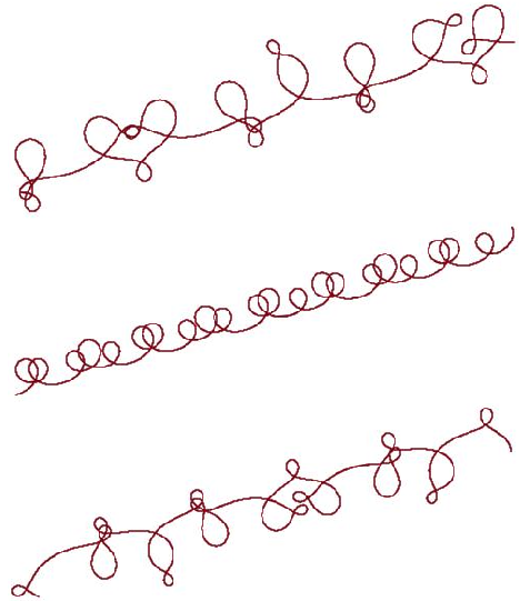
Before making any hypotheses about the geometry of the paths of x,y1,y2x,y_{1},y_{2}, we looked at some plots of these paths – see Figure 7.
Refer to caption
Figure 7: From top to bottom: the trajectories of points x,y1x,y_{1}, and y2y_{2}.

It is immediately obvious that none of the three paths are elastica. However, given the results of the last section, it is plausible that these curves are 2-soliton curves. In this section, we prove that this is the case.

Theorem 7.

If ℓ1≠ℓ2\ell_{1}\neq\ell_{2}, all three planar projections of a tricycling geodesic are 2-solitons.

Proof.

We begin with the xx-curve. We know that its curvature is given by

κx=η2​(t)ℓ22+η1​(t)ℓ12,\kappa_{x}=\frac{\eta_{2}\!\left(t\right)}{\mathit{\ell_{2}}^{2}}+\frac{\eta_{1}\!\left(t\right)}{\mathit{\ell_{1}}^{2}},

and we wish to show, as in the equal length case, that κx\kappa_{x} satisfies the differential equation

a​κ​(t)+b⁡(−d2d​t2​κ​(t)−κ​(t)32)+5​κ​(t)2​(d2d​t2​κ​(t))2+5​κ​(t)​(dd​t​κ​(t))22\displaystyle a\kappa\!\left(t\right)+b\left(-\frac{d^{2}}{dt^{2}}\kappa\!\left(t\right)-\frac{\kappa\!\left(t\right)^{3}}{2}\right)+\frac{5\kappa\!\left(t\right)^{2}\left(\frac{d^{2}}{dt^{2}}\kappa\!\left(t\right)\right)}{2}+\frac{5\kappa\!\left(t\right)\left(\frac{d}{dt}\kappa\!\left(t\right)\right)^{2}}{2} (15)
+3​κ​(t)58+d4d​t4​κ​(t)=0\displaystyle+\frac{3\kappa\!\left(t\right)^{5}}{8}+\frac{d^{4}}{dt^{4}}\kappa\!\left(t\right)=0

for appropriate a,ba,b.

As before, we can set κ0=κx,κ1=κ0′,…​κ4=κ3′\kappa_{0}=\kappa_{x},\kappa_{1}=\kappa_{0}^{\prime},\dots\kappa_{4}=\kappa_{3}^{\prime}, again simplifying the expressions at each step using (11) and algebraic reduction, then replacing the derivatives of κ\kappa by the appropriate κi\kappa_{i}. However, this will simply give us one condition on the two unknowns a,ba,b.

We remedy this situation by differentiating 15 to obtain a fifth order equation for κx\kappa_{x}, requiring an additional computation of κ5=κ4′\kappa_{5}=\kappa_{4}^{\prime}. After algebraic reduction, one obtains the polynomial representation for bb:

b​p​o​l​y\displaystyle bpoly =𝐜​α1​p2​η1ℓ1​ℓ22+𝐜​α2​η2​p2ℓ12​ℓ2−η2​p1​𝐬​α2ℓ12​ℓ2+p122​ℓ22+p222​ℓ22\displaystyle=\frac{\mathit{\,{\bf c}\alpha_{1}\,}p_{2}\eta_{1}}{\ell_{1}\ell_{2}^{2}}+\frac{\mathit{\,{\bf c}\alpha_{2}\,}\eta_{2}p_{2}}{\ell_{1}^{2}\ell_{2}}-\frac{\eta_{2}p_{1}\mathit{\,{\bf s}\alpha_{2}\,}}{\ell_{1}^{2}\ell_{2}}+\frac{p_{1}^{2}}{2\ell_{2}^{2}}+\frac{p_{2}^{2}}{2\ell_{2}^{2}}
−p1​𝐬​α1​η1ℓ1​ℓ22+p122​ℓ12+p222​ℓ12+η222​ℓ12​ℓ22+η1​η2ℓ12​ℓ22+12​ℓ22+12​ℓ12+η122​ℓ12​ℓ22\displaystyle-\frac{p_{1}\mathit{\,{\bf s}\alpha_{1}\,}\eta_{1}}{\ell_{1}\ell_{2}^{2}}+\frac{p_{1}^{2}}{2\ell_{1}^{2}}+\frac{p_{2}^{2}}{2\ell_{1}^{2}}+\frac{\eta_{2}^{2}}{2\ell_{1}^{2}\ell_{2}^{2}}+\frac{\eta_{1}\eta_{2}}{\ell_{1}^{2}\ell_{2}^{2}}+\frac{1}{2\ell_{2}^{2}}+\frac{1}{2\ell_{1}^{2}}+\frac{\eta_{1}^{2}}{2\ell_{1}^{2}\ell_{2}^{2}}

and a considerably longer expression for aa. One can check directly that a,ba,b are constants of motion.

In anticipation of our discussion of the complete integrability of (11), we note that H,p1,p2H,p_{1},p_{2} are constants of motion. Our configuration space is four-dimensional, so we could anticipate an addtional constant of motion, but here we discover two of them, bb and aa. We hypothesize that aa is functionally dependent on bb.

Thus, we augment our polynomial basis P​B2=P​B​⋃{b​p​o​l​y−λ}PB_{2}=PB\,\bigcup\,\{bpoly-\lambda\}, corresponding to a larger ideal I2I_{2}, and use the appropriate tool to compute a new Gröbner basis G​P​B2GPB_{2} for I2I_{2}. One obtains

a​p​o​l​y=p122​ℓ12​ℓ22+p222​ℓ12​ℓ22−λ22+λℓ22+λℓ12−12​ℓ24−12​ℓ12​ℓ22−12​ℓ14modI2.apoly=\frac{p_{1}^{2}}{2\ell_{1}^{2}\ell_{2}^{2}}+\frac{p_{2}^{2}}{2\ell_{1}^{2}\ell_{2}^{2}}-\frac{\lambda^{2}}{2}+\frac{\lambda}{\ell_{2}^{2}}+\frac{\lambda}{\ell_{1}^{2}}-\frac{1}{2\ell_{2}^{4}}-\frac{1}{2\ell_{1}^{2}\ell_{2}^{2}}-\frac{1}{2\ell_{1}^{4}}\mod I_{2}.

Hence, by replacing λ\lambda with bb in the previous formula, we see that aa is in fact a quadratic function of bb.

One can also check, using the same sort of computations, that κy1,κy2\kappa_{y_{1}},\kappa_{y_{2}} both satisfy 15 with the same values of aa and bb just computed. ∎

In the discussion of complete integrability which follows, it will be convenient to use an alternative notation G~=b\tilde{G}=b.

11 Complete integrability of the 2-linkage geodesic equations

In this section we show that the geodesic equations of the 2-linkage (4) are completely integrable. We begin with the case of equal lengths.

Consider the cotangent bundle T∗​𝒞T^{*}{\mathcal{C}} with its standard symplectic form

d​x1∧d​p1+d​x2∧d​p2+d​α1∧d​η1+d​α2∧d​η2.dx_{1}\wedge dp_{1}+dx_{2}\wedge dp_{2}+d\alpha_{1}\wedge d\eta_{1}+d\alpha_{2}\wedge d\eta_{2}.

We have four integrals of motion

H=12[(p1−η1sinα1−η2sinα2)2+(p2+η1cosα1+η2cosα2)2],p1,p2,\displaystyle H=\frac{1}{2}[(p_{1}-\eta_{1}\sin\alpha_{1}-\eta_{2}\sin\alpha_{2})^{2}+(p_{2}+\eta_{1}\cos\alpha_{1}+\eta_{2}\cos\alpha_{2})^{2}],p_{1},p_{2}, (16)
G=κ¨κ+12κ2=p1(p1−η1sinα1−η2sinα2)+p2(p2+η1cosα1+η2cosα2)\displaystyle G=\frac{\ddot{\kappa}}{\kappa}+\frac{1}{2}\kappa^{2}=p_{1}(p_{1}-\eta_{1}\sin\alpha_{1}-\eta_{2}\sin\alpha_{2})+p_{2}(p_{2}+\eta_{1}\cos\alpha_{1}+\eta_{2}\cos\alpha_{2})
+12​(η1+η2)2,\displaystyle+\frac{1}{2}(\eta_{1}+\eta_{2})^{2},

where we used (5) and (7).

Proposition 11.1.

These integrals Poisson commute and they are almost everywhere functionally independent.

Proof.

It is obvious that p1p_{1} and p2p_{2} are in involution with everything. That {H,G}=0\{H,G\}=0 follows from the fact that GG is constant along the trajectories of the Hamiltonian field with the Hamiltonian function HH.

For the second statement, let

u1=η1cosα1+η2cosα2,u2=η1sinα1+η2sinα2.u_{1}=\eta_{1}\cos\alpha_{1}+\eta_{2}\cos\alpha_{2},\ u_{2}=\eta_{1}\sin\alpha_{1}+\eta_{2}\sin\alpha_{2}.

The change of variables

(α1,α2,η1,η2)↦(u1,u2,η1,η2)(\alpha_{1},\alpha_{2},\eta_{1},\eta_{2})\mapsto(u_{1},u_{2},\eta_{1},\eta_{2})

has the Jacobian η1​η2​sin⁡(α2−α1)\eta_{1}\eta_{2}\sin(\alpha_{2}-\alpha_{1}). Assume that this Jacobian doesn’t vanish. Then

H=(p1−v)2+(p2+u)22,G=p12+p22+p2​u1−p1​u2+(η1+η2)22.H=\frac{(p_{1}-v)^{2}+(p_{2}+u)^{2}}{2},\ G=p_{1}^{2}+p_{2}^{2}+p_{2}u_{1}-p_{1}u_{2}+\frac{(\eta_{1}+\eta_{2})^{2}}{2}.

Since p1p_{1} and p2p_{2} are integrals, we need to see when ∇H\nabla H and ∇G\nabla G (as functions of u1,u2,η1,η2u_{1},u_{2},\eta_{1},\eta_{2}) are linearly dependent. The relevant 2×42\times 4 matrix is

(p2+u1−p1+u200p2−p1η1+η2η1+η2).\begin{pmatrix}p_{2}+u_{1}&-p_{1}+u_{2}&0&0\\ p_{2}&-p_{1}&\eta_{1}+\eta_{2}&\eta_{1}+\eta_{2}\\ \end{pmatrix}.

If κ=η1+η2≠0\kappa=\eta_{1}+\eta_{2}\neq 0, then this matrix does not have full rank if and only if u2=p1,u1=−p2u_{2}=p_{1},u_{1}=-p_{2}, but this is impossible because then one would have H=0H=0.

If κ=0\kappa=0, then the matrix does not have full rank if and only if p1​u1+p2​u2=0p_{1}u_{1}+p_{2}u_{2}=0, that is,

p1(η1cosα1+η2cosα2)+p2(η1sinα1+η2sinα2)=0.p_{1}(\eta_{1}\cos\alpha_{1}+\eta_{2}\cos\alpha_{2})+p_{2}(\eta_{1}\sin\alpha_{1}+\eta_{2}\sin\alpha_{2})=0.

This is a hypersurface in the phase space.

To see the meaning of this condition, substitute η1\eta_{1} and η2\eta_{2} from (6) to arrive (as always, applying trigonometric identities) at p2​cos⁡γ−p1​sin⁡γ=0p_{2}\cos\gamma-p_{1}\sin\gamma=0 or, in view of (8), κ˙=0\dot{\kappa}=0. ∎

We briefly discuss the case of unequal lengths. Here, we introduce a slightly different change of variables (which fails to work in the equal length case).

Define

λ1\displaystyle\lambda_{1} =cos⁡(α1)​η1ℓ1+cos⁡(α2)​η2ℓ2,λ2=sin⁡(α1)​η1ℓ1+sin⁡(α2)​η2ℓ2,\displaystyle=\frac{\cos\!\left(\alpha_{1}\right)\eta_{1}}{\mathit{\ell}_{1}}+\frac{\cos\!\left(\alpha_{2}\right)\eta_{2}}{\mathit{\ell}_{2}},\ \lambda_{2}=\frac{\sin\!\left(\alpha_{1}\right)\eta_{1}}{\mathit{\ell}_{1}}+\frac{\sin\!\left(\alpha_{2}\right)\eta_{2}}{\mathit{\ell}_{2}},
μ1\displaystyle\mu_{1} =η2​sin⁡(α2)ℓ1+sin⁡(α1)​η1ℓ2,μ2=η2+η1.\displaystyle=\frac{\eta_{2}\sin\!\left(\alpha_{2}\right)}{\mathit{\ell}_{1}}+\frac{\sin\!\left(\alpha_{1}\right)\eta_{1}}{\mathit{\ell}_{2}},\ \mu_{2}=\eta_{2}+\eta_{1}.

One can check that the determinant of the Jacobian of the transformation (α1,α2,η1,η2)→(λ1,λ2,μ1,μ2)(\alpha_{1},\alpha_{2},\eta_{1},\eta_{2})\rightarrow(\lambda_{1},\lambda_{2},\mu_{1},\mu_{2}) is

η1​η2​(cos⁡(α1)​ℓ1−cos⁡(α2)​ℓ2)​(ℓ12−ℓ22)ℓ13​ℓ23.\frac{\eta_{1}\eta_{2}\left(\cos\!\left(\alpha_{1}\right)\mathit{\ell}_{1}-\cos\!\left(\alpha_{2}\right)\mathit{\ell}_{2}\right)\left(\mathit{\ell}_{1}^{2}-\mathit{\ell}_{2}^{2}\right)}{\mathit{\ell}_{1}^{3}\mathit{\ell}_{2}^{3}}.

We can express our two Hamiltonians HH and G~\tilde{G} in terms of these new variables (WLOG, we henceforth make the assumption that p2=0p_{2}=0):

H=12​λ12−λ1​p1+12​λ22+12​p12,G~=p122​ℓ22−μ1​p1ℓ2​ℓ1+p122​ℓ12+12​ℓ22+12​ℓ12+μ222​ℓ22​ℓ12.H=\frac{1}{2}\lambda_{1}^{2}-\lambda_{1}p_{1}+\frac{1}{2}\lambda_{2}^{2}+\frac{1}{2}p_{1}^{2},\quad\tilde{G}=\frac{p_{1}^{2}}{2\mathit{\ell}_{2}^{2}}-\frac{\mu_{1}p_{1}}{\mathit{\ell}_{2}\mathit{\ell}_{1}}+\frac{p_{1}^{2}}{2\mathit{\ell}_{1}^{2}}+\frac{1}{2\mathit{\ell}_{2}^{2}}+\frac{1}{2\mathit{\ell}_{1}^{2}}+\frac{\mu_{2}^{2}}{2\mathit{\ell}_{2}^{2}\mathit{\ell}_{1}^{2}}.

To prove independence of the two functions HH and G~\tilde{G}, we need to show that the matrix [∇H,∇G][\nabla H,\nabla G] has full rank; but this matrix is easily computed to be:

[λ1−p1λ20000−p1ℓ2​ℓ1μ2ℓ22​ℓ12].\left[\begin{array}[]{cccc}\lambda_{1}-\mathit{p_{1}}&\lambda_{2}&0&0\\ 0&0&-\frac{\mathit{p_{1}}}{\mathit{\ell_{2}}\mathit{\ell_{1}}}&\frac{\mu_{2}}{\mathit{\ell_{2}}^{2}\mathit{\ell_{1}}^{2}}\end{array}\right].

Ignoring the trivial case p1=0p_{1}=0 (where the xx-path is a circle), we see that we have dependence only if both λ2\lambda_{2} and λ1−p1\lambda_{1}-p_{1} are simultaneously equal to zero.

12 Geometric interpretation of the constants of motion G,G~G,\tilde{G}. The planar filament equation

Recall that for the equal length case, we have a constant of motion GG, whereas we had a constant of motion G~\tilde{G} in the unequal case. One can check that if ℓ1=ℓ2=ℓ\ell_{1}=\ell_{2}=\ell, then G~−G=1ℓ2\tilde{G}-G=\frac{1}{\ell^{2}}. In this section we discuss a geometric interpretation of G,G~G,\tilde{G} in their respective cases.

First, assume that ℓ1=ℓ2=1\ell_{1}=\ell_{2}=1.

Fix a point of Q∈T∗​𝒞Q\in T^{*}{\mathcal{C}}, and consider the flow lines of the commuting Hamiltonian vector fields XHX_{H} and XGX_{G} through point QQ, where HH and GG are as in (16).

Project these curves to the plane. The first curve is the trajectory x⁡(t)x(t), an elastica. Let (T⁡(t),N⁡(t))(T(t),N(t)) be the Frenet frame along this curve. The tangent vectors to the second curve provide a vector field ξ\xi along this elastica. This vector field can be written as ξ=u​T+v​N\xi=uT+vN, where uu and vv are functions of tt.

Theorem 8.

One has

u⁡(t)=1+g−12​κ2​(t),v⁡(t)=−κ˙​(t),u(t)=1+g-\frac{1}{2}\kappa^{2}(t),\ v(t)=-\dot{\kappa}(t),

where κ⁡(t)\kappa(t) is the curvature of the curve x⁡(t)x(t), and gg is the value of the integral GG at point QQ.

Proof.

The projection of the vector XG~​(Q)X_{\tilde{G}}(Q) on the plane is the vector

ξ=(Gp1,Gp2)\displaystyle\xi=(G_{p_{1}},G_{p_{2}}) =(2p1−η1sinα1−η2sinα2,2p2+η1cosα1+η2cosα2)\displaystyle=(2p_{1}-\eta_{1}\sin\alpha_{1}-\eta_{2}\sin\alpha_{2},2p_{2}+\eta_{1}\cos\alpha_{1}+\eta_{2}\cos\alpha_{2})
=(p1+cos⁡γ,p2+sin⁡γ),\displaystyle=(p_{1}+\cos\gamma,p_{2}+\sin\gamma),

where the last equality is due to (3). One has

T=(cos⁡γ,sin⁡γ),N=(sin⁡γ,cos⁡γ),T=(\cos\gamma,\sin\gamma),N=(\sin\gamma,\cos\gamma),

and the linear equation ξ=u​T+v​N\xi=uT+vN has the solution

u=1+p1​cos⁡γ+p2​sin⁡γ,v=−p1​sin⁡γ+p2​cos⁡γ.u=1+p_{1}\cos\gamma+p_{2}\sin\gamma,v=-p_{1}\sin\gamma+p_{2}\cos\gamma.

Use equations (7) and (8) and the definition of GG to conclude:

u=1+κ¨κ=1+g−12​κ2​(t),v⁡(t)=−κ˙​(t),u=1+\frac{\ddot{\kappa}}{\kappa}=1+g-\frac{1}{2}\kappa^{2}(t),\ v(t)=-\dot{\kappa}(t),

as claimed. ∎

Thus the vector field ξ\xi is a linear combination of the unit tangent field TT and the planar filament vector field 12​κ2​T+κ˙​N\frac{1}{2}\kappa^{2}T+\dot{\kappa}N, see [6]. Note that the flow of this field takes the elastic curves to elastic curves, in agreement with the fact that the flows of the Hamiltonians HH and GG commute.

If ℓ1≠ℓ2\ell_{1}\neq\ell_{2}, we have the analogous statement, proved by the computer algebra techniques already discussed.

Theorem 9.

One has

u⁡(t)=g~−12​κ2​(t),v⁡(t)=−κ˙​(t),u(t)=\tilde{g}-\frac{1}{2}\kappa^{2}(t),\ v(t)=-\dot{\kappa}(t),

where κ⁡(t)\kappa(t) is the curvature of the curve x⁡(t)x(t), and g~\tilde{g} is the value of the integral G~\tilde{G} at point QQ.

13 Concluding remarks

Inspired by papers [1, 2], we have obtained a 2-linkage model which exhibits the fundamental observation in those references: the vertices of the moving linkage sweep out curves of interesting geometry. Amusingly, our problem, involving a completely non-integrable distribution, is completely integrable.

It is clear that there is much more worth studying related to this problem. Here are some open questions:

  • •

    Elastic curves have been studied in the context of spherical and hyperbolic geometry, see [8]; additionally, analogues of the planar filament flow exist in those geometries as well, see [7]. This suggests that our 2-linkage problem could be amenable to study is these contexts too.

  • •

    In this paper, we have by no means solved the geodesic equations, we have only shown a certain striking property of the projection of the solutions to the plane. Can these equations be solved exactly?

  • •

    Paper [2] extends the work in [1] to 1-linkages in ℝn{\mathbb{R}}^{n}. We expect the results of our paper to be extendable to higher dimensional cases as well.

  • •

    Isospectrality is a nearly universal property of integrable systems, although this can take some work to uncover. To give one example, the problem of integrability of geodesics on the ellipsoid goes back to Jacobi, but the isospectral framework for the problem was discovered by Moser [12]. Does such a framework appear in the case of our problem?

  • •

    The starting point of our work was a different sub-Riemmanian problem, concerning the geodesic motion of a 2-linkage x​y​zxyz subject to the following non-holonomic constraint: the velocity of point yy is aligned with the segment x​yxy, and the velocity of the point zz with the segment z​yzy, see Figure 8. The lengths of the two segments are fixed, and the length a horizontal curve is defined as the length of its xx-projection to the plane.

    Figure 8: Another 2-linkage.

    Rather than modeling bicycle, this is a model of tractor trailer, which is a well studied topic; see, e.g., [18] and the references therein. Unfortunately, we did not obtain meaningful results in this case, but we think that it merits a study. See Figure 9 for an example of the planar projections of a geodesic.

    Refer to caption
    Refer to caption
    Refer to caption
    Figure 9: The x,yx,y, and zz projections of a geodesic.
  • •

    Why stop at 2-linkages? There are obvious nn-linkage problems to consider, where the non-holonomic constraints apply to the midpoints of each segment, and one wants to extremize the length of the trajectory of either vertex (they have the same length).

    In the case of three or more segments, the topology of the linkage is not unique. In the case of 3-linkages, one can have a “linear” linkage, or a “spokewheel” linkage, see Figure 10.

    Figure 10: Two topologically different 3-linkages.

    Our last figures give examples of the trajectories in the “linear” and “spokewheel” cases. Perhaps one or both of these problems is integrable, as well extensions to linkages with four or more links. See Figure 11, 12.

Refer to caption
Figure 11: The trajectories of four vertices of a “linear” 3-linkage, the case of three unequal lengths.
Refer to caption
Figure 12: The trajectories of four vertices of a “spokewheel” 3-linkage, the case of three unequal lengths. The first trajectory is of that of the middle point.

References

  • [1] A. Ardentov, G. Bor, E. Le Donne, R. Montgomery, Yu. Sachkov. Bicycle paths, elasticae and sub-Riemannian geometry. Nonlinearity 34 (2021), 4661–4683.
  • [2] G.  Bor, C.  Jackman, S.  Tabachnikov. Bicycling geodesics are Kirchhoff rods. Nonlinearity 36 (2023), 3572–3602.
  • [3] G. Bor, M. Levi, R. Perline, S. Tabachnikov. Tire track geometry and integrable curve evolution. Int. Math. Res. Notices, 2020, no. 9, 2698–2768.
  • [4] E. Coddington, N. Levinson. Theory of ordinary differential equations. McGraw-Hill, New York-Toronto-London, 1955.
  • [5] R. Foote, M. Levi, S. Tabachnikov. Tractrices, bicycle tire tracks, hatchet planimeters, and a 100-year-old conjecture. Amer. Math. Monthly 120 (2013), 199–216.
  • [6] J. Langer, R. Perline. The planar filament equation. Mechanics day (Waterloo, ON, 1992), 171–180. Fields Inst. Commun., 7. Amer. Math. Society, Providence, RI, 1996.
  • [7] Langer, J., and Perline, R. Local geometric invariants of integrable evolution equations. J. Math. Phys.35(1994), 1732–1737.
  • [8] Langer, J., and Singer, D.A. (1984). The total squared curvature of closed curves. Journal of Differential Geometry 20 (1984) 1–22.
  • [9] D. Lazard. Gröbner bases, Gaussian elimination and resolution of systems of algebraic equations. Computer algebra (London, 1983), 146–156, Lecture Notes in Comput. Sci., 162, Springer, Berlin, 1983.
  • [10] R. Montgomery. A Tour of SubRiemannian Geometry. Amer. Math. Soc., Providence, RI (2006).
  • [11] R. Montgomery. A survey of singular curves in sub-Riemannian geometry. J. Dynam. Control Systems 1 (1995), 49–90.
  • [12] J. Moser. Various Aspects of Integrable Hamiltonian Systems. Dynamical systems (C.I.M.E. Summer School, Bressanone, 1978), pp. 233–289, Birkhäuser, Boston, Mass., 1980.
  • [13] R. Perline. The role of elastica in geometry, Nonlinearity and Geometry, Warsaw, 1995.
  • [14] C. Rogers, W. Schief. Bäcklund and Darboux Transformations. Cambridge Univ. Press, Cambridge, 2002.
  • [15] D. Singer. Lectures on elastic curves and rods. Curvature and variational modeling in physics and biophysics, 3–32, AIP Conf. Proc., 1002, Amer. Inst. Phys., Melville, NY, 2008.
  • [16] B. Sturmfels What is … a Gröbner basis? AMS Notices 52 (2005), 1199–1200.
  • [17] S. Tabachnikov. On the bicycle transformation and the filament equation: Results and conjectures. J. Geom. Phys. 115 (2017), 116–123.
  • [18] D. Tilbury, R. Murray, S. Sastry. Trajectory generation for the n-trailer problem using Goursat normal form. IEEE Trans. Automat. Control 40 (1995), 802–819.