Continuous Time Evidential Distributions for Irregular Time Series
Abstract
Prevalent in many real-world settings such as healthcare, irregular time series are challenging to formulate predictions from. It is difficult to infer the value of a feature at any given time when observations are sporadic, as it could take on a range of values depending on when it was last observed. To characterize this uncertainty we present EDICT, a strategy that learns an evidential distribution over irregular time series in continuous time. This distribution enables well-calibrated and flexible inference of partially observed features at any time of interest, while expanding uncertainty temporally for sparse, irregular observations. We demonstrate that EDICT attains competitive performance on challenging time series classification tasks and enabling uncertainty-guided inference when encountering noisy data. Code is available at https://github.com/twkillian/EDICT.
Keywords:
Evidential Deep Learning, Irregular Time Series, Uncertainty Quantification, Continuous Time Models, Healthcare1 Introduction
Irregularly-sampled, multivariate time series data are common across many real-world applications, including healthcare (Jensen et al. 2014), meteorology (Shi et al. 2015), and business (Batres-Estrada 2015). These data are characterized by missing and/or irregular observations, inducing inherent uncertainty about the value of unobserved features. Traditional machine learning (ML) approaches manage this irregularity through imputation and resampling of the data to impose full observations recorded at evenly spaced time steps. However, the choice of resampling rate and how to fill missing intervals can introduce unnecessary bias in the data used to train models, limiting their reliability. To build reliable predictive models from irregular data it is crucial to model the distribution of the time series—conditioned on sparse previous observations—to infer possible values of unobserved features and allow the natural presentation of the data to dictate what the model learns. Additionally, precise uncertainty estimates can help interpret predictive confidence and assess the robustness of model predictions.
Prior approaches that attempt to quantify uncertainty over irregular time series either stabilize a learned latent representation of the data (De Brouwer et al. 2019; Fortuin et al. 2020) or forecast future values (Stankeviciute et al. 2021; De Brouwer et al. 2022; Sun and Yu 2022) as a means to identify possible outcomes of the current observed state. However, these approaches either do not connect the estimated representations with the reliability of downstream predictions (De Brouwer et al. 2019; Sun and Yu 2022), or fail to provide continuous-time projections of missing values in the time series (Fortuin et al. 2020; Stankeviciute et al. 2021).
Rather than relying on indirect estimates of the predictive distribution (Gal and Ghahramani 2016b), efforts with a recently introduced approach called evidential learning aim to model the variance in predictive distributions directly, formulated as an evidence acquisition process (Sensoy et al. 2018; Malinin and Gales 2018; Amini et al. 2020; Charpentier et al. 2020). These methods provide scalable and calibrated uncertainty estimates but have only been developed for static, univariate supervised classification (Sensoy et al. 2018) and regression (Amini et al. 2020; Meinert and Lavin 2021) problems. The extension of these techniques to irregularly sampled time series presents nuanced complexities due to the sporadic observations, high rates of missingness, and data generation occurring through a dynamic, continuous-time process.
In this work, we present a method to process multivariate irregular time series by through a neural ODE (Kidger 2021) to construct a latent representation that is used to predict the parameters of a higher-order probability distribution (Figure 1). Under this paradigm, the training data is assumed to provide evidence for the predicted distribution and estimated uncertainties are associated with erroneous model behavior or out of distribution input data. This evidential distribution provides calibrated, temporally correlated uncertainty estimates over the multivariate time series and enables robust, uncertainty-guided classification using the learned latent representation. In total, this work makes the following contributions:
- 1)
Formulation of an evidential learning approach for sequential, continuous-time problems;
- 2)
A scalable method for inferring Evidential Distributions in Continuous Time (EDICT), deriving uncertainty estimates without the need for sampling during inference, Monte Carlo estimation, or training on out-of-distribution data;
- 3)
Evaluation of the inferred evidential distribution on both interpolation and extrapolation settings for irregular time series, demonstrating superior accuracy and calibration;
- 4)
Demonstration of uncertainty-guided inference in classification settings, correcting for noisy observations to stabilize predictions and improve performance.
2 Uncertainty Estimation with Evidential Learning
Calibrated estimates of neural network (NN) uncertainty are important for understanding how well the model will perform on unseen data, derive measures of confidence, as well as providing feedback on data missingness and irregularity. Bayesian methods have been used to characterize model (e.g., epistemic) uncertainty by placing probabilistic priors on NN parameters, using variational approximations and Monte-Carlo sampling to estimate output variance (Kendall and Gal 2017). However, contemporary NNs are often too large and complex for these methods to be feasible, with additional challenges in choosing the right approximation and priors on the parameters (Yao et al. 2019).
Rather than placing priors on network weights as with Bayesian NNs, recent approaches place priors directly over a Gaussian likelihood function of the network’s predictions by framing model learning as an evidence acquisition process (Sensoy et al. 2018; Malinin and Gales 2018; Amini et al. 2020; Meinert and Lavin 2021), motivated by Dempster-Shafer theory (Shafer 1976). In these approaches, the NN produces the hyperparameters of the posterior distribution via maximum likelihood estimation (Charpentier et al. 2020), where the support of the distribution is derived directly from the training data. Thus, evidential learning provides a scalable, well-calibrated uncertainty estimation technique by eliminating the need for sampling-based or variational approaches.
In this paper, we present a multivariate formulation of evidential distributions for continuous-time NN models, termed Evidential Distributions in Continuous Time (EDICT). EDICT enables prediction of feature evolution as well as calibrated model uncertainties over sequential observations made at irregular time intervals. To our knowledge, EDICT is the first method to develop evidential distributions with corresponding measures of uncertainty over high-dimensional features sets as well as in sequential settings.
3 Evidential Distributions in Continuous Time
In this section we formalize our problem statement and outline the EDICT method, specifically focused on developing estimates of NN uncertainty for irregular time series. This is done without the need for sampling during inference (Fortuin et al. 2020; Kingma et al. 2015), Monte Carlo estimation (Gal and Ghahramani 2016b; Gal and Ghahramani 2016a), or training on out-of-distribution data (Hafner et al. 2020; Malinin and Gales 2018; Malinin et al. 2020) which facilitates far more scalable uncertainty quantification.
3.1 Problem setup
We consider a -dimensional irregular time series with finite observation horizon and infer a distribution over the feature space, conditioned on previous observations, to forecast the possible values of any feature before it is observed again. We assume that each time series is measured at time points that may arise sporadically, with some subset of the features present at each observation. Additionally, we assume that a representation of the latent generating process of the observable time series can be inferred in continuous time. After time has been reached, and the allowed observation window has closed, we expect to formulate a prediction about some target characteristic of the time series.
For convenience in modeling, we assume that is drawn from a multivariate Normal distribution with mean and covariance such that 11 1 Time dependence of the parameters of the generating distribution is assumed through the remainder of this paper unless necessary to establish context.. We aim to model these unknown functions by predicting hyperparameters of their generating distribution using the learned continuous-time representation formed from prior observations of . Specifically, we place priors on and to flexibly account for the possible variance among features of the observed time series , developing an evidential distribution in continuous time. Next we describe:
- i)
How is updated in continuous time with neural ODEs;
- ii)
How the evidential learning objective is used to formulate continuous-time distributions;
- iii)
How the resulting Evidential Distribution in Continuous Time (EDICT) can be used to guide the reweighting of noisy and out-of-distribution observations;
- iv)
How inferred from EDICT can then be used to train downstream classification models to predict underlying characteristics or target values of the time series .
3.2 Continuous-time Representations of Irregular Time Series
Our evidential learning objective maximizes the likelihood of observing , given the parameters of the generating distribution and the prior observations :
We resolve conditional dependence on by encoding the observations in a continuous-time, recurrent latent representation . Continuous-time (CT) models for sequential processing of information were originally proposed as an extension of recurrent NNs (Funahashi and Nakamura 1993; Chow et al. 2000). Recently, deep learning models utilizing differential equation solvers have extended these ideas (Chen et al. 2018; Rubanova et al. 2019; Kidger 2021), enabling a flexible basis for learning the latent dynamics of temporal observations, including those that are irregularly sampled. CT models form a latent representation of the dynamics underlying the data generating process that is propagated between recorded observations.
To update once an observation has been made, we employ a GRU-inspired procedure (De Brouwer et al. 2019) that (1) propagates between observations using a neural ODE , and (2) adjusts with an approximate Bayesian mechanism, , once an observation is made. Both of these mechanisms are represented as NNs. To produce the parameters of the generating distribution a third NN, is used to map to . If needed, an additional function may be used to process the set of observed features to improve the update to . Together, the process of propagating and updating the representation given observations is as follows:
- 1.
Propagate over the interval between observations:
- 2.
Update once an observation is made:
- 3.
Produce to infer the distribution over via: ,
where and denote the time directly before and after . We use this procedure to create a CT representation of the irregular time series. The resulting representation is then used to produce the hyperparameters of an evidential distribution, as outlined in the next subsection.
3.3 Constructing EDICT
Estimating parameters of the evidential distribution
We assume the time series is drawn from a multivariate Normal distribution with mean and covariance : . We formulate the evidential distribution by placing priors on the parameters and using a conjugate prior, the Normal Inverse Wishart (NIW) distribution. This entails placing a Gaussian prior on and an Inverse-Wishart prior on :
The parameters of this evidential conjugate prior can be interpreted in terms of “virtual observations” (Jordan 2009) in support of the evidence collected via the training data. In our evidential learning framework, the parameters are produced by a learned function of the CT representation . Thus, any set of features included with the next observation will improve the posterior estimates of the evidential distribution. The parameters of the evidential distribution are inferred and updated through time to approximate the full time series .
Within this evidential framework, the objective is to maximize the likelihood of observing given and prior observations . We formulate this using the evidential NIW prior as:
| (1) | ||||
where denotes the multivariate, -dimensional -distribution (Meinert and Lavin 2021)22 2 See Appendix C.2 and C.3 of Meinert and Lavin 2021. By predicting the parameters using the prior observations to encode and propagate , we directly estimate the likelihood without the need for sampling or other complex inference techniques.
Using inferred NIW parameters to make predictions
By learning a CT representation (Section 3.2), producing , and learning the NIW evidential distribution, we can flexibly predict the values of at any time before the observation horizon . With predicted parameters of the NIW distribution, predictions and associated measures of uncertainty of missing features can be made directly. These measures of uncertainty include both irreducible stochasticity in the data distribution (i.e., the aleatoric uncertainty) and the accuracy of the model (i.e., the epistemic uncertainty):
The epistemic uncertainty is determined by the variance of the predictions formulated through the NIW. We provide a demonstration of EDICT in Figure 2 using a 2D synthetic dataset of anti-correlated periodic signals with decaying amplitude and random phase shifts. Here, EDICT quickly resolves the correct dynamics of the signals after a small number of observations. EDICT smoothly propagates the predicted uncertainty over intervals where no observations are made, and appropriately contracts this estimate once an observation is made.
Optimizing NIW parameters
All modules that contribute to the formation of EDICT (CT representation learning and prediction of ) are optimized as a multi-task learning problem. First, we seek to maximize the model evidence according to the observations of . We do this by minimizing the negative log-likelihood of the multivariate -distribution (Eqt. 1; ). Second, we want to promote that the inferred NIW distribution covers the empirical distribution of the recorded observations through a Kullback-Leibler constraint (). This forces the model to mimic a Bayesian update (De Brouwer et al. 2019) when observations are made. Finally, the learned evidential distribution is further regularized by reducing the inferred evidence when the prediction is wrong () (Amini et al. 2020). Altogether our total objective for learning the continuous-time evidential distribution is:
| (2) |
where are hyperparameters that modify the effect of the two regularization terms. Details on this objective (Section B) and on EDICT and its training (Section D) are in the Appendix.

3.4 Downstream prediction with EDICT
With a well-calibrated evidential distribution in continuous time, EDICT enables two key abilities in formulating downstream predictions for a target given an input time series .
First, EDICT learns a rich representation of the latent dynamics of the time series, , that is influenced by the inferred evidential distribution and corresponding estimates of uncertainty. Using this representation , we can develop expressive prediction models of the target label . We demonstrate this empirically through classification experiments using various irregular time series datasets (Section 4), with results in Section 5.2.
Second, EDICT learns an underlying distribution that provides an explicit measure of the likelihood of any future observation. Consider a deployment scenario where observed features begin to shift out of distribution or become overly noisy through time, common in persistent sensing settings. When constructing a CT representation, the predicted mean of the distribution “jumps” to cover these noisy observations, resulting in an unstable representation . To address this, we design an algorithm that uses EDICT to infer how reliable an observation is and “correct” it, if needed, using the predicted mean and variance as a form of reweighting. This stabilizes the update of the CT representation and thereby the predicted mean of the distribution. We designate this as Evidential Distribution Guided Reweighting (EDGR) (Algorithm 1). Using EDGR within EDICT allows for practical use of the learned distribution in downstream classification to provide uncertainty-guided predictions.
EDGR establishes whether an observation is noisy enough to require reweighting if it deviates more than from the predicted mean , where is a hyperparameter to balance the stability of EDICT with reductions in the contributions of noisy data. We show the utility of EDGR through experiments with additive heteroskedastic noise of increasing magnitude through time (Section 5.2).
4 Experiments
4.1 Datasets
We evaluate EDICT on one synthetic and four publicly available irregular time series datasets (Table 1):
- 1.
Synthetic: We sparsely sample 3 periodic features, forming a binary prediction task. The outcome is informed by feature 1 or 2 with the third feature being uninformative.
- 2.
Gestures: The uWave dataset (Liu et al. 2009) contains recordings of a three-axis accelerometer used to “draw” 8 pre-defined templates. We subsample the data to keep a random 10% of all observations.
- 3.
Activity: The Human Activity dataset (Kaluža et al. 2010) contains recordings of subjects performing various physical activities, consisting of the 3D position of 4 monitors (12 features in total).
- 4.
PhysioNet: The goal is to predict in-hospital mortality for patients in the ICU. The task is provided by the PhysioNet/Computing in Cardiology Challenge 2012 (Silva et al. 2012).
- 5.
MIMICMort: The task is to predict in-ICU mortality from labs and vitals. We use MIMIC-Extract (Wang et al. 2020), which is derived from the MIMIC-III Clinical Database (Johnson et al. 2016).
| Dataset | # Classes | # Features | # Samples |
|---|---|---|---|
| Synthetic | 2 | 3 | 10,000 |
| Gestures | 8 | 3 | 4,478 |
| Activity | 7 | 12 | 10,486 |
| PhysioNet | 2 | 34 | 7,990 |
| MIMICMort | 2 | 49 | 24,391 |
Dataset details, including preprocessing procedures, are contained in the Section C in the Appendix.
4.2 Baselines
For baseline comparison, we focus on methods that develop measures of uncertainty based on the continuous-time arrival of irregular observations. Our primary baseline is GRU-ODE-Bayes (De Brouwer et al. 2019), which uses a GRU-based ODE to evolve the hidden state continuously between observations, while using a Bayesian update to transform the hidden state at each observation. To our knowledge, GRU-ODE-Bayes is the only method, prior to our present work, that can provide predicted distributions for continuous-time observations in multivariate, irregularly-sampled time series.
To evaluate downstream classification, we also compare against contemporary NN methods that handle irregular time series for classification alone: (i) Interpolation Prediction Network (IPN) (Shukla and Marlin 2019), (ii) GRU-D (Che et al. 2018), (iii) Set Functions for Time Series (SeFT) (Horn et al. 2020). These methods do not produce uncertainty estimates as EDICT does, but are included for completeness.
4.3 Experimental Setup
All datasets are split into training, validation, and evaluation subsets following a 70/10/20 split, stratified such that the proportion of class labels is consistent among all subsets. The same data splits are used when training EDICT and on the downstream classification tasks. Results in Section 5 are derived from the evaluation subset. We perform three types of experiments to evaluate EDICT.
4.3.1 Uncertainty evaluation and calibration
As our primary empirical evaluation, we train EDICT models on each dataset using the loss shown in Equation 2, varying and among other hyperparameters (see Appendix, Section D). Note that this procedure is unsupervised, i.e., it does not make use of exogenously provided task labels but rather utilizes the sequentially gathered feature observations themselves. We evaluate the quality of the predictions made by EDICT and their accompanying uncertainty measures via its evidential distribution, compared against GRU-ODE-Bayes and its inferred distribution. We assess the following metrics (Sun and Yu 2022):
- 1.
Coverage. We want inferred model uncertainties to be well calibrated. For , we select the confidence region of the distribution and compute the fraction of observed data within it. We quantify this measure of coverage with Expected Calibration Error (ECE) (details in Appendix, Section D).
- 2.
Efficiency. It is preferable for a calibrated model to have small area (i.e., the width of the confidence intervals). We plot the average width of the confidence region over all .
- 3.
Forecasting error. We evaluate how far the mean of the predictive distribution is from the actual observation by computing the Mean Squared Error (MSE).
We evaluate these metrics in both interpolation (Section D) and extrapolation (Figure 3, Table 2) settings. We hold out a random 10% of observations prior to time . During training, we only expose the model to the remaining data in . We evaluate interpolation by evaluating with the held-out data. For extrapolation, we use unobserved data from . Each metric is calculated separately for each time series, and a confidence interval over each metric is generated as one standard deviation over the samples in the dataset.
4.3.2 Performance in downstream decision-making
Next, we evaluate EDICT’s performance in downstream classification tasks. We freeze the weights of the EDICT model, and train a downstream linear classifier using the embedded latent representations of . We compute the accuracy of the predictions, and generate confidence intervals by repeating this procedure with three random seeds.
4.3.3 Prediction over noisy observations
To evaluate our method in a realistic scenario where the test samples may be out of distribution from the training data (e.g., due to sensor failure), we experiment with injecting temporally compounding heteroskedastic noise into the test-set observations with the degree of variance being a function of time. For each dataset, a range of 10 noise levels are chosen as the base rate for this exponentially compounding amount of noise (details in the Section D).
We demonstrate the utility of EDICT for uncertainty-guided classification by using EDGR (Section 3.4, Alg. 1) to reweight observations identified as outliers. We compare the performance of this method on AUROC against base EDICT (i.e., no reweighting), as well as against an alternative approach which clips observations based on the data distribution’s population mean. In all experiments, we use , corresponding to a 95% confidence interval.
5 Results
We first evaluate the quality of EDICT’s uncertainty bounds over feature values and show that EDICT achieves better calibration than GRU-ODE-Bayes on several datasets (Section 5.1). EDICT’s performance in downstream classification is then demonstrated to match current state of the art baselines while also providing calibrated uncertainty metrics (Section 5.2). Finally, we illustrate the flexibility of EDICT’s uncertainty intervals in accounting for noisy observations. We show that EDICT with EDGR outperforms the the comparative baselines at high noise levels, particularly in complex, real-world datasets (Section 5.3).
5.1 Evidential Distribution Calibration

In Figure 3 and Table 2, we compare the calibration of the distributions predicted by EDICT and GRU-ODE-Bayes when extrapolating beyond the observed data for the Synthetic and MIMICMort datasets (comparisons for all datasets, including interpolation results, can be found in the Appendix, Section D). We find that EDICT has much lower MSE than GRU-ODE-Bayes on Synthetic and Gestures, and the MSEs are comparable on the remaining three datasets when confidence intervals are taken into account (Table 2). On the Synthetic dataset, EDICT achieves greatly improved efficiency relative to GRU-ODE-Bayes and exhibits strong calibration performance relative to both the ideal and GRU-ODE-Bayes baseline coverage (Figure 3A) in all other datasets. On the real-world MIMICMort dataset, EDICT demonstrates strong coverage, indicating well-calibrated model uncertainties (Figure 3B).
| EDICT | GRU-ODE-Bayes | ||||
|---|---|---|---|---|---|
| Dataset | MSE | ECE | MSE | ECE | |
| Synthetic | |||||
| Gestures | |||||
| Activity | |||||
| PhysioNet | |||||
| MIMICMort | |||||
5.2 Downstream Classification
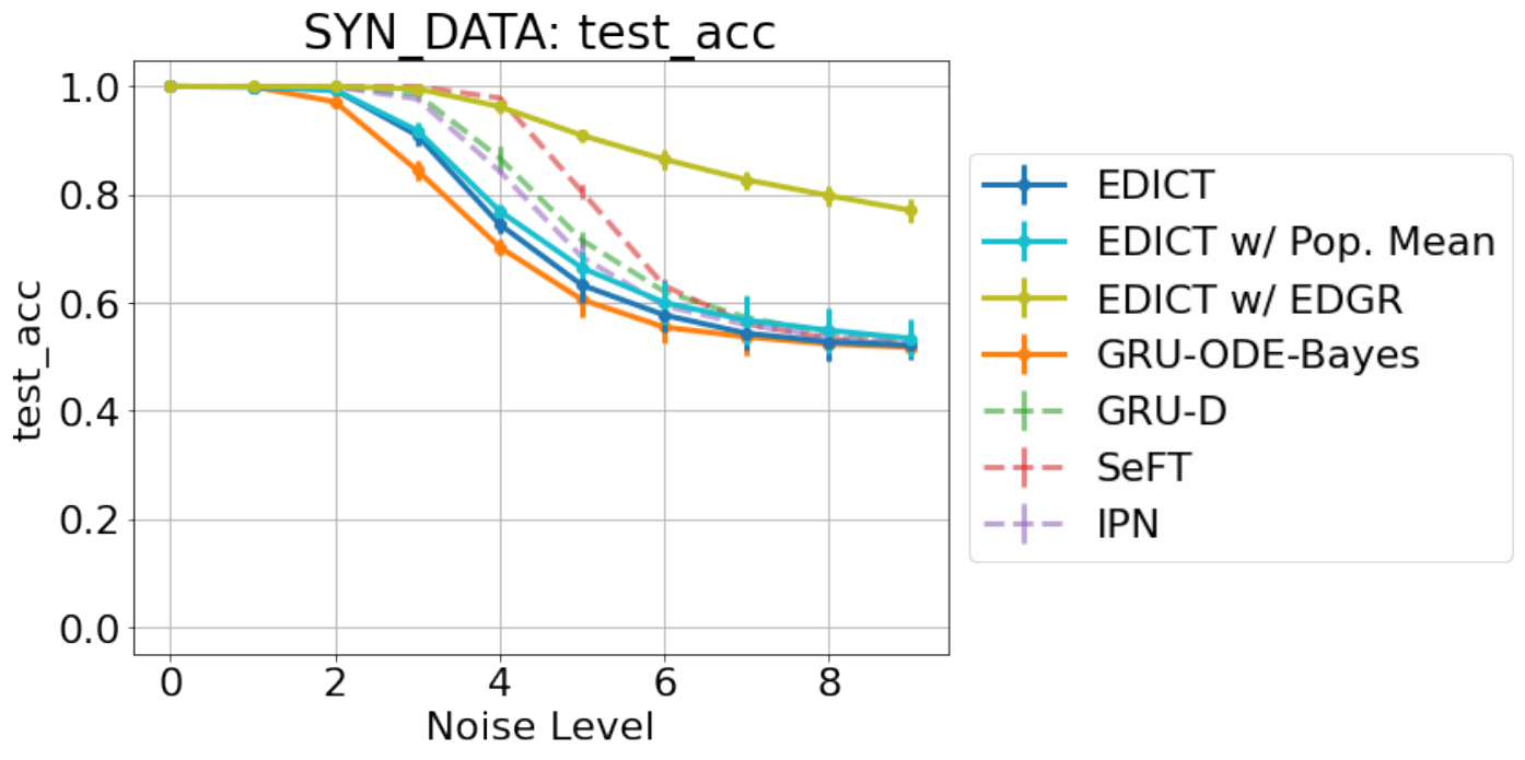
One major goal of learning effective latent representations for irregularly sampled time series is to achieve strong performance on some downstream task. To this end, we compare the test-set AUROC of EDICT with a set of baselines in classifying irregular time series (Figure 4; Appendix, Section D.3). On the zero-noise classification task (train and test samples drawn from the same distribution), EDICT matches the performance of current standard approaches (Figure 4, noise level 0). Critically, the majority of evaluated baselines fail to provide uncertainty intervals over intermediate noise values. Variations of EDICT and GRU-ODE-Bayes are the only methods in Figure 4 that do so, indicating EDICT’s ability to enable both strong downstream decision-making and calibrated uncertainties. In high noise settings, all baselines have reduced performance where prediction quality is near chance. Across all methods tested, EDICT is more resistant to performance decay caused by noisy observations. The performance demonstrated in Figure 4 suggests that the latent learned by EDICT and directly influenced by its evidential distribution – is more robust to these outlying, noisy observations.

5.3 Correcting for Noisy Observations
One main advantage of EDICT over most baselines is the ability to infer a distribution over feature values in continuous time. Here, we demonstrate one utility of this distribution, by using it to clip values identified as outliers in the presence of noisy data not seen during training. To this end, we designed an algorithm, EDGR, that leverages the learned evidential distribution to identify outliers and reweight them according to the uncertainty of the observed feature. In Figure 4 (and Appendix, Section D.3), we find that EDICT with uncertainty-guided reweighting (EDICT w/ EDGR) allows the model to maintain robust performance for high noise levels, especially for Synthetic, Gestures, Physionet, and MIMICMort, where higher noise levels cause all baseline models, including GRU-ODE-Bayes, to fail.
Taking these results together, we observe that EDICT performs best when there are relationships to be inferred among all feature dimensions in continuous time. Of the experiments presented in this work, four of the five datasets have this characteristic, excepting Activity. The features within the Activity time series are slightly disjoint from one another and are not time aligned. Due to this, set-based interpolation methods such as SeFT and IPN are better suited for this dataset. Among all other datasets, we see that embedding the irregular time series in a continuous-time latent representation allows us to adequately account for missing features when predicting the evidential distribution. In these settings EDICT enables robust prediction performance and the ability to leverage the distributional estimates to mitigate OOD observations.
6 Related Work
Learning from irregular time series
Irregular time series contain observations sampled at uneven times from constantly-changing environments, representative of most real-world settings. Such irregularity is challenging for machine learning, especially when multiple variables are observed simultaneously. Many traditional works tackle irregularity through imputation, resampling the values of an irregular series at a set of new, evenly spaced timesteps (Lipton et al. 2016; Zheng et al. 2017; Che et al. 2018; Li and Marlin 2020; Mozer et al. 2017). While imputation has proven useful in forecasting (Cao et al. 2018) and classification (Che et al. 2018), there are serious drawbacks. For instance, choosing a good resampling rate is crucial (Hartvigsen et al. 2023), yet the optimal rate is often unknown a priori. Furthermore, imputation can introduce unnecessary bias, since irregularity is often natural. These limitations have recently spurred major efforts on learning continuous-time models of irregular time series.
Continuous-time models and uncertainty estimation
Continuous-time methods have been shown to learn the latent dynamics of irregular time series (Morrill et al. 2022; Kidger 2021; Rubanova et al. 2019; Jia and Benson 2019; Hasani et al. 2021; Schirmer et al. 2022; Salvi et al. 2022; Hasani et al. 2022). By providing access to representations at any desired time, these models are more flexible than their imputation-based precursors and are now the state-of-the-art approach to many problems. Originally grounded in RNNs (Funahashi and Nakamura 1993; Chow et al. 2000), most recent approaches succeed by parameterizing differential equations with NNs (Kidger 2021; Rubanova et al. 2019; Jia and Benson 2019). Despite recent advances, uncertainty quantification for these continuous-time models remains in its infancy (Graf et al. 2021), although there have been successes estimating the distributions of discrete time series (Rasul et al. 2021a; Rasul et al. 2021b; Yu et al. 2021). Indeed, some works have included uncertainty for multivariate irregular time series, especially through multi-task Gaussian processes (Cheng et al. 2020; Fortuin et al. 2020; Ghassemi et al. 2015). However, these approaches are notoriously difficult to scale to high dimensions and fall prey to the resampling challenges native to imputation methods. Our work directly addresses these needs by quantifying uncertainty for continuous-time models while maintaining scalability as a byproduct of using standard deep learning frameworks to construct our evidential distributions.
7 Discussion
In this paper we introduce Evidential Distributions in Continuous Time (EDICT), a continuous-time formulation of evidential deep learning for sequential and irregular time series problems. EDICT enables temporally correlated estimates of uncertainty over intervals of missing observations and inconsistent measurement patterns, providing stability to latent inference processes of the underlying data. EDICT maintains distributional calibration on a variety of complex datasets, while achieving competitive performance among current state of the art time series classification algorithms. Further, by virtue of the inferred evidential distribution, EDICT enables improved robustness in the presence of noisy observations, avoiding drastic degradation of model performance through uncertainty-guided inference.
In contrast to traditional uncertainty quantification approaches in contemporary deep learning, EDICT forms its distributions without the use of sampling, complex variational approximations, or training on out-of-distribution data. Further, it encodes the observations of an irregular time series without needing to make a priori assumptions about how to best manage intervals of missingness. This directly overcomes the need to construct imputation strategies manually or to discretize the temporal component of the observed data. As such, we propose EDICT as a flexible method for making predictions and inferring calibrated uncertainties from irregular time series.
Limitations and Future Work
The flexibility and scalability of our approach holds promise for potential use in challenging real-world scenarios where forecasting the evolution of features is equally as important as making accurate inference of their current values. Our proposed continuous-time evidential distributions enable both objectives and may provide a decision support framework for practical use by domain experts. While promising, there are some distinct limitations of EDICT. We did not test the method against asymmetric noise models when evaluating the performance of EDGR, the adaptive reweighting approach formulated as a consequence of providing continuous-time measures of uncertainty. Because of this, we cannot make comprehensive, general claims about the applicabilty of EDICT and EDGR across all manners of time series data. Future work will evaluate EDICT’s robustness against various forms of noise. Additionally, the methods used to propagate and update the latent representation of the time series can result in entanglement of the predicted distributions over the observable features. Future work will investigate whether enforcing a disentanglement objective serves to improve EDICT and its performance on downstream prediction tasks.
Contributions
This work originated while TWK interned with AA at MSR New England. Together, they conceived of and developed the research. TWK carried out the data processing, code development, and experimentation. HZ supported the analysis and contributed to medical dataset preprocessing. TH helped refine research directions, advised on experiments, and helped implement baseline algorithms. Led by TWK, all authors contributed to writing the paper.
References
- Amini et al. (2020) Alexander Amini, Wilko Schwarting, Ava Soleimany, and Daniela Rus. Deep evidential regression. Advances in Neural Information Processing Systems, 33, 2020.
- Batres-Estrada (2015) Bilberto Batres-Estrada. Deep learning for multivariate financial time series, 2015.
- Cao et al. (2018) Wei Cao, Dong Wang, Jian Li, Hao Zhou, Lei Li, and Yitan Li. BRITS: Bidirectional recurrent imputation for time series. Advances in neural information processing systems, 31, 2018.
- Charpentier et al. (2020) Bertrand Charpentier, Daniel Zügner, and Stephan Günnemann. Posterior network: uncertainty estimation without OOD samples via density-based pseudo-counts. Advances in Neural Information Processing Systems, 33:1356–1367, 2020.
- Che et al. (2018) Zhengping Che, Sanjay Purushotham, Kyunghyun Cho, David Sontag, and Yan Liu. Recurrent neural networks for multivariate time series with missing values. Scientific Reports, 8(1):1–12, 2018.
- Chen et al. (2018) Ricky TQ Chen, Yulia Rubanova, Jesse Bettencourt, and David K Duvenaud. Neural ordinary differential equations. Advances in Neural Information Processing Systems, 31, 2018.
- Cheng et al. (2020) Li-Fang Cheng, Bianca Dumitrascu, Gregory Darnell, Corey Chivers, Michael Draugelis, Kai Li, and Barbara E Engelhardt. Sparse multi-output gaussian processes for online medical time series prediction. BMC Medical Informatics and Decision Making, 20(1):1–23, 2020.
- Cho et al. (2014) Kyunghyun Cho, Bart van Merrienboer, Dzmitry Bahdanau, and Yoshua Bengio. On the properties of neural machine translation: Encoder-decoder approaches. In Dekai Wu, Marine Carpuat, Xavier Carreras, and Eva Maria Vecchi, editors, Proceedings of SSST@EMNLP 2014, Eighth Workshop on Syntax, Semantics and Structure in Statistical Translation, Doha, Qatar, 25 October 2014, pages 103–111. Association for Computational Linguistics, 2014. doi: 10.3115/v1/W14-4012. URL https://aclanthology.org/W14-4012/.
- Chow et al. (2000) Tommy WS Chow, Xiao-Dong Li, and Yong Fang. A real-time learning control approach for nonlinear continuous-time system using recurrent neural networks. IEEE Transactions on Industrial Electronics, 47(2):478–486, 2000.
- De Brouwer et al. (2019) Edward De Brouwer, Jaak Simm, Adam Arany, and Yves Moreau. GRU-ODE-Bayes: continuous modeling of sporadically-observed time series. Advances in Neural Information Processing Systems, 32, 2019.
- De Brouwer et al. (2022) Edward De Brouwer, Javier Gonzalez, and Stephanie Hyland. Predicting the impact of treatments over time with uncertainty aware neural differential equations. In International Conference on Artificial Intelligence and Statistics, pages 4705–4722. PMLR, 2022.
- Fortuin et al. (2020) Vincent Fortuin, Dmitry Baranchuk, Gunnar Rätsch, and Stephan Mandt. Gp-vae: Deep probabilistic time series imputation. In International conference on artificial intelligence and statistics, pages 1651–1661. PMLR, 2020.
- Funahashi and Nakamura (1993) Ken-ichi Funahashi and Yuichi Nakamura. Approximation of dynamical systems by continuous time recurrent neural networks. Neural networks, 6(6):801–806, 1993.
- Gal and Ghahramani (2016a) Yarin Gal and Zoubin Ghahramani. Dropout as a Bayesian approximation: Representing model uncertainty in deep learning. In International Conference on Machine Learning, pages 1050–1059. PMLR, 2016a.
- Gal and Ghahramani (2016b) Yarin Gal and Zoubin Ghahramani. A theoretically grounded application of dropout in recurrent neural networks. Advances in Neural Information Processing Systems, 29, 2016b.
- Ghassemi et al. (2015) Marzyeh Ghassemi, Marco Pimentel, Tristan Naumann, Thomas Brennan, David Clifton, Peter Szolovits, and Mengling Feng. A multivariate timeseries modeling approach to severity of illness assessment and forecasting in icu with sparse, heterogeneous clinical data. In Proceedings of the AAAI conference on artificial intelligence, volume 29, 2015.
- Graf et al. (2021) Olga Graf, Pablo Flores, Pavlos Protopapas, and Karim Pichara. Uncertainty quantification in neural differential equations. arXiv preprint arXiv:2111.04207, 2021.
- Hafner et al. (2020) Danijar Hafner, Dustin Tran, Timothy Lillicrap, Alex Irpan, and James Davidson. Noise contrastive priors for functional uncertainty. In Uncertainty in Artificial Intelligence, pages 905–914. PMLR, 2020.
- Hartvigsen et al. (2023) Thomas Hartvigsen, Jidapa Thadajarassiri, Xiangnan Kong, and Elke Rundensteiner. Finding short signals in long irregular time series with continuous-time attention policy networks. arXiv preprint arXiv:2302.04052, 2023.
- Hasani et al. (2021) Ramin Hasani, Mathias Lechner, Alexander Amini, Daniela Rus, and Radu Grosu. Liquid time-constant networks. In Proceedings of the AAAI Conference on Artificial Intelligence, volume 35, pages 7657–7666, 2021.
- Hasani et al. (2022) Ramin Hasani, Mathias Lechner, Alexander Amini, Lucas Liebenwein, Aaron Ray, Max Tschaikowski, Gerald Teschl, and Daniela Rus. Closed-form continuous-time neural networks. Nature Machine Intelligence, pages 1–12, 2022.
- Horn et al. (2020) Max Horn, Michael Moor, Christian Bock, Bastian Rieck, and Karsten Borgwardt. Set functions for time series. In International Conference on Machine Learning, pages 4353–4363. PMLR, 2020.
- Jensen et al. (2014) Anders Boeck Jensen, Pope L Moseley, Tudor I Oprea, Sabrina Gade Ellesøe, Robert Eriksson, Henriette Schmock, Peter Bjødstrup Jensen, Lars Juhl Jensen, and Søren Brunak. Temporal disease trajectories condensed from population-wide registry data covering 6.2 million patients. Nature communications, 5(1):4022, 2014.
- Jia and Benson (2019) Junteng Jia and Austin R Benson. Neural jump stochastic differential equations. Advances in Neural Information Processing Systems, 32, 2019.
- Johnson et al. (2016) Alistair EW Johnson, Tom J Pollard, Lu Shen, Li-wei H Lehman, Mengling Feng, Mohammad Ghassemi, Benjamin Moody, Peter Szolovits, Leo Anthony Celi, and Roger G Mark. MIMIC-III, a freely accessible critical care database. Scientific data, 3(1):1–9, 2016.
- Jordan (2009) Michael Jordan. The exponential family: Conjugate priors, 2009.
- Kaluža et al. (2010) Boštjan Kaluža, Violeta Mirchevska, Erik Dovgan, Mitja Luštrek, and Matjaž Gams. An agent-based approach to care in independent living. In Ambient Intelligence: First International Joint Conference, AmI 2010, Malaga, Spain, November 10-12, 2010. Proceedings 1, pages 177–186. Springer, 2010.
- Kendall and Gal (2017) Alex Kendall and Yarin Gal. What uncertainties do we need in bayesian deep learning for computer vision? Advances in neural information processing systems, 30, 2017.
- Kidger (2021) Patrick Kidger. On neural differential equations. PhD thesis, University of Oxford, 2021.
- Kingma et al. (2015) Durk P Kingma, Tim Salimans, and Max Welling. Variational dropout and the local reparameterization trick. Advances in neural information processing systems, 28, 2015.
- Li and Marlin (2020) Steven Cheng-Xian Li and Benjamin M Marlin. Learning from irregularly-sampled time series: a missing data perspective. In ICML, 2020.
- Lipton et al. (2016) Zachary C Lipton, David Kale, and Randall Wetzel. Directly modeling missing data in sequences with RNNs: Improved classification of clinical time series. In Machine Learning for Healthcare Conference, pages 253–270. PMLR, 2016.
- Liu et al. (2009) Jiayang Liu, Lin Zhong, Jehan Wickramasuriya, and Venu Vasudevan. uWave: Accelerometer-based personalized gesture recognition and its applications. Pervasive and Mobile Computing, 5(6):657–675, 2009.
- Malinin and Gales (2018) Andrey Malinin and Mark Gales. Predictive uncertainty estimation via prior networks. Advances in Neural Information Processing Systems, 31, 2018.
- Malinin et al. (2020) Andrey Malinin, Sergey Chervontsev, Ivan Provilkov, and Mark Gales. Regression prior networks. arXiv preprint arXiv:2006.11590, 2020.
- Meinert and Lavin (2021) Nis Meinert and Alexander Lavin. Multivariate deep evidential regression. arXiv preprint arXiv:2104.06135, 2021.
- Morrill et al. (2022) James Morrill, Patrick Kidger, Lingyi Yang, and Terry Lyons. On the choice of interpolation scheme for neural CDEs. Transactions on Machine Learning Research, 2022. ISSN 2835-8856. URL https://openreview.net/forum?id=caRBFhxXIG.
- Mozer et al. (2017) Michael C Mozer, Denis Kazakov, and Robert V Lindsey. Discrete event, continuous time rnns. arXiv:1710.04110, 2017.
- Murphy (2007) Kevin P Murphy. Conjugate Bayesian analysis of the Gaussian distribution. 2007.
- Nixon et al. (2019) Jeremy Nixon, Michael W Dusenberry, Linchuan Zhang, Ghassen Jerfel, and Dustin Tran. Measuring calibration in deep learning. In CVPR workshops, volume 2, 2019.
- Rasul et al. (2021a) Kashif Rasul, Calvin Seward, Ingmar Schuster, and Roland Vollgraf. Autoregressive denoising diffusion models for multivariate probabilistic time series forecasting. In International Conference on Machine Learning, pages 8857–8868. PMLR, 2021a.
- Rasul et al. (2021b) Kashif Rasul, Abdul-Saboor Sheikh, Ingmar Schuster, Urs M Bergmann, and Roland Vollgraf. Multivariate probabilistic time series forecasting via conditioned normalizing flows. In International Conference on Learning Representations, 2021b. URL https://openreview.net/forum?id=WiGQBFuVRv.
- Rubanova et al. (2019) Yulia Rubanova, Ricky TQ Chen, and David K Duvenaud. Latent ordinary differential equations for irregularly-sampled time series. Advances in Neural Information Processing Systems, 32, 2019.
- Salvi et al. (2022) Cristopher Salvi, Maud Lemercier, and Andris Gerasimovics. Neural stochastic pdes: Resolution-invariant learning of continuous spatiotemporal dynamics. In Advances in Neural Information Processing Systems, 2022.
- Schirmer et al. (2022) Mona Schirmer, Mazin Eltayeb, Stefan Lessmann, and Maja Rudolph. Modeling irregular time series with continuous recurrent units. In International Conference on Machine Learning, pages 19388–19405. PMLR, 2022.
- Sensoy et al. (2018) Murat Sensoy, Lance Kaplan, and Melih Kandemir. Evidential deep learning to quantify classification uncertainty. Advances in Neural Information Processing Systems, 31:3179–3189, 2018.
- Shafer (1976) Glenn Shafer. A mathematical theory of evidence, volume 42. Princeton University Press, 1976.
- Shi et al. (2015) Xingjian Shi, Zhourong Chen, Hao Wang, Dit-Yan Yeung, Wai-Kin Wong, and Wang-chun Woo. Convolutional LSTM network: A machine learning approach for precipitation nowcasting. Advances in neural information processing systems, 28, 2015.
- Shukla and Marlin (2019) Satya Narayan Shukla and Benjamin Marlin. Interpolation-prediction networks for irregularly sampled time series. In International Conference on Learning Representations, 2019.
- Silva et al. (2012) Ikaro Silva, George Moody, Daniel J Scott, Leo A Celi, and Roger G Mark. Predicting in-hospital mortality of icu patients: The physionet/computing in cardiology challenge 2012. In 2012 Computing in Cardiology, pages 245–248. IEEE, 2012.
- Stankeviciute et al. (2021) Kamile Stankeviciute, Ahmed M Alaa, and Mihaela van der Schaar. Conformal time-series forecasting. Advances in Neural Information Processing Systems, 34:6216–6228, 2021.
- Sun and Yu (2022) Sophia Sun and Rose Yu. Copula conformal prediction for multi-step time series forecasting. arXiv preprint arXiv:2212.03281, 2022.
- Wang et al. (2020) Shirly Wang, Matthew BA McDermott, Geeticka Chauhan, Marzyeh Ghassemi, Michael C Hughes, and Tristan Naumann. Mimic-extract: A data extraction, preprocessing, and representation pipeline for MIMIC-III. In Proceedings of the ACM conference on health, inference, and learning, pages 222–235, 2020.
- Yao et al. (2019) Jiayu Yao, Weiwei Pan, Soumya Ghosh, and Finale Doshi-Velez. Quality of uncertainty quantification for bayesian neural network inference. arXiv preprint arXiv:1906.09686, 2019.
- Yu et al. (2021) Zhongjie Yu, Fabrizio G Ventola, and Kristian Kersting. Whittle networks: A deep likelihood model for time series. In International Conference on Machine Learning, pages 12177–12186. PMLR, 2021.
- Zheng et al. (2017) Kaiping Zheng, Jinyang Gao, Kee Yuan Ngiam, Beng Chin Ooi, and Wei Luen James Yip. Resolving the bias in electronic medical records. In KDD, pages 2171–2180. ACM, 2017.
Appendix
Appendix A Potential Negative Societal Impacts
There are several potential negative societal impacts of our work. First, we emphasize that, without proper testing, the implementation of EDICT in safety-critical prediction environments is not guaranteed to ensure reliable performance. We have provided an initial proof of concept that reliability and robustness is improved by learning an evidential distribution in continuous time, yet our evaluations along this dimension are limited in scope. Misuse and mis-deployment of our method could result in negative societal impact. Second, we acknowledge that training large machine learning models may result in high power consumption and carbon emissions, which we did not explicitly quantify in this work. Finally, although EDICT provides robust and calibrated uncertainty estimates, misinterpretation of these estimates could lead to incorrect and mis-guided decisions, especially in critical fields such as healthcare, potentially resulting in real-world harm.
Appendix B Formulation of the continuous-time evidential distribution training objective
In this section, we highlight the formulation of the multitask objective used to learn the continuous-time evidential distribution with the following components:
- 1.
, Normal Inverse Wishart (NIW) posterior negative log likelihood
- 2.
, Kullback-Liebler divergence between the NIW evidential distribution and the empirical distribution
- 3.
, Evidential regularization
B.1 NIW Negative Log Likelihood
In this section we expand on Equation 1, showing the formulation and how it is used to derive the NLL objective used to maximize the model’s fit of the evidential distribution.
Recall that we assume the time series to be generated by a multivariate normal distribution, parameterized by the mean and covariance . We place evidential priors on these parameters using the Normal Inverse Wishart (NIW) since it is conjugate with the assumed generating distribution. The parameters of the NIW distribution are and can be interpreted as “virtual observations”. That is, and
We are interested in inferring the distribution of possible values a time series may take at time , given the NIW prior and any previous observations. This takes the form:
Since the NIW distribution is conjugate with the multivariate normal, an analytic solution to this expression exists and takes the form of a multivariate t-distribution [Murphy 2007].
As mentioned in Section 3, the conditional dependence on the observations of prior to time are resolved through the the propagation of the hidden representation through the GRU-ODE component of the model that is then used to produce the NIW parameters from . We can then derive the negative log likelihood of this t-distribution in order to arrive at our objective. That is,
where . Then, after taking the log, we arrive at
With some additional manipulation, the final form of the negative log likelihood objective is:
B.2 KL divergence
The KL divergence component of our objective is a constraint that forces the model to mimic a Bayesian update following De Brouwer et al. 2019. The intention of this constraint is to encourage the evidential distribution after updating to () to remain close to the a Bayesian posterior of the NIW distribution produced by () and the empirical distribution of the time series (. Thus, the target distribution is:
Thus, we have the KL divergence between and as this component of our objective:
B.3 Evidential Regularization
Following Amini et al. 2020, we want to minimize the model evidence when the model produces errors in its prediction of the features that have been observed. We design a penalty term that minimizes the “virtual observations” (and thereby expanding the uncertainty) of the evidential distribution when the mean predictions of the distribution are in error. To formulate this penalty we scale the L1 error of the NIW distribution mean and the true observations by the total evidence of the NIW distribution (). That is,
Appendix C Data Details
C.1 Synthetic data generation
Synthetic: We generate a synthetic dataset consisting of multivariate time series with 3 periodic features to form a binary prediction task. The outcome y is informed by feature 1 or 2 (depending on class 0 or 1 respectively) with the third feature serving as a distractor, being correlated with the uninformative feature. These features are sampled such that observations are sparse.
Inspired by medical time series, we generate 10,000 batches of periodic signals with randomized starting points and frequencies. The underlying means of the period signals are also class dependant. This dataset was constructed primarily to qualitatively demonstrate the learned evidential distributions as well as develop a clear and controllable test-bed for measuring the effects of noise applied to the data and how the proposed EDICT w/ EDGR correction would add robustness to the classification performance. A collection of 3 such sequences are presented in Figure 5.
After generation, the signals are made irregular by masking out no less than 75% of the features, with a single requirement that there is a least one feature that has an observation contained in an initial observation window. We then split the generated data into train/val/test subsets, ensuring to stratify by the correlated/not-correlated label. We maintain 70% of the generated data as a training set, 10% for validation, and 20% for the held out test set.

C.2 Data Processing and Information
C.2.1 uWave Gestures
Gestures: The uWave gesture dataset [Liu et al. 2009] consists of recordings of a three-axis accelerometer within a hand-held device that human subjects used to “draw” simple gesture patterns following pre-defined templates, divided into 8 categories. We sub-sample the dataset to contain a random 10% of all features. This data is provided as a regularly sampled, dense timeseries with observations at 100 Hz for 3.15 seconds. We subsample the dataset to contain no more than 10% of the features in a particular time series. We maintain 70% of the data as a training set, 10% for validation, and 20% for the held out test set. All features were z-normalized based on the mean and standard deviation of the training set.
C.2.2 Human Activity Dataset
Activity: The Human Activity dataset [Kaluža et al. 2010] contains time series of five individuals performing various activities: walking, sitting, lying, etc. The data consists of the 3D position of monitors attached to their belt, chest and ankles (12 features in total). We followed the same procedure as Rubanova et al. 2019 to prepare the data, partitioning the lengthy time series into non-overlapping windows and shifting the observed features so that no more than three features were observed at the same time. We maintain 70% of the data as a training set, 10% for validation, and 20% for the held out test set. All features were z-normalized based on the mean and standard deviation of the training set.
C.2.3 Physionet
PhysioNet: The goal is to predict in-hospital mortality for patients in the ICU. The task is provided by the PhysioNet/Computing in cardiology challenge 2012 [Silva et al. 2012]. We follow the standard pre-processing protocol, removing outliers and ensuring that non-physical measurments are discarded. We further aggregated observations into 10-minute long intervals to reduce the length of the time series for any one patient. We maintain 70% of the data as a training set, 10% for validation, and 20% for the held out test set. All features were z-normalized based on the mean and standard deviation of the training set.
C.2.4 MIMIC
MIMICMort: The task is to predict in-ICU mortality from labs and vitals. We use MIMIC-Extract [Wang et al. 2020], which is derived from the MIMIC-III Clinical Database [Johnson et al. 2016]. We downloaded a pre-processed csv of the baseline settings of the MIMIC-Extract tool, directly from the repo. We further processed the data to remove outliers and unify dimensions among features. Additionally, we discarded all features that were more that 95% missing. We maintain 70% of the data as a training set, 10% for validation, and 20% for the held out test set. All features were z-normalized based on the mean and standard deviation of the training set.
Appendix D Experimental and Model Details
D.1 Model details
To formulate the continuous-time evidential distribution we leverage a set of connected neural modules. These are:
- •
: the continuous-time model that propagates the hidden representation of the time series between observations. Produces .
- •
: a recurrent module that is used to update to following the encoding of collected features the time series at time .
- •
: an encoding function of the observed features .
- •
: the function that produces the parameters of the NIW evidential distribution from the hidden representation . Internal to this model are separate submodules for each parameter of . That is, separate small neural networks are used to produce each of .
The relationship between these modules functionally is as follows:
For convenience and to help ensure that is positive definite, we only produce the diagonal of the matrix from the corresponding submodule and treat these outputs as the log-variance for each feature dimension. Thus to form we exponentiate the outputs from its corresponding submodule and then create a diagonal matrix of the resulting vector.
For the experiments presented in this paper we use the following parameter settings.
- •
Internal to the model, there is an initialization layer that encodes static covariates of the time series following the work of De Brouwer et al. 2019. This initializes with a specified dimension chosen as the hyperparameter. The internal layers of the module do not modify the size of this representation.
- •
The module takes the output of the function and maps the encoding to the hidden state using a standard GRU cell [Cho et al. 2014].
- •
maps the observed features of to a 25-dimensional encoding.
- •
All submodules of are comprised of small 2-layer neural networks that map to the parameters of the NIW distribution. The internal hidden layer is set to have 25 dimensions.
- •
When formulating predictions of whether the features of the time series are correlated or not, we train a separate classifying function that maps the hidden representation to the binary prediction. We kept small, again utilizing a small 2-layer neural network with the internal hidden layer having half as many dimensions as to produce a bottleneck layer prior to formulating the final predictions.
D.2 Experimental details
D.2.1 Pretraining EDICT
The training procedure for EDICT follows directly from GRU-ODE-Bayes [De Brouwer et al. 2019] with some important adjustments to better reflect the inference task for the multivariate evidential distribution. First, we exchanged the linearized univariate version of the KL divergence metric, replacing it with the appropriate Multivariate KL divergence function. We additionally implemented the NIW NLL and Evidential Regularization loss terms as outlined in Section B of this Appendix.
While training EDICT to best infer the evidential distribution, we performed hyperparameter tuning for the following variables:
and to account for the effect of the regularization terms in the computation of the training objective. The learning rate, training batch size, the number of training epochs, the number of layers and hidden units in each neural network component, and finally the dimension of . We performed this tuning for each dataset, selecting the model that had the lowest interpolation MSE on the validation dataset.
D.2.2 Training Classification Models
We trained linear classification model on top of the latent representation provided by EDICT as briefly outlined in Section 3.1. We performed hyperparameter tuning for the classification models by varying the learning rate, number of training epochs, and batch size. We also trained separate random initializations using the best hyperparameters with 3 separate seeds. The best performing classification model for each dataset was selected based on validation set accuracy.
The noise applied to the evaluation data for each dataset was generated by choosing from a pre-defined set of base increasing noise rates, specified by the capacity of each dataset to have classifiers have maximized predictive entropy. In order to model the case laid out in the main body of the paper, where the noise compounds over time. We developed a time-dependent noise model that would generate gaussian noise with increasing variance proportional to the time each observation was made. In practice the generated noise was sampled from a zero-mean gaussian with standard deviation (”scale”) according to the following relationship:
D.2.3 Expected Calibration Error
To compute the Expected Calibration Error (ECE [Nixon et al. 2019]), we select twenty values of in a grid between 0 and 1. For each value, we compute the fraction of data points covered by the confidence region, subtract , and take the absolute value. As each bin has the same number of samples, we compute the ECE by taking the unweighted average.
D.3 Additional Results
D.3.1 Calibration of the Inferred Distributions
In Table 3 we present the full calibration results, for both interpolation and extrapolation predictions made using the distributions inferred using EDICT and GRU-ODE-Bayes [De Brouwer et al. 2019], respectively.
| EDICT | GRU-ODE-Bayes | ||||||||
| Interpolation | Extrapolation | Interpolation | Extrapolation | ||||||
| Dataset | MSE | ECE | MSE | ECE | MSE | ECE | MSE | ECE | |
| Synthetic | |||||||||
| Gestures | |||||||||
| Activity | |||||||||
| PhysioNet | |||||||||
| MIMICMort | |||||||||
In Figures 6 – 10 we present the calibration comparison between EDICT and GRU-ODE-Bayes for all datasets.


D.3.2 Classification performance
In Table 4 we present the full classification results for the test accuracy metric, comparing EDICT to several baselines and ablations. In Table 5, we compare all methods for datasets that contain a binary prediction task. We see that as the noise level increases, generally model performance decreases. However when applying reweighting, either with EDGR or using the population mean, that the performance of EDICT recovers and happens to outperform all the baselines on three of the five datasets (Synthetic, MIMIC, Physionet).
EDICT performs best when there are relationships to be inferred among all feature dimensions in continuous time. Of the experiments presented in this work, four of the five datasets have this characteristic, excepting Activity. By construction, the features within the Activity time series are slightly disjoint from one another and are not time aligned (there are four blocks of three features each, corresponding to a 3-axis accelerometer, combined into a time series with some offset after each block). Due to this, set-based interpolation methods such as SeFT and IPN are better suited for this dataset. In other datasets, we see that embedding the irregular time series in a continuous-time latent representation allows us to adequately account for missing features when predicting the evidential distribution. This enables robust prediction performance and the ability to leverage the distributional estimates to mitigate OOD observations.


| Dataset | Noise Level | EDICT | EDICT w/ EDGR | EDICT w/ Pop. Mean | GRU-ODE-Bayes | GRU-D | IPN | SeFT |
|---|---|---|---|---|---|---|---|---|
| Synthetic | 0 | 100.0 0.0 | 100.0 0.0 | 100.0 0.0 | 100.0 0.0 | 100.0 0.0 | 100.0 0.0 | 100.0 0.0 |
| 1 | 99.9 0.0 | 100.0 0.0 | 99.9 0.0 | 100.0 0.1 | 100.0 0.0 | 100.0 0.0 | 100.0 0.0 | |
| 2 | 99.4 0.2 | 100.0 0.0 | 99.4 0.2 | 97.2 0.5 | 100.0 0.0 | 100.0 0.0 | 100.0 0.0 | |
| 3 | 91.0 0.9 | 99.6 0.2 | 91.9 0.7 | 84.5 0.9 | 98.6 0.3 | 97.7 0.0 | 100.0 0.0 | |
| 4 | 74.5 0.9 | 96.3 0.6 | 77.0 0.6 | 70.3 0.7 | 86.8 1.1 | 84.3 0.1 | 97.9 0.1 | |
| 5 | 63.3 1.5 | 91.0 0.6 | 66.4 1.5 | 60.6 1.7 | 71.6 0.8 | 68.5 1.6 | 80.6 0.7 | |
| 6 | 57.7 1.6 | 86.5 0.9 | 60.0 2.0 | 55.5 1.4 | 62.1 0.8 | 59.4 1.7 | 63.1 0.7 | |
| 7 | 54.4 1.6 | 82.7 0.8 | 56.8 2.3 | 53.7 1.8 | 57.2 1.1 | 55.9 1.0 | 56.1 0.7 | |
| 8 | 52.8 1.8 | 79.8 0.9 | 54.9 2.1 | 52.3 1.3 | 54.4 0.8 | 53.6 1.3 | 53.4 0.6 | |
| 9 | 52.1 1.4 | 77.1 1.0 | 53.4 1.8 | 51.7 1.1 | 53.0 0.9 | 52.5 1.3 | 52.0 0.5 | |
| Gestures | 0 | 92.3 0.3 | 92.5 0.2 | 92.2 0.3 | 77.6 0.4 | 76.2 1.4 | 84.9 1.6 | 84.6 0.7 |
| 1 | 84.5 0.3 | 84.7 0.2 | 84.4 0.4 | 63.4 3.2 | 75.4 1.7 | 84.3 1.7 | 84.4 0.9 | |
| 2 | 79.4 0.3 | 79.5 0.3 | 79.5 0.4 | 42.1 3.9 | 72.7 2.4 | 82.1 1.9 | 83.3 1.2 | |
| 3 | 73.8 0.6 | 73.9 0.8 | 74.0 0.9 | 28.9 3.1 | 64.4 1.5 | 75.5 1.8 | 80.7 1.7 | |
| 4 | 67.5 1.5 | 67.7 1.2 | 67.6 1.3 | 25.3 8.9 | 51.9 2.5 | 62.8 2.3 | 75.1 3.1 | |
| 5 | 58.9 1.6 | 59.7 1.7 | 59.0 1.9 | 18.9 0.9 | 38.3 0.7 | 47.7 2.1 | 68.6 2.1 | |
| 6 | 51.6 2.4 | 53.2 1.7 | 52.3 2.1 | 17.3 0.7 | 27.8 1.8 | 33.5 1.0 | 61.0 4.0 | |
| 7 | 43.8 1.4 | 46.1 1.6 | 44.7 1.7 | 15.8 0.6 | 20.9 1.2 | 25.2 1.2 | 52.8 6.2 | |
| 8 | 37.1 1.1 | 39.8 1.9 | 39.1 1.8 | 14.9 0.7 | 17.9 0.6 | 21.3 1.3 | 44.5 8.3 | |
| 9 | 32.8 1.1 | 35.0 1.6 | 35.2 2.0 | 14.3 0.5 | 16.1 1.1 | 18.6 0.8 | 37.2 9.4 | |
| Activity | 0 | 77.9 0.2 | 78.2 0.3 | 77.9 0.1 | 82.0 0.1 | 61.1 1.1 | 88.2 0.0 | 77.9 0.1 |
| 1 | 60.5 0.7 | 62.7 1.3 | 60.6 0.5 | 60.0 0.9 | 61.1 1.1 | 79.8 0.4 | 72.9 0.7 | |
| 2 | 50.7 0.8 | 55.2 0.8 | 51.8 0.4 | 49.6 0.8 | 61.1 1.1 | 71.8 2.1 | 64.6 0.7 | |
| 3 | 44.8 0.8 | 50.4 0.5 | 46.1 1.6 | 44.6 0.8 | 61.1 1.1 | 65.3 0.8 | 58.1 0.2 | |
| 4 | 41.0 1.4 | 46.9 0.7 | 42.8 2.2 | 41.9 0.4 | 61.1 1.1 | 60.4 1.5 | 53.3 1.0 | |
| 5 | 38.6 1.1 | 44.5 0.8 | 40.7 2.1 | 40.2 0.6 | 61.1 1.1 | 56.3 1.7 | 50.4 0.9 | |
| 6 | 36.9 0.4 | 42.3 1.7 | 38.8 2.3 | 38.7 1.0 | 61.1 1.1 | 52.8 1.8 | 47.6 1.5 | |
| 7 | 35.7 0.6 | 40.9 1.5 | 37.5 2.4 | 37.5 0.7 | 61.1 1.1 | 50.3 1.6 | 44.8 0.9 | |
| 8 | 35.1 0.7 | 39.6 1.6 | 37.2 0.7 | 36.6 0.9 | 61.1 1.1 | 48.1 1.6 | 42.2 0.6 | |
| 9 | 34.3 1.1 | 38.4 1.6 | 36.8 0.0 | 35.9 0.8 | 61.1 1.1 | 46.0 1.2 | 40.0 0.5 | |
| PhysioNet | 0 | 85.9 0.0 | 86.0 0.1 | 86.0 0.1 | 87.1 0.0 | 87.7 0.2 | 87.5 0.1 | 86.0 0.0 |
| 1 | 86.0 0.1 | 86.0 0.1 | 86.0 0.1 | 86.3 0.3 | 62.0 0.4 | 86.0 0.3 | 86.0 0.0 | |
| 2 | 86.0 0.1 | 86.0 0.1 | 86.0 0.1 | 85.1 0.2 | 59.9 0.7 | 63.3 0.7 | 86.0 0.0 | |
| 3 | 86.0 0.2 | 86.0 0.0 | 85.9 0.1 | 84.6 0.1 | 61.1 1.1 | 65.8 0.6 | 86.0 0.0 | |
| 4 | 85.3 0.2 | 85.9 0.1 | 85.6 0.2 | 84.3 0.3 | 61.9 0.3 | 65.7 0.5 | 86.0 0.0 | |
| 5 | 83.8 0.1 | 85.6 0.2 | 85.3 0.1 | 84.3 0.2 | 62.2 0.4 | 65.6 0.8 | 86.0 0.0 | |
| 6 | 81.5 0.4 | 85.7 0.1 | 85.0 0.3 | 84.4 0.1 | 62.8 1.0 | 66.0 1.2 | 86.0 0.0 | |
| 7 | 78.5 0.1 | 85.7 0.1 | 84.8 0.2 | 84.4 0.1 | 63.5 0.6 | 66.6 1.2 | 86.0 0.0 | |
| 8 | 77.2 0.2 | 85.8 0.1 | 84.8 0.2 | 84.4 0.1 | 63.8 0.9 | 66.5 1.2 | 86.0 0.0 | |
| 9 | 76.1 0.1 | 85.8 0.2 | 84.8 0.2 | 84.4 0.1 | 64.0 0.9 | 66.5 1.0 | 86.0 0.0 | |
| MIMICMort | 0 | 92.7 0.1 | 93.3 0.1 | 93.1 0.0 | 93.6 0.1 | 93.7 0.1 | 93.4 0.1 | 81.2 0.2 |
| 1 | 92.7 0.1 | 93.3 0.1 | 93.2 0.1 | 93.4 0.0 | 93.5 0.2 | 93.3 0.2 | 80.7 0.1 | |
| 2 | 92.8 0.1 | 93.3 0.1 | 93.2 0.1 | 92.1 0.1 | 91.5 0.4 | 92.9 0.2 | 74.2 0.4 | |
| 3 | 92.7 0.2 | 93.2 0.2 | 93.1 0.2 | 78.6 0.4 | 82.2 0.5 | 87.3 0.5 | 13.4 0.3 | |
| 4 | 92.3 0.3 | 92.9 0.2 | 92.7 0.1 | 62.7 0.1 | 80.0 0.9 | 66.4 0.6 | 7.5 0.0 | |
| 5 | 91.4 0.3 | 92.5 0.4 | 92.2 0.3 | 58.8 0.4 | 80.1 1.1 | 52.4 1.3 | 9.2 0.0 | |
| 6 | 89.0 0.1 | 91.3 0.3 | 91.6 0.3 | 58.7 0.6 | 80.4 0.8 | 47.7 1.5 | 8.5 0.2 | |
| 7 | 83.5 0.7 | 88.9 0.3 | 90.8 0.1 | 58.7 0.7 | 80.4 0.7 | 45.9 1.6 | 7.2 0.0 | |
| 8 | 74.2 0.4 | 85.8 0.2 | 90.2 0.2 | 58.7 0.7 | 80.6 0.7 | 45.4 1.2 | 7.2 0.0 | |
| 9 | 63.9 0.7 | 82.5 0.0 | 89.8 0.2 | 58.4 0.8 | 80.8 0.5 | 45.2 1.5 | 7.2 0.0 |
| Dataset | Noise Level | EDICT | EDICT w/ EDGR | EDICT w/ Pop. Mean | GRU-ODE-Bayes | GRU-D | IPN | SeFT |
|---|---|---|---|---|---|---|---|---|
| Synthetic | 0 | 100.0 0.0 | 100.0 0.0 | 100.0 0.0 | 100.0 0.0 | 100.0 0.0 | 100.0 0.0 | 100.0 0.0 |
| 1 | 100.0 0.0 | 100.0 0.0 | 100.0 0.0 | 100.0 0.0 | 100.0 0.0 | 100.0 0.0 | 100.0 0.0 | |
| 2 | 100.0 0.0 | 100.0 0.0 | 100.0 0.0 | 99.7 0.1 | 100.0 0.0 | 100.0 0.0 | 100.0 0.0 | |
| 3 | 97.0 0.5 | 100.0 0.0 | 97.8 0.3 | 93.6 0.4 | 99.8 0.2 | 99.7 0.0 | 100.0 0.0 | |
| 4 | 83.4 1.1 | 99.6 0.2 | 86.9 0.9 | 79.3 0.9 | 93.0 0.8 | 92.1 0.1 | 99.7 0.0 | |
| 5 | 69.4 1.1 | 97.4 0.4 | 74.3 1.2 | 67.2 1.2 | 77.9 0.3 | 75.7 0.6 | 86.2 0.6 | |
| 6 | 61.0 1.0 | 94.3 0.7 | 65.6 1.1 | 59.8 1.5 | 67.0 0.7 | 65.1 0.8 | 65.4 0.7 | |
| 7 | 56.5 0.9 | 90.8 0.8 | 60.5 1.3 | 55.8 1.5 | 60.7 0.9 | 59.5 0.8 | 56.9 0.9 | |
| 8 | 54.3 0.8 | 87.6 1.0 | 57.3 1.2 | 53.7 1.4 | 57.3 0.9 | 56.6 0.9 | 53.7 0.8 | |
| 9 | 53.0 0.7 | 84.7 1.3 | 55.3 1.3 | 52.5 1.4 | 55.3 0.8 | 54.6 0.8 | 51.9 0.7 | |
| PhysioNet | 0 | 69.9 0.1 | 69.7 0.1 | 69.7 0.1 | 79.2 0.2 | 83.0 0.1 | 82.7 0.1 | 68.3 0.1 |
| 1 | 69.7 0.3 | 69.6 0.2 | 69.5 0.3 | 69.4 2.5 | 55.0 0.8 | 79.7 0.4 | 66.1 0.5 | |
| 2 | 69.1 0.6 | 68.9 0.4 | 68.9 0.5 | 53.5 3.3 | 50.6 1.2 | 57.5 1.2 | 52.4 2.4 | |
| 3 | 67.4 0.9 | 67.2 0.7 | 67.2 0.7 | 52.0 3.5 | 50.6 1.5 | 51.1 0.9 | 44.0 2.3 | |
| 4 | 64.2 1.3 | 64.3 1.0 | 64.5 0.9 | 51.5 3.5 | 50.4 1.3 | 50.9 0.9 | 46.1 0.3 | |
| 5 | 60.4 1.7 | 61.3 2.1 | 61.6 1.3 | 51.5 3.4 | 50.5 1.0 | 50.8 1.0 | 45.6 0.5 | |
| 6 | 57.7 2.0 | 58.8 3.1 | 59.2 2.0 | 51.5 3.5 | 50.7 1.0 | 51.2 1.3 | 49.7 0.5 | |
| 7 | 56.5 2.0 | 57.5 3.0 | 57.9 2.4 | 51.4 3.5 | 50.5 0.7 | 51.4 1.1 | 49.9 0.0 | |
| 8 | 55.8 1.9 | 56.7 2.7 | 57.3 2.4 | 51.5 3.5 | 50.7 0.7 | 51.3 1.3 | 49.7 0.1 | |
| 9 | 55.6 1.9 | 55.2 2.5 | 57.2 2.3 | 51.5 3.5 | 50.7 0.8 | 51.3 1.1 | 49.8 0.0 | |
| MIMICMort | 0 | 83.9 0.1 | 83.2 0.0 | 83.1 0.1 | 88.5 0.1 | 89.6 0.1 | 86.7 0.0 | 74.4 0.1 |
| 1 | 83.9 0.1 | 83.2 0.1 | 83.2 0.2 | 88.2 0.2 | 89.2 0.2 | 86.6 0.1 | 74.4 0.0 | |
| 2 | 83.8 0.2 | 83.1 0.1 | 83.2 0.3 | 83.7 0.3 | 83.1 0.8 | 85.7 0.5 | 72.5 0.1 | |
| 3 | 83.6 0.3 | 82.8 0.2 | 83.0 0.4 | 69.0 0.4 | 63.7 1.8 | 77.8 0.7 | 58.0 0.4 | |
| 4 | 82.7 0.5 | 82.0 0.3 | 82.2 0.4 | 56.2 0.6 | 55.0 1.7 | 64.7 1.4 | 51.4 0.6 | |
| 5 | 80.6 0.5 | 80.0 0.4 | 80.4 0.4 | 52.3 0.7 | 52.3 1.2 | 56.8 1.7 | 49.4 0.5 | |
| 6 | 76.9 0.3 | 76.4 0.4 | 77.7 0.4 | 51.4 1.0 | 51.5 0.8 | 53.4 2.0 | 50.4 0.6 | |
| 7 | 71.9 0.5 | 71.5 0.7 | 74.9 0.6 | 51.0 1.3 | 51.2 0.4 | 51.9 1.9 | 50.2 0.2 | |
| 8 | 66.7 0.9 | 66.8 1.1 | 72.0 0.6 | 50.9 1.4 | 51.0 0.7 | 51.2 1.8 | 50.0 0.0 | |
| 9 | 61.5 0.3 | 63.5 1.3 | 70.4 0.6 | 50.6 1.2 | 51.0 0.8 | 51.0 1.8 | 49.9 0.0 |