跳到论文正文
W Papers独立论文阅读器 arXiv:2307.13458 论文正文 计算阅读时间 · 0%
引用这篇论文根据当前论文元数据生成,正式投稿前建议核对。


License: arXiv.org perpetual non-exclusive license
arXiv:2307.13458v2 [hep-ph] 07 Nov 2023

Endpoint behavior of distribution amplitudes of pion and longitudinally polarized rho meson under the influence of renormalon-chain contributions

S. V. Mikhailov Email: mikhs@theor.jinr.ru Affiliation: Bogoliubov Laboratory of Theoretical Physics, Joint Institute for Nuclear Research, 141980 Dubna, Russia    N. Volchanskiy Affiliation: Bogoliubov Laboratory of Theoretical Physics, Joint Institute for Nuclear Research, 141980 Dubna, Russia
August 11, 2026
Abstract

We calculate the two-point massless QCD correlator of nonlocal (composite) vector quark currents with chains of fermion one-loop radiative corrections inserted into gluon lines. The correlator depends on the Bjorken fraction xx related to the composite current and, under large-β0\beta_{0} approximation, gives the main contributions in each order of perturbation theory. In the mentioned approximation, these contributions dominate the endpoint behavior of the leading-twist distribution amplitudes of light mesons in the framework of QCD sum rules. Based on this, we analyze the endpoint behavior of these distribution amplitudes for π\pi and longitudinally polarized ρ∥\rho^{\|} mesons and find inequalities for their moments.

I Introduction

Distribution amplitudes (DA) of mesons are the key hadronic characteristics in hard exclusive reactions with participation of hadrons – due to “factorization theorems”, they determine the behavior of the form factors and amplitudes of the corresponding exclusive processes. The DA reflects the consequences of the long-distance QCD dynamics for partons within the meson that carries the x​pxp fraction of the meson momentum pp. Here we investigate the role of higher radiative corrections to the correlator of nonlocal currents in its relation to QCD sum rules (SR) for DAs of light mesons. Finally, we will focus on the behavior of DAs near the endpoints of the interval x∈(0,1)x\in(0,1). We have two main, different in nature, radiative contributions to QCD SR for the π/ρ\pi/\rho-meson (light meson) DAs Bakulev and Mikhailov 1998; Mikhailov and Stefanis 2021 that determine the behavior near the endpoints: (i) αs\alpha_{s}-corrections to the purely perturbative part of the corresponding correlator Mikhailov and Volchanskiy 2020a; Mikhailov and Volchanskiy 2023, (ii) and αs\alpha_{s}-corrections to the four-quark condensate interaction for this correlator. Both kinds of corrections are considered here in the renormalon nn-bubble approximation to massless perturbative QCD11 1 In QCD, SU(Nc)(N_{c}) with Nc=3N_{c}=3, the Casimir invariants are CA=NcC_{A}=N_{c} and CF=TR​(Nc2−1)/NcC_{F}=T_{R}(N_{c}^{2}-1)/N_{c}, TR=1/2T_{R}=1/2. The one-loop β\beta-function coefficient is β0=113​CA−43​TR​nf=9\beta_{0}=\frac{11}{3}C_{A}-\frac{4}{3}T_{R}n_{f}=9 at nf=3n_{f}=3 massless quark flavors. as=αs/(4​π)a_{s}=\alpha_{s}/(4\pi) is the coupling constant..

The paper is organized as follows. In Sec. II, we start with the results of calculating the two-point correlators Πn​(x,0¯,L)\Pi_{n}(x,\underline{0};L) of nonlocal vector quark currents within the nn-bubble approximation (or, equivalently, at large β0​as\beta_{0}a_{s}) in MS¯\overline{\text{MS}} scheme,

−i​asπ2​Nc\displaystyle-i\frac{a_{s}}{\pi^{2}}N_{c} CF​An​Πn​(x,y,L)\displaystyle C_{F}A^{n}\Pi_{n}(x,y;L)
=\displaystyle={} ∫dD​η​ei​p​η​⟨0|T^​[J†​(η,x)​J​(0,y)]|0⟩\displaystyle\int\mathrm{d}^{D}\eta\,e^{ip\eta}\langle 0|\hat{\mathrm{T}}\left[J^{\dagger}(\eta;x)J(0;y)\right]|0\rangle
=\displaystyle={} [Uncaptioned image]+[Uncaptioned image]\displaystyle\vbox{\hbox{\includegraphics[width]{diagarenp}}}+\vbox{\hbox{\includegraphics[width]{diagcren1p}}}
+[Uncaptioned image]+[Uncaptioned image]+…\displaystyle{}+\vbox{\hbox{\includegraphics[width]{diagbren1p}}}+\vbox{\hbox{\includegraphics[width]{diagdren}}}+\dots (1)

Here, η\eta is a space-time point; L=ln⁡(P2/μ2)L=\ln(P^{2}/\mu^{2}) with P2=−p2P^{2}=-p^{2}, pp being the external momentum and μ\mu the renormalization scale, and the constant A=43​as​TF​nfA=\frac{4}{3}a_{s}T_{F}n_{f} can be replaced by −as​β0-a_{s}\beta_{0} as is prescribed by the naive nonabelianization (NNA) trick Broadhurst and Grozin 1995, where as=αs/(4​π)a_{s}=\alpha_{s}/(4\pi). In Eq. (I), the nonlocal vector quark current J⁡(η,x)J(\eta;x), denoted diagrammatically with a vertex ⊗\boldsymbol{\otimes}, is defined as the inverse Mellin transform 𝙼^−1\hat{\mathtt{M}}^{-1} of a quark bilinear involving the NNth derivative of the quark field operator:

J(η;x)=𝙼^−1J(η;N¯),J(η;N¯)=d¯(η)n~^(in~∇)Nu(η),\displaystyle\!\!\!J(\eta;x)=\hat{\mathtt{M}}^{-1}J(\eta;\underline{N}),J(\eta;\underline{N})=\bar{d}(\eta)\hat{\tilde{n}}\left(i\tilde{n}\nabla\right)^{N}u(\eta), (2)

where xx is the Bjorken fraction; ∇μ=∂μ−igtaAaμ\nabla_{\mu}=\partial_{\mu}-igt_{a}A^{a}_{\mu} is the QCD covariant derivative; n~μ\tilde{n}^{\mu} is the light-like vector, n~2=0\tilde{n}^{2}=0. In Eqs. (I) and (2), as everywhere in what follows, the arguments of the Mellin transform are underlined, i.e., f⁡(a¯)=𝙼^​f​(x)=∫01d​x​f​(x)​xaf(\underline{a})=\hat{\mathtt{M}}f(x)=\int_{0}^{1}\mathrm{d}x\,f(x)x^{a}. The nonlocal current (2) emerges naturally in the description of QCD factorization in hard exclusive processes—its projection on a meson state gives the corresponding DA of the leading twist. The investigation of the correlator Πn​(x,y,L)\Pi_{n}(x,y;L) is a general problem consisting of a few parts that will be a subject of another publication. Below, we consider a special case of the correlator Πn​(x,0¯,L)\Pi_{n}(x,\underline{0};L) and its derivatives with respect to LL which have an immediate application in the area of QCD SRs, as discussed in Sec. III.

II Correlator Πn​(x,0¯,L)\Pi_{n}(x,\underline{0};L) and QCD SR

Within the approach of QCD SR, the Borel transform 𝐁^\hat{\mathbf{B}} (see discussion in Appendix A) of the correlator (I) determines the perturbative contributions to meson DAs,

DA​(x,l)∼Ncπ2​[12​x​x¯+as​CF​𝐁^​∑n⩾0An​Πn​(x,0¯,L)],\displaystyle\!\!\!\!\text{DA}(x;l)\!\sim\!\frac{N_{c}}{\pi^{2}}\Big[\frac{1}{2}x\bar{x}+a_{s}C_{F}\hat{\mathbf{B}}\sum_{n\geqslant 0}A^{n}\Pi_{n}(x,\underline{0};L)\Big], (3)
Πn​(x,0¯,L)=∫01Πn​(x,y,L)​𝑑y,\displaystyle\Pi_{n}(x,\underline{0};L)=\int_{0}^{1}\Pi_{n}(x,y;L)dy, (4)

where x¯=1−x\bar{x}=1-x and l=ln⁡(M2/μ2)l=\ln(M^{2}/\mu^{2}) is the logarithm of the Borel parameter M2M^{2} appearing in the Borel transform 𝐁^​[Lm]\hat{\mathbf{B}}[L^{m}] of the powers of L=ln⁡(P2/μ2)L=\ln(P^{2}/\mu^{2}), see Appendix A. In the approximation of large β0\beta_{0} (or nfn_{f}), the pQCD part of SR is completely determined by the diagrams (I) of the two-loop topology with gluon lines dressed by chains of one-loop fermion bubbles—renormalon chains

[Uncaptioned image]=[Uncaptioned image]⏟n.\displaystyle\vbox{\hbox{\includegraphics[width]{renchain2}}}=\underbrace{\vbox{\hbox{\includegraphics[width]{renchain1}}}}_{n}.

The general expression for these diagrams of the two-loop topology with nonlocal vertices and an arbitrary exponent of the gluon line propagator was derived in Mikhailov and Volchanskiy 2019. This “kite” diagram can be represented in terms of the hypergeometric functions F23​(x){}_{3}F_{2}(x) and F23​(x¯){}_{3}F_{2}(\bar{x}), which we will meet below in the generating functions for Πn​(x,0¯,L)\Pi_{n}(x,\underline{0};L) Mikhailov and Volchanskiy 2023.

II.1 The generating function for the correlator Πn​(x,0¯,L)\Pi_{n}(x,\underline{0};L)

Here we briefly discuss the properties of Πn​(x,0¯,L)\Pi_{n}(x,\underline{0};L), which is the two-point nn-bubble correlator of one local and one nonlocal (dependent on the Bjorken fraction xx) quark current, as defined in Eq. (I). The sequence Πn​(x,0¯,L)\Pi_{n}(x,\underline{0};L) can be split into two parts originating from expansions of different generating functions, exponential Πn′\Pi_{n}^{\prime} and ordinary Πn′′\Pi_{n}^{\prime\prime}, see Mikhailov and Volchanskiy 2023:

Πn​(x,0¯,L)=Πn′​(x,0¯,L)+Πn′′​(x,0¯,L).\displaystyle\Pi_{n}(x,\underline{0};L)=\Pi_{n}^{\prime}(x,\underline{0};L)+\Pi_{n}^{\prime\prime}(x,\underline{0};L). (5)

Further, we will consider two quantities derived from Πn\Pi_{n} — its Borel image that is defined in (25), 𝐁^​[Πn]\hat{\mathbf{B}}[\Pi_{n}], and the first derivative Π˙n≡dd​L​Πn\displaystyle\dot{\Pi}_{n}\equiv\frac{d}{dL}\Pi_{n}, the later is useful for comparison with the known results for the Adler DD function:

∑n⩾0Ann!​Π˙n′​(x,0¯,L)=eA​LcA2​(1+A)​(2+A)\displaystyle\sum_{n\geqslant 0}\frac{A^{n}}{n!}\dot{\Pi}_{n}^{\prime}(x,\underline{0};L)=\frac{e^{A\,L_{c}}}{A^{2}(1+A)(2+A)}
×𝐒^{xA[−x¯(A+4x)+2xx¯(π​A)2​cot⁡(π​A)xA​sin⁡(π​A)\displaystyle{}\times{}\mathop{\hat{\mathbf{S}}}\Biggl\{x^{A}\Biggl[-\bar{x}(A+4x)+2x\bar{x}\frac{(\pi A)^{2}\cot(\pi A)}{x^{A}\sin(\pi A)}
×​S^⁡{ x^A [ +x⁡(2​x¯+A)​A​Bx¯​(A,1−A)\displaystyle\hphantom{ {} \times{}\mathop{\hat{\mathbf{S}}} \Biggl\lx@text@lbrace x^A \Biggl[ }{}+x(2\bar{x}+A)A\text{B}_{\bar{x}}(A,1-A)
×S^{ x^A [ +2​x2​x¯​A2(1+A)2F23(1, 1, 1+A2+A, 2+A|x)]},\displaystyle\hphantom{ {} \times{}\mathop{\hat{\mathbf{S}}} \Biggl\lx@text@lbrace x^A \Biggl[ }{}+\frac{2x^{2}\bar{x}A^{2}}{(1+A)^{2}}{}_{3}F_{2}\left(\left.\begin{matrix}1,\,1,\,1+A\,\\ 2+A,\,2+A\,\end{matrix}\right\rvert x\right)\Biggr]\Biggr\}, (6)
∑n⩾0An​Π˙n′′​(x,0¯,L)\displaystyle\sum_{n\geqslant 0}A^{n}\dot{\Pi}_{n}^{\prime\prime}(x,\underline{0};L)
∑_n ⩾0 A^n =−12​A∫0Ad​aa∫01[V⁡(x,y,a)h1​(a)]+(x)yy¯dy,\displaystyle\hphantom{ \sum_{n \geqslant 0} A^n }{}=-\frac{1}{2A}\int_{0}^{A}\frac{\mathrm{d}a}{a}\int_{0}^{1}\left[\frac{V(x,y;a)}{h_{1}(a)}\right]_{+(x)}y\bar{y}\,\mathrm{d}y, (7)

where

h1​(a)=(1−a)​Γ​(1+a)​Γ3​(1−a)(1−2​a/3)​(1−2​a)​Γ​(1−2​a),Lc=L−5/3,\displaystyle h_{1}(a)=\frac{(1-a)\Gamma(1+a)\Gamma^{3}(1-a)}{(1-2a/3)(1-2a)\Gamma(1-2a)},\quad L_{c}=L-5/3, (8a)
V⁡(x,y,a)=2​𝐒^⁡[θ⁡(y>x)​(xy)1−a​(1−a+1y−x)].\displaystyle V(x,y;a)=2\mathop{\hat{\mathbf{S}}}\left[\theta(y>x)\left(\frac{x}{y}\right)^{1-a}\left(1-a+\frac{1}{y-x}\right)\right]. (8b)

Here, h1​(ε)h_{1}(\varepsilon) comes from the ε\varepsilon-dependence of the fermion one-loop correction on the gluon propagator (D=4−2​εD=4-2\varepsilon is the space-time dimension), its expansion in ε\varepsilon in the first order leads to the shift c=−5/3c=-5/3 in LcL_{c}; V⁡(x,y,a)V(x,y;a) is a generalization Mikhailov 1998; Mikhailov 2000 of the one-loop ERBL evolution kernel that allows one to take into account renormalon-chain corrections to V0​(x,y)=V⁡(x,y,0)V_{0}(x,y)=V(x,y;0); f​(x,y)+(x)=f⁡(x,y)−δ⁡(x−y)​f​(0¯,y)f(x,y)_{+(x)}=f(x,y)-\delta(x-y)f(\underline{0},y) is the plus distribution; 𝐒^⁡[f⁡(x,y)]=f⁡(x,y)+f⁡(x¯,y¯)\mathop{\hat{\mathbf{S}}}\left[f(x,y)\right]=f(x,y)+f(\bar{x},\bar{y}). The part Π′′\Pi^{\prime\prime} in (7) that is obtained from the ordinary generating function is completely determined by the counterterms to the nonlocal vertex. From (5)–(7), we can derive explicit coefficients of the LL-expansion of the correlator

Πn​(x,0¯,L)=(−1)n​n!​∑k=0n+1(−L)kk!​Πnk​(x,0¯).\displaystyle\Pi_{n}(x,\underline{0};L)=(-1)^{n}n!\sum_{k=0}^{n+1}\frac{(-L)^{k}}{k!}\Pi_{n}^{k}(x,\underline{0}). (9)

The highest degree term Πnn+2​(x,0¯)\Pi_{n}^{n+2}(x,\underline{0}) is proportional to ∫01V0​(x,y)+​y​y¯​𝑑y=0\int_{0}^{1}V_{0}(x,y)_{+}y\bar{y}\,dy=0 due to the vector current conservation. The first nonvanishing coefficient at k=n+1k=n+1 reads

Π\displaystyle\Pi (x,0¯)n+1n=12𝐒^{xlnx{}_{n}^{n+1}(x,\underline{0})=\frac{1}{2}\mathop{\hat{\mathbf{S}}}\Biggl\{x\ln x
−δ0,n[xlnx−12xx¯(π23−5−ln2(xx¯))]},\displaystyle{}-\delta_{0,n}\left[x\ln x-\frac{1}{2}x\bar{x}\left(\frac{\pi^{2}}{3}-5-\ln^{2}\left(\frac{x}{\bar{x}}\right)\right)\right]\Biggr\}, (10)

which is in agreement with the previous calculations for n=0,1n=0,1 in Mikhailov and Volchanskiy 2020b. The consequent terms are too cumbersome to be written out here. Nevertheless, the highest transcendence types of functions appearing in further orders can be expressed in terms of (harmonic) polylogarithms Mikhailov and Volchanskiy 2023:

Πn>0n​(x,0¯)\displaystyle\Pi_{n>0}^{n}(x,\underline{0}) ∝𝐒^⁡Li3⁡(x)+simpler polylogarithms,\displaystyle{}\propto\mathop{\hat{\mathbf{S}}}\mathop{\mathrm{Li}_{3}}(x)+\text{simpler polylogarithms},
Πn>1n−1​(x,0¯)\displaystyle\Pi_{n>1}^{n-1}(x,\underline{0}) ∝𝐒^⁡Li4⁡(x)+…,\displaystyle{}\propto\mathop{\hat{\mathbf{S}}}\mathop{\mathrm{Li}_{4}}(x)+\dots,
Πnk>0​(x,0¯)\displaystyle\Pi_{n}^{k>0}(x,\underline{0}) ∝𝐒^⁡Hμ​(x)+…,\displaystyle{}\propto\mathop{\hat{\mathbf{S}}}\mathrm{H}_{\text{\bm{${\mu}$}}}(x)+\dots,

where Hμ​(x)\mathrm{H}_{\text{\bm{${\mu}$}}}(x) are harmonic polylogarithms Remiddi and Vermaseren 2000 with multi-index μ=μ1,…​μr:μi>0,∑μi=n−k+3\text{\bm{${\mu}$}}=\mu_{1},\dots\mu_{r}:\;\mu_{i}>0,\;\sum\mu_{i}=n-k+3.

Refer to caption
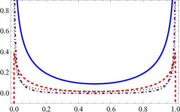
Figure 1: The ratios of 𝐁^​[Πn]\hat{\mathbf{B}}[\Pi_{n}] to the one-loop correlator LO=x​x¯/2\text{LO}=x\bar{x}/2: asCF𝐁^[Π0]/a_{s}C_{F}\hat{\mathbf{B}}[\Pi_{0}]/LO (solid blue line), as2CFβ0𝐁^[Π1]/a_{s}^{2}C_{F}\beta_{0}\hat{\mathbf{B}}[\Pi_{1}]/LO (dashed red line), asCF(asβ0)2𝐁^[Π2]/a_{s}C_{F}(a_{s}\beta_{0})^{2}\hat{\mathbf{B}}[\Pi_{2}]/LO (dotted green line), and asCF(asβ0)3𝐁^[Π3]/a_{s}C_{F}(a_{s}\beta_{0})^{3}\hat{\mathbf{B}}[\Pi_{3}]/LO (dash-dotted purple line). All curves are for the case of l=0l=0, αs​(μ2=1​ GeV2)≈0.49\alpha_{s}(\mu^{2}=1\text{ GeV}^{2})\approx 0.49.

Figure 1 shows several lowest-order contributions to meson DAs in Eq. (3) given by the Borel transform (25) of Eqs. (5)–(7). These curves exhibit different behaviors for the intermediate values of xx, where they decrease sequentially from LO to N4LO, and at the endpoints, where their ratios become singular. The vicinity of endpoints is quantitatively important for the form factors of the mesons considered. Therefore, it makes sense to look at two integral characteristics of the correlators 𝐁^​[Πn​(x,0¯,L)]\hat{\mathbf{B}}[\Pi_{n}(x,\underline{0};L)], their zeroth 𝐁^​[Πn​(0¯,0¯,L)]\hat{\mathbf{B}}[\Pi_{n}(\underline{0},\underline{0};L)] and inverse 𝐁^​[Πn​(−1¯,0¯,L)]\hat{\mathbf{B}}[\Pi_{n}(\underline{-1},\underline{0};L)] moments. They are mostly influenced by intermediate and near-endpoint values of the xx-dependent correlator, respectively.

II.2 The zeroth moment Πn​(0¯,0¯,L)\Pi_{n}(\underline{0},\underline{0};L).

The derivative of the zeroth moment Π˙n​(0¯,0¯,L)\dot{\Pi}_{n}(\underline{0},\underline{0};L) is proportional to the Adler function D⁡(as)D(a_{s}) of QCD. The corresponding exponential generating function (A→u)(A\to u) reads

𝐁~​Π˙​(u)\displaystyle\mathbf{\tilde{B}}\dot{\Pi}(u) ≡∑n⩾0unn!​Π˙n​(0¯,0¯,L)\displaystyle{}\equiv\sum_{n\geqslant 0}\frac{u^{n}}{n!}\dot{\Pi}_{n}(\underline{0},\underline{0};L)
=2​eu​Lc3​(1+u)​(2+u)[Φ(−1,2,1−u)\displaystyle{}=\frac{2e^{uL_{c}}}{3(1+u)(2+u)}\Big[\Phi(-1,2,1-u)
= 2eu Lc3(1+u)(2+u)[ −Φ(−1,2,3+u)],\displaystyle\hphantom{{} = \frac{2e^{u L_{c}}}{3(1+u)(2+u)} \Big[ }{}-\Phi(-1,2,3+u)\Big], (11)

where the function Φ\Phi is Lerch’s transcendent. Using the identity

Φ⁡(−1,2,z)=14​[ψ1​(z/2)−ψ1​((z+1)/2)],\displaystyle\Phi(-1,2,z)=\frac{1}{4}\left[\psi_{1}\left(z/2\right)-\psi_{1}\left((z+1)/2\right)\right], (12)

where ψ1\psi_{1} is the trigamma function, one can arrive at other forms for 𝐁~​Π˙​(u)\mathbf{\tilde{B}}\dot{\Pi}(u) Mikhailov and Volchanskiy 2023; Laenen et al. 2023. Also, it coincides with the Adler function D⁡(as,L)D(a_{s},L) from Ball et al. 1995 for n=2, 3n=2,\,3 and with the all-order result for D⁡(as,L)D(a_{s},L) from Broadhurst 1993; Broadhurst and Kataev 1993. The behavior of the Borel transform 𝐁^​[Πn​(0¯,0¯,L)]\hat{\mathbf{B}}[\Pi_{n}(\underline{0},\underline{0};L)] is depicted in Fig. 2. This asymptotic series should be truncated at n=3n=3 where it becomes divergent and bursts into factorial growth at n≃10n\simeq 10.

Refer to caption
Refer to caption
Figure 2: The ratio Rn(N¯)=−asβ0𝐁^[Πn(N¯,0¯;L)]/𝐁^[Πn−1(N¯,0¯;L)]R_{n}(\underline{N})=-a_{s}\beta_{0}\hat{\mathbf{B}}[\Pi_{n}(\underline{N},\underline{0};L)]/\hat{\mathbf{B}}[\Pi_{n-1}(\underline{N},\underline{0};L)]. Top: N=0N=0. Bottom: N=−1N=-1. R0R_{0} is defined as the ratio of 2-loop and 1-loop correlators, R0​(0¯)=3​as​CFR_{0}(\underline{0})=3a_{s}C_{F} and R0​(−1¯)=5​as​CFR_{0}(\underline{-1})=5a_{s}C_{F} Mikhailov and Radyushkin 1989; Mikhailov and Volchanskiy 2020b. Blue squares are for Rn⩽1R_{n}\leqslant 1. All free parameters are the same as in Fig. 1

II.3 The inverse moment Πn​(−1¯,0¯,L)\Pi_{n}(\underline{-1},\underline{0};L)

The two generating functions for the inverse moment can be written Mikhailov and Volchanskiy 2023 as

Πn​(−1¯,0¯,L)=Πn′​(−1¯,0¯,L)+Πn′′​(−1¯,0¯,L),\displaystyle\Pi_{n}(\underline{-1},\underline{0};L)=\Pi^{\prime}_{n}(\underline{-1},\underline{0};L)+\Pi^{\prime\prime}_{n}(\underline{-1},\underline{0};L), (13)
𝐁~​𝐁^​[Π]​(u)\displaystyle\mathbf{\tilde{B}}\hat{\mathbf{B}}[\Pi](u) ≡∑n⩾0unn!​𝐁^​[Πn′​(−1¯,0¯,L)]\displaystyle{}\equiv\sum_{n\geqslant 0}\frac{u^{n}}{n!}\hat{\mathbf{B}}[\Pi^{\prime}_{n}(\underline{-1},\underline{0};L)]
=−eu​Lc2​Γ​(1−u)​(1+u)​(2+u)\displaystyle{}=\frac{-e^{uL_{c}}}{2\Gamma(1-u)(1+u)(2+u)}
= ×[ψ1​(2−u2)−ψ1​(1−u2)],\displaystyle\hphantom{ {}= }{}\times\Bigl[\psi_{1}\left(\frac{2-u}{2}\right)-\psi_{1}\left(\frac{1-u}{2}\right)\Bigr], (14)
∑n⩾0An​𝐁^​[Πn′′​(−1¯,0¯,L)]=1A​∫0Ad​a​F​(−1¯,a),\displaystyle\sum_{n\geqslant 0}A^{n}\hat{\mathbf{B}}[\Pi^{\prime\prime}_{n}(\underline{-1},\underline{0};L)]=\frac{1}{A}\int_{0}^{A}\mathrm{d}aF(\underline{-1},a), (15)

where

F⁡(−1¯CLOSE,\displaystyle F(\underline{-1},{} OPENa)=Γ⁡(4−2​a)6​Γ​(2−a)2​Γ​(3+a)\displaystyle a)=\frac{\Gamma(4-2a)}{6\Gamma(2-a)^{2}\Gamma(3+a)}
×{5+6​a−5​a2Γ⁡(3−a)+(1+2​a)​[ψ⁡(1−a)−ψ⁡(1)]a​Γ​(1−a)}.\displaystyle{}\times\left\{\frac{5+6a-5a^{2}}{\Gamma(3-a)}+\frac{(1+2a)[\psi(1-a)-\psi(1)]}{a\Gamma(1-a)}\right\}.

Figure 2 illustrates the behavior of the sequence 𝐁^​[Πn​(−1¯,0¯,L)]\hat{\mathbf{B}}[\Pi_{n}(\underline{-1},\underline{0};L)] that can be obtained with the help of (25). The series becomes factorially divergent at n=4n=4.

III QCD SR for the π\pi/ρ∥\rho^{\|} DA of the leading twist

The QCD SRs for the pion and longitudinally polarized ρ\rho-meson DAs of the leading twist 2, φπ\varphi_{\pi} and φρ∥\varphi^{\|}_{\rho}, respectively, read Bakulev and Mikhailov 1998; Mikhailov and Stefanis 2021

(fπ)2φπ(x)+(fA1)2φA1(x)e−m2A1/M2\displaystyle\left(f_{\pi}\right)^{2}\varphi_{\pi}(x)+\left(f_{A_{1}}\right)^{2}\varphi_{A_{1}}(x)e^{-m^{2}_{A_{1}}/M^{2}}
=ΦPT​(x,M,s0A)+ΦS​(x,M)+ΔC=defΦπ​(x,M),\displaystyle\!=\!\Phi_{\text{PT}}(x;M;s_{0}^{A})+\Phi_{S}(x;M)+\Delta_{C}\stackrel{{\scriptstyle\text{def}}}{{=}}\!\Phi_{\pi}(x,M), (16a)
(fρ∥)2φρ∥(x)e−m2ρ/M2+(fρ′∥)2φρ′∥(x)e−m2ρ′/M2\displaystyle\left(f^{\|}_{\rho}\right)^{2}\varphi^{\|}_{\rho}(x)e^{-m^{2}_{\rho}/M^{2}}+\left(f^{\|}_{\rho^{\prime}}\right)^{2}\varphi^{\|}_{\rho^{\prime}}(x)e^{-m^{2}_{\rho^{\prime}}/M^{2}}
=ΦPT​(x,M,s0V)−ΦS​(x,M)+ΔC=defΦρ​(x,M),\displaystyle\!=\!\Phi_{\text{PT}}(x;M;s_{0}^{V})-\Phi_{S}(x;M)+\Delta_{C}\stackrel{{\scriptstyle\text{def}}}{{=}}\!\Phi_{\rho}(x,M), (16b)
where ΦS​(x,M)\Phi_{S}(x;M) is the scalar-condensate contribution and
ΦPT(x;M;s0A)=∫0s0Aρpt(x;s)e−s/M2ds,\displaystyle\Phi_{\text{PT}}(x;M;s_{0}^{A})=\int_{0}^{s_{0}^{A}}\rho_{\text{pt}}(x;s)e^{-s/M^{2}}ds,\, (16c)
ΔC=Δ​ΦG​(x,M)+Δ​ΦV​(x,M)+∑i=13Δ​ΦTi​(x,M).\displaystyle\Delta_{C}=\Delta\Phi_{G}(x;M)+\Delta\Phi_{V}(x;M)+\sum_{i=1}^{3}\Delta\Phi_{T_{i}}(x;M). (16d)

In Eqs. (16), φA1\varphi_{A_{1}} and φ∥ρ′\varphi^{\|}_{\rho^{{}^{\prime}}} are the DAs for the next resonances, s0As_{0}^{A} and s0Vs_{0}^{V} are the duality intervals in the axial (for pion) and vector (for ρ\rho meson) channels, respectively. Remarkably, the right-hand side (rhs) Φπ\Phi_{\pi} and Φρ\Phi_{\rho} of QCD SRs (16) for these two channels differ only in sign of the scalar-condensate contribution ΦS\Phi_{S}. The reason for that was discussed in Mikhailov and Stefanis 2021.

The purely perturbative contributions ΦPT​(x,M,s0A)\Phi_{\text{PT}}(x;M;s_{0}^{A}) and ΦPT​(x,M,s0V)\Phi_{\text{PT}}(x;M;s_{0}^{V}) in the rhs of Eqs. (16a) and (16b) can be obtained from higher order corrections to Π⁡(x,L)\Pi(x;L) by integrating the spectral density ρpt​(x,s)=𝐁^𝟐(s→P2)​Π​(x,L)\rho_{\text{pt}}(x;s)=\mathbf{\hat{B}^{2}}_{(s\to P^{2})}\Pi(x;L) in Eq. (16c), see Appendix B. These perturbative terms dominate in the rhs of Eqs. (16a) and (16b) in accordance with the standard practice of processing QCD SR Shifman et al. 1979. The first two terms of ρpt\rho_{\text{pt}} are ss-independent and have been known Ball and Braun 1996; Mikhailov and Radyushkin 1989 for a long time,

ρpt\displaystyle\rho_{\text{pt}} (x,s)=Nc2​π\displaystyle(x;s)=\frac{N_{c}}{2\pi}
×(x​x¯+as​CF​x​x¯​[5−π23+ln2⁡(x¯x)]+…).\displaystyle{}\times\biggl(x\bar{x}+a_{s}C_{\text{F}}x\bar{x}\left[5-\frac{\pi^{2}}{3}+\ln^{2}\left(\frac{\bar{x}}{x}\right)\right]+\ldots\biggr). (17)

In the vicinity of the endpoints x=0x=0 and 1, the scalar condensate ΦS​(x,M)\Phi_{S}(x;M) dominates the nonlocal condensate (NLC) contributions that include condensates Δ​ΦG,V,Ti​(x,M)\Delta\Phi_{G,V,T_{i}}(x;M) Bakulev and Mikhailov 1998; Bakulev et al. 2001; Bakulev et al. 2004a collected in the term ΔC​(x,M)\Delta_{C}(x;M) in Eq. (16d). To estimate the behavior near the endpoints, we take into account only these two dominant terms, ΦPT\Phi_{\text{PT}} and ΦS\Phi_{S}, in the rhs of Eqs. (16a) and (16b), which is represented diagrammatically in Fig. 3.

𝐁^𝟐(s→P2)​Refer to caption+…∼ρpt​(s);𝐁^(M2→P2)​Refer to caption+m.c.\displaystyle\!\mathbf{\hat{B}^{2}}_{(s\to P^{2})}\begin{gathered}\includegraphics[width,bb]{2loop_p}\end{gathered}+\ldots\sim\rho_{\text{pt}}(s);\,\mathbf{\hat{B}}_{(M^{2}\to P^{2})}\begin{gathered}\includegraphics[width,bb]{2loop_np}\end{gathered}+\!\text{m.c.}
Figure 3: Left diagram: the renormalon-chain contribution to the perturbative part of QCD SR, ΦPT\Phi_{\text{PT}}, via the density ρpt\rho_{\text{pt}}. Right diagram: the contribution of asa_{s}-corrections to ΦS​(x,M)\Phi_{S}(x;M) with a pair of nonlocal scalar condensates depicted by two ovals; the hard propagators of the coefficient function with a renormalon-chain are emphasized with thicker lines; m.c. here means the mirror conjugate diagram.

Note, that we apply here the usual factorization approximation for the four-quark condensate. Our estimates will be made under the renormalon-chain approximation for pQCD corrections, or, in other words, in the approximation of large β0​as\beta_{0}a_{s} in both ΦPT\Phi_{\text{PT}} and ΦS\Phi_{S}. Let us call “reduced NLC SRs” those that contain in their rhs of (16) only the dominant terms ΦPT\Phi_{\text{PT}}, ΦS\Phi_{S}, while all other contributions are neglected.

III.1 Effects of renormalon-chain corrections to pion DA

With growing powers of β0​as\beta_{0}a_{s}, the bubble-chain corrections lead to “swelling” of the perturbative part ΦPT\Phi_{\text{PT}} of DA φπ\varphi_{\pi} at the endpoints, which is shown in the top panel of Fig. 4 in comparison with the leading-order contribution — the asymptotic ΦAs=6​x​x¯\Phi_{\text{As}}=6x\bar{x}. We restrict ourselves to considering orders up to as​(as​β0)3a_{s}(a_{s}\beta_{0})^{3} (the next order as​(as​β0)4a_{s}(a_{s}\beta_{0})^{4} does not change the result significantly) for which the series convergence stays good enough and the series does not yet succumb to factorial growth, see the discussion of Fig.2 in Secs II.2–II.3.

Refer to caption
Refer to caption
Figure 4: Top: the perturbative part ΦPT\Phi_{\text{PT}} of the rhs of NLC SR up to as​(as​β0)3a_{s}(a_{s}\beta_{0})^{3} (solid blue line) in comparison with ΦAs​(x)\Phi_{\text{As}}(x) (dashed red line). Bottom: the rhs of NLC SR, Φπ\Phi_{\pi}, is the sum of the condensate and perturbative contributions up to as​(as​β0)3a_{s}(a_{s}\beta_{0})^{3} for the Borel parameter M2M^{2} in the interval [M−2=0.5[M^{2}_{-}=0.5 (blue line), M+2=1.5M^{2}_{+}=1.5 (red line)] GeV2 at its lower and upper bounds.

At the same time, the corrections to the NLC part ΦS​(x,M)\Phi_{S}(x;M) have the opposite effect, see top panel of Fig. 5 — they alleviate the swelling of the perturbative part ΦPT\Phi_{\text{PT}}. The final result of this mutual compensation in the sum ΦPT​(x,M)+ΦS​(x,M)\Phi_{\text{PT}}(x;M)+\Phi_{S}(x;M) is illustrated in Fig. 4 (bottom panel). We should mention here that Eqs. (16) should be considered as equalities in a weak sense, i.e., for smooth convolutions of both sides of equations within the stability domain in M2M^{2}. Usually, such convolutions are chosen as moments (ξ=2​x−1)N(\xi=2x-1)^{N} or x−1x^{-1}, but, in general, it can be any appropriate function of xx. In addition, the rhs of the QCD SR for DA should not be a smooth function of xx, the smoothness of its behavior depends on a certain model for NLC, see, e.g., discussion in Mikhailov and Stefanis 2021. We use here the simplest Gaussian model for the NLC Mikhailov and Radyushkin 1986; Mikhailov and Radyushkin 1989; Bakulev and Mikhailov 1998 that introduces a single parameter for nonperturbative QCD vacuum, an average virtuality of vacuum quarks ⟨kq2⟩=λq2≡⟨q¯​D2​q⟩/⟨q¯​q⟩|μ02≃1​GeV2\langle k_{q}^{2}\rangle=\lambda_{q}^{2}\equiv\langle\bar{q}D^{2}q\rangle/\langle\bar{q}q\rangle\Big|_{\mu_{0}^{2}\simeq 1\text{GeV}^{2}} at λq2≈0.45\lambda^{2}_{q}\approx 0.45 GeV2 Mikhailov et al. 2021. This model ignores any (still speculative) details of vacuum quark-gluon distributions at the cost of finite discontinuous contributions to the rhs of NLC SR, see the behavior of solid blue/red curves for ΦS​(x,M)\Phi_{S}(x;M) in Fig. 5 (top). The contribution of ΦS​(x,M)\Phi_{S}(x;M) is comparable to ΦPT​(x,M)\Phi_{\text{PT}}(x;M) near the lower bound M−2M^{2}_{-} (blue curve) of the stability interval and significantly decreases at the upper bound M+2M^{2}_{+} (red curve). Let us briefly clarify the calculation of ΦS​(x)\Phi_{S}(x) presented as a right diagram in Fig. 3. The ΦS​(x)\Phi_{S}(x) is a convolution of a pair of scalar NLCs and a coefficient function (for details see Mikhailov and Radyushkin 1989; Mikhailov et al. 2010), the latter includes now a renormalized bubble-chain. Due to the Gaussian decay of the scalar NLC, the corresponding Feynman integrals for this convolution are well convergent and do not need to be renormalized. An important calculation of ΦS​(x)\Phi_{S}(x) of the order as​(as​β0)0a_{s}(a_{s}\beta_{0})^{0} was performed in Mikhailov and Radyushkin 1989 (see also Appendix A of Mikhailov et al. 2010) — our calculations are similar to those. The key integrals for the bubble-chain inclusion in the gluon line of the coefficient function are presented in Appendix C.

Our goal here is to estimate how the QCD corrections affect the behavior of DA at the vicinity of endpoints rather than the whole profile of DA. Moreover, extending the analyses to moderate values of the Bjorken variable would require taking into account the other condensates Δ​ΦG,V,Ti​(x,M)\Delta\Phi_{G,V,T_{i}}(x;M), which are numerically significant somewhere in the middle of the interval of xx. So one can expect that the profile of the “true” pion DA lies somewhere within the yellow region between the blue (at M2=M−2M^{2}=M^{2}_{-}) and red (at M2=M+2M^{2}=M^{2}_{+}) bounds in Fig. 4(bottom) (with some uncertainty in the middle of the xx-interval). The incline of DA near the endpoints varies22 2 For this estimate we have used the technique of average incline elaborated in Mikhailov et al. 2010 from 6 to 7. The inverse moment ⟨x−1⟩π\langle x^{-1}\rangle_{\pi}, an important integral characteristic of Φπ\Phi_{\pi}, is

⟨x−1⟩π≡∫01Φπ​(x,M)​d​xx≈3.4​ for ​M2∈[M−2,M+2].\langle x^{-1}\rangle_{\pi}\equiv\int_{0}^{1}\Phi_{\pi}(x;M)\frac{dx}{x}\approx 3.4\text{ for }M^{2}\in[M^{2}_{-},M^{2}_{+}]. (18)

This estimate of ⟨x−1⟩π\langle x^{-1}\rangle_{\pi} seems reasonable because the inverse moment is mostly formed by the behavior of DA near the left endpoint. The estimate in (18) is only a bit higher than the previous ones obtained in NLC SR Bakulev et al. 2001 and lies within the acceptable region of the phenomenological analysis of the pion transition form factor (TFF) Bakulev et al. 2004b.

III.2 Effects of renormalon-chain corrections to DA φρ∥\varphi^{\|}_{\rho}

For the case of ρ∥\rho_{\|} DA that is determined from the NLC SR in the vector channel, the 4-quark NLC contribution ΦS\Phi_{S} comes with the opposite sign relative to the pion case, which leads to the relation Mikhailov and Stefanis 2021

φρ∥​(x)≈[φπ​(x)−2fπ2​ΦS​(x,M)+ΔA1​ρ′​(x,M)]​eC⁡(M),\displaystyle\varphi_{\rho}^{\|}(x)\approx\left[\varphi_{\pi}(x)-\frac{2}{f_{\pi}^{2}}\Phi_{S}(x,M)\!+\!\Delta_{A_{1}\rho^{\prime}}(x,M)\right]e^{C(M)}, (19)

where

C⁡(M)=mρ2M2+ln⁡(fπ2/fρ2),\displaystyle C(M)=\frac{m_{\rho}^{2}}{M^{2}}+\ln\left(f_{\pi}^{2}/f_{\rho}^{2}\right), (20)
ΔA1​ρ′​(x,M)=\displaystyle\Delta_{A_{1}\rho^{\prime}}(x,M)={} (fA1fπ)2e−mA12/M2φA1(x)\displaystyle\left(\frac{f_{A_{1}}}{f_{\pi}}\right)^{2}e^{-m_{A_{1}}^{2}/M^{2}}\varphi_{A_{1}}(x)
−(fρ′fπ)2e−mρ′2/M2φρ′(x).\displaystyle{}-\left(\frac{f_{\rho^{\prime}}}{f_{\pi}}\right)^{2}e^{-m_{\rho^{\prime}}^{2}/M^{2}}\varphi_{\rho^{\prime}}(x). (21)

The symbol “approximately equal” in Eq. (19) means that we suppose ΦPT​(x,M,s0A)≈ΦPT​(x,M,s0V)\Phi_{\text{PT}}(x;M;s_{0}^{A})\approx\Phi_{\text{PT}}(x;M;s_{0}^{V}) for the purely perturbative parts in both channels. The term ΔA1​ρ′\Delta_{A_{1}\rho^{\prime}} is determined by the difference of the contributions of higher resonances in the phenomenological parts of QCD SR for the axial and vector channels.

Keeping only the contribution ΦPT​(x,M)−ΦS​(x,M)\Phi_{\text{PT}}(x;M)-\Phi_{S}(x;M) (reduced NLC SR) in the rhs of (16b), one gets the profile of φρ∥​(x)\varphi_{\rho}^{\|}(x) that becomes wider near the endpoints. This endpoint “swelling” of the φρ∥​(x)\varphi_{\rho}^{\|}(x) profile is seen clearly in Fig. 5 (bottom panel). This effect can be traced back also in the representation (19) for φρ∥​(x)\varphi_{\rho}^{\|}(x) through φπ​(x)\varphi_{\pi}(x).

Refer to caption
Refer to caption
Figure 5: Top: NLC scalar condensate ΦS\Phi_{\text{S}} up to as​(as​β0)3a_{s}(a_{s}\beta_{0})^{3} for the parameter M2M^{2} in the interval [M−2=0.5[M^{2}_{-}=0.5 (blue line), M+2=1.5M^{2}_{+}=1.5 (red line)] GeV2. Bottom: the rhs of NLC SR for φρ∥\varphi_{\rho}^{\|}, Eq. (19) up to as​(as​β0)3a_{s}(a_{s}\beta_{0})^{3} in the interval [M−2[M^{2}_{-}, M+2]M^{2}_{+}] GeV2.

The incline of the ρ∥\rho^{\|} meson DA near the endpoints is certainly larger than for the pion DA and averages between 9 and 12 with the value of the inverse moment being ⟨x−1⟩ρ≈3.8\langle x^{-1}\rangle_{\rho}\approx 3.8.

Here it is impossible to reliably estimate the moments ⟨ξn⟩\langle\xi^{n}\rangle, ξ=x−x¯\xi=x-\bar{x} of π\pi and ρ∥\rho^{\|} DAs due to the fact that the reduced NLC SR neglects some of the condensate contributions, but we can still suggest inequalities for the moments. The significant swelling effect near the endpoints should lead to the obvious inequalities

⟨ξ2⟩ρ∥>⟨ξ2⟩π>⟨ξ2⟩As=15,\langle\xi^{2}\rangle_{\rho^{\|}}>\langle\xi^{2}\rangle_{\pi}>\langle\xi^{2}\rangle_{\text{As}}=\frac{1}{5}, (22)

and, therefore,

a2ρ∥>a2π>0,a_{2}^{\rho^{\|}}>a_{2}^{\pi}>0, (23)

where a2Ma_{2}^{\text{M}} is the 2nd Gegenbauer moment of DA of a meson M. Since the omitted contribution ΔC\Delta_{C} in the rhs of the NLC SR (16) is the same for both channels, it does not violate the inequalities. The results of lattice calculations Braun et al. 2017; Bali et al. 2019 support the conclusion (23),

a2ρ∥=0.132​(27)​ Braun et al. 2017>a2π=0.116​(20)​ Bali et al. 2019,\displaystyle a^{\rho^{\|}}_{2}=0.132(27)\text{ \cite[cite]{\@@bibref{Authors Phrase1YearPhrase2}{Braun:2016wnx}{\@@citephrase{(}}{\@@citephrase{)}}}}>a^{\pi}_{2}=0.116(20)\text{ \cite[cite]{\@@bibref{Authors Phrase1YearPhrase2}{Bali:2019dqc}{\@@citephrase{(}}{\@@citephrase{)}}}}, (24)
OPENOPENwhile​a2π​ (LattQCD Bali et al. 2019)≈a2π​ (SR Mikhailov et al. 2021)\displaystyle\text{while}\,a^{\pi}_{2}\text{ (LattQCD \cite[cite]{\@@bibref{Authors Phrase1YearPhrase2}{Bali:2019dqc}{\@@citephrase{(}}{\@@citephrase{)}}}})\approx a^{\pi}_{2}\text{ (SR \cite[cite]{\@@bibref{Authors Phrase1YearPhrase2}{Mikhailov:2021znq}{\@@citephrase{(}}{\@@citephrase{)}}}})

at μLatt2=4\mu_{\text{Latt}}^{2}=4 GeV2, λq2≈0.45\lambda^{2}_{q}\approx 0.45 GeV2. Note that the previous versions of NLC SR for DAs of π\pi and ρ∥\rho^{\|} Mikhailov and Stefanis 2021; Pimikov et al. 2014 yielded an opposite hierarchy of the moments, a2ρ∥=0.032​(46)<a2π=0.149−0.043+0.052​(at​μ2=1CLOSEa^{\rho^{\|}}_{2}=0.032(46)<a^{\pi}_{2}=0.149^{+0.052}_{-0.043}\,(\text{at}\,\mu^{2}\!\!=\!1GeV2). The contributions of the orders as​(as​β0)na_{s}(a_{s}\beta_{0})^{n}, n=2n=2, 3 to the dominant components of SRs reverse this situation – allowance for the renormalon-chain effects in the reduced NLC SRs of Eq. (16) provides a new estimate for a2ρ∥a^{\rho^{\|}}_{2} (in the same frame as for a2πa^{\pi}_{2}) that complies with the hierarchy (23) suggested by lattice QCD:

a2ρ∥≈0.15>a2π≈0.07​ at ​μ2=1​ GeV2.a^{\rho^{\|}}_{2}\approx 0.15>a^{\pi}_{2}\approx 0.07\text{ at }\mu^{2}=1\text{ GeV}^{2}.

Let us emphasize that we insist on the validity of inequality (23) for a2Ma_{2}^{\text{M}}, M=π\text{M}=\pi and ρ∥\rho_{\|}, per se, rather than on the precise values of the moments which serve only as an illustration here. To obtain well-grounded estimates of the moments a2Ma_{2}^{\text{M}} one needs the standard treatment of the complete NLC SRs (16).

IV Conclusion

(i) Taking into account renormalon-chain corrections of any order as​(as​β0)na_{s}\left(a_{s}\beta_{0}\right)^{n} in pQCD, we have calculated the correlator Π⁡(x,0¯,L)\Pi(x,\underline{0};L) of two vector quark currents, with one of the currents being nonlocal, which makes the correlator a function of the Bjorken fraction xx. The generating functions for this correlator and some of its moments have been constructed. The zeroth and inverse Mellin moments of the correlator have been obtained for any order nn. The zeroth moment as well as some other fixed-order special cases agree with all previous calculations in the literature.

The correlator Π⁡(x,0¯,L)\Pi(x,\underline{0};L) at any fixed order nn can be expressed in terms of harmonic polylogarithms of weight not higher than n+3n+3. Investigating the asymptotic series in as​(as​β0)na_{s}\left(a_{s}\beta_{0}\right)^{n} for the moments of the correlator, we found that these series should be truncated at n=3n=3 or 4.

(ii)These radiative corrections to perturbative and condensate parts of QCD SR for pion distribution amplitude, φπ​(x)\varphi_{\pi}(x), do not change the behavior of φπ​(x)\varphi_{\pi}(x) at the endpoints x=0x=0 and 1 significantly. Although these changes looks visible and corresponding incline is a bit higher now – up to 77. But this effect cannot disturb the agreement of previous calculations of transition form factor and the phenomenological processing of the data process γ+γ∗→π0\gamma+\gamma^{*}\to\pi^{0} Bakulev et al. 2004b; Mikhailov et al. 2021.

(iii) The same class of radiative corrections to the distribution amplitude of longitudinally polarized ρ\rho-meson, φρ∥​(x)\varphi_{\rho}^{\|}(x), drastically changes the behavior of the DA near the endpoints in such a way that leads to the inequality ⟨ξ2⟩ρ∥>⟨ξ2⟩π\langle\xi^{2}\rangle_{\rho^{\|}}>\langle\xi^{2}\rangle_{\pi} (a2ρ∥>a2π>0a_{2}^{\rho^{\|}}>a_{2}^{\pi}>0). This inequality agrees with the results of lattice calculations in Braun et al. 2017; Bali et al. 2019.

Appendix A BOREL TRANSFORM 𝐁^\mathbf{\hat{B}}

We used the standard form of the Borel transform for QCD SR, see e.g. in Shifman et al. 1979, it reads 𝐁^(M2→P2)​[f​(t)]\hat{\mathbf{B}}_{\scriptstyle{(M^{2}\to P^{2})}}[f(t)] and manifests itself as the limit of a series of derivatives of the function f⁡(t)f(t) for t=P2/μ2t=P^{2}/\mu^{2} (μ2\mu^{2} – normalization scale)

𝐁^(M2→P2)​[f⁡(t)]≡𝐁^​[f⁡(t)]​(M2)=d​e​flimP2=n​M2n→∞(−t)nΓ⁡(n)​dnd​tn​[f⁡(t)].\displaystyle\!\!\!\!\!\hat{\mathbf{B}}_{\scriptscriptstyle{(M^{2}\to P^{2})}}[f(t)]\!\equiv\!\mathbf{\hat{B}}\left[f(t)\right]\!\!(M^{2})\!\stackrel{{\scriptstyle def}}{{=}}\!\!\lim_{\begin{subarray}{c}\scriptscriptstyle{P^{2}=nM^{2}}\\ \scriptscriptstyle{n\to\infty}\end{subarray}}\frac{(-t)^{n}}{\Gamma(n)}\frac{\mathrm{d}^{n}}{\mathrm{d}t^{n}}\left[f(t)\right]. (25)

We emphasize that the Borel transformation 𝐁^(M2→P2)\mathbf{\hat{B}}_{\scriptscriptstyle{(M^{2}\to P^{2})}}, acts on the argument P2P^{2}, this differs from the images of 𝐁~\mathbf{\tilde{B}} (the inverse Laplace transform) acting on the powers of asa_{s} (or the constant A∼asA\sim a_{s}) of the perturbation theory series, the latter have been summed and discussed here in Sec. II.2, II.3. A number of useful formulae for the 𝐁^\hat{\mathbf{B}} are presented below that are based on the definition (25)

𝐁^​[exp⁡(−P2μ2​a)]\displaystyle\!\!\!\!\mathbf{\hat{B}}\left[\exp\left(-\frac{P^{2}}{\mu^{2}}a\right)\right]\! =\displaystyle= δ⁡(1−M2μ2​a).\displaystyle\!\delta\left(1-\frac{M^{2}}{\mu^{2}}a\right). (26)

Based on (26) one can derive

⇒𝐁^​[(μ2P2)n]\displaystyle\Rightarrow\mathbf{\hat{B}}\left[\left(\frac{\mu^{2}}{P^{2}}\right)^{n}\right] =\displaystyle= 1Γ⁡(n)​(μ2M2)n,\displaystyle\frac{1}{\Gamma(n)}\left(\frac{\mu^{2}}{M^{2}}\right)^{n}, (27a)
𝐁^​[ea​L]\displaystyle\mathbf{\hat{B}}\left[e^{aL}\right] =\displaystyle= −a​ea​lΓ⁡(1−a).\displaystyle-\frac{ae^{al}}{\Gamma(1-a)}. (27b)

Here aa is a constant, e.g. , a=A=−as​β0a=A=-a_{s}\beta_{0} as in Sec.II, L=ln⁡tL\!=\!\ln t, l=ln⁡(M2μ2)l\!=\!\ln\left(\frac{M^{2}}{\mu^{2}}\right). The 𝐁^\mathbf{\hat{B}}–images of radiation logs are:

𝐁^​dd​L=dd​l​𝐁^⇒𝐁^​(dd​L​Π=Π˙)=dd​l​𝐁^​Π;\mathbf{\hat{B}}~\frac{d}{dL}=\frac{d}{dl}~\mathbf{\hat{B}}~~~\Rightarrow~~~\mathbf{\hat{B}}\left(\frac{d}{dL}\Pi=\dot{\Pi}\right)=\frac{d}{dl}~\mathbf{\hat{B}}\Pi; (28)
𝐁^​[lnm⁡(t)]​(M2)=\displaystyle\!\!\!\!\mathbf{\hat{B}}\left[\ln^{m}(t)\right](M^{2})\!= m​(−1)m​[(dd​a)m−1​e−a​lΓ⁡(1+a)]a=0\displaystyle m(-1)^{m}\left[\left(\frac{d}{da}\right)^{m-1}\!\!\!\!\frac{e^{-al}}{\Gamma(1+a)}\right]_{a=0} (29a)
=\displaystyle\!\!\!\!= −m​(lB−dd​a)m−1​e−γE​aΓ⁡(1+a)|a=0;\displaystyle\!\!-m\!\left(l_{B}-\frac{d}{da}\right)^{m-1}\!\!\!\!\frac{e^{-\gamma_{\text{E}}a}}{\Gamma(1+a)}\bigg|_{a=0}\!\!; (29b)

here lB=ln⁡(M2μ2)−γEl_{B}\!=\!\ln\left(\frac{M^{2}}{\mu^{2}}\right)-\gamma_{\text{E}}.

Appendix B EXTRACTION OF SPECTRAL DENSITY ρ⁡(s)\rho(s)

Let us define a “double” Borel transform 𝐁^𝟐(s)≡𝐁^𝟐(s→P2)\mathbf{\hat{B}^{2}}_{(s)}\!\!\equiv\!\mathbf{\hat{B}^{2}}_{\scriptscriptstyle{(\!s\to P^{2}\!)}} to obtain the spectral density ρpt​(s)\rho_{\text{pt}}(s) of Π⁡(L)\Pi(L) that is used in Sec.III for QCD SR,

Π⁡(L)=∫0∞ρpt​(s)​d​ss+P2−subtracted terms,\displaystyle\Pi(L)=\int^{\infty}_{0}\frac{\rho_{\text{pt}}(s)ds}{s+P^{2}}-\text{subtracted terms}, (30a)
M2𝐁^(M2→P2)Π(L)=∫0∞ρpt(s)e−s/M2ds,\displaystyle M^{2}\mathbf{\hat{B}}_{\scriptscriptstyle{(M^{2}\to P^{2})}}\Pi(L)=\int^{\infty}_{0}\rho_{\text{pt}}(s)e^{-s/M^{2}}ds, (30b)
𝐁^𝟐(s)​Π​(L)≡1s​𝐁^(𝟏𝐬→σ)​[1σ​𝐁^(𝟏σ→𝐏𝟐)​Π​(L)]=ρpt​(s),\displaystyle\mathbf{\hat{B}^{2}}_{(s)}\Pi(L)\!\equiv\!\frac{1}{s}\mathbf{\hat{B}_{(\frac{1}{s}\to\sigma)}}\!\left[\frac{1}{\sigma}\mathbf{\hat{B}_{(\frac{1}{\sigma}\to P^{2})}}\Pi(L)\right]\!=\!\rho_{\text{pt}}(s), (30c)

where σ\sigma is an intermediate variable. One obtains for every power LnL^{n} in Π⁡(L)\Pi(L) the contribution to ρpt​(s)\rho_{\text{pt}}(s) as a polynomial in ls=ln⁡(s)l_{s}=\ln(s):

𝐁^𝟐(s)​Ln\displaystyle\mathbf{\hat{B}^{2}}_{(s)}L^{n} =\displaystyle= (ls−dd​ν)n​[sin⁡(π​ν)π]|ν=0,\displaystyle\left(l_{s}-\frac{d}{d\nu}\right)^{n}\left[\frac{\sin(\pi\nu)}{\pi}\right]\bigg|_{\nu=0}, (31)
𝐁^𝟐(s)​[ea​L]\displaystyle\mathbf{\hat{B}^{2}}_{(s)}\left[e^{aL}\right] =\displaystyle= −ea​ls​sin⁡(π​a)π.\displaystyle-\displaystyle e^{al_{s}}\,\frac{\sin(\pi a)}{\pi}. (32)
nn 0 1 2 3 4 5
𝐁^𝟐(s)​Ln\mathbf{\hat{B}^{2}}_{(s)}L^{n} 0 −1-1 −2​ls-2l_{s} π2−3​ls2\pi^{2}-3l_{s}^{2} 4​ls​π2−4​ls34l_{s}\pi^{2}-4l_{s}^{3} −π4+10​π2​ls2−5​ls4-\pi^{4}+10\pi^{2}l_{s}^{2}-5l_{s}^{4}

The key element of the perturbative contribution in the “theoretical part” (rhs) of the SR is the integration of lnj⁡(s)\ln^{j}(s) from (31),

∫0s0ρpt(s)e−s/M2ds⇒M2∫0s0/M2lnj(M2t)e−tdt.\displaystyle\int^{s_{0}}_{0}\rho_{\text{pt}}(s)e^{-s/M^{2}}ds\Rightarrow M^{2}\int_{0}^{s_{0}/M^{2}}\ln^{j}(M^{2}t)e^{-t}dt\,. (33)

Taking into account the main terms of the structure of the correlator after summation, i.e. , the terms of the generating functions for Π′\Pi^{\prime} and Π′′\Pi^{\prime\prime} in Secs. II (see the terms in braces below), we present the results for these functions and their different derivatives where aa is a constant,

ρpt​(s)\displaystyle\rho_{\text{pt}}(s) ∝𝐁^𝟐(s)​{exp⁡(a​L)a,L}={−exp⁡(a​ls)​sin⁡(π​a)π​a,−1},\displaystyle\propto\mathbf{\hat{B}^{2}}_{(s)}\Big\{\frac{\exp{(aL)}}{a},L\Big\}=\Big\{-\exp{(al_{s})}\frac{\sin(\pi a)}{\pi a},\,-1\Big\}\,, (34)
𝐁^​Π​(L)\displaystyle\mathbf{\hat{B}}\Pi(L) ∝𝐁^​{exp⁡(a​L)a,L}={−exp⁡(a​l)Γ⁡(1−a),−1},\displaystyle\propto\mathbf{\hat{B}}\Big\{\frac{\exp{(aL)}}{a},\,L\Big\}=\Big\{-\frac{\exp{(al)}}{\Gamma(1-a)},\,-1\Big\}\,, (35)
Π˙​(L)\displaystyle\dot{\Pi}(L) ∝dd​L​{exp⁡(a​L)a,L}={exp⁡(a​L),1}.\displaystyle\propto\frac{d}{dL}\Big\{\frac{\exp{(aL)}}{a},L\Big\}=\Big\{\exp{(aL)},1\Big\}. (36)

Appendix C ΦS\Phi_{S} INTEGRALS

The zeroth-order calculation as​(as​β0)0a_{s}(a_{s}\beta_{0})^{0} of the coefficient function for ΦS\Phi_{S},discussed in detail in Mikhailov and Radyushkin 1989 (see also Appendix A in Mikhailov et al. 2010), was performed for the correlator of the initial two-fold form ΠS​(x,y)\Pi_{S}(x,y). For this two-fold form, the contribution ΠS(n)​(x,y)\Pi^{(n)}_{S}(x,y) with a nn-bubble chain looks most evident as a term of geometric progression

𝐁^​ΠS(n)​(x,y)\displaystyle\mathbf{\hat{B}}\Pi^{(n)}_{S}(x,y) ∼\displaystyle\sim (as​β0)n​𝐒^⁡f⁡(x,y)​[ln⁡(Δ¯y−x−1)−ln⁡(δ2μ02)−c]n;\displaystyle(a_{s}\beta_{0})^{n}\mathop{\hat{\mathbf{S}}}f(x,y)\left[\ln\left(\frac{\bar{\Delta}}{y-x}-1\right)-\ln\left(\frac{\delta^{2}}{\mu_{0}^{2}}\right)-c\right]^{n}; (38)
Δ=δ2M2;Δ¯=1−Δ;δ2=λq22;μ02=μ2​eγE;c=−53;\displaystyle\Delta=\frac{\delta^{2}}{M^{2}};~\bar{\Delta}=1-\Delta;~\delta^{2}=\frac{\lambda_{q}^{2}}{2};~\mu_{0}^{2}=\mu^{2}e^{\gamma_{E}};~c=-\frac{5}{3};
f⁡(x,y)\displaystyle f(x,y) =\displaystyle= 169​π​⟨αs​q¯​q⟩2δ4​Δ¯​x¯​yy−x+Δ​θ​(Δ¯>y−x)​θ​(y>Δ¯)​θ​(y>x)​θ​(Δ>x).\displaystyle\frac{16}{9}\pi\frac{\langle\sqrt{\alpha_{s}}\bar{q}q\rangle^{2}}{\delta^{4}\bar{\Delta}}\frac{\bar{x}y}{y-x+\Delta}\theta(\bar{\Delta}>y-x)\theta(y>\bar{\Delta})\theta(y>x)\theta(\Delta>x). (39)

Finally, we integrate over yy to obtain the contribution to ΠS​(x,0¯)∼ΦS​(x)\Pi_{S}(x,\underline{0})\sim\Phi_{S}(x). The partial contribution ΦS(n)\Phi^{(n)}_{S} of the order (as​β0)n(a_{s}\beta_{0})^{n} to ΦS\Phi_{S} reads

ΦS(n)​(x)\displaystyle\Phi^{(n)}_{S}(x) =\displaystyle= (as​β0)n​169​π​⟨αs​q¯​q⟩2δ4​Δ¯​θ​(1>2​Δ)​θ​(Δ>x)​x¯​∫Δ¯Δ¯+xyy−x+Δ​[ln⁡(Δ¯y−x−1)−ln⁡(δ2μ02)−c]n​𝑑y\displaystyle(a_{s}\beta_{0})^{n}\frac{16}{9}\pi\frac{\langle\sqrt{\alpha_{s}}\bar{q}q\rangle^{2}}{\delta^{4}\bar{\Delta}}\theta(1>2\Delta)\theta(\Delta>x)\bar{x}\int^{\bar{\Delta}+x}_{\bar{\Delta}}\frac{y}{y-x+\Delta}\left[\ln\left(\frac{\bar{\Delta}}{y-x}-1\right)-\ln\left(\frac{\delta^{2}}{\mu_{0}^{2}}\right)-c\right]^{n}\,dy (40)
+(x→x¯)\displaystyle{}+(x\to\bar{x})

The functions of the highest transcendence that appear in ΦS(n)​(x)\Phi^{(n)}_{S}(x) from Eq. (40) are the polylogarithms of weight n+1n+1,

Lin+1⁡(−xΔ¯−x),Lin+1⁡(−x​ΔΔ¯−x),(x↔x¯)\mathop{\mathrm{Li}_{n+1}}\left(-\frac{x}{\bar{\Delta}-x}\right),\mathop{\mathrm{Li}_{n+1}}\left(-\frac{x\Delta}{\bar{\Delta}-x}\right),(x\leftrightarrow\bar{x}) (41)

References

  • Bakulev and Mikhailov (1998) A. P. Bakulev and S. V. Mikhailov, Phys. Lett. B436, 351 (1998), eprint hep-ph/9803298.
  • Mikhailov and Stefanis (2021) S. V. Mikhailov and N. G. Stefanis, Phys. Rev. D 104, 096013 (2021), eprint 2106.15522.
  • Mikhailov and Volchanskiy (2020a) S. V. Mikhailov and N. Volchanskiy, J. Phys. Conf. Ser. 1435, 012059 (2020a).
  • Mikhailov and Volchanskiy (2023) S. V. Mikhailov and N. Volchanskiy, Phys. Part. Nuclei Lett. 20, 296–299 (2023), eprint 2301.01806.
  • Broadhurst and Grozin (1995) D. J. Broadhurst and A. G. Grozin, Phys. Rev. D 52, 4082 (1995), eprint hep-ph/9410240.
  • Mikhailov and Volchanskiy (2019) S. V. Mikhailov and N. Volchanskiy, JHEP 01, 202 (2019), eprint 1812.02164.
  • Mikhailov (1998) S. V. Mikhailov, Phys. Lett. B 431, 387 (1998), eprint hep-ph/9804263.
  • Mikhailov (2000) S. V. Mikhailov, Phys. Rev. D62, 034002 (2000), eprint hep-ph/9910389.
  • Mikhailov and Volchanskiy (2020b) S. V. Mikhailov and N. Volchanskiy, JHEP 21, 197 (2020b), eprint 2010.03557.
  • Remiddi and Vermaseren (2000) E. Remiddi and J. A. M. Vermaseren, Int. J. Mod. Phys. A 15, 725 (2000), eprint hep-ph/9905237.
  • Laenen et al. (2023) E. Laenen, C. Marinissen, and M. Vonk (2023), eprint 2302.13715.
  • Ball et al. (1995) P. Ball, M. Beneke, and V. M. Braun, Nucl. Phys. B 452, 563 (1995), eprint hep-ph/9502300.
  • Broadhurst (1993) D. J. Broadhurst, Zeitschrift für Physik C 58, 339 (1993).
  • Broadhurst and Kataev (1993) D. J. Broadhurst and A. L. Kataev, Phys. Lett. B 315, 179 (1993), eprint hep-ph/9308274.
  • Mikhailov and Radyushkin (1989) S. V. Mikhailov and A. V. Radyushkin, Sov. J. Nucl. Phys. 49, 494 (1989), Yad. Fiz. 49, 794 (1988), JINR-P2-88-103 (in Russian), URL http://inspirehep.net/record/262441/files/JINR-P2-88-103.pdf.
  • Shifman et al. (1979) M. A. Shifman, A. I. Vainshtein, and V. I. Zakharov, Nucl. Phys. B147, 385 (1979).
  • Ball and Braun (1996) P. Ball and V. M. Braun, Phys. Rev. D 54, 2182 (1996), URL https://link.aps.org/doi/10.1103/PhysRevD.54.2182.
  • Bakulev et al. (2001) A. P. Bakulev, S. V. Mikhailov, and N. G. Stefanis, Phys. Lett. B508, 279 (2001), [Erratum: Phys. Lett. B590, 309 (2004)], eprint hep-ph/0103119.
  • Bakulev et al. (2004a) A. P. Bakulev, S. V. Mikhailov, and N. G. Stefanis, Annalen Phys. 13, 629 (2004a), eprint hep-ph/0410138.
  • Mikhailov and Radyushkin (1986) S. V. Mikhailov and A. V. Radyushkin, JETP Lett. 43, 712 (1986), [Pisma Zh. Eksp. Teor. Fiz. 43, 551 (1986)].
  • Mikhailov et al. (2021) S. V. Mikhailov, A. V. Pimikov, and N. G. Stefanis, Phys. Rev. D 103, 096003 (2021), eprint 2101.12661.
  • Mikhailov et al. (2010) S. V. Mikhailov, A. V. Pimikov, and N. G. Stefanis, Phys. Rev. D82, 054020 (2010), eprint 1006.2936.
  • Bakulev et al. (2004b) A. P. Bakulev, S. V. Mikhailov, and N. G. Stefanis, Phys. Lett. B578, 91 (2004b), eprint hep-ph/0303039.
  • Braun et al. (2017) V. M. Braun et al., JHEP 04, 082 (2017), eprint 1612.02955.
  • Bali et al. (2019) G. S. Bali, V. M. Braun, S. Bürger, M. Göckeler, M. Gruber, F. Hutzler, P. Korcyl, A. Schäfer, A. Sternbeck, and P. Wein, JHEP 08, 065 (2019), JHEP 11, 037 (2020), eprint 1903.08038.
  • Pimikov et al. (2014) A. V. Pimikov, S. V. Mikhailov, and N. G. Stefanis, Few Body Syst. 55, 401 (2014), eprint 1312.2776.