Neutral delay differential equation Kerr cavity model

Over the last two decades, optical frequency combs have found applications in different fields of science and industry including spectroscopy, optical ranging, metrology, searching for exoplanets, microwave photonics and optical communications Cundiff and Ye 2003; Schröder et al. 2019; Picqué and Hänsch 2019; Suh et al. 2019; Trocha et al. 2018; Xue and Weiner 2016. Standard methods of the frequency comb generation are based on the use of mode-locked lasers Jones et al. 2000 and optical microcavities subject to an external coherent injection Del’Haye et al. 2007. One of the most commonly used methods to model Kerr optical cavities is based on the application of the paradigmatic Lugiato-Lefever equation (LLE) Lugiato and Lefever 1987, which is known to exhibit S-shaped branches of continuous wave (CW) solutions as well as dissipative solitons preserving their shape in the course of propagation along the cavity axis and sitting on a constant intensity background. The latter solutions correspond to the so-called temporal cavity solitons (TCSs), which were observed experimentally in optical microresonator frequency comb generators Herr et al. 2014, optical fiber cavities Leo et al. 2010, and mode-locked lasers Grelu and Akhmediev 2012. The LLE based on the mean field approximation is, however, not free from certain shortcomings. In particular, it describes bistable behavior and TCS formation only in the vicinity of a single cavity resonance Chembo and Menyuk 2013; Herr et al. 2014. To overcome this shortcoming the modeling approaches based on the so-called generalized Ikeda map Mc Laughlin et al. 1983; Haelterman et al. 1992; Coen and Haelterman 1997; Coen et al. 2013; Hansson and Wabnitz 2015 and a generalized LLE model with localized injection and losses Kartashov et al. 2017 were developed to describe the appearance of the overlap of multiple nonlinear resonances, multistability of CW solutions, and supersolitons Hansson and Wabnitz 2015. Here we propose an alternative approach to model nonlinear dynamics of an injected Kerr cavity based on second order neutral type delay differential equation (NDDE), which also can be considered as a generalization of the Ikeda map Ikeda 1979. Several DDE models were already used previously to study the influence of chromatic dispersion on the dynamics of laser systems Heuck et al. 2010; Pimenov et al. 2017; Schelte et al. 2019; Schelte et al. 2020; Pimenov et al. 2020; Pimenov and Vladimirov 2022; Seidel et al. 2022. We show that in a certain limit the NDDE model can be reduced to the LLE. We perform linear stability analysis of the NDDE model in the practically important large delay limit and present numerical evidence of the existence of stationary and oscillating dissipative optical solitons in it. We show that beyond the LLE limit the TCSs of the NDDE model are strongly affected by the Cherenkov radiation induced by the high order dispersion. The modeling approach proposed here can be adopted to study the dynamics of solid state and fiber lasers, where the chromatic dispersion of the intracavity media plays an important role in the mechanism of the short pulse generation as well as to investigate the effect of second and higher order dispersion on the characteristics of mode-locking regimes in semiconductor lasers. Furthermore, the NDDE model might be useful to model the coupled-cavity systems such as microcavity optical frequency comb generator pumped by a semiconductor mode-locked light source, which is already successfully modeled by DDE models Vladimirov and Turaev 2005; Vladimirov et al. 2004; Vladimirov and Turaev 2004; Viktorov et al. 2006.

A neutral delay differential equation (NDDE) model of a ring Kerr cavity subject to a coherent optical injection reads:

where $t$ is the time, $A(t)$ is the normalized electric field envelope, $A_{\tau}=A\left(t-\tau\right)$ is the retarded field amplitude with the delay time $\tau$ equal to the linear round-trip time of the cavity. $\alpha$ is the Kerr coefficient, $\kappa$ is the linear intensity attenuation factor per cavity round-trip, $\eta$ is the normalized injection rate, and $\theta$ describes the detuning between the injection frequency and the frequency of a cavity mode. The coefficients $a>0$ and $b$ are responsible for the intracavity dispersion. Note that, as it will be shown below, in the LLE limit only the coefficient $b$ contributes to the second order dispersion, while the parameter $a$ describes the group delay due to the first order dispersion. In the absence of injection and losses, $\eta=0$ and $\kappa=1$, Eq. (1) is similar to the conservative version of the Gires–Tournois interferometer model introduced in Seidel et al. 2022. Similarly to this model Eq. (1) with $\eta=0$ and $\kappa=1$ is symmetric under the transformation $t\to-t$ and $A\to A^{*}$ combined with the time shift and, hence, it is reversible in the non-dissipative limit. Note, however, that unlike the first order NDDE Gires–Tournois interferometer model studied in Seidel et al. 2022 the second order derivative terms responsible for the second order dispersion in the LLE limit are present in Eq. (1), see also Ref. Pimenov and Vladimirov 2022. This is an important difference between Eq. (1) and the model of Ref. Seidel et al. 2022. Note that for $a=b=0$ Eq. (1) becomes similar to the well known Ikeda map Ikeda 1979. The derivation of Eq. (1) is given in the next section together with the derivation of three other versions of the NDDE model including the mean field one. An advantage of the model equation (1) is that in the non-dissipative limit, $\eta=0$ and $\kappa=1$, similarly to the first order NDDE discussed in Seidel et al. 2022 it admits a relatively simple conserved quantity $\partial_{t}W\left(t\right)=0$ with

Therefore this study is mainly focused on the analysis of Eq. (1).

To derive the NDDE model let us consider the schematic representation of a ring Kerr cavity with a pair of thin dispersive elements and two identical Kerr media shown in Fig. 1. The field envelope on the output of the left Kerr medium is given by $A_{2}\left(t+\tau_{1}\right)=A_{1}\left(t\right)e^{i\alpha\left|A_{1}\left(t\right)\right|^{2}/2+i\phi_{1}}$, where $\alpha$ is the Kerr coefficient, $\phi_{1}$ and $\tau_{1}$ are the phase shift and the delay time due to the propagation in the cavity, see Fig. 1(a).

The Fourier transform of the field envelope at the output from a thin dispersive element (phase filter) is given by $\hat{A}_{3}\left(\omega\right)=\hat{f}\left(\omega\right)\hat{A}_{2}\left(\omega\right)$, where $\hat{A}_{2}\left(\omega\right)$ is the Fourier transform of the input field $A_{2}\left(t\right)$ and $\hat{f}\left(\omega\right)=e^{-i\Phi\left(\omega\right)}$ with real $\Phi\left(\omega\right)$, see e. g. Ref. Heuck et al. 2010. Close to $\omega=0$ we can use the expansion

. Taking this relation into account, the electric field envelope $A_{3}$ can be expressed as

where ${\cal F}^{-1}$ is the inverse Fourier transform and the notations $\Phi\left(0\right)\equiv\phi$, $\Phi^{\prime}\left(0\right)\equiv a$, and $\Phi^{\prime\prime}\left(0\right)\equiv-b$ are used. The field amplitude $A_{4}$ is obtained from $A_{3}$ by taking into account time delay $\tau_{2}$ , phase shift $\phi_{2}$, and introducing the injection rate $\eta$, and the intensity attenuation factor $\kappa$ due to the cavity losses. Thus we get

with the one half of the cavity round trip time $\tau/2=\tau_{1}+\tau_{2}$ and the phase shift $\theta/2=-\left(\phi_{1}+\phi+\phi_{2}\right)$.

The field envelope on the input of the left Kerr medium is given by $A_{6}\left(t-\tau_{1}\right)=A_{1}\left(t\right)e^{-i\alpha\left|A_{1}\left(t\right)\right|^{2}/2-i\phi_{1}}$ with $\left|A_{1}\left(t\right)\right|^{2}=\left|A_{6}\left(t-\tau_{1}\right)\right|^{2}$. The Fourier transform of the field envelope $A_{6}$ is given by $\hat{A}_{6}\left(t\right)=\hat{f}\left(\omega\right)\hat{A}_{5}\left(\omega\right)$, which can be rewritten as $\hat{A}_{5}\left(t\right)=\hat{f}^{-1}\left(\omega\right)\hat{A}_{6}\left(\omega\right)=\hat{f}^{*}\left(\omega\right)\hat{A}_{6}\left(\omega\right)$. Hence we get

Therefore, similarly to (4) we obtain

Finally, shifting the time in Eq. (4) by $-\tau$, equating the resulting equation to Eq. (5), and neglecting high order dispersion terms ${\cal O}\left(\partial_{ttt}\right)$ we get

where $A\equiv A_{1}$ and $A_{\tau}=A\left(t-\tau\right)$.

The model (1) can be derived in a similar way to Eq. (6), see Fig. 1(b). Here neglecting the high order dispersions we get:

and

Substituting Eq. (7) into Eq. (8), assuming that $a$, $b$, and $\alpha$ are sufficiently small, and neglecting the ${\cal O}\left(\alpha a\right)$ and ${\cal O}\left(\alpha b\right)$ terms in the exponential we obtain

Similarly, for another half of the cavity, we get

Finally, combining Eqs. (9) and (10) we arrive at the NDDE model (1). The latter equation can be further simplified under the approximation $\alpha a,\alpha b\ll 1$, which was already used above:

In the mean field approximation, where the field amplitude is small, expanding the exponentials in Eq. (III) we get the following equation:

Neutral DDEs (1), (6), (III), and (13) are reversible in the non-dissipative limit $\eta=0$ and $\kappa=1$. This property is similar to that of the LLE, which will be derived from these equations in the next section. As it will be shown in the next section, the parameter $b$ corresponds to the second order dispersion coefficient in the LLE limit. In the absence of dispersion according to Eq. (7) the field amplitude on the output of the dispersive element is defined by

Therefore, the parameter $a$ has the meaning of the group delay introduced by the dispersive element. The inequality $a>0$ follows from the causality principle. As it will be shown below this inequality is the necessary but not sufficient condition of the absence of a spurious instability in the NDDE models.

Note, that a straightforward derivation of the model equation without splitting Kerr and dispersive media into two symmetric parts would result in a “regular” DDE model instead of NDDE:

which is similar to the generalization of the Ikeda map derived in Pimenov and Vladimirov 2022 to describe a Kerr cavity with two spectral filters. After rescaling the time variable $t\to\sqrt{2}at$ the DDE model (14) is transformed into Eq. (12) of Ref. Pimenov and Vladimirov 2022 with the constraint $\sigma=\sqrt{2}$. This constraint, however, contradicts to the applicability condition of the DDE model of Ref. Pimenov and Vladimirov 2022. Below, in Sec. V we show that Eq. (14) with $b\neq 0$ demonstrates a spurious instability in the zero loss and injection limit, $\kappa=1$ and $\eta=0$. This instability is related to a dissipation introduced by the truncation of the series expansion in Eq. (2). On the other hand, in the derivation of the NDDE model (1) we have used two truncations of the two transfer functions and in this case the corresponding dissipative contributions cancel each other.

To conclude this section, we note that the derivation presented here can be trivially generalized by including higher order dispersion terms into the model equation.

Using the multiscale method described in Kolokolnikov et al. 2006 we can derive the same LLE from any one of the four model equations (1), (6), (III), and (13). To be more specific, we choose Eq. (1) and in the large delay limit $\tau=\epsilon^{-1}\gg 1$ rescale the time as $x=\epsilon t$ to get

where $A_{\tau_{1}}=A\left(t-1\right)$. Next, we introduce two time scales $A\left(t\right)=u\left(t_{0},t_{2}\right)$, where $t_{0}=\left(1-\epsilon c_{1}+\epsilon^{2}c_{2}+\dots\right)x$ , $t_{2}=\epsilon^{2}x$, and rescale the parameters as

Substituting these expressions into Eq. (15), collecting the first order terms in $\epsilon$, and using the Fredholm alternative we obtain the following boundary condition

together with the relation $c_{1}=2a$ for the group delay parameter. Finally, collecting the second order terms in $\epsilon$ we get $c_{2}=4a^{2}$ and the LLE model:

Note that Eq. (18) with the boundary condition (17), where the parameter $\theta$ plays the role of the detuning, is able to describe multiple resonances corresponding to different cavity modes. However, it cannot describe the overlap of these resonances. In order to get overlapping resonances and coexisting different solitons one needs to replace distributed injection and losses with the localized ones, as it was proposed in Kartashov et al. 2017. It is seen from Eq. (18) that the coefficient $b$ in front of the second derivative terms is responsible for the second order dispersion in the LLE limit, see also Pimenov and Vladimirov 2022. Therefore, these derivatives cannot be neglected in the model equation.

Using the additional assumption that the detuning is small,

instead of (18) we get the standard LLE describing a vicinity of a single cavity resonance

with the periodic boundary condition $u\left(t_{0},t_{2}\right)=u\left(t_{0}-1,t_{2}\right)$.

Note that, unlike Eqs. (18) and (20) obtained by collecting $\epsilon^{2}$-terms, in Ref. Seidel et al. 2022, where the nonlinear Schrödinger equation (NLSE) was derived from a NDDE without second order derivatives and the external injection, the second and third order dispersion terms appear simultaneously in the oder $\epsilon^{3}$. The NLSE is then obtained by choosing the detuning in such a way that the third order dispersion vanishes. In the conservative limit the LLE (20) also transforms into the NLSE. However, the existence of stable soliton solutions is hardly possible in the full NDDE model near this limit. Since unlike the standard NLSE the NDDE contains the dispersion of all the orders, the next order after the second order dispersion will be the third order one. However, it is well known that the solitons of the NLSE are destroyed by the Cherenkov radiation Karpman 1993a; Akhmediev and Karlsson 1995 in the presence of an arbitrary small third order dispersion term Wai et al. 1990; Elgin 1992; Gordon 1992.

Let us consider the linear equation

obtained by the linearization of the NDDE models with $\kappa=1$ and $\eta=0$ at the trivial solution $A=0.$ Substituting $A\left(t\right)=A_{0}e^{\lambda t}$ into (21) we get the characteristic equation

In the large delay limit using the approach of Ref. Yanchuk and Wolfrum 2010 we substitute $e^{-\lambda\tau}\equiv Y$ into Eq. (22), solve the resulting equation with respect to $Y$, and set $\lambda=i\nu$. Thus, we get the following expression for the pseudo-continuous spectrum in the limit $\tau\to\infty$

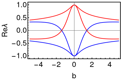
with real $\Psi\left(\nu\right)$. The fact that the pseudo-continuous spectrum of Eq. (21) is purely imaginary is obviously the consequence of the reversibility of this equation, see also Ref. Seidel et al. 2022. However, whether this system exhibits spurious instability depends on the discrete spectrum of the characteristic equation (22). In the large delay limit discrete eigenvalues with positive real parts correspond to small $\left|Y\right|\ll 1$ in the limit $\tau\to\infty$. Therefore, they can be obtained by equating to zero the left hand side of Eq. (22), $1+a\lambda+(a^{2}-ib)\lambda^{2}/2=0$, which gives

The real parts of the eigenvalues $\lambda_{\pm}$ are shown in Fig. 2 as functions of the “second order dispersion coefficient” $b$. It is seen that for $a<0$ one of the two discrete eigenvalues always has a positive real part. This means that Eq. (21) with $a<0$ should demonstrate a spurious instability. For $a>0$ both the eigenvalues $\lambda_{\pm}$ have negative real parts if

Hence, in order to avoid spurious instabilities below we choose $a>0$ in the NDDE models and assume that the inequality (25) is satisfied. Note that positive coefficient $a$ can be rescaled to unity by rescaling the time variable in the model equations.

Substituting $\kappa=1$ and $\eta=0$ into Eq. (14) and linearizing this equation at $A=0$, instead of (23) we get $\lambda\tau=-\ln\left[1+2ia\nu-\left(2a^{2}-ib\right)\nu^{2}\right]+i\theta$. In particular, at $\nu=0$ one obtains

It follows from these relations that for any nonzero $b$ and sufficiently small $\nu$ the curve of the pseudo-continuous spectrum visits the right halfplane of the complex plane. Therefore, in this case one can expect an instability associated with the pseudo-continuous spectrum in the large delay limit.

In this section we study the linear stability of the CW solutions of Eq. (1). The amplitude $A$ of the CW solutions satisfies the equation

Substituting into Eq. (26) $A=\sqrt{I}e^{i\varphi}$, where $I$ and $\varphi$ are the intensity and the phase of the CW solution, and separating real and imaginary parts of the resulting equation we get the following equation for the CW intensity

which is transformed into the corresponding relation of the LLE in the limit (16) and (19). The phase of the CW solution is given by

Nonlinear resonances of CW solutions of Eq. (1) near cusp bifurcations corresponding to different cavity modes are shown in Fig. 3(a).

The saddle-node bifurcations of the CW solutions are defined by the conditions

where $\theta_{\pm}$ with $n=0,\pm 1,\pm 2\dots$ define pairs of saddle-node bifurcation curves originating from the cusp bifurcation points corresponding to different cavity resonances. Figure 3(b) illustrates the coexistence of multiple CW solutions of Eq. (1). It is seen that at sufficiently high injection rates the CW resonances start overlapping. Unlike the resonances shown in Fig. 3(b), the resonances of Eq. (13) with cubic nonlinearity are much more narrow and never overlap. This can be easily understood by noticing that for cubic nonlinearity Eq. (27) transforms into a cubic equation in $I$ having not more than three solutions. Hence, the mean field model (13) does not describe well the dynamics of Eq. (1) beyond the LLE limit. Therefore, below we focus mainly on the model (1), which does not assume the mean field approximation.

To study the linear stability of the CW solution we linearize Eq. (1) around this solution, $A(t)=\left(\sqrt{I}+\delta Ae^{\lambda t}\right)e^{i\varphi}$. Thus we get the following characteristic equation:

where $Y(\lambda)=\exp(-\lambda\tau)$, and the coefficients $c_{0,1,2}$ are polynomoals in $\lambda$:

In the limit of large delay time $\tau\rightarrow\infty$ the eigenvalues of the pseudo-continuous spectrum (PCS) can be represented as $\lambda\approx i\mu+\gamma/\tau$ with real $\mu$ and $\gamma$ Yanchuk and Wolfrum 2010. The pseudo-continuous spectrum is given by the two solution branches of the quadratic equation (28):

Stable CW solutions are characterized by $\gamma\left(\mu\right)<0$ and, in particular, $\gamma\left(0\right)<0$. At the saddle-node (flip) bifurcation point we have $\gamma\left(0\right)=0$ and $Y\left(0\right)=1$ ($\gamma\left(0\right)=0$ and $Y\left(0\right)=-1$), while modulational instability takes place when one or both the branches of pseudo-continuous spectrum are tangent to the imaginary axis at $\mu=\pm\mu_{m}$ with $\left|\mu_{m}\right|>0$.

S-shaped CW curve of Eq. (1) is shown in Fig. 4(a). It is seen that modulational instability takes place on the unstable middle part of the CW curve and destabilizes its upper part. Figures 4(c)-(d) present the real parts of the pseudo-continuous eigenvalues $\gamma\left(\mu\right)$ calculated at the points indicated in 4(a). Figure 4(e) illustrates the location of the modulational instability curve between two saddle-node bifurcations around a single cavity resonance in ($\eta^{2},\theta$)-plane. Finally, Fig. 4(f) illustrates a growing multiplicity of the solutions of Eq. (27) due to the overlap of resonances with increasing the injection rate.

It is important also to check the discrete spectrum of nonlinear CW solutions. The discrete spectrum is defined by the instantaneous part of the model equation and can be obtained by solving the equation $c_{0}=0$ with respect to $\lambda$, where $c_{0}$ is defined by Eqs. (28) and (29). It is seen from Fig. 5 corresponding to $b=(\sqrt{2}+0.01)a^{2}$ that when $b$ exceeds slightly the critical value defined by (25) the lower part of the CW branch can become unstable with respect to the discrete spectrum, see Fig. 5(a). The increase of the CW intensity $I$ has a stabilizing effect on the discrete spectrum. However, as it is seen from Fig. 5(b) the solution of Eq. (1) starting from the upper CW state becomes unbounded in the limit $t\to\infty$. This behavior might be attributed to a spurious instability.

In this section we investigate numerically TCS solutions of the NDDE models using the RADAR5 code written in FORTRAN Guglielmi and Hairer 2001. We start with the delay time $\tau=25$ and the parameter values close to the LLE limit defined by Eqs. (16) and (19) , $\kappa=e^{-2\epsilon^{2}}$, $\alpha=\epsilon^{2}$, $a=\epsilon$, $b=\epsilon^{2}$, $\theta=-3.5\epsilon^{2}$, $\eta=1.855\epsilon^{2}$ with $\epsilon=0.02$. The calculated TCS solution of Eq. (1) is shown in Fig. 6(a) by black line. This soliton is very close to the TCS of the model (6) shown by green line. Dissipative soliton of the LLE (20) is indicated by red dashed line in the same figure for the LLE parameter values obtained using the relations (16) and (19), $k=1$, $\Theta=-3.5$, $\chi=1$, $b=1$, $r=1.855$ in Eq. (20). With increasing $\epsilon$ the soliton profile gets more asymmetric, see Figs.6(c) and (d) obtained with $\epsilon=0.1$. As it is seen in Fig. (d), the soliton tails exhibit slowly decaying oscillations, which can be attributed to the so-called Cherenkov radiation induced by high order dispersion Karpman 1993b; Akhmediev and Karlsson 1995. The Cherenkov radiation amplitude increases with $\epsilon$, see Fig. 6(b) obtained with $\epsilon=0.34$ and eventually destroys the TCS.

The dependence of the TCS peak power on the parameter $\epsilon$ calculated using the models (1) (black line) and (6) (blue line) with exponential nonlinearity, and the model (13) (red line) with cubic nonlinearity is shown in Fig. 7. It is seen that while sufficiently close to the LLE limit, $\epsilon\to 0$, this dependence looks rather smooth, it becomes fast oscillating with the increase of $\epsilon$. Such oscillatory behavior can be explained by the interaction of a TCS with its own tails leading either to constructive or destructive interference due to the presence of Cherenkov radiation. Furthermore, it is seen that the oscillation frequency increases with the decrease of $\epsilon$, which is in agreement with the fact that the frequency of the Cherenkov radiation tends to infinity when the third and/or fourth order dispersion coefficients tend to zero, see e. g. Vladimirov et al. 2018; Vladimirov et al. 2021. Note that the more exact model (6) demonstrates weaker dependence of the TCS peak power on the Cherenkov radiation than Eq. (1). Therefore, Eq. (6) may be more suitable for the description of the system dynamics far away from the LLE limit.

At relatively high values of $\epsilon$ different types of TCS can appear, as it is shown in Fig. 8. Their stability ranges in the parameter space are relatively small, but with $\epsilon=0.722$ can coexist for the same set of parameters.

It is known that the soliton of the LLE can undergo an oscillatory instability with the increase of the injection rate. The NDDE model (1) also shows a similar behavior. Figure 9 illustrates the appearance of undamped oscillations of the soliton peak power for fixed relatively small $\epsilon=0.05$. At higher values of $\epsilon$ there are different types of oscillating TCSs.

To conclude, we have developed a second order NDDE model of a ring dispersive Kerr cavity with a coherent optical injection. Similarly to the first order NDDE model discussed in Seidel et al. 2022 in the non-dissipative limit this model is reversible and has a conserved quantity. In a certain parameter range and under the mean field and large delay approximations the NDDE model can be reduced to the famous LLE model. However, unlike the LLE and similarly to the Ikeda map Haelterman et al. 1992 and generalized LLE Kartashov et al. 2017 Kerr cavity models, the NDDE model is able to describe the overlap of the resonances associated with different cavity modes. We have shown that TCSs can exist in the NDDE model not only close to the LLE limit, but also beyond this limit. In the latter case they are strongly affected by the Cherenkov radiation, which is induced by high order dispersion and eventually destroys the TCS. An important advantage of the NDDE model is that it can be analyzed numerically using standard codes, such as RADAR5 Guglielmi and Hairer 2001 and DDE-biftool Engelborghs et al. 2001. Furthermore, after appropriate modifications this model can be applied to study the effect of chromatic dispersion on the dynamics of mode-locked lasers and other laser systems. The NDDE model might be also useful for the consideration of the coupled-cavity systems, such as an optical microcavity pumped by a semiconductor mode-locked laser modeled by the DDE mode-locking model Vladimirov and Turaev 2005; Vladimirov et al. 2004; Vladimirov and Turaev 2004. This model can be easily extended by including higher order dispersion terms into it.