Precision tracking of massive black hole spin evolution with LISA

Geraint Pratten Email: g.pratten@bham.ac.uk Affiliation: School of Physics and Astronomy, University of Birmingham, Edgbaston, Birmingham, B15 2TT, United Kingdom Affiliation: Institute for Gravitational Wave Astronomy, University of Birmingham, Edgbaston, Birmingham, B15 2TT, United Kingdom Patricia Schmidt Email: p.schmidt@bham.ac.uk Affiliation: School of Physics and Astronomy, University of Birmingham, Edgbaston, Birmingham, B15 2TT, United Kingdom Affiliation: Institute for Gravitational Wave Astronomy, University of Birmingham, Edgbaston, Birmingham, B15 2TT, United Kingdom Hannah Middleton Email: hannahm@star.sr.bham.ac.uk Affiliation: School of Physics and Astronomy, University of Birmingham, Edgbaston, Birmingham, B15 2TT, United Kingdom Affiliation: Institute for Gravitational Wave Astronomy, University of Birmingham, Edgbaston, Birmingham, B15 2TT, United Kingdom Alberto Vecchio Email: av@star.sr.bham.ac.uk Affiliation: School of Physics and Astronomy, University of Birmingham, Edgbaston, Birmingham, B15 2TT, United Kingdom Affiliation: Institute for Gravitational Wave Astronomy, University of Birmingham, Edgbaston, Birmingham, B15 2TT, United Kingdom

August 11, 2026

Abstract

The Laser Interferometer Space Antenna (LISA) will play a vital role in constraining the origin and evolution of massive black holes throughout the Universe. In this study we use a waveform model (IMRPhenomXPHM) that includes both precession and higher multipoles, and full Bayesian inference to explore the accuracy to which LISA can constrain the binary parameters. We demonstrate that LISA will be able to track the evolution of the spins – magnitude and orientation – to percent accuracy, providing crucial information on the dynamics and evolution of massive black hole binaries and the galactic environment in which the merger takes place. Such accurate spin-tracking further allows LISA to measure the recoil velocity of the remnant black hole to better than $100\,\mathrm{km}\,\mathrm{s}^{-1}$ (90% credibility) and its direction to a few degrees, which provides additional important astrophysical information on the post-merger association. Using a systematic suite of binaries, we showcase that the component masses will be measurable at the sub-percent level, the sky area can be constrained to within $\Delta\Omega_{90}\approx 0.01\,\rm{deg}^{2}$ , and the binary redshift to less than $0.01$ .

I Introduction

The Laser Interferometer Space Antenna (LISA) will allow us to observe the mHz gravitational-wave (GW) spectrum. One of the key science goals of the mission is to trace the origin, evolution, and merger history of massive black hole (MBHs) throughout the Universe Klein et al. 2016; Sesana 2021; Amaro-Seoane et al. 2023, where $M\sim 10^{4}-10^{9}M_{\odot}$ . These sources will be detected with large signal-to-noise ratios (SNR), allowing us to precisely measure the mass and spin angular momenta of the constituent black holes.

The population properties of the massive black hole binaries (MBHBs) that will be detected by LISA depends on a wide range of possible evolutionary pathways. Observing and characterising this population will provide vital insight into black hole seed formation, galaxy assembly, and the formation and evolution of structure throughout the Universe Yu and Tremaine 2002; Tanaka and Haiman 2009; Volonteri 2010; Klein et al. 2016; Amaro-Seoane et al. 2023. Whilst there are numerous open issues, there are several mechanisms that are of key importance but are still dominated by large theoretical and observational uncertainties. For example, we have a comparatively poor understanding of the mechanisms that generate the initial black hole seeds at high redshift ( $z\gtrsim 15$ ) and the mechanisms that drive formation of the first protogalaxies. This, in turn, leads to a large uncertainty in the anticipated detection rates and the underlying astrophysical population properties Klein et al. 2016; Barausse et al. 2020; Sesana 2021.

MBHs are known to reside in the centres of galaxies, e.g. Kormendy and Richstone 1995; Ghez et al. 1998; Gebhardt et al. 2000; Ferrarese and Merritt 2000; Schödel et al. 2003; Ferrarese and Ford 2005; Ghez et al. 2008; Genzel et al. 2010; Kormendy and Ho 2013; Akiyama et al. 2019, and there is evidence that some galaxies contain a MBH, even at the early cosmological times probed at high redshift Bañados et al. 2014; Wu et al. 2015; Banados et al. 2018. Coupled with the hierarchical assembly of galaxies through repeated mergers Fakhouri et al. 2010; Giersz et al. 2015; O’Leary et al. 2021; Volonteri et al. 2021, it is anticipated that LISA will observe numerous MBHBs across a wide range of cosmic epochs. However, there is huge uncertainty on our understanding of the astrophysical mechanisms that produced the initial seeds from which they grew. Did they originate from the collapse of heavy population III stars forming in low-metallicity environments (light seeds) Madau and Rees 2001; Heger et al. 2003; Hirano et al. 2014 or from the collapse of large proto-galactic disks (heavy seeds) Haehnelt and Rees 1993; Loeb and Rasio 1994; Bromm and Loeb 2003; Begelman et al. 2006; Lodato and Natarajan 2006; Agarwal et al. 2012? How did these black holes (BHs) subsequently grow? Accretion is an inevitable process and plays a key role in the growth of MBHs Yu and Tremaine 2002; Volonteri and Rees 2006; Ananna et al. 2019. However, there are other mechanisms that can drive the growth of MBHs, such as repeated hierarchical mergers Volonteri et al. 2003; Hopkins et al. 2006; Sesana et al. 2007; Tanaka and Haiman 2009. Observations of MBHBs by LISA will provide us with a unique opportunity to tackle these questions and to constrain the evolutionary pathways responsible for the MBHs observed today.

For a binary of MBHs to merge, efficient mechanisms that dissipate the angular momentum of the system are required. Consequently, our current understanding of massive BH evolution can be broadly divided into distinct phases that are characterized by the astrophysical mechanisms driving angular momentum loss in the binary. The initial phase is primarily driven by dynamical friction caused by the gravitational interaction between the BHs and the surrounding gas and stellar material. Within this phase, the BHs are driven from a separation of approximately $\sim\mathcal{O}(10^{-2}\rm{Mpc})$ to $\sim\mathcal{O}(1\rm{pc})$ Frank and Rees 1976. Below these separations, the dominant mechanism is hardening Frank and Rees 1976; Lightman and Shapiro 1977; Quinlan 1996. Hardening refers to the interaction of fast-orbiting stellar objects and the MBHB, resulting in energy being removed from the system. If the galactic host is sufficiently gas rich, a high-density circumbinary disk can form, leading to additional hardening of the binary through viscous dissipation Begelman et al. 1980; Gould and Rix 2000; Escala et al. 2005. At scales below the hardening separation, e.g. Vasiliev et al. 2014, GW emission becomes the dominant mechanism driving the inspiral of the binary Peters and Mathews 1963. However, depending on the physical properties of the BHs, and the environment of their galactic hosts, the astrophysical mechanisms at play can be widely different.

A key tracer of the astrophysical formation mechanism will be the spin magnitude and orientation of the progenitor MBHs Volonteri et al. 2005; Bogdanovic et al. 2007; Berti and Volonteri 2008; Sesana et al. 2014; Klein et al. 2016; Fiacconi et al. 2018; Sesana 2021; Volonteri et al. 2021, though these can be extremely challenging to measure Reynolds 2019. The orientation of the spin, in particular, is considered a key observable to discriminate between astrophysical formation pathways. When the BH spins are not aligned with the orbital angular momentum, they induce relativistic spin precession, a phenomena that drives the time evolution of the spins and the orbital plane, leaving characteristic imprints in the emitted GW signal, see Sec. III.

Of particular interest is the role of the BH spins during the phase of disc-driven migration. Notably, the spin orientations of the BHs by the time they reach the GW driven regime will be sensitive to whether the galactic environment is gas-rich or gas-poor.

If the environment is gas-rich, the inspiral of the binary can lead to the formation of a cavity in the circumbinary disc with accretion onto the BHs leading to the formation of minidiscs around each BH Roedig et al. 2011; Farris et al. 2014; Farris et al. 2015; Colpi 2014; Bowen et al. 2018. If the viscous minidiscs are misaligned with respect to the BH spin, then Lense-Thirring precession (see Lense and Thirring 1918) will cause the inner disc to warp and dynamically relax, eventually reaching a coplanar configuration. This phenomenon is known as the Bardeen-Petterson effect Bardeen and Petterson 1975; Kumar and Pringle 1985; Scheuer and Feiler 1996; Natarajan and Pringle 1998; Armitage and Natarajan 2002; Bogdanovic et al. 2007. However, the efficiency of Lense-Thirring precession is limited to the Bardeen-Petterson radius, beyond which the outer disc may maintain its original misalignment. A consequence, first noted in REES 1978, is that the outer disc will drive the secular alignment of the BH spin with the total orbital angular momentum of the disc itself. This process occurs on a longer timescale than the warping of the minidisc but on a faster timescale than the growth of the BH, i.e. we can treat the mass and spin of the BH as being fixed King and Kolb 1999; Gerosa et al. 2015a. As such, BH spins that are preferentially aligned with the orbital angular momentum are thought to be a clear tracer for the Bardeen-Petterson effect which, in turn, would suggest a gas-rich galactic host Coleman Miller and Krolik 2013; Gerosa et al. 2015b; Steinle and Gerosa 2023. Conversely, MBH mergers in gas-poor environments are not expected to undergo any such alignment and we would expect the spin orientations to be generically oriented. If the spins are preferentially aligned, we are de-facto reducing the amount of precession in the binary relative to the generically oriented configurations. Spin precession is therefore a key observable in unraveling astrophysical formation pathways and will provide valuable insights into the environment of the galactic host.

A caveat to the discussion above can occur due to the torque on the disc induced by a companion BH. These torques can lead to the break-up of the disc and potentially result in BH spins that are misaligned, even in gas-rich environments Doğan et al. 2018; Gerosa et al. 2020; Nealon et al. 2021; Steinle and Gerosa 2023. A consequence is that this could introduce degeneracies between the environment and BH spin orientations Steinle and Gerosa 2023.

Massive binaries, such as those discussed above, will have large signal-to-noise ratios in LISA, even at high redshift. For these binaries, we anticipate precision constraints on the masses and spins of the constituent BHs. Early pioneering work, see Vecchio 2004, demonstrated the importance of spin-precession in breaking parameter degeneracies and in improving the precision to which the binary parameters could be constrained. This work was subsequently expanded in a series of papers, e.g. Lang and Hughes 2006; Lang and Hughes 2008; Stavridis et al. 2009; Lang et al. 2011, that explored the impact of higher-order PN corrections, especially higher-order spin-orbit and spin-spin terms. Two particularly important conclusions are that the modulations in the GW signal induced by spin-precession allow one to accurately measure the BH spins and that precession also breaks the degeneracy between the binary orientation and its position on the sky, which could have important implications for identifying potential EM counterparts, e.g. Tang et al. 2018; D’Ascoli et al. 2018; Mangiagli et al. 2020.

LISA is sensitive to the entire sky, with the sensitivity depending on the source location and polarization, e.g. Cutler 1998. The detector orbits the Sun such that its barycentere varies on a timescale of approximately one year. For long duration signals, the detector’s translational motion induces a Doppler shift in the observed GW signal, which is sensitive to the angular position of the source Cutler 1998. LISA also precesses around the normal to the ecliptic, leading to amplitude and phase modulations in the observed signal due to time-dependent variations in the antenna response pattern. The modulations of $h_{+}$ and $h_{\times}$ depend on both the sky-location and orientation of the binary Cutler 1998. Moreover, information on the angular position is encoded in the relative amplitudes and phases of the polarizations. Incorporating higher multipoles into the waveform model used to analyse the data will break parameter degeneracies, notably the degeneracy between the distance and the inclination. By accurately modelling higher multipoles, a more precise determination of the angular position and distance, e.g. see Marsat et al. 2021; Pratten et al. 2022 for the context of MBHB in LISA.

When the spin angular momenta $\boldsymbol{S}_{i}$ are misaligned with the orbital angular momentum $\boldsymbol{L}$ , precession occurs in the orbital plane and the spin vectors Apostolatos et al. 1994; Kidder 1995. This results in characteristic amplitude and phase modulations in the gravitational-wave signal, leading to several important observations. For example, in simple precession, the relative orientations of $\boldsymbol{L}$ and $\boldsymbol{S}_{i}$ precess about the total angular momentum ${{\boldsymbol{J}}}$ Apostolatos et al. 1994, causing time-dependent changes in the binary’s inclination $\iota$ , the polarization angle $\psi$ , and the BH spins. The precession cycle’s timescale is longer than the orbital timescale but typically shorter than the LISA timescale, depending on the masses and spins of the black holes. As a consequence, precession-induced modulations enrich the gravitational-wave signal with valuable information about the binary and allow us to further break parameter degeneracies Cutler et al. 1993; Vecchio 2004; Lang and Hughes 2006; Lang and Hughes 2008; Chatziioannou et al. 2015; Pratten et al. 2020a. The importance of precession in this context was first highlighted in the pioneering work of Vecchio 2004 and subsequently refined in Lang and Hughes 2006; Lang and Hughes 2008; Klein et al. 2009; Stavridis et al. 2009; Lang et al. 2011.

In this paper, we revisit the Bayesian parameter estimation of precessing MBHBs using a state-of-the-art inspiral-merger-ringdown (IMR) waveform models, IMRPhenomXPHM Pratten et al. 2021; García-Quirós et al. 2020; Pratten et al. 2020b. We use two canonical massive BH binary configurations and systematically assess the ability of LISA to resolve the individual BH parameters, including their component masses and spin-angular momenta. Previous analyses have typically relied on either inspiral-only Fisher analyses, e.g. Vecchio 2004; Lang and Hughes 2006; Lang and Hughes 2008; Stavridis et al. 2009; Lang et al. 2011; Klein et al. 2016; Mangiagli et al. 2020; Klein et al. 2022, or have been restricted to aligned-spins, e.g. Marsat et al. 2021; Toubiana et al. 2020; Mangiagli et al. 2020; Katz et al. 2022; Digman and Cornish 2022; Littenberg and Cornish 2023.

We find broad agreement in the precision to which binary parameters are measured compared to the inspiral-only analyses, e.g. Vecchio 2004; Lang and Hughes 2006; Lang and Hughes 2008; Klein et al. 2016. We demonstrate the ability of LISA to accurately constrain the spin orientation hours before merger and can provide tight constraints on the the kick velocity and orientation of the remnant BH.

II Lisa Data Analysis

II.1 Time-Delay Interferometry

Here, we broadly follow Marsat and Baker 2018; Marsat et al. 2021 to produce the LISA time-delay interferometry (TDI) response. In this framework, we apply a delay $d(t)$ to a signal $h(t)$ followed by a modulation $F(t)$ which, in the notation of Marsat and Baker 2018, can be written as

	$\displaystyle h_{d}(t)$	$\displaystyle=h(t+d(t)),$		(1)
	$\displaystyle s(t)$	$\displaystyle=F(t)\,h_{d}(t).$		(2)

The Fourier transform of the signal can then be written in terms of a transfer function $\mathcal{T}$

	$\displaystyle\tilde{s}(f)$	$\displaystyle=\mathcal{T}(f)\,\tilde{h}(f),$		(3)
		$\displaystyle=\int d{{f^{\prime}}}\,\tilde{h}(f-{{f^{\prime}}})\,\tilde{G}(f-{{f^{\prime}}},{{f^{\prime}}}).$		(4)

Following Marsat and Baker 2018, the transfer function can be decomposed into a set of signal-dependent timescales that correspond to different physical effects. The first timescale of interest is

\displaystyle T^{2}_{f}=\frac{1}{4\pi^{2}}\left|\frac{d^{2}\varphi}{df^{2}}\right|,

(5)

which can be shown to reduce to the radiation-reaction timescale when the stationary phase approximation (SPA) holds Marsat et al. 2021

\displaystyle T^{\rm SPA}_{f}=\frac{1}{\sqrt{2\dot{\omega}(t^{\rm SPA}_{f})}},

(6)

where $\omega$ is the orbital phase of the binary. This naturally leads to a time-frequency correspondence of

\displaystyle t_{\ell m}(f)=t_{c}-\frac{1}{2\pi}\frac{d\varphi_{\ell m}(f)}{df},

(7)

where $t_{c}$ denotes the coalescence time of the binary. The effect of higher-order phase corrections to the transfer function can be written in terms of the time-frequency map as Klein et al. 2014; Marsat and Baker 2018

\displaystyle\mathcal{T}_{\rm phase}(f)

\displaystyle=\displaystyle\sum_{p\geq 0}\frac{1}{p!}\left(\frac{i}{8\pi^{2}}\frac{d^{2}\varphi}{df^{2}}\right)^{p}\left(\frac{\partial^{2p}}{\partial t^{2p}}G\right)(f,t_{\ell m}(f)),

(8)

where $G$ denotes a frequency-dependent kernel Marsat and Baker 2018. This expansion is related to the shifted uniform asymptotics expansion (SUA) introduced in Klein et al. 2013; Klein et al. 2014. In this study, we focus on the leading order approximation, i.e. $p=1$ , and defer a detailed analysis of the impact of higher-order corrections to the transfer function to future work.

The second key timescales arises from amplitude corrections beyond the leading order Marsat and Baker 2018

\displaystyle\left(T_{A_{p}}\right)^{p}=\frac{1}{(2\pi)^{p}}\frac{1}{A(f)}\left|\frac{d^{p}A}{df^{p}}\right|,

(9)

which leads to a transfer function of the form Marsat and Baker 2018

\displaystyle\mathcal{T}_{\rm amp}(f)

\displaystyle=\displaystyle\sum_{p\geq 0}\frac{1}{p!}\left(T_{A_{p}}\right)^{p}\left(\partial^{p}_{t}G\right)(f,t_{f}).

(10)

Here we incorporate amplitude corrections up to second order, i.e. $p=2$ .

In practice, the TDI response is constructed in terms of a frequency-dependent transfer function acting on a set of waveform modes

\displaystyle h^{\rm A,E,T}_{\ell m}=\mathcal{T}^{\rm A,E,T}(f,t_{\ell m}(f))\,h_{\ell m}(f).

(11)

The modes are generated using the precessing, higher-multipole inspiral-merger-ringdown model IMRPhenomXPHM Pratten et al. 2021; Pratten et al. 2020b; García-Quirós et al. 2020. The term $\mathcal{T}^{\rm A,E,T}(f,t_{\ell m}(f))$ denotes the TDI transfer function and $\{A,E,T\}$ the 1G TDI channels, which are related to the original 1G Michelson TDI variables $\{X,Y,Z\}$ by Prince et al. 2002; Tinto and Dhurandhar 2005

$\displaystyle A$	$\displaystyle=\frac{1}{\sqrt{2}}(Z-X),$	(12)
$\displaystyle E$	$\displaystyle=\frac{1}{\sqrt{6}}(X-2Y+Z),$	(13)
$\displaystyle T$	$\displaystyle=\frac{1}{\sqrt{3}}(X+Y+Z).$	(14)

One of the key advantages of using the $\{A,E,T\}$ variables is that they form a set of noise-orthogonal variables Prince et al. 2002. As such, we assume that the noise in each channel is uncorrelated resulting in a diagonalized noise matrix that simplifies the resulting analysis Tinto and Dhurandhar 2005. Note that the original variables introduced in Prince et al. 2002 were constructed from the Sagnac variables $\{\alpha,\beta,\gamma\}$ and are therefore slightly different from the definition adopted here and in recent work, e.g. see the discussion in Buscicchio et al. 2021; Klein et al. 2022. Finally, we note that in order to generate the $\{X,Y,Z\}$ TDI variables, we adopt the rigid adiabatic approximation (RAA) Rubbo et al. 2004; Marsat and Baker 2018, in which

\displaystyle\tilde{X}_{1.5G}(f)\approx\left(1-e^{-4\pi ifL}\right)\tilde{X}_{\rm RAA}(f),

(15)

where $L=2.5\times 10^{9}$ m is the mean LISA armlength.

II.2 Bayesian Inference

A central aim of Bayesian inference is to reconstruct the posterior distribution $p({\boldsymbol{\theta}}|d)$ for the source parameters ${\boldsymbol{\theta}}$ given data $d$ . From Bayes’ theorem we have

\displaystyle p({\boldsymbol{\theta}}|d)

\displaystyle=\frac{\mathcal{L}(d|{\boldsymbol{\theta}})\pi({\boldsymbol{\theta}})}{\mathcal{Z}},

(16)

where $\mathcal{L}$ denotes the likelihood of the data given the parameters ${\boldsymbol{\theta}}$ , $\pi$ the prior distributions for ${\boldsymbol{\theta}}$ , and $\mathcal{Z}$ the evidence. We perform Bayesian inference using a coherent analysis of the full LISA TDI output, $d=\{d_{{{j}}};{{j}}=A,E,T\}$ , using the Balrog code. In particular, we employ nested sampling Skilling 2004; Skilling 2006 as implemented by Dynesty Speagle 2020; Koposov et al. 2023. The likelihood of the data $d$ given a set of binary parameters $\boldsymbol{\theta}$ is Cutler and Flanagan 1994

\displaystyle\ln\mathcal{L}(d|{\boldsymbol{\theta}})

\displaystyle=-\displaystyle\sum_{{{j}}}\frac{\langle d_{{{j}}}-h_{{{j}}}({\boldsymbol{\theta}})|d_{{{j}}}-h_{{{j}}}({\boldsymbol{\theta}})\rangle_{{{j}}}}{2}+\rm{const},

(17)

where $h_{{{j}}}$ denotes the TDI output for channel ${{j}}$ produced by the GW signal. The noise weighted inner product is defined by

\displaystyle\langle a|b\rangle_{{{j}}}

\displaystyle=2\int^{\infty}_{0}df\,\frac{\tilde{a}(f)\tilde{b}^{\ast}(f)+\tilde{a}^{\ast}(f)\tilde{b}(f)}{S_{{{j}}}(f)},

(18)

where $\tilde{a}(f)$ denotes the Fourier transform of the time series $a(t)$ and $S_{{{j}}}(f)$ denotes the noise power spectral density (PSD) of the ${{j}}$ -th TDI channel. We use the noise spectral densities provided by the ESA Science Requirements Document LISA Science Study Team 2018a; Team 2018 and include the unresolved galactic confusion noise according to the analytical fit of Babak et al. 2017. As in Pratten et al. 2022, we adopt a low-frequency cut-off of $f_{\rm low}=10^{-4}$ Hz, corresponding to the pessimistic scenario in which LISA only retains sensitivity over the frequency window specified in the mission design requirements LISA Science Study Team 2018a; Team 2018. Any sensitivity at lower frequencies will help improve the constraints on measured parameters, so our results can be interpreted as a lower bound on the LISA science performance. Finally, we adopt the zero-noise approximation such that $\tilde{n}(f)=0$ , noting that the noise still enters the likelihood in Eq. (17) through the PSD. We also assume that the PSD is constant over the observation duration, though in reality we would expect the PSD to be non-stationary and to vary slowly in time, e.g. Edwards et al. 2020.

III Measuring Precession

III.1 Black Hole Spins and Precession

Spin-induced precession is a unique and exciting phenomena that arises in the general-relativistic two-body problem Barker and O’Connell 1970; Barker and O’Connell 1975; Apostolatos et al. 1994; Kidder 1995; Damour 2001. If the black hole spins are misaligned with the orbital angular momentum, ${{\boldsymbol{L}}}$ , spin-orbit and spin-spin couplings induce precession. The spin-orbit couplings drive a time-dependent evolution of the orbital plane, i.e. the direction of ${{\boldsymbol{L}}}$ , whereas the relativistic spin-spin couplings, which first enter at 2PN, induce a torque on the spin-angular momenta that results in the nutation of ${{\boldsymbol{L}}}$ , e.g. Apostolatos et al. 1994; Kidder 1995. The time evolution of ${{\boldsymbol{L}}}$ can be decomposed into terms corresponding to precession and a term driven by radiation reaction

	$\displaystyle\frac{d{{\boldsymbol{L}}}}{dt}$	$\displaystyle=\frac{d{\hat{\boldsymbol{L}}}}{dt}L+\frac{dL}{dt}{\hat{\boldsymbol{L}}},$		(19)
		$\displaystyle=\underbrace{({{\boldsymbol{\Omega}_{L}}}\times{{\boldsymbol{L}}})}_{\begin{subarray}{c}\text{precession}\end{subarray}}\,L+\underbrace{\frac{dL}{dt}}_{\begin{subarray}{c}\text{radiation}\\ \text{reaction}\end{subarray}}{\hat{\boldsymbol{L}}}.$		(20)

Here ${{\boldsymbol{\Omega}_{L}}}$ denotes the spin precession frequency in terms of a contribution arising from each of the BH spins

\displaystyle{{\boldsymbol{\Omega}_{L}}}=\Omega_{1}\boldsymbol{\chi}_{1}+\Omega_{2}\boldsymbol{\chi}_{2},

(21)

where the contribution to the precession frequency from each spin can be written at next-to-leading order in terms of the effective aligned spin Damour 2001; Racine 2008; Ajith et al. 2011

\displaystyle\chi_{\rm eff}=\frac{{{\boldsymbol{\chi}}}_{1}\cdot{{\boldsymbol{L}}}+q\,{{\boldsymbol{\chi}}}_{2}\cdot{{\boldsymbol{L}}}}{1+q}

(22)

as Racine 2008; Gerosa et al. 2021

	$\displaystyle\Omega_{1}$	$\displaystyle=\frac{{M^{2}}}{{2r^{3}(1+q)^{2}}}\left(4+3q-\frac{{3q\chi_{\text{eff}}}}{{(1+q)}}\frac{M^{2}}{L}\right),$		(23)
	$\displaystyle\Omega_{2}$	$\displaystyle=\frac{{qM^{2}}}{{2r^{3}(1+q)^{2}}}\left(4q+3-\frac{{3q\chi_{\text{eff}}}}{{(1+q)}}\frac{M^{2}}{L}\right),$		(24)

where $q=m_{2}/m_{1}\leq 1$ is the mass ratio of the binary.

The dynamical effects that govern quasi-circular precessing binaries evolve on three distinct timescales. The orbital timescale is governed by $t_{\rm orb}\propto(r/M)^{3/2}$ , the precession timescale $t_{\rm prec}\propto(r/M)^{5/2}$ Apostolatos et al. 1994; Kidder 1995, and the radiation reaction timescale by $t_{\rm rad}\propto(r/M)^{4}$ . At large separations, $r\gg M$ , the timescales obey a hierarchy

t_{\rm orb}\ll t_{\rm prec}\ll t_{\rm rad}.

(25)

In the context of LISA, we expect MBH of total mass $\sim 10^{4}-10^{7}M_{\odot}$ to be observable for $\mathcal{O}(\rm days)$ to $\mathcal{O}(\rm years)$ , meaning that the binaries can undergo a comparatively large number of precession cycles compared to current ground-based observations of stellar mass black holes Abbott et al. 2019; Abbott et al. 2021a; Abbott et al. 2021b. Therefore, we can anticipate that MBHB observations with LISA will provide valuable opportunities for precision measurements of black hole spins and a comprehensive understanding of their evolution over multiple precession cycles.

Refer to caption — Figure 1: Corner plot showing the joint posteriors on the source frame component masses. The mass of the primary BH is measured to within $\mathcal{O}(10^{3}M_{\odot})$ and the mass of the secondary to $\mathcal{O}(10^{2}M_{\odot})$ .

III.2 Constraining Binary Parameters and Early Warning

Figure 2: Constraints on the spin magnitude and orientations for the high-spin series. The top row corresponds to the primary (heavier) BH and the bottom row the secondary (lighter) BH. The left-most panels depict a configuration where the primary spin is approximately aligned with

{{\boldsymbol{L}}}

, the middle panels a highly-precessing configuration, and the right-most panels where

\chi_{1}

is approximately anti-aligned with

{{\boldsymbol{L}}}

. For each configuration, we consider three orientations that approximately correspond to: face-on (blue), edge-on (orange), and face-off (green) binaries.

Figure 4: Growth of the signal-to-noise ratio (SNR) as a function of frequency or, equivalently, the time to merger (in hours). The horizontal dashed line denotes

\rho_{\rm det}=12

, which we use as a proxy for the SNR at which a binary can be detected. For the canonical binary considered here, the system is visible up to

\approx 150

hours before merger.

Figure 5: Tracking precession of binary HS2. Top panel: Posterior distributions on the spin evolution from the initial binary separation defined by the starting frequency of

f_{\rm low}=10^{-4}

Hz down to a separation of

r=5M

, where we terminate the PN integration. On the top axis, we show the approximate time to merger in days, noting that we are considering a MBHB with a total redshifted mass of

M_{z}=8\times 10^{6}M_{\odot}

or, equivalently, a source-frame mass of

M_{\rm src}=2\times 10^{6}M_{\odot}

. As noted in Pratten et al. 2022, a binary of this mass is expected to emit GWs in the LISA band for

\tau\approx 6

days. Bottom panel: Posterior distributions on the evolution of the spin precession frequencies

\Omega_{i}

in Hz as defined in Eq. (21). Towards the end of the inspiral, the primary BH has a precession frequency

\mathcal{O}(20\,\rm{mHz})

and the secondary BH

\mathcal{O}(0.5\,\rm{mHz})

In this study, we focus on a systematic series of investigations centred on two MBHBs that correspond to a low-spin (LS) and a high-spin (HS) configuration respectively. For each configuration, we consider three different inclination angles for the binary $\theta_{\rm JN}$ and three different spin tilt angles $\cos\theta_{i}=\vec{\chi}_{i}\cdot{{\boldsymbol{L}}}$ . The three spin tilts chosen correspond to a series of binaries in which the primary spin is approximately i) aligned with ${{\boldsymbol{L}}}$ , ii) perpendicular to ${{\boldsymbol{L}}}$ , and iii) anti-aligned with ${{\boldsymbol{L}}}$ . See Tables 1 and 2 in App. A for further details. Throughout this paper, we adopt HS2 as a canonical binary configuration, corresponding to a high-spin binary with $\chi_{1}=0.8$ , $\chi_{2}=0.6$ , $\iota=42$ degrees, $\theta_{1}=21$ degrees and $\theta_{2}=31.4$ degrees. Throughout this work, we keep the redshift of the binaries the same, $z=3$ , as well as the detector-frame (i.e. redshifted) masses, corresponding to $6.4\times 10^{6}\,M_{\odot}$ and $1.6\times 10^{5}\,M_{\odot}$ ¹¹ 1 We adopt the Planck18 cosmology throughout this paper Aghanim et al. 2020..

Even at a redshift of $z\approx 3$ , the set of binaries considered here have large signal-to-noise-ratio $\rho\approx\mathcal{O}(10^{3})$ resulting in excellent constraints on the BH masses and spins, irrespective of the orientation of the binary $\theta_{\rm JN}$ or the orientation of the primary BH spin $\theta_{1}$ . As in other recent studies of MBHBs, e.g. Marsat et al. 2021; Katz et al. 2020; Pratten et al. 2022, we find that the individual masses are resolved to $\Delta m_{i}\approx\mathcal{O}(0.1\%)$ , as shown in Fig. 1.

For both the high- and low-spin binaries, we broadly find that the spin magnitude of the primary is measured to an error on the order of $\Delta\chi_{1}\approx\mathcal{O}(0.1\%)$ , the secondary spin magnitude to $\Delta\chi_{2}\approx\mathcal{O}(1\%)$ , the primary tilt to within $\Delta\theta_{1}\approx\mathcal{O}(1\%)$ , and the secondary tilt to $\Delta\theta_{2}\approx\mathcal{O}(5\%)$ , as shown in Fig. 2 for the high-spin series and Fig. 7 in the Appendix for the low-spin series. A full list of recovered parameters and their 90% credible intervals can be found in Tab 3. As we are able to resolve the spin magnitudes and orientations to exquisite precision, there is no need to rely on effective spin parameterizations, such as those proposed in Schmidt et al. 2015; Gerosa et al. 2021.

Finally, we provide an assessment of the precision to which LISA can constrain the sky localization of the binary system when using an IMR waveform model that incorporates spin precession. For all binaries, the measurement accuracy for the ecliptic longitude is approximately $\Delta l\approx\mathcal{O}(0.05\%)$ , while the ecliptic latitude is constrained to $\Delta b\approx\mathcal{O}(1\%)$ . Furthermore, the inclination angle is determined to a precision of $\Delta\theta_{\rm JN}\approx\mathcal{O}(0.1\%)$ , and the redshift to approximately $\approx\mathcal{O}(0.1\%)$ . For the luminosity distance, we find that the distance to the binaries can be measured to with $\Delta d_{L}\approx\mathcal{O}(0.01\rm{Gpc})$ which, assuming a Planck18 cosmology Aghanim et al. 2020, translates to $\Delta z\approx\mathcal{O}(0.01)$ .

These measurement accuracies correspond to a 90% credible sky area of $\Delta\Omega_{90}\approx\mathcal{O}(0.01\rm{deg}^{2})$ and a 90% confidence sky localization volume of $\Delta V_{90}\approx 7\times 10^{-4}\rm{Gpc}^{3}$ . In contrast to Pratten et al. 2022, which used an aligned-spin model, our findings indicate an improvement in the angular resolution of LISA due to the incorporation of spin precession, in agreement with previous studies Vecchio 2004; Lang and Hughes 2006; Lang and Hughes 2008. The complete sky localization posteriors are shown in Fig. 3. The accuracy to which we can constrain the sky location and distance plays a critical role in determining the multimessenger prospects, e.g see the recent detailed study in Mangiagli et al. 2022 which outlines the number and properties of EM-bright signals that will be observable in both LISA and a subset of EM facilities.

Finally, we note that the sky localization we report above is based on the analysis of the complete data from when it first enters the LISA band at $f_{\rm low}\approx 10^{-4}\rm{Hz}$ through to merger. In reality, the binary could be detectable before merger, depending on how the SNR accumulates. If a binary can be detected in sufficiently low-latency, then a preliminary skymap could be produced using partial data, e.g. adapting the methodology of Singer and Price 2016, followed by a skymap generated using the complete data. As shown in Fig. 4, the SNR rapidly accumulates and passes a detection threshold, arbitrarily taken to be $\rho_{\det}\approx 12$ , on the order of $150$ hours before merger. This would provide ample time to request a protected LISA science data period to ensure the merger is recorded based on the current lead time estimate of $\approx 2$ days LISA Science Study Team 2018b. Note, however, that we do not make any attempt to tackle challenges pertaining to the the low-latency detection and localization of these binaries on the $\approx\mathcal{O}(\rm{hrs})$ timescale.

III.3 Constraining Spin Evolution

In gas-rich environments, the binary can undergo a gas driven migration phase until the viscous timescales become smaller than the gravitational radiation-reaction timescale. At later stages of the inspiral, the binary evolution will be driven by GW emission. For the binaries considered here, the initial separation $r_{\rm i}=r(f_{\rm low})$ is within the GW-dominated phase and we can neglect disk-migration effects on the evolution. In addition, we note that if one assumes that the total angular momentum of the binary is preferentially aligned with the circumbinary disk, then the spin tilt angles $\theta_{i}$ are equivalent to those inherited from the gas-driven migration, see recent work in Combi et al. 2022; Liao et al. 2023; Steinle and Gerosa 2023; Avara et al. 2023; Dittmann et al. 2023.

We therefore evolve the binary from an initial separation $r_{\rm i}$ to a final separation of $r_{\rm f}=5M$ using an orbit-averaged post-Newtonian evolution Gerosa and Kesden 2016; Gerosa et al. 2023. The spin tilt angles of each BH are constrained to 1 degree or better which, when combined with the stringent mass constraints at the 0.01% level, allows for a precise determination of the evolution of the individual BH spins. LISA will have the capability to accurately ascertain the magnitudes and orientations of the spins at a comparable level of precision, down to approximately 1 hour before the merger, as depicted in Fig. 5. As we shall see in the next section, detailed knowledge of the spin orientations at merger is vital if we are to accurately infer the recoil velocity and orientation. Finally, in the bottom panel of Fig. 5 we show the contributions of each spin $\boldsymbol{\Omega}_{i}$ to the precession frequency $\boldsymbol{\Omega}_{L}$ , as defined in Eqns. (21) - (24). Precession has been measured in binary pulsars with typical precession frequencies being on the order of $10^{-10}$ Hz, e.g. Kramer 1998; Breton et al. 2008; Manchester et al. 2010; Perera et al. 2010; Fonseca et al. 2014. For the MBHs considered here, the precession frequencies fall in the mHz regime.

III.4 Constraining Remnant Properties

As is well known, GWs carry energy and angular momentum away from the system, driving the inspiral of the binary. The orbit shrinks until the two BHs eventually plunge and form a single, perturbed BH. The emission of GWs transfers linear momentum away from the binary, causing a displacement to its center of mass in the opposite direction Bonnor and Rotenberg 1961; Peres 1962; Bekenstein 1973; Fitchett 1983. However, the loss of linear momentum through the merger is asymmetric and imparts a net linear velocity, i.e. a recoil or a kick, onto the remnant BH Gonzalez et al. 2007a; Campanelli et al. 2007; Gonzalez et al. 2007b; Herrmann et al. 2007; Lousto and Zlochower 2011; Varma et al. 2020; Varma et al. 2022. The magnitude and orientation of the recoil has important astrophysical implications, with the first evidence for large recoil velocities being recently reported Varma et al. 2022. This mechanism can displace or even eject BHs from the galactic center Merritt et al. 2004, potentially influencing the evolution of the MBH and its host galaxy Komossa and Merritt 2008; Blecha et al. 2011. Recoils approaching $10^{3}\,\rm{km}\,\rm{s}^{-1}$ could have a velocity that exceeds the escape velocity of the galactic host Redmount and Rees 1989; Merritt et al. 2004, suppressing the fraction of galaxies that host a central MBH Volonteri et al. 2010; Gerosa and Sesana 2015, which has implications for the estimated event rates in LISA sesana 2007; Sesana et al. 2009; Amaro-Seoane et al. 2023.

If a MBH is surrounded by a circumbinary disk, the perturbations to the gas induced by a recoiling BH can potentially give rise to an EM counterpart Milosavljevic and Phinney 2005; O’Neill et al. 2009; Schnittman and Krolik 2008; Lippai et al. 2008; Megevand et al. 2009; Rossi et al. 2010; Komossa 2012; Piro et al. 2023. The detectability of the EM counterpart is expected to depend significantly on the kick velocity of the recoiling BH and, potentially, to the orientation relative to the circumbinary disk. For the signal to be observable, a large recoil velocity on the order of $\mathcal{O}(10^{3}\,\rm{km}\,\rm{s}^{-1})$ would be necessary. Kick velocities closer to $\mathcal{O}(10^{2}\,\rm{km}\,\rm{s}^{-1})$ are unlikely to produce an observable EM counterpart, based on current theoretical models Komossa 2012. The EM emission spectra will be highly reliant on the specific manner in which the disk undergoes shocks Piro et al. 2023. Joint GW-EM inference will allow us to build a comprehensive understanding of the astrophysical processes at play in MBHB mergers. LISA will be able to accurately measure the masses and spins of the BHs as it approaches the merger, providing vital information on the geometry of the binary.

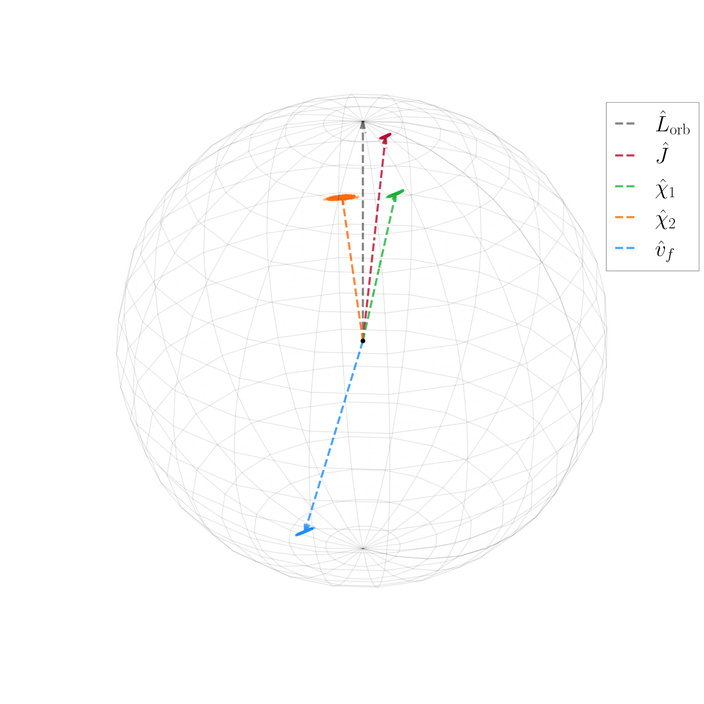
In order to understand the accuracy with which we can infer the remnant properties, we evolve the spins from $f_{\rm low}$ through to the merger, as above, and use the NR calibrated fits of Varma et al. 2019 to estimate the mass $M_{f}$ of the remnant BH, the magnitude of the kick velocity $|v_{f}|$ , and the orientation of the kick velocity $\theta_{v_{f}}$ . For the canonical binary we have focused on here, we find a moderate kick velocity of $|v_{f}|\approx 575\,\rm{km}\,\rm{s}^{-1}$ with an orientation of $\theta_{v_{f}}\approx 165$ deg, as shown in the top right panel of Fig. 6. The top left panel of Fig. 6 highlight the precision to which LISA will be able to resolve the binary geometry in terms of the orientations of $\hat{J},\hat{\chi}_{1},\hat{\chi}_{2}$ , and $\hat{v}_{f}$ . As discussed in Varma et al. 2019, these quantities are defined in an instantaneous frame in which the total orbital angular momentum $\hat{L}_{\rm orb}$ points along $\hat{z}$ at a reference time of $t=-100M$ . Whilst a kick velocity of $v_{f}\approx 575\,\rm{km}\,\rm{s}^{-1}$ is likely to be too small to result in an EM-bright signal Piro et al. 2023, the detection and accurate characterisation of the BH recoil through GW observations alone will allow us to place important constraints on the underlying astrophysical processes. See also the discussion in Gerosa et al. 2015a, which explores differential misalignment and the implications for the kick velocity. As discussed in Gerosa et al. 2015a, kick velocities on the order of $\approx 1500\rm{km}\,\rm{s}^{-1}$ can be produced in highly spinning binaries, with larger kick velocities only being anticipated for comparable mass BHs due to the dynamical alignment of the BH spins. The bottom panel of Fig. 6 shows the posterior distributions on the kick velocity as a function of the tilt of the primary spin at $t=-100M$ for all configurations in the HS series. For the binaries in which the primary spin is essentially orthogonal to $\hat{L}$ , the approaches a maximum on the order of $|v_{f}|\approx 1200\,\rm{km}\,\rm{s}^{-1}$ .

IV Conclusions and Future Work

In this work, we have revisited the Bayesian parameter estimation of MBHBs in LISA using a state-of-the-art inspiral-merger-ringdown waveform model that incorporates both precession and higher multipoles Pratten et al. 2021; Pratten et al. 2020b; García-Quirós et al. 2020. A key focus was to investigate LISA’s capability to accurately constrain the masses and spins of MBHs using the complete GW signal. Given the precision to which LISA can resolve the individual spin magnitudes and orientations, we highlighted how LISA will be able to accurately track the evolution of the BH spins through to the merger. An important consequence is that LISA will be able to accurately predict the magnitude and orientation of the recoil velocity, a key observable in exploring potential EM-bright counterparts to MBH mergers.

In addition to the intrinsic parameters, we also demonstrated that, irrespective of the binary geometry, LISA will be able to constrain the sky location and orientation of the binary to sub-percent level, event out to a redshift of $z\approx 3$ , at least for the subset of binaries considered here. A detailed study exploring a larger population of MBHBs is underway to explore the broader parameter space and the concomitant implications for joint GW-EM analyses.

The detection rate of MBHBs is anticipated to be sensitive to the astrophysical distribution of spin magnitudes and orientations, especially for heavy binaries with $M>10^{7}M_{\odot}$ . Detecting and inferring the properties of these binaries will play a critical role in understanding the astrophysical origin and evolution of MBHs throughout the Universe. This also has important implications in exploring the complex interplay between the MBH population observed by LISA and the stochastic GW background observed by PTAs, for which significant evidence has now been observed Agazie et al. 2023a; Agazie et al. 2023b; Antoniadis et al. 2023a; Antoniadis et al. 2023b; Antoniadis et al. 2023c; Reardon et al. 2023; Xu et al. 2023. In a recent paper, Steinle et al. 2023 demonstrated the implications of observing this PTA background on the anticipated detection rate of MBHBs in LISA. Although Steinle et al. 2023 focused on a systematic suite of non-spinning binaries, the framework can be expanded to incorporate MBHBs with generically oriented spins, as explored here.

Detailed modeling of spin-precession plays a crucial role in resolving parameter degeneracies and enhancing the precision with which we can measure binary parameters Vecchio 2004; Lang and Hughes 2006; Klein et al. 2009; Chatziioannou et al. 2015; Pratten et al. 2020a. It also plays a vital role in exploring MBH formation channels and constraining the astrophysics that drives their mergers. However, an important issue that remains unaddressed here is that of waveform systematics. The stringent accuracy requirements for future waveform models, necessary to reach this level of precision, pose immense challenges for source modelling. Recent developments, such as those in Khalil et al. 2023; Ramos-Buades et al. 2023; Pompili et al. 2023; van de Meent et al. 2023; Yu et al. 2023; Hamilton et al. 2021; Wardell et al. 2023, have shown progress in enhancing the accuracy of the current generation of waveform models. Yet, achieving the accuracy and data analysis demands of LISA still remains a significant endeavor. In future work, we will explore the impact of waveform systematics on our ability to constrain the astrophysics behind MBH mergers. Moreover, we note that the GW signal can be influenced by environmental effects, such as dynamical friction or torquing from angular momentum exchange between accretion discs and the binary Barausse and Rezzolla 2008; Kocsis et al. 2011; Barausse et al. 2014; Speri et al. 2023. Detailed phenomenological modeling of environmental effects opens a promising avenue to discern the astrophysical processes at play in galactic nuclei but could introduce systematic biases into our analysis Zwick et al. 2023.

The results presented here are a first step towards integrating waveform models with precession and higher multipoles into a global fit pipeline. Notably, Littenberg and Cornish 2023 has demonstrated the application of aligned-spin phenomenological waveform models to address the MBHB aspect of the global fit. In our case, we have employed IMRPhenomXPHM to perform Bayesian inference on individual MBHBs. Finally, we note that IMRPhenomXPHM can be effectively combined with the heterodyned likelihood Cornish 2021, even when including precession and higher multipoles Leslie et al. 2021. In forthcoming work, we will build upon the findings presented here to demonstrate how MBHBs can effectively constrain the underlying astrophysical population Pratten et al. In Prep.a and facilitate tests of General Relativity Pratten et al. In Prep.b.

Acknowledgments

We thank Clément Bonnerot and Jean-Baptiste Bayle for useful comments on the manuscript. GP gratefully acknowledges support from a Royal Society University Research Fellowship URF\R1\221500 and RF\ERE\221015. PS and GP acknowledge support from STFC grant ST/V005677/1. HM and AV acknowledge the support of the UK Space Agency Grant No. ST/V002813/1 and ST/X002071/1. AV acknowledges the support of the Royal Society and Wolfson Foundation. Computations were performed on the University of Birmingham’s high performance computing service BlueBEAR and the Bondi HPC Cluster at the Birmingham Institute for Gravitational Wave Astronomy. Parts of this analysis made use of numpy Harris et al. 2020, matplotlib Hunter 2007, scipy Virtanen et al. 2020, numpy Harris et al. 2020, GetDist Lewis 2019, precession Gerosa and Kesden 2016; Gerosa et al. 2023, and dynesty Koposov et al. 2023.

Appendix A Binaries

ID	$m_{1}$	$m_{2}$	$\chi_{1}$	$\chi_{2}$	$\theta_{1}$	$\theta_{2}$	$\phi_{12}$	$z$	$\iota$	$b$	$l$
	$\left[10^{6}M_{\odot}\right]$				$\left[\rm deg\right]$				$\left[\rm deg\right]$
LS1	$1.6$	$0.4$	$0.2$	$0.4$	$21.0$	$31.4$	$34.4$	$3.0$	$10.0$	$17.5$	$114.6$
LS2	$-$	$-$	$-$	$-$	$-$	$-$	$-$	$-$	$42.0$	$-$	$-$
LS3	$-$	$-$	$-$	$-$	$-$	$-$	$-$	$-$	$80.0$	$-$	$-$
LS4	$1.6$	$0.4$	$0.2$	$0.4$	$78.0$	$31.4$	$34.4$	$3.0$	$10.0$	$17.5$	$114.6$
LS5	$-$	$-$	$-$	$-$	$-$	$-$	$-$	$-$	$42.0$	$-$	$-$
LS6	$-$	$-$	$-$	$-$	$-$	$-$	$-$	$-$	$80.0$	$-$	$-$
LS7	$1.6$	$0.4$	$0.2$	$0.4$	$169.0$	$31.4$	$34.4$	$3.0$	$10.0$	$17.5$	$114.6$
LS8	$-$	$-$	$-$	$-$	$-$	$-$	$-$	$-$	$42.0$	$-$	$-$
LS9	$-$	$-$	$-$	$-$	$-$	$-$	$-$	$-$	$80.0$	$-$	$-$

Table 1: Summary table for the low spin (LS) binaries, characterized by

\chi_{1}=0.2

and

\chi_{2}=0.4

. We consider three configurations, corresponding to

\theta_{1}=\{21{\degree},78{\degree},169{\degree}\}

degrees respectively. For each configuration, we consider three inclination angles

\iota=\{10{\degree},42{\degree},80{\degree}\}

to gauge the impact of the binary orientation on our ability to resolve the binary parameters. Here

10

degrees corresponds to a near face-on configuration and

80

degrees to an approximately edge-on configuration. The masses correspond to the source-frame values and a dashed line denotes that the value is equivalent to the row above.

ID	$m_{1}$	$m_{2}$	$\chi_{1}$	$\chi_{2}$	$\theta_{1}$	$\theta_{2}$	$\phi_{12}$	$z$	$\iota$	$b$	$l$
	$\left[10^{6}M_{\odot}\right]$				$\left[\rm deg\right]$				$\left[\rm deg\right]$
HS1	$1.6$	$0.4$	$0.8$	$0.6$	$21.0$	$31.4$	$34.4$	$3.0$	$10.0$	$17.5$	$114.6$
HS2	$-$	$-$	$-$	$-$	$-$	$-$	$-$	$-$	$42.0$	$-$	$-$
HS3	$-$	$-$	$-$	$-$	$-$	$-$	$-$	$-$	$80.0$	$-$	$-$
HS4	$1.6$	$0.4$	$0.8$	$0.6$	$78.0$	$31.4$	$34.4$	$3.0$	$10.0$	$17.5$	$114.6$
HS5	$-$	$-$	$-$	$-$	$-$	$-$	$-$	$-$	$42.0$	$-$	$-$
HS6	$-$	$-$	$-$	$-$	$-$	$-$	$-$	$-$	$80.0$	$-$	$-$
HS7	$1.6$	$0.4$	$0.8$	$0.6$	$169.0$	$31.4$	$34.4$	$3.0$	$10.0$	$17.5$	$114.6$
HS8	$-$	$-$	$-$	$-$	$-$	$-$	$-$	$-$	$42.0$	$-$	$-$
HS9	$-$	$-$	$-$	$-$	$-$	$-$	$-$	$-$	$80.0$	$-$	$-$

Table 2: As in Tab. 1, but now for the high spin (HS) binaries, where

\chi_{1}=0.8

and

\chi_{2}=0.6

Appendix B Summary of Bayesian Inference

Here we list the exact configurations used for the low-spin (LS) and high-spin (HS) binaries. For each set of binaries we fix the sky-location, distance, component masses, spin magnitudes, and spin tilt of the secondary BH. We then systematically vary the spin tilt of the primary BH from an approximately aligned configuration through to an approximately anti-aligned configuration. Spins that are misaligned with the orbital angular momentum give rise to relativistic spin couplings that drive the precession of the orbital plane and the spins themselves Apostolatos et al. 1994; Kidder 1995. By tilting the primary spin we are effectively changing the amount of precession in the binary. In addition to varying the primary spin magnitude, we also explore three binary orientations for each tilt configuration to explore the impact of observing the binary from a near face-on configuration through to a near edge-on configuration. Due to the fact that the binaries undergo multiple precession cycles after entering the observable LISA band, we find that the orientation has little impact on our ability to constrain the BH spins.

Table 3: Summary of the 90% credible intervals on the recovered parameters for all injections considered in this paper. Here HS denotes the high-spin series and LS the low-spin series. The component masses

m_{i}

correspond to the source-frame values,

\chi_{i}

the dimensionless spin magnitudes,

\theta_{i}

the spin-tilt angles, and

\phi_{12}

the difference in the azimuthal spin angles between the two BH spins.

ID	$m_{1}$	$m_{2}$	$\chi_{1}$	$\chi_{2}$	$\theta_{1}$	$\theta_{2}$	$\phi_{12}$	$\theta_{\rm JN}$	$z$	$\sin b$	$l$
	$\left[10^{6}M_{\odot}\right]$	$\left[10^{6}M_{\odot}\right]$	$-$	$-$	$\left[\rm{deg}\right]$	$\left[\rm{deg}\right]$	$\left[\rm{deg}\right]$	$\left[\rm{deg}\right]$	$-$	$-$	$\left[\rm{deg}\right]$
HS1	${1.599}^{+0.001}_{-0.001}$	${0.400}^{+0.0003}_{-0.0003}$	${0.800}^{+0.0003}_{-0.0003}$	${0.600}^{+0.003}_{-0.003}$	${21.0}^{+0.1}_{-0.1}$	${31.5}^{+0.7}_{-0.7}$	${34.5}^{+1.3}_{-1.3}$	${10.00}^{+0.05}_{-0.05}$	${3.002}^{+0.003}_{-0.003}$	${0.300}^{+0.001}_{-0.001}$	${114.59}^{+0.06}_{-0.07}$
HS2	${1.599}^{+0.001}_{-0.001}$	${0.400}^{+0.0004}_{-0.0003}$	${0.800}^{+0.0003}_{-0.0003}$	${0.600}^{+0.003}_{-0.003}$	${21.0}^{+0.1}_{-0.1}$	${31.4}^{+0.7}_{-0.7}$	${34.4}^{+1.5}_{-1.5}$	${42.00}^{+0.06}_{-0.06}$	${3.002}^{+0.003}_{-0.003}$	${0.300}^{+0.001}_{-0.001}$	${114.59}^{+0.03}_{-0.03}$
HS3	${1.599}^{+0.002}_{-0.002}$	${0.400}^{+0.0005}_{-0.0005}$	${0.800}^{+0.0004}_{-0.0003}$	${0.601}^{+0.004}_{-0.004}$	${21.0}^{+0.1}_{-0.1}$	${31.4}^{+0.5}_{-0.5}$	${34.5}^{+1.2}_{-1.2}$	${80.00}^{+0.03}_{-0.03}$	${3.003}^{+0.005}_{-0.005}$	${0.300}^{+0.002}_{-0.002}$	${114.59}^{+0.02}_{-0.02}$
HS4	${1.599}^{+0.002}_{-0.002}$	${0.400}^{+0.0005}_{-0.0006}$	${0.800}^{+0.0012}_{-0.0012}$	${0.600}^{+0.011}_{-0.011}$	${78.0}^{+0.2}_{-0.2}$	${31.4}^{+1.8}_{-1.8}$	${34.2}^{+2.5}_{-2.4}$	${10.00}^{+0.08}_{-0.08}$	${3.002}^{+0.005}_{-0.005}$	${0.300}^{+0.002}_{-0.002}$	${114.59}^{+0.09}_{-0.09}$
HS5	${1.599}^{+0.002}_{-0.002}$	${0.400}^{+0.0006}_{-0.0006}$	${0.800}^{+0.0007}_{-0.0007}$	${0.600}^{+0.012}_{-0.011}$	${78.0}^{+0.2}_{-0.2}$	${31.4}^{+1.2}_{-1.3}$	${34.2}^{+2.4}_{-2.3}$	${42.00}^{+0.04}_{-0.04}$	${3.002}^{+0.006}_{-0.006}$	${0.300}^{+0.002}_{-0.002}$	${114.59}^{+0.03}_{-0.03}$
HS6	${1.599}^{+0.002}_{-0.002}$	${0.400}^{+0.0005}_{-0.0005}$	${0.800}^{+0.0008}_{-0.0008}$	${0.600}^{+0.013}_{-0.013}$	${78.0}^{+0.1}_{-0.1}$	${31.3}^{+1.7}_{-1.7}$	${34.3}^{+3.1}_{-3.3}$	${80.00}^{+0.05}_{-0.05}$	${3.002}^{+0.004}_{-0.004}$	${0.300}^{+0.002}_{-0.002}$	${114.59}^{+0.02}_{-0.02}$
HS7	${1.599}^{+0.005}_{-0.005}$	${0.400}^{+0.0012}_{-0.0012}$	${0.800}^{+0.0040}_{-0.0041}$	${0.599}^{+0.017}_{-0.017}$	${169.0}^{+0.3}_{-0.3}$	${31.5}^{+2.0}_{-1.9}$	${34.6}^{+7.1}_{-7.0}$	${10.00}^{+0.33}_{-0.34}$	${3.002}^{+0.012}_{-0.012}$	${0.300}^{+0.005}_{-0.005}$	${114.59}^{+0.26}_{-0.25}$
HS8	${1.599}^{+0.004}_{-0.004}$	${0.400}^{+0.0011}_{-0.0011}$	${0.800}^{+0.0043}_{-0.0044}$	${0.600}^{+0.009}_{-0.009}$	${169.0}^{+0.3}_{-0.3}$	${31.5}^{+1.6}_{-1.6}$	${34.5}^{+5.5}_{-5.5}$	${42.00}^{+0.11}_{-0.11}$	${3.002}^{+0.011}_{-0.011}$	${0.300}^{+0.005}_{-0.005}$	${114.59}^{+0.07}_{-0.07}$
HS9	${1.599}^{+0.004}_{-0.004}$	${0.400}^{+0.0011}_{-0.0011}$	${0.800}^{+0.0038}_{-0.0037}$	${0.600}^{+0.010}_{-0.010}$	${169.0}^{+0.2}_{-0.2}$	${31.5}^{+1.3}_{-1.3}$	${34.4}^{+4.9}_{-4.9}$	${80.00}^{+0.11}_{-0.11}$	${3.002}^{+0.010}_{-0.010}$	${0.300}^{+0.003}_{-0.003}$	${114.59}^{+0.04}_{-0.04}$
LS1	${1.599}^{+0.005}_{-0.005}$	${0.400}^{+0.001}_{-0.001}$	${0.200}^{+0.004}_{-0.004}$	${0.400}^{+0.014}_{-0.014}$	${21.0}^{+0.5}_{-0.5}$	${31.2}^{+3.8}_{-3.8}$	${34.2}^{+5.6}_{-6.0}$	${10.00}^{+0.08}_{-0.08}$	${3.00}^{+0.01}_{-0.01}$	${0.300}^{+0.003}_{-0.003}$	${114.59}^{+0.18}_{-0.18}$
LS2	${1.599}^{+0.003}_{-0.003}$	${0.400}^{+0.001}_{-0.001}$	${0.200}^{+0.002}_{-0.002}$	${0.400}^{+0.012}_{-0.012}$	${21.0}^{+0.6}_{-0.6}$	${31.7}^{+2.7}_{-2.7}$	${34.3}^{+7.5}_{-8.0}$	${41.99}^{+0.13}_{-0.13}$	${3.00}^{+0.01}_{-0.01}$	${0.300}^{+0.003}_{-0.003}$	${114.59}^{+0.11}_{-0.10}$
LS3	${1.599}^{+0.003}_{-0.003}$	${0.400}^{+0.001}_{-0.001}$	${0.200}^{+0.002}_{-0.002}$	${0.399}^{+0.014}_{-0.014}$	${21.0}^{+0.6}_{-0.6}$	${31.2}^{+2.4}_{-2.3}$	${34.9}^{+6.0}_{-6.1}$	${80.00}^{+0.05}_{-0.05}$	${3.00}^{+0.01}_{-0.01}$	${0.300}^{+0.004}_{-0.004}$	${114.59}^{+0.04}_{-0.04}$
LS4	${1.599}^{+0.004}_{-0.004}$	${0.400}^{+0.001}_{-0.001}$	${0.200}^{+0.002}_{-0.002}$	${0.393}^{+0.024}_{-0.024}$	${77.7}^{+1.1}_{-1.1}$	${30.9}^{+2.8}_{-3.0}$	${35.2}^{+6.6}_{-6.7}$	${10.00}^{+0.07}_{-0.07}$	${3.00}^{+0.01}_{-0.01}$	${0.300}^{+0.003}_{-0.003}$	${114.59}^{+0.18}_{-0.18}$
LS5	${1.599}^{+0.003}_{-0.003}$	${0.400}^{+0.001}_{-0.001}$	${0.200}^{+0.002}_{-0.002}$	${0.398}^{+0.021}_{-0.022}$	${77.8}^{+0.9}_{-0.9}$	${31.3}^{+2.5}_{-2.8}$	${35.7}^{+6.5}_{-6.7}$	${42.00}^{+0.12}_{-0.12}$	${3.00}^{+0.01}_{-0.01}$	${0.300}^{+0.003}_{-0.003}$	${114.59}^{+0.11}_{-0.11}$
LS6	${1.599}^{+0.003}_{-0.003}$	${0.400}^{+0.001}_{-0.001}$	${0.200}^{+0.002}_{-0.002}$	${0.399}^{+0.016}_{-0.016}$	${78.1}^{+0.8}_{-0.8}$	${31.3}^{+2.0}_{-2.1}$	${32.9}^{+6.2}_{-6.6}$	${80.00}^{+0.07}_{-0.07}$	${3.00}^{+0.01}_{-0.01}$	${0.300}^{+0.004}_{-0.004}$	${114.59}^{+0.04}_{-0.04}$
LS7	${1.599}^{+0.007}_{-0.006}$	${0.400}^{+0.001}_{-0.001}$	${0.200}^{+0.006}_{-0.007}$	${0.400}^{+0.020}_{-0.024}$	${169.0}^{+0.5}_{-0.5}$	${31.3}^{+4.8}_{-3.8}$	${34.1}^{+11.9}_{-14.8}$	${10.00}^{+0.17}_{-0.17}$	${3.00}^{+0.01}_{-0.01}$	${0.300}^{+0.004}_{-0.004}$	${114.60}^{+0.22}_{-0.22}$
LS8	${1.599}^{+0.004}_{-0.004}$	${0.400}^{+0.001}_{-0.001}$	${0.200}^{+0.004}_{-0.004}$	${0.401}^{+0.015}_{-0.014}$	${169.0}^{+0.6}_{-0.7}$	${31.3}^{+4.1}_{-3.8}$	${34.8}^{+12.6}_{-12.3}$	${42.00}^{+0.16}_{-0.16}$	${3.00}^{+0.01}_{-0.01}$	${0.300}^{+0.003}_{-0.003}$	${114.59}^{+0.13}_{-0.13}$
LS9	${1.599}^{+0.004}_{-0.004}$	${0.400}^{+0.001}_{-0.001}$	${0.200}^{+0.003}_{-0.003}$	${0.400}^{+0.013}_{-0.013}$	${169.0}^{+0.3}_{-0.3}$	${31.4}^{+2.2}_{-2.1}$	${34.7}^{+10.6}_{-11.1}$	${80.00}^{+0.09}_{-0.09}$	${3.00}^{+0.01}_{-0.01}$	${0.300}^{+0.004}_{-0.004}$	${114.59}^{+0.04}_{-0.04}$

Supplementary Plots

Figure 7 is the low-spin counterpart of Fig. 5, demonstrating that even for low spins, LISA can accurately resolve the magnitudes and orientations of BH spins to a comparable level of accuracy.

Figure 7: As per Fig. 2 but for the low-spin systematic series.

Corner Plots

The complete joint posteriors for our canonical binary configuration, HS2, are shown in Fig. 8.

References

Klein et al. (2016) Antoine Klein et al., “Science with the space-based interferometer eLISA: Supermassive black hole binaries,” Phys. Rev. D 93, 024003 (2016), arXiv:1511.05581 [gr-qc] .
Sesana (2021) Alberto Sesana, “Black Hole Science With the Laser Interferometer Space Antenna,” Front. Astron. Space Sci. 8, 601646 (2021), arXiv:2105.11518 [astro-ph.CO] .
Amaro-Seoane et al. (2023) Pau Amaro-Seoane et al. (LISA), “Astrophysics with the Laser Interferometer Space Antenna,” Living Rev. Rel. 26, 2 (2023), arXiv:2203.06016 [gr-qc] .
Yu and Tremaine (2002) Qing-juan Yu and Scott Tremaine, “Observational constraints on growth of massive black holes,” Mon. Not. Roy. Astron. Soc. 335, 965–976 (2002), arXiv:astro-ph/0203082 .
Tanaka and Haiman (2009) Takamitsu Tanaka and Zoltan Haiman, “The Assembly of Supermassive Black Holes at High Redshifts,” Astrophys. J. 696, 1798–1822 (2009), arXiv:0807.4702 [astro-ph] .
Volonteri (2010) Marta Volonteri, “Formation of Supermassive Black Holes,” Astron. Astrophys. Rev. 18, 279–315 (2010), arXiv:1003.4404 [astro-ph.CO] .
Barausse et al. (2020) Enrico Barausse, Irina Dvorkin, Michael Tremmel, Marta Volonteri, and Matteo Bonetti, “Massive Black Hole Merger Rates: The Effect of Kiloparsec Separation Wandering and Supernova Feedback,” Astrophys. J. 904, 16 (2020), arXiv:2006.03065 [astro-ph.GA] .
Kormendy and Richstone (1995) John Kormendy and Douglas Richstone, “Inward Bound—The Search For Supermassive Black Holes In Galactic Nuclei,” ”Annual Review of Astronomy and Astrophysics” 33, 581 (1995).
Ghez et al. (1998) A. M. Ghez, B. L. Klein, M. Morris, and E. E. Becklin, “High proper motion stars in the vicinity of Sgr A*: Evidence for a supermassive black hole at the center of our galaxy,” Astrophys. J. 509, 678–686 (1998), arXiv:astro-ph/9807210 .
Gebhardt et al. (2000) Karl Gebhardt et al., “A Relationship between Nuclear Black Hole Mass and Galaxy Velocity Dispersion,” ”Astrophysical Journal, Letters” 539, L13–L16 (2000), arXiv:astro-ph/0006289 [astro-ph] .
Ferrarese and Merritt (2000) Laura Ferrarese and David Merritt, “A Fundamental Relation between Supermassive Black Holes and Their Host Galaxies,” ”Astrophysical Journal, Letters” 539, L9–L12 (2000), arXiv:astro-ph/0006053 [astro-ph] .
Schödel et al. (2003) R. Schödel, T. Ott, R. Genzel, A. Eckart, N. Mouawad, and T. Alexander, “Stellar Dynamics in the Central Arcsecond of Our Galaxy,” Astrophys. J. 596, 1015–1034 (2003), arXiv:astro-ph/0306214 [astro-ph] .
Ferrarese and Ford (2005) Laura Ferrarese and Holland Ford, “Supermassive black holes in galactic nuclei: Past, present and future research,” Space Sci. Rev. 116, 523–624 (2005), arXiv:astro-ph/0411247 .
Ghez et al. (2008) A. M. Ghez et al., “Measuring Distance and Properties of the Milky Way’s Central Supermassive Black Hole with Stellar Orbits,” Astrophys. J. 689, 1044–1062 (2008), arXiv:0808.2870 [astro-ph] .
Genzel et al. (2010) Reinhard Genzel, Frank Eisenhauer, and Stefan Gillessen, “The Galactic Center Massive Black Hole and Nuclear Star Cluster,” Rev. Mod. Phys. 82, 3121–3195 (2010), arXiv:1006.0064 [astro-ph.GA] .
Kormendy and Ho (2013) John Kormendy and Luis C. Ho, “Coevolution (Or Not) of Supermassive Black Holes and Host Galaxies,” Ann. Rev. Astron. Astrophys. 51, 511–653 (2013), arXiv:1304.7762 [astro-ph.CO] .
Akiyama et al. (2019) Kazunori Akiyama et al. (Event Horizon Telescope), “First M87 Event Horizon Telescope Results. I. The Shadow of the Supermassive Black Hole,” Astrophys. J. Lett. 875, L1 (2019), arXiv:1906.11238 [astro-ph.GA] .
Bañados et al. (2014) E. Bañados et al., “Discovery of eight z ~ 6 quasars from Pan-STARRS1,” Astron. J. 148, 14 (2014), arXiv:1405.3986 [astro-ph.GA] .
Wu et al. (2015) Xue-Bing Wu et al., “An ultraluminous quasar with a twelve-billion-solar-mass black hole at redshift 6.30,” Nature 518, 512–515 (2015), arXiv:1502.07418 [astro-ph.GA] .
Banados et al. (2018) Eduardo Banados et al., “An 800-million-solar-mass black hole in a significantly neutral Universe at redshift 7.5,” Nature 553, 473–476 (2018), arXiv:1712.01860 [astro-ph.GA] .
Fakhouri et al. (2010) Onsi Fakhouri, Chung-Pei Ma, and Michael Boylan-Kolchin, “The merger rates and mass assembly histories of dark matter haloes in the two Millennium simulations,” Mon. Not. R. Astron. Soc. 406, 2267–2278 (2010), arXiv:1001.2304 [astro-ph.CO] .
Giersz et al. (2015) Mirek Giersz, Nathan Leigh, Arkadiusz Hypki, Nora Lützgendorf, and Abbas Askar, “MOCCA code for star cluster simulations - IV. A new scenario for intermediate mass black hole formation in globular clusters,” Mon. Not. R. Astron. Soc. 454, 3150–3165 (2015), arXiv:1506.05234 [astro-ph.GA] .
O’Leary et al. (2021) Joseph A. O’Leary, Benjamin P. Moster, Thorsten Naab, and Rachel S. Somerville, “EMERGE: empirical predictions of galaxy merger rates since z $\sim$ 6,” Mon. Not. R. Astron. Soc. 501, 3215–3237 (2021), arXiv:2001.02687 [astro-ph.GA] .
Volonteri et al. (2021) Marta Volonteri, Mélanie Habouzit, and Monica Colpi, “The origins of massive black holes,” Nature Reviews Physics 3, 732–743 (2021), arXiv:2110.10175 [astro-ph.GA] .
Madau and Rees (2001) Piero Madau and Martin J. Rees, “Massive black holes as Population III remnants,” Astrophys. J. Lett. 551, L27–L30 (2001), arXiv:astro-ph/0101223 .
Heger et al. (2003) Alexander Heger, C. L. Fryer, S. E. Woosley, N. Langer, and D. H. Hartmann, “How massive single stars end their life,” Astrophys. J. 591, 288–300 (2003), arXiv:astro-ph/0212469 .
Hirano et al. (2014) Shingo Hirano, Takashi Hosokawa, Naoki Yoshida, Hideyuki Umeda, Kazuyuki Omukai, Gen Chiaki, and Harold W. Yorke, “One Hundred First Stars : Protostellar Evolution and the Final Masses,” Astrophys. J. 781, 60–81 (2014), arXiv:1308.4456 [astro-ph.CO] .
Haehnelt and Rees (1993) Martin G. Haehnelt and Martin J. Rees, “The formation of nuclei in newly formed galaxies and the evolution of the quasar population,” Mon. Not. Roy. Astron. Soc. 263, 168–178 (1993).
Loeb and Rasio (1994) Abraham Loeb and Frederic A. Rasio, “Collapse of primordial gas clouds and the formation of quasar black holes,” Astrophys. J. 432, 52 (1994), arXiv:astro-ph/9401026 .
Bromm and Loeb (2003) Volker Bromm and Abraham Loeb, “Formation of the first supermassive black holes,” Astrophys. J. 596, 34–46 (2003), arXiv:astro-ph/0212400 .
Begelman et al. (2006) Mitchell C. Begelman, Marta Volonteri, and Martin J. Rees, “Formation of supermassive black holes by direct collapse in pregalactic halos,” Mon. Not. Roy. Astron. Soc. 370, 289–298 (2006), arXiv:astro-ph/0602363 .
Lodato and Natarajan (2006) Giuseppe Lodato and Priyamvada Natarajan, “Supermassive black hole formation during the assembly of pre-galactic discs,” Mon. Not. R. Astron. Soc. 371, 1813–1823 (2006), arXiv:astro-ph/0606159 [astro-ph] .
Agarwal et al. (2012) Bhaskar Agarwal, Sadegh Khochfar, Jarrett L. Johnson, Eyal Neistein, Claudio Dalla Vecchia, and Mario Livio, “Ubiquitous seeding of supermassive black holes by direct collapse,” Mon. Not. Roy. Astron. Soc. 425, 2854 (2012), arXiv:1205.6464 [astro-ph.CO] .
Volonteri and Rees (2006) Marta Volonteri and M. J. Rees, “Quasars at z=6: The survival of the fittest,” Astrophys. J. 650, 669–678 (2006), arXiv:astro-ph/0607093 .
Ananna et al. (2019) Tonima Tasnim Ananna et al., “The Accretion History of AGNs. I. Supermassive Black Hole Population Synthesis Model,” Astrophys. J. 871, 240 (2019), arXiv:1810.02298 [astro-ph.GA] .
Volonteri et al. (2003) Marta Volonteri, Francesco Haardt, and Piero Madau, “The Assembly and merging history of supermassive black holes in hierarchical models of galaxy formation,” Astrophys. J. 582, 559–573 (2003), arXiv:astro-ph/0207276 .
Hopkins et al. (2006) Philip F. Hopkins et al., “A Unified, merger-driven model for the origin of starbursts, quasars, the cosmic x-ray background, supermassive black holes and galaxy spheroids,” Astrophys. J. Suppl. 163, 1–49 (2006), arXiv:astro-ph/0506398 .
Sesana et al. (2007) Alberto Sesana, Marta Volonteri, and Francesco Haardt, “The imprint of massive black hole formation models on the LISA data stream,” Mon. Not. Roy. Astron. Soc. 377, 1711–1716 (2007), arXiv:astro-ph/0701556 .
Frank and Rees (1976) J. Frank and M. J. Rees, “Effects of massive black holes on dense stellar systems.” Mon. Not. R. Astron. Soc. 176, 633–647 (1976).
Lightman and Shapiro (1977) A. P. Lightman and S. L. Shapiro, “The distribution and consumption rate of stars around a massive, collapsed object.” Astrophys. J. 211, 244–262 (1977).
Quinlan (1996) Gerald D. Quinlan, “The dynamical evolution of massive black hole binaries - I. hardening in a fixed stellar background,” New Astron. 1, 35–56 (1996), arXiv:astro-ph/9601092 .
Begelman et al. (1980) M. C. Begelman, R. D. Blandford, and M. J. Rees, “Massive black hole binaries in active galactic nuclei,” Nature 287, 307–309 (1980).
Gould and Rix (2000) Andrew Gould and Hans-Walter Rix, “Binary black hole mergers from planet-like migrations,” Astrophys. J. Lett. 532, L29 (2000), arXiv:astro-ph/9912111 .
Escala et al. (2005) Andres Escala, Richard B. Larson, Paolo S. Coppi, and Diego Mardones, “The Role of gas in the merging of massive black holes in galactic nuclei. 2. Black hole merging in a clumpy disk,” Astrophys. J. 630, 152–166 (2005), arXiv:astro-ph/0406304 .
Vasiliev et al. (2014) Eugene Vasiliev, Fabio Antonini, and David Merritt, “The final-parsec problem in nonspherical galaxies revisited,” Astrophys. J. 785, 163 (2014), arXiv:1311.1167 [astro-ph.GA] .
Peters and Mathews (1963) P. C. Peters and J. Mathews, “Gravitational radiation from point masses in a Keplerian orbit,” Phys. Rev. 131, 435–439 (1963).
Volonteri et al. (2005) Marta Volonteri, Piero Madau, Eliot Quataert, and Martin J. Rees, “The Distribution and cosmic evolution of massive black hole spins,” Astrophys. J. 620, 69–77 (2005), arXiv:astro-ph/0410342 .
Bogdanovic et al. (2007) Tamara Bogdanovic, Christopher S. Reynolds, and M. Coleman Miller, “Alignment of the spins of supermassive black holes prior to merger,” Astrophys. J. Lett. 661, L147 (2007), arXiv:astro-ph/0703054 .
Berti and Volonteri (2008) Emanuele Berti and Marta Volonteri, “Cosmological black hole spin evolution by mergers and accretion,” Astrophys. J. 684, 822–828 (2008), arXiv:0802.0025 [astro-ph] .
Sesana et al. (2014) A. Sesana, E. Barausse, M. Dotti, and E. M. Rossi, “Linking the spin evolution of massive black holes to galaxy kinematics,” Astrophys. J. 794, 104 (2014), arXiv:1402.7088 [astro-ph.CO] .
Fiacconi et al. (2018) Davide Fiacconi, Debora Sijacki, and J. E. Pringle, “Galactic nuclei evolution with spinning black holes: method and implementation,” Mon. Not. Roy. Astron. Soc. 477, 3807–3835 (2018), arXiv:1712.00023 [astro-ph.GA] .
Reynolds (2019) Christopher S. Reynolds, “Observing black holes spin,” Nature Astron. 3, 41–47 (2019), arXiv:1903.11704 [astro-ph.HE] .
Roedig et al. (2011) C. Roedig, M. Dotti, A. Sesana, J. Cuadra, and M. Colpi, “Limiting eccentricity of subparsec massive black hole binaries surrounded by self-gravitating gas discs,” Mon. Not. R. Astron. Soc. 415, 3033–3041 (2011), arXiv:1104.3868 [astro-ph.CO] .
Farris et al. (2014) Brian D. Farris, Paul Duffell, Andrew I. MacFadyen, and Zoltan Haiman, “Binary Black Hole Accretion From a Circumbinary Disk: Gas Dynamics Inside the Central Cavity,” Astrophys. J. 783, 134 (2014), arXiv:1310.0492 [astro-ph.HE] .
Farris et al. (2015) Brian D. Farris, Paul Duffell, Andrew I. MacFadyen, and Zoltan Haiman, “Binary Black Hole Accretion During Inspiral and Merger,” Mon. Not. Roy. Astron. Soc. 447, L80–L84 (2015), arXiv:1409.5124 [astro-ph.HE] .
Colpi (2014) Monica Colpi, “Massive Binary Black Holes in Galactic Nuclei and Their Path to Coalescence,” Space Sci. Rev. 183, 189–221 (2014), arXiv:1407.3102 [astro-ph.GA] .
Bowen et al. (2018) Dennis B. Bowen, Vassilios Mewes, Manuela Campanelli, Scott C. Noble, Julian H. Krolik, and Miguel Zilhao, “Quasi-Periodic Behavior of Mini-Disks in Binary Black Holes Approaching Merger,” Astrophys. J. Lett. 853, L17 (2018), arXiv:1712.05451 [astro-ph.HE] .
Lense and Thirring (1918) Josef Lense and Hans Thirring, “Ueber den Einfluss der Eigenrotation der Zentralkoerper auf die Bewegung der Planeten und Monde nach der Einsteinschen Gravitationstheorie,” Phys. Z. 19, 156–163 (1918).
Bardeen and Petterson (1975) James M. Bardeen and Jacobus A. Petterson, “The Lense-Thirring Effect and Accretion Disks around Kerr Black Holes,” Astrophys. J. Lett. 195, L65 (1975).
Kumar and Pringle (1985) S. Kumar and J. E. Pringle, “Twisted accretion discs - The Bardeen-Petterson effect,” Mon. Not. R. Astron. Soc. 213, 435–442 (1985).
Scheuer and Feiler (1996) P. A. G. Scheuer and R. Feiler, “The realignment of a black hole misaligned with its accretion disc,” Mon. Not. R. Astron. Soc. 282, 291 (1996).
Natarajan and Pringle (1998) Priyamvada Natarajan and J. E. Pringle, “The Alignment of disk and black hole spins in active galactic nuclei,” Astrophys. J. Lett. 506, L97 (1998), arXiv:astro-ph/9808187 .
Armitage and Natarajan (2002) Philip J. Armitage and Priyamvada Natarajan, “Accretion during the merger of supermassive black holes,” Astrophys. J. Lett. 567, L9–L12 (2002), arXiv:astro-ph/0201318 .
REES (1978) MARTIN J REES, “Relativistic jets and beams in radio galaxies,” Nature 275, 516–517 (1978).
King and Kolb (1999) A. R. King and U. Kolb, “The evolution of black hole mass and angular momentum,” Mon. Not. Roy. Astron. Soc. 305, 654 (1999), arXiv:astro-ph/9901296 .
Gerosa et al. (2015a) Davide Gerosa et al., “Spin alignment and differential accretion in merging black hole binaries,” Mon. Not. Roy. Astron. Soc. 451, 3941–3954 (2015a), arXiv:1503.06807 [astro-ph.GA] .
Coleman Miller and Krolik (2013) M. Coleman Miller and Julian H. Krolik, “Alignment of supermassive black hole binary orbits and spins,” Astrophys. J. 774, 43 (2013), arXiv:1307.6569 [astro-ph.HE] .
Gerosa et al. (2015b) Davide Gerosa et al., “Multi-timescale analysis of phase transitions in precessing black-hole binaries,” Phys. Rev. D 92, 064016 (2015b), arXiv:1506.03492 [gr-qc] .
Steinle and Gerosa (2023) Nathan Steinle and Davide Gerosa, “The Bardeen–Petterson effect, disc breaking, and the spin orientations of supermassive black hole binaries,” Mon. Not. Roy. Astron. Soc. 519, 5031–5042 (2023), arXiv:2211.00044 [astro-ph.HE] .
Doğan et al. (2018) S. Doğan, C. J. Nixon, A. R. King, and J. E. Pringle, “Instability of warped discs,” Mon. Not. Roy. Astron. Soc. 476, 1519–1531 (2018), arXiv:1801.05426 [astro-ph.HE] .
Gerosa et al. (2020) Davide Gerosa, Giovanni Rosotti, and Riccardo Barbieri, “The Bardeen–Petterson effect in accreting supermassive black hole binaries: a systematic approach,” Mon. Not. Roy. Astron. Soc. 496, 3060–3075 (2020), arXiv:2004.02894 [astro-ph.GA] .
Nealon et al. (2021) Rebecca Nealon et al., “The Bardeen–Petterson effect in accreting supermassive black hole binaries: disc breaking and critical obliquity,” Mon. Not. Roy. Astron. Soc. 509, 5608–5621 (2021), arXiv:2111.08065 [astro-ph.HE] .
Vecchio (2004) Alberto Vecchio, “LISA observations of rapidly spinning massive black hole binary systems,” Phys. Rev. D 70, 042001 (2004), arXiv:astro-ph/0304051 .
Lang and Hughes (2006) Ryan N. Lang and Scott A. Hughes, “Measuring coalescing massive binary black holes with gravitational waves: The Impact of spin-induced precession,” Phys. Rev. D 74, 122001 (2006), [Erratum: Phys.Rev.D 75, 089902 (2007), Erratum: Phys.Rev.D 77, 109901 (2008)], arXiv:gr-qc/0608062 .
Lang and Hughes (2008) Ryan N. Lang and Scott A. Hughes, “Localizing coalescing massive black hole binaries with gravitational waves,” Astrophys. J. 677, 1184 (2008), arXiv:0710.3795 [astro-ph] .
Stavridis et al. (2009) Adamantios Stavridis, K. G. Arun, and Clifford M. Will, “Precessing supermassive black hole binaries and dark energy measurements with LISA,” Phys. Rev. D 80, 067501 (2009), arXiv:0907.4686 [gr-qc] .
Lang et al. (2011) Ryan N. Lang, Scott A. Hughes, and Neil J. Cornish, “Measuring parameters of massive black hole binaries with partially aligned spins,” Phys. Rev. D 84, 022002 (2011), arXiv:1101.3591 [gr-qc] .
Tang et al. (2018) Yike Tang, Zoltán Haiman, and Andrew Macfadyen, “The late inspiral of supermassive black hole binaries with circumbinary gas discs in the LISA band,” Mon. Not. Roy. Astron. Soc. 476, 2249–2257 (2018), arXiv:1801.02266 [astro-ph.HE] .
D’Ascoli et al. (2018) Stéphane D’Ascoli et al., “Electromagnetic Emission from Supermassive Binary Black Holes Approaching Merger,” Astrophys. J. 865, 140 (2018), arXiv:1806.05697 [astro-ph.HE] .
Mangiagli et al. (2020) Alberto Mangiagli et al., “Observing the inspiral of coalescing massive black hole binaries with LISA in the era of Multi-Messenger Astrophysics,” Phys. Rev. D 102, 084056 (2020), arXiv:2006.12513 [astro-ph.HE] .
Cutler (1998) Curt Cutler, “Angular resolution of the LISA gravitational wave detector,” Phys. Rev. D 57, 7089–7102 (1998), arXiv:gr-qc/9703068 .
Marsat et al. (2021) Sylvain Marsat, John G. Baker, and Tito Dal Canton, “Exploring the Bayesian parameter estimation of binary black holes with LISA,” Phys. Rev. D 103, 083011 (2021), arXiv:2003.00357 [gr-qc] .
Pratten et al. (2022) Geraint Pratten et al., “On the LISA science performance in observations of short-lived signals from massive black hole binary coalescences,” (2022), arXiv:2212.02572 [gr-qc] .
Apostolatos et al. (1994) Theocharis A. Apostolatos, Curt Cutler, Gerald J. Sussman, and Kip S. Thorne, “Spin induced orbital precession and its modulation of the gravitational wave forms from merging binaries,” Phys. Rev. D 49, 6274–6297 (1994).
Kidder (1995) Lawrence E. Kidder, “Coalescing binary systems of compact objects to postNewtonian 5/2 order. 5. Spin effects,” Phys. Rev. D 52, 821–847 (1995), arXiv:gr-qc/9506022 .
Cutler et al. (1993) Curt Cutler et al., “The Last three minutes: issues in gravitational wave measurements of coalescing compact binaries,” Phys. Rev. Lett. 70, 2984–2987 (1993), arXiv:astro-ph/9208005 .
Chatziioannou et al. (2015) Katerina Chatziioannou, Neil Cornish, Antoine Klein, and Nicolas Yunes, “Spin-Precession: Breaking the Black Hole–Neutron Star Degeneracy,” Astrophys. J. Lett. 798, L17 (2015), arXiv:1402.3581 [gr-qc] .
Pratten et al. (2020a) Geraint Pratten, Patricia Schmidt, Riccardo Buscicchio, and Lucy M. Thomas, “Measuring precession in asymmetric compact binaries,” Phys. Rev. Res. 2, 043096 (2020a), arXiv:2006.16153 [gr-qc] .
Klein et al. (2009) Antoine Klein, Philippe Jetzer, and Mauro Sereno, “Parameter estimation for coalescing massive binary black holes with LISA using the full 2PN gravitational waveform and spin-orbit precession,” Phys. Rev. D 80, 064027 (2009), arXiv:0907.3318 [astro-ph.CO] .
Pratten et al. (2021) Geraint Pratten et al., “Computationally efficient models for the dominant and subdominant harmonic modes of precessing binary black holes,” Phys. Rev. D 103, 104056 (2021), arXiv:2004.06503 [gr-qc] .
García-Quirós et al. (2020) Cecilio García-Quirós et al., “Multimode frequency-domain model for the gravitational wave signal from nonprecessing black-hole binaries,” Phys. Rev. D 102, 064002 (2020), arXiv:2001.10914 [gr-qc] .
Pratten et al. (2020b) Geraint Pratten et al., “Setting the cornerstone for a family of models for gravitational waves from compact binaries: The dominant harmonic for nonprecessing quasicircular black holes,” Phys. Rev. D 102, 064001 (2020b), arXiv:2001.11412 [gr-qc] .
Klein et al. (2022) Antoine Klein et al., “The last three years: multiband gravitational-wave observations of stellar-mass binary black holes,” (2022), arXiv:2204.03423 [astro-ph.HE] .
Toubiana et al. (2020) Alexandre Toubiana, Sylvain Marsat, Stanislav Babak, John Baker, and Tito Dal Canton, “Parameter estimation of stellar-mass black hole binaries with LISA,” Phys. Rev. D 102, 124037 (2020), arXiv:2007.08544 [gr-qc] .
Katz et al. (2022) Michael L. Katz, Jean-Baptiste Bayle, Alvin J. K. Chua, and Michele Vallisneri, “Assessing the data-analysis impact of LISA orbit approximations using a GPU-accelerated response model,” Phys. Rev. D 106, 103001 (2022), arXiv:2204.06633 [gr-qc] .
Digman and Cornish (2022) Matthew C. Digman and Neil J. Cornish, “Parameter Estimation for Stellar-Origin Black Hole Mergers In LISA,” (2022), arXiv:2212.04600 [gr-qc] .
Littenberg and Cornish (2023) Tyson B. Littenberg and Neil J. Cornish, “Prototype global analysis of LISA data with multiple source types,” Phys. Rev. D 107, 063004 (2023), arXiv:2301.03673 [gr-qc] .
Marsat and Baker (2018) Sylvain Marsat and John G. Baker, “Fourier-domain modulations and delays of gravitational-wave signals,” (2018), arXiv:1806.10734 [gr-qc] .
Klein et al. (2014) Antoine Klein, Neil Cornish, and Nicolás Yunes, “Fast Frequency-domain Waveforms for Spin-Precessing Binary Inspirals,” Phys. Rev. D 90, 124029 (2014), arXiv:1408.5158 [gr-qc] .
Klein et al. (2013) Antoine Klein, Neil Cornish, and Nicolás Yunes, “Gravitational waveforms for precessing, quasicircular binaries via multiple scale analysis and uniform asymptotics: The near spin alignment case,” Phys. Rev. D 88, 124015 (2013), arXiv:1305.1932 [gr-qc] .
Prince et al. (2002) Thomas A. Prince, Massimo Tinto, Shane L. Larson, and J. W. Armstrong, “The LISA optimal sensitivity,” Phys. Rev. D 66, 122002 (2002), arXiv:gr-qc/0209039 .
Tinto and Dhurandhar (2005) Massimo Tinto and Sanjeev V. Dhurandhar, “TIME DELAY,” Living Rev. Rel. 8, 4 (2005), arXiv:gr-qc/0409034 .
Buscicchio et al. (2021) Riccardo Buscicchio et al., “Bayesian parameter estimation of stellar-mass black-hole binaries with LISA,” Phys. Rev. D 104, 044065 (2021), arXiv:2106.05259 [astro-ph.HE] .
Rubbo et al. (2004) Louis J. Rubbo, Neil J. Cornish, and Olivier Poujade, “Forward modeling of space borne gravitational wave detectors,” Phys. Rev. D 69, 082003 (2004), arXiv:gr-qc/0311069 .
Skilling (2004) John Skilling, “Nested sampling,” in Aip conference proceedings, Vol. 735 (American Institute of Physics, 2004) pp. 395–405.
Skilling (2006) John Skilling, “Nested sampling for general Bayesian computation,” Bayesian Analysis 1, 833 – 859 (2006).
Speagle (2020) Joshua S. Speagle, “DYNESTY: a dynamic nested sampling package for estimating Bayesian posteriors and evidences,” Mon. Not. R. Astron. Soc. 493, 3132–3158 (2020), arXiv:1904.02180 [astro-ph.IM] .
Koposov et al. (2023) Sergey Koposov et al., “joshspeagle/dynesty: v2.1.2,” (2023).
Cutler and Flanagan (1994) Curt Cutler and Éanna E. Flanagan, “Gravitational waves from merging compact binaries: How accurately can one extract the binary’s parameters from the inspiral waveform\?” Phys. Rev. D 49, 2658–2697 (1994), arXiv:gr-qc/9402014 [gr-qc] .
LISA Science Study Team (2018a) LISA Science Study Team, LISA Science Requirements Document, ESA-L3-EST-SCI-RS-001, Tech. Rep. 1.0 (ESA, 2018).
Team (2018) LISA Science Study Team, LISA Science Requirements Document, Tech. Rep. ESA-L3-EST-SCI-RS-001 (LISA, 2018).
Babak et al. (2017) Stanislav Babak et al., “Science with the space-based interferometer LISA. V: Extreme mass-ratio inspirals,” Phys. Rev. D 95, 103012 (2017), arXiv:1703.09722 [gr-qc] .
Edwards et al. (2020) Matthew C. Edwards et al., “Identifying and Addressing Nonstationary LISA Noise,” Phys. Rev. D 102, 084062 (2020), arXiv:2004.07515 [gr-qc] .
Barker and O’Connell (1970) B. M. Barker and R. F. O’Connell, “Derivation of the equations of motion of a gyroscope from the quantum theory of gravitation,” Phys. Rev. D 2, 1428–1435 (1970).
Barker and O’Connell (1975) B. M. Barker and R. F. O’Connell, “Gravitational Two-Body Problem with Arbitrary Masses, Spins, and Quadrupole Moments,” Phys. Rev. D 12, 329–335 (1975).
Damour (2001) Thibault Damour, “Coalescence of two spinning black holes: an effective one-body approach,” Phys. Rev. D 64, 124013 (2001), arXiv:gr-qc/0103018 .
Racine (2008) Etienne Racine, “Analysis of spin precession in binary black hole systems including quadrupole-monopole interaction,” Phys. Rev. D 78, 044021 (2008), arXiv:0803.1820 [gr-qc] .
Ajith et al. (2011) P. Ajith et al., “Inspiral-merger-ringdown waveforms for black-hole binaries with non-precessing spins,” Phys. Rev. Lett. 106, 241101 (2011), arXiv:0909.2867 [gr-qc] .
Gerosa et al. (2021) Davide Gerosa et al., “A generalized precession parameter $\chi_{\mathrm{p}}$ to interpret gravitational-wave data,” Phys. Rev. D 103, 064067 (2021), arXiv:2011.11948 [gr-qc] .
Abbott et al. (2019) B. P. Abbott et al. (LIGO Scientific, Virgo), “GWTC-1: A Gravitational-Wave Transient Catalog of Compact Binary Mergers Observed by LIGO and Virgo during the First and Second Observing Runs,” Phys. Rev. X 9, 031040 (2019), arXiv:1811.12907 [astro-ph.HE] .
Abbott et al. (2021a) R. Abbott et al. (LIGO Scientific, Virgo), “GWTC-2: Compact Binary Coalescences Observed by LIGO and Virgo During the First Half of the Third Observing Run,” Phys. Rev. X 11, 021053 (2021a), arXiv:2010.14527 [gr-qc] .
Abbott et al. (2021b) R. Abbott et al. (LIGO Scientific, VIRGO, KAGRA), “GWTC-3: Compact Binary Coalescences Observed by LIGO and Virgo During the Second Part of the Third Observing Run,” (2021b), arXiv:2111.03606 [gr-qc] .
Aghanim et al. (2020) N. Aghanim et al. (Planck), “Planck 2018 results. VI. Cosmological parameters,” Astron. Astrophys. 641, A6 (2020), [Erratum: Astron.Astrophys. 652, C4 (2021)], arXiv:1807.06209 [astro-ph.CO] .
Katz et al. (2020) Michael L. Katz, Sylvain Marsat, Alvin J. K. Chua, Stanislav Babak, and Shane L. Larson, “GPU-accelerated massive black hole binary parameter estimation with LISA,” Phys. Rev. D 102, 023033 (2020), arXiv:2005.01827 [gr-qc] .
Schmidt et al. (2015) Patricia Schmidt, Frank Ohme, and Mark Hannam, “Towards models of gravitational waveforms from generic binaries II: Modelling precession effects with a single effective precession parameter,” Phys. Rev. D 91, 024043 (2015), arXiv:1408.1810 [gr-qc] .
Mangiagli et al. (2022) Alberto Mangiagli, Chiara Caprini, Marta Volonteri, Sylvain Marsat, Susanna Vergani, Nicola Tamanini, and Henri Inchauspé, “Massive black hole binaries in LISA: Multimessenger prospects and electromagnetic counterparts,” Phys. Rev. D 106, 103017 (2022), arXiv:2207.10678 [astro-ph.HE] .
Singer and Price (2016) Leo P. Singer and Larry R. Price, “Rapid Bayesian position reconstruction for gravitational-wave transients,” Phys. Rev. D 93, 024013 (2016), arXiv:1508.03634 [gr-qc] .
LISA Science Study Team (2018b) LISA Science Study Team, LISA Science Requirements Document, ESA-L3-EST-SCI-RS-001, Tech. Rep. 1.0 (ESA, 2018).
Combi et al. (2022) Luciano Combi et al., “Minidisk Accretion onto Spinning Black Hole Binaries: Quasi-periodicities and Outflows,” Astrophys. J. 928, 187 (2022), arXiv:2109.01307 [astro-ph.HE] .
Liao et al. (2023) Shihong Liao et al., “Modelling the accretion and feedback of supermassive black hole binaries in gas-rich galaxy mergers,” Mon. Not. Roy. Astron. Soc. 520, 4463 (2023), arXiv:2211.11788 [astro-ph.GA] .
Avara et al. (2023) Mark J. Avara et al., “Accretion onto a Supermassive Black Hole Binary Before Merger,” (2023), arXiv:2305.18538 [astro-ph.HE] .
Dittmann et al. (2023) Alexander J. Dittmann, Geoffrey Ryan, and M. Coleman Miller, “The Decoupling of Binaries from Their Circumbinary Disks,” (2023), arXiv:2303.16204 [astro-ph.HE] .
Gerosa and Kesden (2016) Davide Gerosa and Michael Kesden, “PRECESSION: Dynamics of spinning black-hole binaries with python,” Phys. Rev. D 93, 124066 (2016), arXiv:1605.01067 [astro-ph.HE] .
Gerosa et al. (2023) Davide Gerosa et al., “Efficient multi-timescale dynamics of precessing black-hole binaries,” (2023), arXiv:2304.04801 [gr-qc] .
Kramer (1998) Michael Kramer, “Determination of the geometry of the psr b1913+16 system by geodetic precession,” Astrophys. J. 509, 856 (1998), arXiv:astro-ph/9808127 .
Breton et al. (2008) Rene P. Breton et al., “Relativistic Spin Precession in the Double Pulsar,” Science 321, 104–107 (2008), arXiv:0807.2644 [astro-ph] .
Manchester et al. (2010) R. N. Manchester et al., “Observations and Modelling of Relativistic Spin Precession in PSR J1141-6545,” Astrophys. J. 710, 1694–1709 (2010), arXiv:1001.1483 [astro-ph.GA] .
Perera et al. (2010) B. B. P. Perera et al., “The Evolution of PSR J0737-3039B and a Model for Relativistic Spin Precession,” Astrophys. J. 721, 1193–1205 (2010), arXiv:1008.1097 [astro-ph.GA] .
Fonseca et al. (2014) Emmanuel Fonseca, Ingrid H. Stairs, and Stephen E. Thorsett, “A Comprehensive Study of Relativistic Gravity Using PSR B1534+12,” Astrophys. J. 787, 82 (2014), arXiv:1402.4836 [astro-ph.HE] .
Bonnor and Rotenberg (1961) WB Bonnor and MA Rotenberg, “Transport of momentum by gravitational waves: the linear approximation,” Proceedings of the Royal Society of London. Series A. Mathematical and Physical Sciences 265, 109–116 (1961).
Peres (1962) Asher Peres, “Classical radiation recoil,” Phys. Rev. 128, 2471–2475 (1962).
Bekenstein (1973) Jacob D. Bekenstein, “Gravitational-Radiation Recoil and Runaway Black Holes,” Astrophys. J. 183, 657–664 (1973).
Fitchett (1983) M. J. Fitchett, “The influence of gravitational wave momentum losses on the centre of mass motion of a Newtonian binay system.” Mon. Not. R. Astron. Soc. 203, 1049–1062 (1983).
Gonzalez et al. (2007a) Jose A. Gonzalez et al., “Total recoil: The Maximum kick from nonspinning black-hole binary inspiral,” Phys. Rev. Lett. 98, 091101 (2007a), arXiv:gr-qc/0610154 .
Campanelli et al. (2007) Manuela Campanelli, Carlos O. Lousto, Yosef Zlochower, and David Merritt, “Maximum gravitational recoil,” Phys. Rev. Lett. 98, 231102 (2007), arXiv:gr-qc/0702133 .
Gonzalez et al. (2007b) J. A. Gonzalez et al., “Supermassive recoil velocities for binary black-hole mergers with antialigned spins,” Phys. Rev. Lett. 98, 231101 (2007b), arXiv:gr-qc/0702052 .
Herrmann et al. (2007) Frank Herrmann et al., “Gravitational recoil from spinning binary black hole mergers,” Astrophys. J. 661, 430–436 (2007), arXiv:gr-qc/0701143 .
Lousto and Zlochower (2011) Carlos O. Lousto and Yosef Zlochower, “Hangup Kicks: Still Larger Recoils by Partial Spin/Orbit Alignment of Black-Hole Binaries,” Phys. Rev. Lett. 107, 231102 (2011), arXiv:1108.2009 [gr-qc] .
Varma et al. (2020) Vijay Varma, Maximiliano Isi, and Sylvia Biscoveanu, “Extracting the Gravitational Recoil from Black Hole Merger Signals,” Phys. Rev. Lett. 124, 101104 (2020), arXiv:2002.00296 [gr-qc] .
Varma et al. (2022) Vijay Varma et al., “Evidence of Large Recoil Velocity from a Black Hole Merger Signal,” Phys. Rev. Lett. 128, 191102 (2022), arXiv:2201.01302 [astro-ph.HE] .
Merritt et al. (2004) David Merritt, Milos Milosavljevic, Marc Favata, Scott A. Hughes, and Daniel E. Holz, “Consequences of gravitational radiation recoil,” Astrophys. J. Lett. 607, L9–L12 (2004), arXiv:astro-ph/0402057 .
Komossa and Merritt (2008) S. Komossa and David Merritt, “Gravitational Wave Recoil Oscillations of Black Holes: Implications for Unified Models of Active Galactic Nuclei,” Astrophys. J. Lett. 689, L89 (2008), arXiv:0811.1037 [astro-ph] .
Blecha et al. (2011) Laura Blecha et al., “Recoiling Black Holes in Merging Galaxies: Relationship to AGN Lifetimes, Starbursts, and the M-sigma Relation,” Mon. Not. Roy. Astron. Soc. 412, 2154 (2011), arXiv:1009.4940 [astro-ph.CO] .
Redmount and Rees (1989) I. H. Redmount and M. J. Rees, “Gravitational-radiation rocket effects and galactic structure.” Comments on Astrophysics 14, 165 (1989).
Volonteri et al. (2010) Marta Volonteri, Kayhan Gültekin, and Massimo Dotti, “Gravitational recoil: effects on massive black hole occupation fraction over cosmic time,” Mon. Not. R. Astron. Soc. 404, 2143–2150 (2010), arXiv:1001.1743 [astro-ph.CO] .
Gerosa and Sesana (2015) Davide Gerosa and Alberto Sesana, “Missing black holes in brightest cluster galaxies as evidence for the occurrence of superkicks in nature,” Mon. Not. Roy. Astron. Soc. 446, 38–55 (2015), arXiv:1405.2072 [astro-ph.GA] .
sesana (2007) A. sesana, “Extreme recoils: impact on the detection of gravitational waves from massive black hole binaries,” Mon. Not. Roy. Astron. Soc. 382, 6 (2007), arXiv:0707.4677 [astro-ph] .
Sesana et al. (2009) A. Sesana, M. Volonteri, and F. Haardt, “LISA detection of massive black hole binaries: imprint of seed populations and of exterme recoils,” Class. Quant. Grav. 26, 094033 (2009), arXiv:0810.5554 [astro-ph] .
Milosavljevic and Phinney (2005) Milos Milosavljevic and E. S. Phinney, “The Afterglow of massive black hole coalescence,” Astrophys. J. Lett. 622, L93–L96 (2005), arXiv:astro-ph/0410343 .
O’Neill et al. (2009) Sean M. O’Neill et al., “Reaction of Accretion Disks to Abrupt Mass Loss During Binary Black Hole Merger,” Astrophys. J. 700, 859–871 (2009), arXiv:0812.4874 [astro-ph] .
Schnittman and Krolik (2008) Jeremy D. Schnittman and Julian H. Krolik, “The Infrared Afterglow of Supermassive Black Hole Mergers,” Astrophys. J. 684, 835–844 (2008), arXiv:0802.3556 [astro-ph] .
Lippai et al. (2008) Zoltan Lippai, Zsolt Frei, and Zoltan Haiman, “Prompt Shocks in the Gas Disk Around a Recoiling Supermassive Black Hole Binary,” Astrophys. J. Lett. 676, L5 (2008), arXiv:0801.0739 [astro-ph] .
Megevand et al. (2009) Miguel Megevand et al., “Perturbed disks get shocked: Binary black hole merger effects on accretion disks,” Phys. Rev. D 80, 024012 (2009).
Rossi et al. (2010) Elena M. Rossi et al., “Black hole mergers: the first light,” Mon. Not. R. Astron. Soc. 401, 2021–2035 (2010), arXiv:0910.0002 [astro-ph.HE] .
Komossa (2012) S. Komossa, “Recoiling black holes: electromagnetic signatures, candidates, and astrophysical implications,” Adv. Astron. 2012, 364973 (2012), arXiv:1202.1977 [astro-ph.CO] .
Piro et al. (2023) L. Piro et al., “Chasing Super-Massive Black Hole merging events with $Athena$ and LISA,” Mon. Not. Roy. Astron. Soc. 521, 2577–2592 (2023), arXiv:2211.13759 [astro-ph.HE] .
Varma et al. (2019) Vijay Varma et al., “High-accuracy mass, spin, and recoil predictions of generic black-hole merger remnants,” Phys. Rev. Lett. 122, 011101 (2019), arXiv:1809.09125 [gr-qc] .
Agazie et al. (2023a) Gabriella Agazie et al. (NANOGrav), “The NANOGrav 15 yr Data Set: Evidence for a Gravitational-wave Background,” Astrophys. J. Lett. 951, L8 (2023a), arXiv:2306.16213 [astro-ph.HE] .
Agazie et al. (2023b) Gabriella Agazie et al. (NANOGrav), “The NANOGrav 15-year Data Set: Constraints on Supermassive Black Hole Binaries from the Gravitational Wave Background,” (2023b), arXiv:2306.16220 [astro-ph.HE] .
Antoniadis et al. (2023a) J. Antoniadis et al., “The second data release from the European Pulsar Timing Array I. The dataset and timing analysis,” (2023a), 10.1051/0004-6361/202346841, arXiv:2306.16224 [astro-ph.HE] .
Antoniadis et al. (2023b) J. Antoniadis et al., “The second data release from the European Pulsar Timing Array III. Search for gravitational wave signals,” (2023b), arXiv:2306.16214 [astro-ph.HE] .
Antoniadis et al. (2023c) J. Antoniadis et al., “The second data release from the European Pulsar Timing Array: V. Implications for massive black holes, dark matter and the early Universe,” (2023c), arXiv:2306.16227 [astro-ph.CO] .
Reardon et al. (2023) Daniel J. Reardon et al., “Search for an Isotropic Gravitational-wave Background with the Parkes Pulsar Timing Array,” Astrophys. J. Lett. 951, L6 (2023), arXiv:2306.16215 [astro-ph.HE] .
Xu et al. (2023) Heng Xu et al., “Searching for the Nano-Hertz Stochastic Gravitational Wave Background with the Chinese Pulsar Timing Array Data Release I,” Res. Astron. Astrophys. 23, 075024 (2023), arXiv:2306.16216 [astro-ph.HE] .
Steinle et al. (2023) Nathan Steinle et al., “Implications of pulsar timing array observations for LISA detections of massive black hole binaries,” (2023), arXiv:2305.05955 [astro-ph.HE] .
Khalil et al. (2023) Mohammed Khalil et al., “Theoretical groundwork supporting the precessing-spin two-body dynamics of the effective-one-body waveform models SEOBNRv5,” (2023), arXiv:2303.18143 [gr-qc] .
Ramos-Buades et al. (2023) Antoni Ramos-Buades et al., “SEOBNRv5PHM: Next generation of accurate and efficient multipolar precessing-spin effective-one-body waveforms for binary black holes,” (2023), arXiv:2303.18046 [gr-qc] .
Pompili et al. (2023) Lorenzo Pompili et al., “Laying the foundation of the effective-one-body waveform models SEOBNRv5: improved accuracy and efficiency for spinning non-precessing binary black holes,” (2023), arXiv:2303.18039 [gr-qc] .
van de Meent et al. (2023) Maarten van de Meent et al., “Enhancing the SEOBNRv5 effective-one-body waveform model with second-order gravitational self-force fluxes,” (2023), arXiv:2303.18026 [gr-qc] .
Yu et al. (2023) Hang Yu et al., “IMRPhenomXODE: An Accurate and Efficient Waveform Model for Precessing Binary Black Holes,” (2023), arXiv:2306.08774 [gr-qc] .
Hamilton et al. (2021) Eleanor Hamilton et al., “Model of gravitational waves from precessing black-hole binaries through merger and ringdown,” Phys. Rev. D 104, 124027 (2021), arXiv:2107.08876 [gr-qc] .
Wardell et al. (2023) Barry Wardell et al., “Gravitational Waveforms for Compact Binaries from Second-Order Self-Force Theory,” Phys. Rev. Lett. 130, 241402 (2023), arXiv:2112.12265 [gr-qc] .
Barausse and Rezzolla (2008) Enrico Barausse and Luciano Rezzolla, “The Influence of the hydrodynamic drag from an accretion torus on extreme mass-ratio inspirals,” Phys. Rev. D 77, 104027 (2008), arXiv:0711.4558 [gr-qc] .
Kocsis et al. (2011) Bence Kocsis, Nicolas Yunes, and Abraham Loeb, “Observable Signatures of EMRI Black Hole Binaries Embedded in Thin Accretion Disks,” Phys. Rev. D 84, 024032 (2011), arXiv:1104.2322 [astro-ph.GA] .
Barausse et al. (2014) Enrico Barausse, Vitor Cardoso, and Paolo Pani, “Can environmental effects spoil precision gravitational-wave astrophysics?” Phys. Rev. D 89, 104059 (2014), arXiv:1404.7149 [gr-qc] .
Speri et al. (2023) Lorenzo Speri et al., “Probing Accretion Physics with Gravitational Waves,” Phys. Rev. X 13, 021035 (2023), arXiv:2207.10086 [gr-qc] .
Zwick et al. (2023) Lorenz Zwick, Pedro R. Capelo, and Lucio Mayer, “Priorities in gravitational waveforms for future space-borne detectors: vacuum accuracy or environment?” Mon. Not. Roy. Astron. Soc. 521, 4645–4651 (2023), arXiv:2209.04060 [gr-qc] .
Cornish (2021) Neil J. Cornish, “Heterodyned likelihood for rapid gravitational wave parameter inference,” Phys. Rev. D 104, 104054 (2021), arXiv:2109.02728 [gr-qc] .
Leslie et al. (2021) Nathaniel Leslie, Liang Dai, and Geraint Pratten, “Mode-by-mode relative binning: Fast likelihood estimation for gravitational waveforms with spin-orbit precession and multiple harmonics,” Phys. Rev. D 104, 123030 (2021), arXiv:2109.09872 [astro-ph.IM] .
Pratten et al. (In Prep.a) Geraint Pratten et al., (In Prep.a).
Pratten et al. (In Prep.b) Geraint Pratten et al., (In Prep.b).
Harris et al. (2020) Charles R. Harris et al., “Array programming with NumPy,” Nature 585, 357–362 (2020).
Hunter (2007) J. D. Hunter, “Matplotlib: A 2d graphics environment,” Computing in Science & Engineering 9, 90–95 (2007).
Virtanen et al. (2020) Pauli Virtanen et al., “SciPy 1.0: Fundamental Algorithms for Scientific Computing in Python,” Nature Methods 17, 261–272 (2020).
Lewis (2019) Antony Lewis, “GetDist: a Python package for analysing Monte Carlo samples,” (2019), arXiv:1910.13970 [astro-ph.IM] .