Multi-representations Space Separation based Graph-level Anomaly-aware DetectionConference: 35th International Conference on Scientific and Statistical Database Management; July 10–12, 2023; Los Angeles, CA, USA35th International Conference on Scientific and Statistical Database Management (SSDBM 2023), July 10–12, 2023, Los Angeles, CA, USAPrice: 15.00DOI: 10.1145/3603719.3603739ISBN: 979-8-4007-0746-9/23/07CCS: Security and privacy Intrusion/anomaly detection and malware mitigationCCS: Computing methodologies Neural networks
Abstract.
Graph structure patterns are widely used to model different area data recently. How to detect anomalous graph information on these graph data has become a popular research problem. The objective of this research is centered on the particular issue that how to detect abnormal graphs within a graph set. The previous works have observed that abnormal graphs mainly show node-level and graph-level anomalies, but these methods equally treat two anomaly forms above in the evaluation of abnormal graphs, which is contrary to the fact that different types of abnormal graph data have different degrees in terms of node-level and graph-level anomalies. Furthermore, abnormal graphs that have subtle differences from normal graphs are easily escaped detection by the existing methods. Thus, we propose a multi-representations space separation based graph-level anomaly-aware detection framework in this paper. To consider the different importance of node-level and graph-level anomalies, we design an anomaly-aware module to learn the specific weight between them in the abnormal graph evaluation process. In addition, we learn strictly separate normal and abnormal graph representation spaces by four types of weighted graph representations against each other including anchor normal graphs, anchor abnormal graphs, training normal graphs, and training abnormal graphs. Based on the distance error between the graph representations of the test graph and both normal and abnormal graph representation spaces, we can accurately determine whether the test graph is anomalous. Our approach has been extensively evaluated against baseline methods using ten public graph datasets, and the results demonstrate its effectiveness. The code for our method is publicly available on https://github.com/whb605/MssGAD.git
Keywords:
graph anomaly detection, graph neural networks, graph representation learning1. Introduction
The application of graph structure pattern (Zhang et al. 2018b; Luo et al. 2020) is widely exploited in various scenarios. For example, people are associated with performing various social activities on social networks, and every user is affiliated with rich profile information. So users are as attributed nodes and relationships of users are as edges when social networks are treated as graphs. As the population of various graphs, graph anomaly detection application (Ma et al. 2021; Akoglu et al. 2015) gets increasing attention in recent years. Graph anomaly detection primarily aims to pinpoint uncommon nodes or graphs that exhibit significant deviations from the majority of other nodes or graphs within a given set of graph data. Thus, in this work, we concentrate on detecting abnormal graphs within a graph set, i.e., graph-level anomaly detection(GLAD), which is also especially significant in real-life applications. As an illustration, GLAD can be utilized to identify unusual molecules in extensive collections of molecules that are depicted as molecular graphs, where atoms are illustrated as nodes and bonds are represented as edges. This is because abnormal molecules have distinct structures and features in their corresponding graphs compared to other molecules. Similarly, compared with traditional financial fraud detection technology (Dou et al. 2020; Zhang et al. 2022), GLAD can not only intuitively present the complex topology implied in the data, but also integrate the correlation between data objects into the fraud identification task, making it easier to identify the fraud that is hard to find. In conclusion, GLAD is more worth developing to improve the performance of anomalous graph detection.
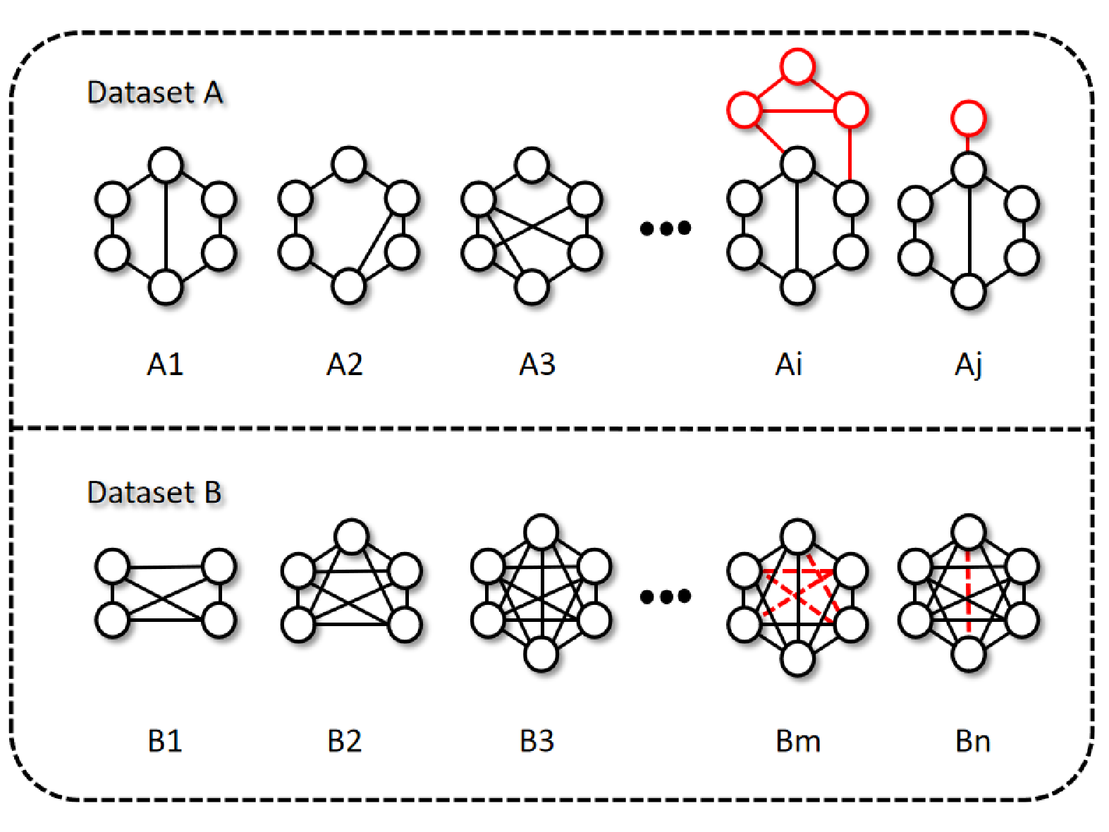
In recent years, GLAD has gradually received attention and some methods have achieved good performance. Several studies have shown that GLAD can achieve promising results by utilizing off-the-shelf methods like one-class support vector machine (OCSVM)(Schölkopf et al. 1999) and isolation forest (iForest)(Liu et al. 2008). However, the efficacy of these detection methods is restricted, because these measures are not good at extracting effective node-level and graph-level representations on complex graph data and the evaluation strategy is shallow. Due to the remarkable development of deep learning, some commonly used graph deep learning methods (Wu et al. 2020) are migrated to GLAD and have shown excellent performance. such as (Chen et al. 2017; Hawkins et al. 2002; Pang et al. 2018; Pang et al. 2019; Perera and Patel 2019). These approaches initially investigate the observation that abnormal graphs consistently manifest anomalies at both the node and graph levels. Subsequently, these methods employ encoders based on graph neural networks (GNNs) (Kipf and Welling 2017; Veličković et al. 2017; Hamilton et al. 2017) to learn node-level and graph-level representations of normal graphs, and then determine the normality of a graph by computing node-level and graph-level reconstruction losses. However, these methods equally treat node-level anomaly and graph-level anomaly in the evaluation process of abnormal graphs, while the manifestation of anomalous graphs may vary in different graph sets. In other words, every type of graph data shows different degrees of node-level and graph-level anomalies. For instance, anomalous molecule graphs, differ from other normal molecule graphs in terms of the global structure, i.e., graph-level anomaly. But anomalous graphs are always node attribute anomalies or user connectivity anomalies in social network graphs, i.e., node-level anomaly. In addition, normal and abnormal graphs may be similar in some graph sets. If we only rely on the popular anomaly evaluation way based on graph representation reconstruction error, these abnormal graphs with subtle differences are difficult to be identified. Figure 1 illustrates a specific example. Thus, existing methods have not taken the above problems into account very well, and as a result, their performance in graph anomaly detection is also affected.
In this paper, a new approach for detecting the graph-level anomaly, namely Multi-representations Space Separation based Graph-level Anomaly-aware Detection(MssGAD), is introduced to address the aforementioned challenges. In order to more effectively account for the varying significance of node-level and graph-level anomalies across different sets of graphs, we devise an anomaly-aware approach that dynamically adjusts the weighting of node-level and graph-level anomalies in the overall detection of graph anomalies. Furthermore, we learn a separate multi-representations space to differentiate normal graph representation space and abnormal graph representation space. Specifically, we select a certain number of graph samples from normal and anomalous graphs of the training set as anchor normal graphs and anchor abnormal graphs. Then, we train the proposed framework to make normal graphs closer to the anchor normal graph and anomalous graphs closer to the anchor anomalous graph under the weighted graph representation guidance. Thus, we can get contractible and separate anchor normal graph representation space and anchor abnormal graph representation space. Finally, we judge graph is normal or not by comparing the distances between it and the two kinds of graph representation spaces above. Therefore, the primary achievements of this research can be highlighted as:
-
We present a framework for detecting the graph-level anomaly through the use of the anomaly-aware strategy. For different graph sets, we dynamically adjust the weight of node-level anomaly and graph-level anomaly in the customized loss function optimization, to better adapt to different graph sets.
-
We propose a multi-representation space separation method, which can gradually increase the distance between anchor normal graph representation space and anchor abnormal graph representation space during the training process. And we transfer the GLAD problem to the task of computing and comparing the distances between test graphs and two anchor graph representation spaces.
-
We propose a new GLAD framework, namely MssGAD, which can effectively finish the task of graph-level anomaly detection. It also shows remarkable robustness to different datasets and it is not sensitive to the abnormal graph label in the collection.
The remaining sections of this paper are structured as follows: Section 2 provides an overview of related research. Section 3 elaborates on the problem definition of graph-level anomaly detection. Section 4 presents a comprehensive description of the implementation process and details of our framework. Section 5 showcases our method’s experimental setup and results on various graph sets and compares our approach with some baseline methods. Finally, Section 6 provides concluding remarks.
2. Related Work
With the continuous attention of researchers, graph neural networks have been developed significantly and many graph anomaly detection methods based on them have been proposed, and in this section, we present the related work from the above two aspects.
2.1. Graph Neural Networks
GNNs (Kipf and Welling 2017; Veličković et al. 2017; Wu et al. 2020) are a type of neural network that can operate directly on graph-structured data. Conventional neural networks can handle vector or sequence information, and GNNs can learn and reason about relationships between objects represented as nodes in a graph and edges connecting them. GNNs have demonstrated significant promise in numerous tasks, including node classification (Gao et al. 2018; Rong et al. 2019; Wang et al. 2020), link prediction (Zhang and Chen 2018; Gou and Wu 2022; Chen et al. 2022a), and graph clustering (Zhang et al. 2018a; Errica et al. 2019; Lee et al. 2018). A major benefit of GNNs is their capacity to grasp not only the local properties but also the global information of a graph, allowing them to make accurate predictions based on the structural characteristics of the graph.
There are various kinds of GNNs, including graph convolutional networks (GCNs) (He et al. 2020; Wu et al. 2019; Park et al. 2022; Liao et al. 2022), graph attention networks (GATs) (Veličković et al. 2017; Wang et al. 2019), and graph recurrent neural networks (GRNNs) (Hajiramezanali et al. 2019; Geng et al. 2022), each with its unique architecture and approach to graph learning. As interest in graph analysis continues to grow and graph-structured data becomes increasingly available, the use of GNNs is now crucial for data mining and many artificial intelligence topics will also utilize GNNs. We make use of GCNs in this paper to obtain node-level and graph-level representations of graphs, which enable us to identify graph anomalies from both local and global standpoints.
2.2. Graph Anomaly Detection
Graph anomaly detection involves identifying unusual patterns or behaviors in a dataset that is represented as a graph. This technique can be categorized into two types: graph-level anomaly detection (GLAD) and node-level anomaly detection (NLAD). Unlike traditional anomaly detection methods that operate on tabular or vector data, GLAD aims to identify the graphs which have unusual or unexpected patterns in a graph set. NLAD refers to identifying the nodes which are significantly different from others in a single graph.
Many GNNs-based graph anomaly detection approaches have been used and reached great performance. For instance, some NLAD methods (Tang et al. 2022; Le Bars and Kalogeratos 2019; Jingcan et al. 2022) concentrate on detecting abnormal nodes or edges within a vast graph. In addition, other NLAD methods (Chen et al. 2022b; Jin et al. 2021) consider building contrast instances to extract abnormal relationships of nodes. Recently, some GLAD methods such as (Ma et al. 2022; Luo et al. 2022; Zhao and Akoglu 2021) focus on graph-level anomaly detection, and their performance is better than traditional shallow approaches (Liu et al. 2008; Breunig et al. 2000) on different graph sets. GLocalKD (Ma et al. 2022) is one example of a method that utilized graph representation distillation to obtain errors in node-level and graph-level representations, which are subsequently employed for the detection of anomalous graphs. OCGTL (Qiu et al. 2022) used advanced neural transformation learning to improve one-class classification performance in GLAD tasks. Other methods based on graph out-of-distribution detection are proposed, such as GOOD-D (Liu et al. 2023) and GraphDE (Li et al. 2022).
But it should be noted that the manifestation of graph anomalies in different graph sets is not always consistent. Existing GLAD methods do not deal well with this problem, therefore, these methods failed to achieve good generalization performance. For example, the difference between anomalous and normal graphs in some datasets may specifically be more reflected at the node level, while in other datasets it is more reflected at the graph level. In response, we propose an anomaly-aware module that leverages dynamic factors to more accurately adjust the weight of graph-level and node-level anomalies in the overall detection of anomalies. And for the issue that anomalous patterns in some datasets are more subtle and difficult to grasp than others, we learn separate anchor normal graph representation space and anchor abnormal graph representation space to detect anomalous graphs more precisely.
3. Preliminaries
3.1. Definition
A graph set is represented as , where z indicates the number of graphs in the dataset. And a single graph is denoted as , where denotes the set of nodes, denotes the set of edges and denotes the set of node attribute in the graph respectively. If the graph is attributed, the feature vector of node , denoted by , is generated by the node’s attributes or labels. If the graph is not attributed, then represents the degree of node . Moreover, is an adjacency matrix that denotes the topology of graph , is assigned 1 when the edge between and exists, and by contrast, 0 when not.
- •
Node-level anomaly means that a graph has unusual node attributes or labels and anomalous edges between nodes compared with nodes of normal graphs. We evaluate such anomalies by node-level representations. The node-level representations is the fusion feature distilled from node neighbors’ attributes and connection status between nodes which is denoted by .
- •
Graph-level anomaly indicates that there is an inconsistency in the overall structure of a particular graph compared to normal graphs. We capture this difference through graph-level representations. The graph-level representations concentrate on the more comprehensive information of the whole graph which is denoted by . In order to derive the graph-level representations, we apply a max-pooling operation to the node-level representations of each dimension for all nodes in the graph, and the specific formula is shown below:
(1) where the dimension of the node-level representations is d.

3.2. Problem Statement
Given a graph set , where denotes an unlabeled graph that may be normal or abnormal, we aim to train a model which can proficiently identify anomalous graphs that demonstrate substantial deviations from the majority of normal graphs in both node-level and graph-level anomalies.
4. Methods
We introduce a framework for identifying graph-level anomalies in this section, which merges node-level and graph-level representations of graphs. The overall structure of the MssGAD framework we propose is illustrated in Figure 2. As a point of emphasis, we introduce the anomaly-aware module and the multi-representations space separation in detail and explain how they assist the model to identify more salient features. Then we describe the critical way to compute the score for anomaly detection.
| Datasets | AIDS | DHFR | MUTAG | PTC-FM | HSE | MMP | P53 | PPAR | ENZYMES | PROTEINS |
|---|---|---|---|---|---|---|---|---|---|---|
| GRAPHS | 2000 | 756 | 188 | 349 | 8150 | 7320 | 8634 | 8184 | 600 | 1113 |
| AVG-NODES | 15.69 | 42.43 | 17.93 | 14.11 | 16.72 | 17.49 | 17.79 | 17.23 | 32.63 | 39.06 |
| AVG-EDGES | 16.2 | 44.54 | 19.79 | 14.48 | 17.04 | 17.83 | 18.19 | 17.55 | 62.14 | 72.82 |
| Datasets | FGSD-IF | FGSD-LOF | FGSD-OCSVM | GOOD-D | OCGTL | MssGAD | ||||||
| A=0 | A=1 | A=0 | A=1 | A=0 | A=1 | A=0 | A=1 | A=0 | A=1 | A=0 | A=1 | |
| AIDS | 99.35±0.75 | 0.65±0.75 | 87.92±3.45 | 12.08±3.45 | 83.47±4.89 | 16.50±4.89 | 92.62±2.19 | 14.56±7.39 | 94.89±3.74 | 98.90±1.13 | 99.61±0.76 | 98.87±0.45 |
| DHFR | 51.51±4.09 | 48.49±4.09 | 49.05±5.97 | 50.95±5.97 | 55.05±6.37 | 44.95±6.37 | 62.82±2.98 | 61.35±4.73 | 71.77±8.78 | 50.15±6.22 | 72.24±2.05 | 72.27±2.87 |
| MUTAG | 78.98±8.67 | 21.02±8.67 | 74.45±5.94 | 25.55±5.94 | 57.70±5.71 | 42.30±5.71 | 79.41±2.45 | 18.64±8.66 | 86.41±9.34 | 82.05±9.56 | 90.07±3.42 | 89.18±4.74 |
| PTC-FM | 40.86±5.48 | 59.14±5.48 | 42.88±4.83 | 57.12±4.83 | 50.38±7.88 | 49.62±7.88 | 54.85±5.76 | 51.37±5.45 | 60.52±5.06 | 46.56±3.97 | 61.58±3.59 | 62.19±5.00 |
| HSE | 39.26±2.19 | 60.74±2.19 | 42.86±3.28 | 57.14±3.28 | 42.13±2.78 | 57.87±2.78 | 66.86±3.05 | 55.98±3.37 | 64.98±4.34 | 64.57±4.06 | 55.76±7.26 | 52.87±6.85 |
| MMP | 67.97±1.08 | 32.03±1.08 | 57.71±1.78 | 42.29±1.78 | 51.90±2.04 | 48.10±2.04 | 70.14±2.09 | 52.85±3.44 | 61.01±1.34 | 80.53±1.27 | 68.07±0.75 | 68.05±0.81 |
| P53 | 66.83±2.35 | 33.17±2.35 | 57.26±1.58 | 42.74±1.58 | 48.64±3.03 | 51.36±3.03 | 62.88±2.29 | 58.73±2.23 | 61.92±5.25 | 75.98±4.34 | 62.19±8.78 | 60.59±5.61 |
| PPAR | 34.83±3.10 | 65.17±3.10 | 47.14±4.96 | 52.86±4.96 | 50.13±5.27 | 49.87±5.27 | 66.61±1.55 | 55.01±4.07 | 61.07±4.10 | 70.36±6.58 | 61.04±7.04 | 65.76±3.94 |
| ENZYMES | 47.82±5.27 | 48.47±6.96 | 38.68±6.03 | 46.36±5.92 | 42.72±5.40 | 55.04±5.31 | 63.16±4.58 | 54.79±5.81 | 65.84±12.50 | 64.44±6.48 | 65.90±5.68 | 57.42±6.41 |
| PROTEINS | 75.30±2.21 | 24.68±2.21 | 58.29±3.74 | 41.71±3.74 | 31.81±0.83 | 68.19±0.83 | 72.20±4.00 | 72.32±3.32 | 59.34±1.27 | 64.78±2.96 | 77.24±3.04 | 76.63±3.41 |
4.1. Anomaly-aware Module
The key intuition of the anomaly-aware module is that the model is utilized to detect graph-level anomalies. The distinction between normal and abnormal graphs can be more specifically attributed to either the node level or the graph level. To account for this, we present an anomaly-aware module that assesses whether the anomalous pattern is mainly manifested in the node-level representations or the graph-level representations.
First, we divided the graph set into two sets and , contains normal graphs, and contains abnormal graphs. And we randomly extract a certain ratio of samples from and respectively denoted by and . Under ideal conditions, the specific proportion of sampling should be determined by the distributions of graphs in the embedding space. However, the distributions are unknown. Therefore, after experiments with various parameters, we finally determine the ratio of sampling as follows:
| (2) |
where represents the number of anchor graphs, while corresponds to the total number of graphs within the set that have the same label. These samples are anchor graphs for the model during training.
Subsequently, we utilize a graph neural network model to acquire both node-level and graph-level representations. We use the original graph-level and node-level representations of , , and to calculate four significant distances denoted by :
| (3) |
| (4) |
| (5) |
| (6) |
where denotes the node representations of graphs in , denotes the node representations of graphs in and denotes the node representations of graphs in . Similarly, the graph-level representations of the graphs in the three aforementioned graph sets are respectively referred to as , , and . The function denotes the feature extraction process of node-level representations which can be common functions such as and , or more complex functions. In experiments, we use as . By combining both node-level representations and graph-level representations, the first two distances determine the dissimilarities between normal graphs and anchor normal graphs, while the latter two are relevant to normal graphs and anchor abnormal graphs.
We refer to the Euclidean distance between and as the node-level representation difference and the Euclidean distance between and as the graph-level representation difference. These two distances assist us to evaluate which level of representation varies more significantly so that we can pay more attention to it during training. To quantify how much we focus on two levels of representations, we introduce two changeable weight factors and . Specifically, if the node-level representation difference is more than twice as large as the graph-level representation difference, is empirically set to 0 while is set to 1, by which we emphasize the node-level representations when calculating the multi-representations space distances. On the contrary, if the graph-level representation difference is more than twice as large as the node-level representation difference, to utilize the graph-level representations, we set to 1 and to 0. In other cases, and are equally set to 0.5 to fuse both of them. By using the anomaly-aware module to dynamically determine the weight factors, our model is able to adapt to different patterns of graph anomaly.
4.2. Multi-representations Space Separation
The motivation is the distribution of feature vectors in the embedding space can be very complex. The distribution of some anomalous graphs may be very close to that of normal graphs, making it difficult to discern subtle differences between them. Therefore the model may be misled and only achieve sub-optimal effects. To tackle this challenge, we utilize the extracted anchor graphs , and in the anomaly-aware module to guide the normal and abnormal graphs to be separated.
We map the above four graph sets to the multi-representation space by fusing the graph-level representations and node-level representations in a weighted way. The specific graph representation space distances can be given as:
| (7) |
| (8) |
| (9) |
| (10) |
| (11) |
We can denote the graph representation space distance between normal graphs and anchor normal graphs by , normal graphs and anchor abnormal graphs by , anchor normal graphs and anchor abnormal graphs by . Likewise, we can obtain the graph representation space distance between abnormal graphs and anchor normal graphs denoted by as well as which between abnormal graphs and anchor abnormal graphs denoted by .
During training, we can present the training loss function as:
| (12) |
| (13) |
In each epoch, we train the graph neural network model with normal graphs by minimizing the , and then with abnormal graphs by the . So that the model can learn every graph in the training set. And we drive the anchor normal graphs and the anchor abnormal graphs apart by the constraint of in the loss function and then make normal graphs close to anchor normal graphs under the action of while far away from anchor abnormal graphs due to . Symmetrically, the abnormal graphs will approach the anchor abnormal graphs because of and escape from the anchor normal graphs as a result of . Generally, the multi-representations space distance between normal graphs and abnormal graphs will vary to be bigger. So it is less difficult for the model to learn their feature distinctions. And during inference, the performance of the anomaly score based on multi-representations space distances will be better as well.
4.3. Graph Anomaly Evaluation
The graph anomaly evaluation is mainly based on the multi-represen-tations space distance between the unlabeled graph set and anchor normal graphs as well as the one between the unlabeled graph set and anchor abnormal graphs. We don’t take the whole normal graphs set or the abnormal graphs set into account. Because our anomaly score is dependent on the distance, we hope to select the graphs with more typical features, namely the anchor graphs, to reduce the impact of the singular graphs and improve the precision.
Specifically, to detect abnormal graphs with the trained model, we can calculate two vital graph representation space distances of a given graph . denotes the graph representation space distance between and , and denotes the graph representation space distance between and as follows:
| (14) |
| (15) |
| (16) |
If belongs to the normal graphs set, will be greater than a certain threshold value, on the contrary, being smaller than the threshold value indicates is more likely to be anomalous. Empirically and ideally, we use 0 as the threshold value. Finally, the algorithm 1 shows the detailed training process of MssGAD.
Calculate the count of anchor normal graphs as and the count of anchor abnormal graphs as by Eq.(2);
Randomly draw an anchor normal graph set with a size of from and an anchor abnormal graph set with a size of from ;
Calculate , , , by Eq.(3), Eq.(4), Eq.(5), Eq.(6);
Determine the value of and by , , , ;
Use graph set as training set; 1
for to do 3
Calculate on the normal graph set by Eq.(7), Eq.(8), Eq.(9);
Update by minimizing shown in Eq.(12); end for 4
for to v do 5
Calculate on the normal graph set by Eq.(9), Eq.(10), Eq.(11);
Update by minimizing shown in Eq.(13); end for 6
Distill and from by Eq.(1);
Calculate on the unlabeled graph sample by Eq.(14), Eq.(15);
Calculate on unlabeled graph sample by Eq.(16);
8
5. Experiment
In this section, we present an evaluation of the MssGAD model on diverse publicly available datasets from various domains and compare its performance with several other anomaly detection methods proposed in recent years. Based on this, we then design and conduct several comparative experiments and try to interpret and validate the effectiveness of our model design through the results of these experiments.
5.1. Datasets
For the selection of datasets, ten different datasets are selected from multiple fields such as toxic substances, molecular compounds, macromolecular proteins, etc. HSE, MMP, p53, and PPAR are datasets established to predict the properties and effects of compounds according to their chemical structures, which contain thousands of potentially harmful chemicals. AIDS is an antiviral screening dataset used for NCI / NIH development and treatment programs. DHFR is a dihydrofolate reductase inhibitors dataset that contains structural information for 325 compounds. For each compound, 228 molecular descriptors have been calculated. PTC-FM contains compounds that are carcinogenic markers for rodents. The ENZYMES and PROTEINS datasets are composed of protein structures, where graphs correspond to individual proteins and nodes correspond to secondary structure elements. Two nodes are connected by an edge if they are adjacent in either the amino acid sequence or 3D space. Table 1 presents the specifics of these datasets. These datasets are not identical in structure because they belong to different domains, some of them contain node features and others do not, therefore we use the degrees of the nodes to replace node features when they do not exist. In addition, we will take one class of graphs as anomalous graphs, while the graphs of the other categories will be treated as normal graphs during experiments.
5.2. Baselines
For the choice of comparing methods, we select three more traditional methods: FGSD-IF (Liu et al. 2008), FGSD-LOF (Breunig et al. 2000), and FGSD-OCSVM (Schölkopf et al. 1999), which are commonly based on the Family of Graph Spectral Distances (FGSD) (Verma and Zhang 2017). FGSD is a method to embed node pairwise distances and obtain the graph feature representations which exhibits certain stability and uniqueness, while isolation forest (IF), local outlier factor (LOF), and one-class support vector machine (OCSVM) are three classical classifiers combined with FGSD. Furthermore, GOOD-D (Liu et al. 2023) is selected because it is a contrastive learning-based unsupervised graph anomaly detection approach that has been recently introduced. In addition, OCGTL (Qiu et al. 2022) is a graph-level anomaly detection method that incorporates concepts from transformation learning and self-supervised learning, and has recently set a new standard in this area. To make MssGAD more convincing, we also added OCGTL to the baseline methods for comparison.
5.3. Experimental Implementation
To measure the effectiveness of our method more comprehensively and accurately, we test each dataset twice, regarding the graphs with label 0 and the graphs with label 1 as anomalous graphs respectively while the rest graphs of the dataset as normal graphs, and employ 5-fold cross-validation in each experiment to obtain more reliable and consistent outcomes. In our experiments, we assess the performance based on the mean AUC and its standard deviation, as the evaluation criterion. It is also worth mentioning that GOOD-D provides detailed configurations of training hyperparameters on all datasets except for the MUTAG and PTC-FM datasets, so we determine the training hyperparameters on these two datasets by ourselves.
5.4. Anomaly Detection Performance
The specific anomaly detection results of each baseline on the above ten datasets are shown in Table 2. A=0 and A=1 represent the cases when the label of anomaly graphs is set to 0 and 1 respectively. The data presented in the table reveals that the MssGAD model performs better than most of the other methods on the majority of the datasets, specifically, on the data sets of AIDS, DHFR, MUTAG, PTC-FM, ENZYMES, and PROTEINS than several of the selected baseline methods. While on the remaining four datasets of HSE, MMP, P53, and PPAR, MssGAD performs less well than GOOD-D and OCGTL. Among them, DHFR, ENZYMES, and PROTEINS have more average number of nodes and edges, but our model still performs the detection task relatively well, which we believe is due to our multi-representations space separation method. It allows us to still discriminate the difference between normal graphs and abnormal graphs clearly in a relatively high-dimensional representation space. As for the four datasets with poorer results, the reason is that as the size of the dataset increases the number of anchor graphs also becomes larger, resulting in the distance-based loss function becoming less effective in the case of more complex distributions. The randomly selected graphs do not perform well enough as anchor graphs. Additionally, by comparing the values, it can be found that the accuracies of these two methods usually differ greatly between the two cases of A=0 and A=1. And there is often a difference of more than ten percentage points between the lower accuracy and the higher accuracy. The reason is that the graph set usually consists of more than two varieties of graphs in many cases. We commonly regard one class as the abnormal graph set and the others compose the normal graph set. Due to the diversity of categories in the normal graph set, the distribution of the normal graphs in the embedding space tends to be more scattered than the abnormal graphs. The haphazard distribution limits the performance of some existing methods when they try to distill consistent feature representations of the normal graphs. Thus their performances vary widely and can not be very stable across data sets and anomalous labels. Thanks to our symmetrical sampling from both normal and abnormal graph sets, the distributions of both the normal graph set and abnormal graph set become tighter with the bootstrap of the anchor graphs and the constraint of the loss function. MssGAD can better grasp the pattern of both sets so as to maintain relatively close accuracies no matter A=0 or A=1. Therefore, MssGAD can achieve relatively good anomaly detection results on most of the datasets.
5.5. Ablation Experiments
In addition to comparing the performance with the baseline approaches, we also conduct ablation experiments. And then analyze the results with the key design points in our work.
The first part is the ablation experiment for the anomaly-aware module. As mentioned in the previous section, to take into account both graph-level representations and node-level representations comprehensively, we introduce two dynamic factors and . Their values will be determined by comparing the differences between the two kinds of representations, in order to emphasize the representations with more obvious distinction. In the ablation experiment, we set both and to 1, then divide the experiment into two groups with the anomalous label being 0 and 1. And test on the previously selected datasets and analyze the results with those in the previous baseline experiment. The results of our experiments are displayed in Figure 3. The solid bar presents the mean value of AUC while the top line reflects the standard deviation of AUC. The red one is the original model and the green one is the ablation model. In general, the results suggest that the original model achieves better performance than the ablation model. The average AUC of the ablation model appears to be lower than the original model across datasets. Precisely, the differences are larger in some datasets and smaller in others. We consider that the reason is that setting and to constant values may happen to reflect the anomalous patterns of the graph reasonably, however, they don’t fit on other datasets. It indicates that the anomaly-aware module does help the model to sense and refine more representative anomalous pattern handling various datasets.


The second part is the ablation experiment designed for investigating the role played by the anchor graphs. We randomly select anchor graphs from the normal and abnormal graph sets respectively. And we hope that the unselected graphs of the same label gradually converge in the multi-representations space with the anchor graphs as the center during training. And we guide the anchor normal graphs and anchor abnormal graphs to gradually separate from each other through the restriction of . Eventually, the normal and abnormal graphs are separated along with the anchor normal graphs and anchor abnormal graphs. Therefore, we remove from and in the second ablation experiment, maintaining only the rest parts, and then experiment again. Figure 4 displays the comparison results. The red one is still the original model, while the blue one is the ablation model. In comparison to the original model, the ablation model exhibits reduced accuracy. And there is a large increase in the standard deviation of the AUC of the ablation model on some datasets. This indicates that the performance of the model in extracting anomalous patterns becomes more unstable. We believe this is because the unseparated normal graph representations and abnormal graph representations are more difficult to find the boundaries of the division. And the comparison clearly shows that helps to expand the graph representation space distance between anchor normal graphs and anchor abnormal graphs. The distinction can be more easily learned by the model after being expanded. Thus the original model can refine the subtle feature differences and obtain a better performance, which fulfills our idea of design.
In addition, we can see that the variances of the results for MUTAG, PTC-FM, and ENZYMES are relatively large, considering that the reason is the small number of graphs in the datasets which lead to the fluctuations in the quality of the extracted anchor graphs. Similarly, the greater variances of the original model results on some datasets are due to unreasonable weight values determined by the anomaly-aware module based on unreliably anchor graphs in some cases, but the overall average results are still better.


5.6. Parameter Analysis
In the previous ablation experiments, we initially illustrate the effectiveness of the anchor graphs. So in this session, we experiment and analyze one of the crucial parameters, i.e., the sampling ratio. In this session, we experiment with different normal and abnormal sampling ratios. In detail, we take the sampling ratio factor k as 1, 2, 3, 4… and so on consecutive integers up to the number of the whole graph set. And the relationship between k and the anchor graph set can be given as follows:
| (17) |
where G refers to the set of all normal graphs or the set of all abnormal graphs. Since there is a rounding operation when taking logarithms, the maximum value that k can reach needs to be determined according to the number of graphs in the whole set. During the experiments, we set various sampling ratio factors on the normal and abnormal graph set and then use 5-fold cross-validation. Our experimental evaluation involves three datasets, namely AIDS, DHFR, and MUTAG, for a total of six scenarios with anomalous labels of 0 and 1, respectively. Figure 5 illustrates that the trends of AUC vary across different datasets and abnormal labels. However, as the ratio of normal and abnormal sampling ratio is relatively small to relatively large, the overall AUC shows an upward trend. But when the ratio reaches a certain level, there is no obvious improvement continuing increasing the ratio. Therefore, we analyze that when the random sample is too small, the selected anchor graphs can not represent the features of the overall dataset properly; however, if the sampling ratio is too high, it will lead to a great increase in computation, so we finally set the final sampling ratio factor to 4 to achieve a balance between the two aspects.
6. Conclusion
In this work, we propose MssGAD to solve two common problems encountered in graph-level anomaly detection. We present the anomaly-aware module as a solution to the problem that anomalous graphs in different datasets tend to exhibit varying emphasis on node-level and graph-level anomalies. We dynamically adjust the weight factors according to the magnitude of the morphological differences between node-level and graph-level representations, enabling a more accurate and flexible fusion of both two representations. Further, to deal with the problem that it is hard to distinguish anomalous graphs from normal graphs when they are very similar, we expand the gap between the normal and abnormal graphs based on multi-representations space separation. So that we can precisely detect every anomalous graph by its distance error with anchor graph representation spaces. The experiments show that MssGAD performs well on most of the publicly available datasets, and the subsequent ablation and comparison experiments also demonstrate that the design of the model achieves the expected results.
Acknowledgements.
We would like to thank the anonymous reviewers for their helpful comments and feedback. This research was supported by Wuhan University People’s Hospital Cross-Innovation Talent Project Foundation under JCRCZN-2022-008.References
- (1)
- Akoglu et al. (2015) Leman Akoglu, Hanghang Tong, and Danai Koutra. 2015. Graph based anomaly detection and description: a survey. Data mining and knowledge discovery 29 (2015), 626–688.
- Breunig et al. (2000) Markus M Breunig, Hans-Peter Kriegel, Raymond T Ng, and Jörg Sander. 2000. LOF: identifying density-based local outliers. In SIGMOD. 93–104.
- Chen et al. (2022b) Bo Chen, Jing Zhang, Xiaokang Zhang, Yuxiao Dong, Jian Song, Peng Zhang, Kaibo Xu, Evgeny Kharlamov, and Jie Tang. 2022b. GCCAD: Graph Contrastive Learning for Anomaly Detection. IEEE Transactions on Knowledge and Data Engineering (2022).
- Chen et al. (2017) Jinghui Chen, Saket Sathe, Charu Aggarwal, and Deepak Turaga. 2017. Outlier detection with autoencoder ensembles. In SDM. SIAM, 90–98.
- Chen et al. (2022a) Jinyin Chen, Xueke Wang, and Xuanheng Xu. 2022a. GC-LSTM: Graph convolution embedded LSTM for dynamic network link prediction. Applied Intelligence (2022), 1–16.
- Dou et al. (2020) Yingtong Dou, Zhiwei Liu, Li Sun, Yutong Deng, Hao Peng, and Philip S Yu. 2020. Enhancing graph neural network-based fraud detectors against camouflaged fraudsters. In CIKM. 315–324.
- Errica et al. (2019) Federico Errica, Marco Podda, Davide Bacciu, and Alessio Micheli. 2019. A fair comparison of graph neural networks for graph classification. arXiv preprint arXiv:1912.09893 (2019).
- Gao et al. (2018) Hongyang Gao, Zhengyang Wang, and Shuiwang Ji. 2018. Large-scale learnable graph convolutional networks. In SIGKDD. 1416–1424.
- Geng et al. (2022) Xiulin Geng, Xiaoyu He, Lingyu Xu, and Jie Yu. 2022. Graph correlated attention recurrent neural network for multivariate time series forecasting. Information Sciences 606 (2022), 126–142.
- Gou and Wu (2022) Fangfang Gou and Jia Wu. 2022. Triad link prediction method based on the evolutionary analysis with IoT in opportunistic social networks. Computer Communications 181 (2022), 143–155.
- Hajiramezanali et al. (2019) Ehsan Hajiramezanali, Arman Hasanzadeh, Krishna Narayanan, Nick Duffield, Mingyuan Zhou, and Xiaoning Qian. 2019. Variational graph recurrent neural networks. In NeurIPS, Vol. 32.
- Hamilton et al. (2017) Will Hamilton, Zhitao Ying, and Jure Leskovec. 2017. Inductive representation learning on large graphs. In NeurIPS, Vol. 30.
- Hawkins et al. (2002) Simon Hawkins, Hongxing He, Graham Williams, and Rohan Baxter. 2002. Outlier detection using replicator neural networks. In DaWaK. Springer, 170–180.
- He et al. (2020) Xiangnan He, Kuan Deng, Xiang Wang, Yan Li, Yongdong Zhang, and Meng Wang. 2020. Lightgcn: Simplifying and powering graph convolution network for recommendation. In SIGIR. 639–648.
- Jin et al. (2021) Ming Jin, Yixin Liu, Yu Zheng, Lianhua Chi, Yuan-Fang Li, and Shirui Pan. 2021. Anemone: Graph anomaly detection with multi-scale contrastive learning. In CIKM. 3122–3126.
- Jingcan et al. (2022) Duan Jingcan, Wang Siwei, Liu Xinwang, Zhou Haifang, Hu Jingtao, and Jin Hu. 2022. GADMSL: Graph Anomaly Detection on Attributed Networks via Multi-scale Substructure Learning. arXiv preprint arXiv:2211.15255 (2022).
- Kipf and Welling (2017) Thomas N. Kipf and Max Welling. 2017. Semi-Supervised Classification with Graph Convolutional Networks. In ICLR.
- Le Bars and Kalogeratos (2019) Batiste Le Bars and Argyris Kalogeratos. 2019. A probabilistic framework to node-level anomaly detection in communication networks. In INFOCOM. IEEE, 2188–2196.
- Lee et al. (2018) John Boaz Lee, Ryan Rossi, and Xiangnan Kong. 2018. Graph classification using structural attention. In SIGKDD. 1666–1674.
- Li et al. (2022) Zenan Li, Qitian Wu, Fan Nie, and Junchi Yan. 2022. Graphde: A generative framework for debiased learning and out-of-distribution detection on graphs. In NeurIPS, Vol. 35. 30277–30290.
- Liao et al. (2022) Jie Liao, Wei Zhou, Fengji Luo, Junhao Wen, Min Gao, Xiuhua Li, and Jun Zeng. 2022. SocialLGN: Light graph convolution network for social recommendation. Information Sciences 589 (2022), 595–607.
- Liu et al. (2008) Fei Tony Liu, Kai Ming Ting, and Zhi-Hua Zhou. 2008. Isolation forest. In ICDM. IEEE, 413–422.
- Liu et al. (2023) Yixin Liu, Kaize Ding, Huan Liu, and Shirui Pan. 2023. GOOD-D: On Unsupervised Graph Out-Of-Distribution Detection. In WSDM. 339–347.
- Luo et al. (2022) Xuexiong Luo, Jia Wu, Jian Yang, Shan Xue, Hao Peng, Chuan Zhou, Hongyang Chen, Zhao Li, and Quan Z Sheng. 2022. Deep graph level anomaly detection with contrastive learning. Scientific Reports 12, 1 (2022), 19867.
- Luo et al. (2020) Xuexiong Luo, Jia Wu, Chuan Zhou, Xiankun Zhang, and Yuan Wang. 2020. Deep semantic network representation. In ICDM. IEEE, 1154–1159.
- Ma et al. (2022) Rongrong Ma, Guansong Pang, Ling Chen, and Anton van den Hengel. 2022. Deep graph-level anomaly detection by glocal knowledge distillation. In WSDM. 704–714.
- Ma et al. (2021) Xiaoxiao Ma, Jia Wu, Shan Xue, Jian Yang, Chuan Zhou, Quan Z Sheng, Hui Xiong, and Leman Akoglu. 2021. A comprehensive survey on graph anomaly detection with deep learning. IEEE Transactions on Knowledge and Data Engineering (2021).
- Pang et al. (2018) Guansong Pang, Longbing Cao, Ling Chen, and Huan Liu. 2018. Learning representations of ultrahigh-dimensional data for random distance-based outlier detection. In SIGKDD. 2041–2050.
- Pang et al. (2019) Guansong Pang, Chunhua Shen, and Anton van den Hengel. 2019. Deep anomaly detection with deviation networks. In SIGKDD. 353–362.
- Park et al. (2022) Junhui Park, Gaeun Sung, SeungHyun Lee, SeungHo Kang, and ChunKyun Park. 2022. ACGCN: graph convolutional networks for activity cliff prediction between matched molecular pairs. Journal of Chemical Information and Modeling 62, 10 (2022), 2341–2351.
- Perera and Patel (2019) Pramuditha Perera and Vishal M Patel. 2019. Learning deep features for one-class classification. IEEE Transactions on Image Processing 28, 11 (2019), 5450–5463.
- Qiu et al. (2022) Chen Qiu, Marius Kloft, Stephan Mandt, and Maja Rudolph. 2022. Raising the bar in graph-level anomaly detection. arXiv preprint arXiv:2205.13845 (2022).
- Rong et al. (2019) Yu Rong, Wenbing Huang, Tingyang Xu, and Junzhou Huang. 2019. Dropedge: Towards deep graph convolutional networks on node classification. arXiv preprint arXiv:1907.10903 (2019).
- Schölkopf et al. (1999) Bernhard Schölkopf, Robert C Williamson, Alex Smola, John Shawe-Taylor, and John Platt. 1999. Support vector method for novelty detection. Advances in neural information processing systems 12 (1999).
- Tang et al. (2022) Jianheng Tang, Jiajin Li, Ziqi Gao, and Jia Li. 2022. Rethinking graph neural networks for anomaly detection. In ICML. PMLR, 21076–21089.
- Veličković et al. (2017) Petar Veličković, Guillem Cucurull, Arantxa Casanova, Adriana Romero, Pietro Lio, and Yoshua Bengio. 2017. Graph attention networks. arXiv preprint arXiv:1710.10903 (2017).
- Verma and Zhang (2017) Saurabh Verma and Zhi-Li Zhang. 2017. Hunt for the unique, stable, sparse and fast feature learning on graphs. Advances in Neural Information Processing Systems 30 (2017).
- Wang et al. (2019) Xiang Wang, Xiangnan He, Yixin Cao, Meng Liu, and Tat-Seng Chua. 2019. Kgat: Knowledge graph attention network for recommendation. In SIGKDD. 950–958.
- Wang et al. (2020) Yiwei Wang, Wei Wang, Yuxuan Liang, Yujun Cai, Juncheng Liu, and Bryan Hooi. 2020. Nodeaug: Semi-supervised node classification with data augmentation. In SIGKDD. 207–217.
- Wu et al. (2019) Felix Wu, Amauri Souza, Tianyi Zhang, Christopher Fifty, Tao Yu, and Kilian Weinberger. 2019. Simplifying graph convolutional networks. In ICML. PMLR, 6861–6871.
- Wu et al. (2020) Zonghan Wu, Shirui Pan, Fengwen Chen, Guodong Long, Chengqi Zhang, and S Yu Philip. 2020. A comprehensive survey on graph neural networks. IEEE transactions on neural networks and learning systems 32, 1 (2020), 4–24.
- Zhang et al. (2018b) Daokun Zhang, Jie Yin, Xingquan Zhu, and Chengqi Zhang. 2018b. Network representation learning: A survey. IEEE transactions on Big Data 6, 1 (2018), 3–28.
- Zhang et al. (2022) Ge Zhang, Zhao Li, Jiaming Huang, Jia Wu, Chuan Zhou, Jian Yang, and Jianliang Gao. 2022. efraudcom: An e-commerce fraud detection system via competitive graph neural networks. ACM Transactions on Information Systems (TOIS) 40, 3 (2022), 1–29.
- Zhang and Chen (2018) Muhan Zhang and Yixin Chen. 2018. Link prediction based on graph neural networks. Advances in neural information processing systems 31 (2018).
- Zhang et al. (2018a) Muhan Zhang, Zhicheng Cui, Marion Neumann, and Yixin Chen. 2018a. An end-to-end deep learning architecture for graph classification. In AAAI, Vol. 32.
- Zhao and Akoglu (2021) Lingxiao Zhao and Leman Akoglu. 2021. On using classification datasets to evaluate graph outlier detection: Peculiar observations and new insights. Big Data (2021).