Understanding the Latent Space of Diffusion Models through the Lens of Riemannian Geometry

Yong-Hyun Park Mingi Kwon Jaewoong Choi Affiliation: Seoul National University Yonsei University Korea Institute for Advanced Study Junghyo Jo Youngjung Uh

Abstract

Despite the success of diffusion models (DMs), we still lack a thorough understanding of their latent space. To understand the latent space $\mathbf{x}_{t}\in\mathcal{X}$ , we analyze them from a geometrical perspective. Our approach involves deriving the local latent basis within $\mathcal{X}$ by leveraging the pullback metric associated with their encoding feature maps. Remarkably, our discovered local latent basis enables image editing capabilities by moving $\mathbf{x}_{t}$ , the latent space of DMs, along the basis vector at specific timesteps. We further analyze how the geometric structure of DMs evolves over diffusion timesteps and differs across different text conditions. This confirms the known phenomenon of coarse-to-fine generation, as well as reveals novel insights such as the discrepancy between $\mathbf{x}_{t}$ across timesteps, the effect of dataset complexity, and the time-varying influence of text prompts. To the best of our knowledge, this paper is the first to present image editing through $\mathbf{x}$ -space traversal, editing only once at specific timestep $t$ without any additional training, and providing thorough analyses of the latent structure of DMs. The code to reproduce our experiments can be found at https://github.com/enkeejunior1/Diffusion-Pullback.

^†^† ^∗Equal Contribution ^† Corresponding authors

1 Introduction

The diffusion models (DMs) are powerful generative models that have demonstrated impressive performance [22, 51, 52, 17, 37]. DMs have shown remarkable applications, including text-to-image synthesis [45, 46, 5, 36], inverse problems [14, 31], and image editing [21, 54, 39, 35].

Despite their achievements, the research community lacks a comprehensive understanding of the latent space of DMs and its influence on the generated results. So far, the completely diffused images are considered as latent variables but it does not have useful properties for controlling the results. For example, traversing along a direction from a latent produces weird changes in the results. Fortunately, Kwon et al. 2022 consider the intermediate feature space of the diffusion kernel, referred to as $\mathcal{H}$ , as a semantic latent space and show its usefulness on controlling generated images. In the similar sense, some works investigate the feature maps of the self-attention or cross-attention operations for controlling the results [21, 54, 39], improving sample quality [8], or downstream tasks such as semantic segmentation [32, 55].

Still, the structure of the space $\mathcal{X}_{t}$ where latent variables $\{\mathbf{x}_{t}\}$ live remains unexplored despite its crucial role in understanding DMs. It is especially challenging because 1) the model is trained to estimate the forward noise which does not depend on the input, as opposed to other typical supervisions such as classification or similarity, and 2) there are lots of latent variables over multiple recursive timesteps. In this paper, we aim to analyze $\mathcal{X}$ in conjunction with its corresponding representation $\mathcal{H}$ , by incorporating a local geometry to $\mathcal{X}$ using the concept of a pullback metric in Riemannian geometry.

Refer to caption — Figure 1: Conceptual illustration of local geometric structure. (a) The local basis $\{\mathbf{v}_{1},\mathbf{v}_{2},\cdots\}$ of the local latent subspace $\mathcal{T}_{{\mathbf{x}}_{t}}$ within the latent space $\mathcal{X}$ is interlinked with the local basis $\{\mathbf{u}_{1},\mathbf{u}_{2},\cdots\}$ of the local tangent space $\mathcal{T}_{{\mathbf{h}}_{t}}$ in the feature space $\mathcal{H}$ . (b) The derivation of these local bases is facilitated through the singular value decomposition (SVD) of the Jacobian, which emanates from the U-Net responsible for encoding the feature map $f$ , linking $\mathcal{X}$ and $\mathcal{H}$ .

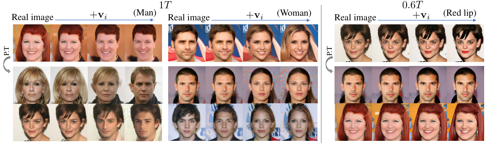
First, we discover the local latent basis for $\mathcal{X}$ and the corresponding local tangent basis for $\mathcal{H}$ . The local basis is obtained by performing singular value decomposition (SVD) of the Jacobian of the mapping from $\mathcal{X}$ to $\mathcal{H}$ . To validate the discovered local latent basis, we demonstrate that walking along the basis can edit real images in a semantically meaningful way. Furthermore, we can use the discovered local latent basis vector to edit other samples by using parallel transport, when they exhibit comparable local geometric structures. Note that existing editing methods manipulate the self-attention map or cross-attention map over multiple timesteps [21, 54, 39]. On the other hand, we manipulate only $\mathbf{x}_{t}$ once at a specific timestep.

Second, we investigate how the latent structures differ across different timesteps and samples as follows. The frequency domain of the local latent basis shifts from low-frequency to high-frequency along the generative process. We explicitly confirm it using power spectral density analysis. The difference between local tangent spaces of different samples becomes larger along the generative process. The local tangent spaces at various diffusion timesteps are similar to each other if the model is trained on aligned datasets such as CelebA-HQ or Flowers. However, this homogeneity does not occur on complex datasets such as ImageNet.

Finally, we examine how the prompts affect the latent structure of text-to-image DMs as follows. Similar prompts yield similar latent structures. Specifically, we find a positive correlation between the similarity of prompts and the similarity of local tangent spaces. The influence of text on the local tangent space becomes weaker along the generative process.

Our work examines the geometry of $\mathcal{X}$ and $\mathcal{H}$ using Riemannian geometry. We discover the latent structure of $\mathcal{X}$ and how it evolves during the generative process and is influenced by prompts. This geometric exploration deepens our understanding of DMs.

2 Related works

Diffusion Models.

Recent advances in DMs make great progress in the field of image synthesis and show state-of-the-art performance [50, 22, 51]. An important subject in the diffusion model is the introduction of gradient guidance, including classifier-free guidance, to control the generative process [17, 47, 4, 30, 36, 46]. The work by Song et al. 2020b has facilitated the unification of DMs with score-based models using SDEs, enhancing our understanding of DMs as a reverse diffusion process. However, the latent space is still largely unexplored, and our understanding is limited.

The study of latent space in GANs.

The study of latent spaces has gained significant attention in recent years. In the field of Generative Adversarial Networks (GANs), researchers have proposed various methods to manipulate the latent space to achieve the desired effect in the generated images [44, 41, 1, 20, 49, 59, 38]. More recently, several studies [60, 10] have examined the geometrical properties of latent space in GANs and utilized these findings for image manipulations. These studies bring the advantage of better understanding the characteristics of the latent space and facilitating the analysis and utilization of GANs. In contrast, the latent space of DMs remains poorly understood, making it difficult to fully utilize their capabilities.

Image manipulation in DMs.

Early works include Choi et al. 2021b and Meng et al. 2021 have attempted to manipulate the resulting images of DMs by replacing latent variables, allowing the generation of desired random images. However, due to the lack of semantics in the latent variables of DMs, current approaches have critical problems with semantic image editing. Alternative approaches have explored the potential of using the feature space within the U-Net for semantic image manipulation. For example, Kwon et al. 2022 have shown that the bottleneck of the U-Net, $\mathcal{H}$ , can be used as a semantic latent space. Specifically, they used CLIP [43] to identify directions within $\mathcal{H}$ that facilitate genuine image editing. Baranchuk et al. 2021 and Tumanyan et al. 2022 use the feature map of the U-Net for semantic segmentation and maintaining the structure of generated images. Unlike previous works, our editing method finds the editing direction without supervision, and directly traverses the latent variable along the latent basis.

Riemannain Geometry.

Some studies have applied Riemannian geometry to analyze the latent spaces of deep generative models, such as Variational Autoencoders (VAEs) and GANs [2, 48, 9, 3, 27, 28, 57]. Shao et al. 2018 proposed a pullback metric on the latent space from image space Euclidean metric to analyze the latent space’s geometry. This method has been widely used in VAEs and GANs because it only requires a differentiable map from latent space to image space. However, no studies have investigated the geometry of latent space of DMs utilizing the pullback metric.

3 Discovering the latent basis of DMs

In this section, we explain how to extract a latent structure of $\mathcal{X}$ using differential geometry. First, we introduce a key concept in our method: the pullback metric. Next, by adopting the local Euclidean metric of $\mathcal{H}$ and utilizing the pullback metric, we discover the local latent basis of the $\mathcal{X}$ . Moreover, although the direction we found is local, we show how it can be applied to other samples via parallel transport. Finally, we introduce $\mathbf{x}$ -space guidance for editing data in the $\mathcal{X}$ to enhance the quality of image generation.

3.1 Pullback metric

We consider a curved manifold, $\mathcal{X}$ , where our latent variables $\mathbf{x}_{t}$ exist. The differential geometry represents $\mathcal{X}$ through patches of tangent spaces, $\mathcal{T}_{\mathbf{x}}{}$ , which are vector spaces defined at each point $\mathbf{x}$ . Then, all the geometrical properties of $\mathcal{X}$ can be obtained from the inner product of $||d\mathbf{x}||^{2}=\langle d{\mathbf{x}},d{\mathbf{x}}\rangle_{\mathbf{x}}$ in $\mathcal{T}_{\mathbf{x}}{}$ . However, we do not have any knowledge of $\langle d{\mathbf{x}},d{\mathbf{x}}\rangle_{\mathbf{x}}$ . It is definitely not a Euclidean metric. Furthermore, samples of $\mathbf{x}_{t}$ at intermediate timesteps of DMs include inevitable noise, which prevents finding semantic directions in $\mathcal{T}_{\mathbf{x}}{}$ .

Fortunately, Kwon et al. 2022 observed that $\mathcal{H}$ , defined by the bottleneck layer of the U-Net, exhibits local linear structure. This allows us to adopt the Euclidean metric on $\mathcal{H}$ . In differential geometry, when a metric is not available on a space, pullback metric is used. If a smooth map exists between the original metric-unavailable domain and a metric-available codomain, the pullback metric is used to measure the distances in the domain space. Our idea is to use the pullback Euclidean metric on $\mathcal{H}$ to define the distances between the samples in $\mathcal{X}$ .

DMs are trained to infer the noise $\mathbf{\epsilon}_{t}$ from a latent variable $\mathbf{x}_{t}$ at each diffusion timestep $t$ . Each $\mathbf{x}_{t}$ has a different internal representation $\mathbf{h}_{t}$ , the bottleneck representation of the U-Net, at different $t$ ’s. The differentiable map between $\mathcal{X}$ and $\mathcal{H}$ is denoted as $f:\mathcal{X}\rightarrow\mathcal{H}$ . Hereafter, we refer to $\mathbf{x}_{t}$ as $\mathbf{x}$ for brevity unless it causes confusion. It is important to note that our method can be applied at any timestep in the denoising process. We consider a linear map, $\mathcal{T}_{\mathbf{x}}{}\rightarrow\mathcal{T}_{\mathbf{h}}{}$ , between the domain and codomain tangent spaces. This linear map can be described by the Jacobian $J_{\mathbf{x}}=\nabla_{\mathbf{x}}\mathbf{h}$ which determines how a vector $\mathbf{v}\in\mathcal{T}_{\mathbf{x}}{}$ is mapped into a vector $\mathbf{u}\in\mathcal{T}_{\mathbf{h}}{}$ by $\mathbf{u}=J_{\mathbf{x}}\mathbf{v}$ .

Using the local linearity of $\mathcal{H}$ , we assume the metric, $||d\mathbf{h}||^{2}=\langle d\mathbf{h},d\mathbf{h}\rangle_{\mathbf{h}}=d\mathbf{h}^{{}^{\mkern-1.5mu\mathsf{T}}}d\mathbf{h}$ as a usual dot product defined in the Euclidean space. To assign a geometric structure to $\mathcal{X}$ , we use the pullback metric of the corresponding $\mathcal{H}$ . In other words, the norm of $\mathbf{v}\in\mathcal{T}_{\mathbf{x}}{}$ is measured by the norm of corresponding codomain tangent vector:

\displaystyle||\mathbf{v}{}||^{2}_{\text{pb}}\triangleq\langle\mathbf{u}{},\mathbf{u}{}\rangle_{\mathbf{h}}=\mathbf{v}{}^{{}^{\mkern-1.5mu\mathsf{T}}}{J}_{\mathbf{x}}{}^{{}^{\mkern-1.5mu\mathsf{T}}}{J}_{\mathbf{x}}{}\mathbf{v}{}.

(1)

3.2 Finding local latent basis

Using the pullback metric, we define the local latent vector $\mathbf{v}\in\mathcal{T}_{\mathbf{x}}{}$ that shows a large variability in $\mathcal{T}_{\mathbf{h}}{}$ . We find a unit vector $\mathbf{v}_{1}$ that maximizes $||\mathbf{v}{}||^{2}_{\text{pb}}$ . By maximizing $||\mathbf{v}{}||^{2}_{\text{pb}}$ while remaining orthogonal to $\mathbf{v}_{1}$ , one can obtain the second unit vector $\mathbf{v}_{2}$ . This process can be repeated to have $n$ latent directions of $\{\mathbf{v}_{1},\mathbf{v}_{2},\cdots,\mathbf{v}_{n}\}$ in $\mathcal{T}_{\mathbf{x}}$ . In practice, $\mathbf{v}_{i}$ corresponds to the $i$ -th right singular vector from the singular value decomposition (SVD) of ${J}_{\mathbf{x}}{}=U\Lambda V^{{}^{\mkern-1.5mu\mathsf{T}}}$ , i.e., $J_{\mathbf{x}}\mathbf{v}_{i}=\Lambda_{i}\mathbf{u}_{i}$ . Since the Jacobian of too many parameters is not tractable, we use a power method [18, 34, 19] to approximate the SVD of ${J}_{\mathbf{x}}{}$ (See Appendix D for the time complexity and Appendix F for the detailed algorithm).

Henceforth, we refer to $\mathcal{T}_{\mathbf{x}}$ as a local latent subspace, and $\{\mathbf{v}_{1},\mathbf{v}_{2},\cdots,\mathbf{v}_{n}\}$ as the corresponding local latent basis.

\displaystyle\mathcal{T}_{\mathbf{x}}\triangleq\text{span}\{\mathbf{v}_{1},\mathbf{v}_{2}\,\cdots,\mathbf{v}_{n}\},~\text{where}~\mathbf{v}_{i}~\text{is}~i\text{-th right singular vector of}~J_{\mathbf{x}}.

(2)

Using the linear transformation between $\mathcal{T}_{\mathbf{x}}{}$ and $\mathcal{T}_{\mathbf{h}}{}$ via the Jacobian ${J}_{\mathbf{x}}{}$ , one can also obtain corresponding directions in $\mathcal{T}_{\mathbf{h}}$ . In practice, $\mathbf{u}_{i}$ corresponds to the $i$ -th left singular vector from the SVD of ${J}_{\mathbf{x}}{}$ . After selecting the top $n$ (e.g., $n=50$ ) directions of large eigenvalues, we can approximate any vector in $\mathcal{T}_{\mathbf{h}}$ with a finite basis, $\{\mathbf{u}_{1},\mathbf{u}_{2},\cdots,\mathbf{u}_{n}\}$ . When we refer to a local tangent space henceforth, it means the $n$ -dimensional low-rank approximation of the original tangent space.

\displaystyle\mathcal{T}_{\mathbf{h}}\triangleq\text{span}\{\mathbf{u}_{1},\mathbf{u}_{2}\,\cdots,\mathbf{u}_{n}\},~\text{where}~\mathbf{u}_{i}~\text{is the}~i\text{-th left singular vector of }~J_{\mathbf{x}}.

(3)

The collection of local latent basis vectors, $\{\mathbf{v}_{1},\mathbf{v}_{2},\cdots,\mathbf{v}_{n}\}$ , obtained through our proposed method, can be interpreted as a signal that the model is highly response to for a given $\mathbf{x}$ . On the other hand, the basis of the local tangent space, denoted as $\{\mathbf{u}_{1},\mathbf{u}_{2}\,\cdots,\mathbf{u}_{n}\}$ , can be viewed as the corresponding representation associated with the signal.

In Stable Diffusion, the prompt also influences the Jacobian, which means that the local basis also depends on it. We can utilize any prompt to obtain a local latent basis, and different prompts create distinct geometrical structures. For the sake of brevity, we will omit the word local unless it leads to confusion.

3.3 Generating edited images with $\mathbf{x}$ -space guidance

A naïve approach for manipulating a latent variable $\mathbf{x}$ using a latent vector $\mathbf{v}$ is through simple addition, specifically $\mathbf{x}+\gamma\mathbf{v}$ . However, using the naïve approach sometime leads to noisy image generation. To address this issue, instead of directly using the basis for manipulation, we use a basis vector that has passed through the decoder once for manipulation. The $\mathbf{x}$ -space guidance is defined as follows

\displaystyle\tilde{\mathbf{x}}_{\text{XG}}=\mathbf{x}+\gamma[\epsilon_{\theta}(\mathbf{x}+\mathbf{v})-\epsilon_{\theta}(\mathbf{x})]

(4)

where $\gamma$ is a hyper-parameter controlling the strength of editing and $\epsilon_{\theta}$ is a diffusion model. Equation 4 is inspired by classifier-free guidance, but the key difference is that it is directly applied in the latent space $\mathcal{X}$ . Our $\mathbf{x}$ -space guidance provides qualitatively similar results to direct addition, while it shows better fidelity. (See Appendix C for ablation study.)

3.4 The overall process of image editing

In this section, we summarize the entire editing process with five steps: 1) The input image is inverted into initial noise $\mathbf{x}_{T}$ using DDIM inversion. 2) $\mathbf{x}_{T}$ is gradually denoised until $t$ through DDIM generation. 3) Identify local latent basis $\{\mathbf{v}_{1},\cdots,\mathbf{v}_{n}\}$ using the pullback metric at $t$ . 4) Manipulate $\mathbf{x}_{t}$ along the one of basis vectors using the $\mathbf{x}$ -space guidance. 5) The DDIM generation is then completed with the modified latent variable $\tilde{\mathbf{x}}_{t}$ . Figure 2 illustrates the entire editing process.

In the context of a text-to-image model, such as Stable Diffusion, it becomes possible to include textual conditions while deriving local basis vectors. Although we do not use any text guidance during DDIM inversion and generation, a local basis with text conditions enables semantic editing that matches the given text. Comprehensive experiments can be found in Section 4.1.

It is noteworthy that our approach needs no extra training and simplifies image editing by only adjusting the latent variable within a single timestep.

3.5 Editing various samples with parallel transport

Let us consider a scenario where our aim is to edit ten images, changing straight hair to curly hair. Due to the nature of the unsupervised image editing method, it is becomes imperative to manually check the semantic relevance of the latent basis vector in the edited results. Thus, to edit every samples, we have to manually find a straight-to-curly basis vector for individual samples.

One way to alleviate this tedious task is to apply the curly hair vector obtained from one image to other images. However, the basis vector $\mathbf{v}\in\mathcal{T}_{\mathbf{x}}{}$ obtained at $\mathbf{x}$ cannot be used for the other sample $\mathbf{x}^{\prime}$ because $\mathbf{v}\notin\mathcal{T}_{\mathbf{x}^{\prime}}$ . Thus, in order to apply the direction we obtained to another sample, it is necessary to relocate the extracted direction to a new tangent space. To achieve this, we use parallel transport that moves $\mathbf{v}_{i}$ onto the new tangent space $\mathcal{T}_{\mathbf{x}^{\prime}}$ .

Parallel transport moves a tangent vector $\mathbf{u}\in\mathcal{T}_{\mathbf{h}}{}$ to $\mathbf{u}^{\prime}\in\mathcal{T}_{\mathbf{h}^{\prime}}$ without changing its direction as much as possible while keeping the vector tangent on the manifold [48]. It is notable that the parallel transport in curved manifold significantly modifies the original vector. Fortunately, $\mathcal{H}$ is relatively flat. Therefore, it is beneficial to apply the parallel transport in $\mathcal{H}$ .

We aims to move $\mathbf{v}_{i}$ onto new tangent space $\mathcal{T}_{\mathbf{x}^{\prime}}$ , using parallel transport in $\mathcal{H}$ . First, we convert the latent direction $\mathbf{v}_{i}\in\mathcal{T}_{\mathbf{x}}$ to the corresponding direction of $\mathbf{u}_{i}\in\mathcal{T}_{\mathbf{h}}$ . Second, we apply the parallel transport $\mathbf{u}_{i}\in\mathcal{T}_{\mathbf{h}}$ to ${\mathbf{u}^{\prime}}_{i}\in\mathcal{T}_{\mathbf{h}^{\prime}}$ , where $\mathbf{h}^{\prime}=f(\mathbf{x}^{\prime})$ . In the general case, parallel transport involves iterative projection and normalization on the tangent space along the path connecting two points [48]. However, in our case, we assume that $\mathcal{H}$ has Euclidean geometry. Therefore, we move $\mathbf{u}$ directly onto $\mathcal{T}_{\mathbf{h}^{\prime}}$ through projection, without the need for an iterative process. Finally, transform $\mathbf{u}^{\prime}_{i}$ into $\mathbf{v}^{\prime}_{i}\in\mathcal{X}$ . Using this parallel transport of $\mathbf{v}_{i}\to\mathbf{v}^{\prime}_{i}$ via $\mathcal{H}$ , we can apply the local latent basis obtained from $\mathbf{x}$ to edit or modify the input $\mathbf{x}^{\prime}$ .

4 Findings and results

In this section, we analyze the geometric structure of DMs with our method. $\lx@sectionsign$ 4.1 demonstrates that the latent basis found by our method can be used for image editing. In $\lx@sectionsign$ 4.2, we investigate how the geometric structure of DMs evolves as the generative process progresses. Lastly, in $\lx@sectionsign$ 4.3, we examine how the geometric properties of the text-condition model change with a given text.

The implementation details of our work are provided on Appendix B. The source code for our experiments is included in the supplementary materials and will be publicly available upon publication.

4.1 Image editing with the latent basis

In this subsection, we demonstrate the capability of our discovered latent basis for image editing. To extract the latent variables from real images for editing purposes, we use DDIM inversion. In experiments with Stable Diffusion (SD), we do not use guidance, i.e., unconditional sampling, for both DDIM inversion and DDIM sampling processes. This ensures that our editing results solely depend on the latent variable, not on other factors such as prompt conditions.

Figures 2 and 3 illustrate the example results edited by the latent basis found by our method. The latent basis clearly contains semantics such as age, gender, species, structure, and texture. Note that editing at timestep $T$ yields coarse changes such as age and species. On the other hand, editing at timestep $0.6T$ leads to fine changes, such as nose color and facial expression.

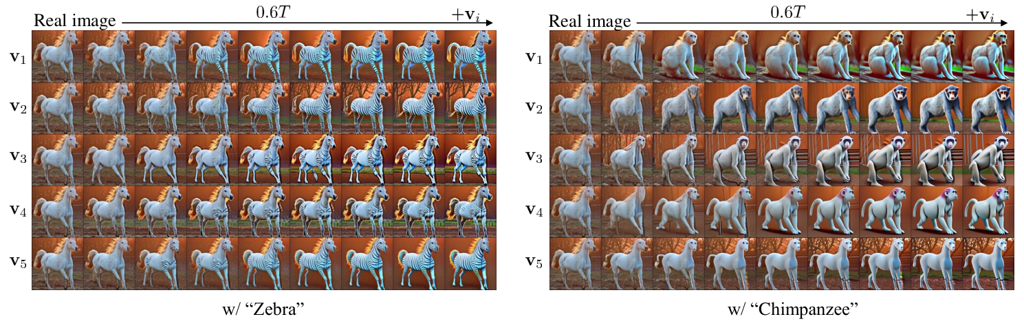
Figure 4 demonstrates the example results edited by the various latent basis vectors. Interestingly, using the text “lion” as a condition, the entire latent basis captures lion-related attributes. Furthermore, Figure 5 shows that the latent basis aligns with the text not only in terms of object types but also in relation to pose or action. For a qualitative comparison with other state-of-the-art image editing methods, refer to Appendix D. For more examples of editing results, refer to Appendix G.

4.2 Evolution of latent structures during generative processes

In this subsection, we demonstrate how the latent structure evolves during the generative process and identify three trends. 1) The frequency domain of the latent basis changes from low to high frequency. It agrees with the previous observation that DMs generate samples in coarse-to-fine manner. 2) The difference between the tangent spaces of different samples increases over the generative process. It implies finding generally applicable editing direction in latent space becomes harder in later timesteps. 3) The differences of tangent spaces between timesteps depend on the complexity of the dataset.

Latent bases gradually evolve from low- to high-frequency structures.

Figure 6 is the power spectral density (PSD) of the discovered latent basis over various timesteps. The early timesteps contain a larger portion of low frequency than the later timesteps and the later timesteps contain a larger portion of high frequency.

This suggests that the model focuses on low-frequency signals at the beginning of the generative process and then shifts its focus to high-frequency signals over time. This result strengthens the common understanding about the coarse-to-fine behavior of DMs over the generative process [12, 15].

The discrepancy of tangent spaces from different samples increases along the generative process.

To investigate the geometry of the tangent basis, we employ a metric on the Grassmannian manifold. The Grassmannian manifold is a manifold where each point is a vector space, and the metric defined above represents the distortion across various vector spaces. We use geodesic metric [10, 56] to define the discrepancy between two subspaces $\{\mathcal{T}^{(1)},\mathcal{T}^{(2)}\}$ :

D_{\text{geo}}(\mathcal{T}^{(1)},\mathcal{T}^{(2)})=\sqrt{\sum_{k}\theta_{k}^{2}},

(5)

where $\theta_{k}$ denotes the $k$ -th principle angle between $\mathcal{T}^{(1)}$ and $\mathcal{T}^{(2)}$ . Intuitively, the concept of geodesic metric can be understood as an angle between two vector spaces. Here, the comparison between two different spaces was conducted for $\{\mathcal{T}_{\mathbf{h}_{1}},\mathcal{T}_{\mathbf{h}_{2}}\}$ . Unlike the $\mathcal{X}$ , the $\mathcal{H}$ assumes a Euclidean space which makes the computation of geodesic metric that requires an inner product between tangent spaces easier. The relationship between tangent space and latent subspace is covered in more detail in Appendix E.

Figure 7 demonstrates that the tangent spaces of the different samples are the most similar at $t=T$ and diverge as timestep becomes zero.

Moreover, the similarity across tangent spaces allows us to effectively transfer the latent basis from one sample to another through parallel transport as shown in Figure 8. In $T$ , where the tangent spaces are homogeneous, we consistently obtain semantically aligned editing results. On the other hand, parallel transport at $t=0.6T$ does not lead to satisfactory editing because the tangent spaces are hardly homogeneous. Thus, we should examine the similarity of local subspaces to ensure consistent editing across samples.

DMs trained on simpler datasets exhibit more consistent tangent spaces over time.

In Figure 9 (a), we provide a distance matrix of the tangent spaces across different timesteps, measured by the geodesic metric. We observe that the tangent spaces are more similar to each other when a model is trained on CelebA-HQ, compared to ImageNet. To verify this trend, we measure the geodesic distances between tangent spaces of different timesteps and plot the average distances of the same difference in timestep in Figure 9 (b). As expected, we find that DMs trained on datasets, that are generally considered simpler, have similar local tangent spaces over time.

4.3 Effect of conditioning prompts on the latent structure

In this subsection, we aim to investigate how prompts influence the generative process from a geometrical perspective. We randomly sampled 50 captions from the MS-COCO dataset [29] and used them as text conditions.

Similar text conditions induce similar tangent spaces.

In Figure 10 (a), we observe a negative correlation between the CLIP similarity of texts and the distance between tangent spaces. In other words, when provided with similar texts, the tangent spaces are more similar. The linear relationship between the text and the discrepancy of the tangent spaces is particularly strong in the early phase of the generative process as shown by $R^{2}$ score in Figure 10 (b).

The generative process depends less on text conditions in later timesteps.

Figure 10 (c) illustrates the distances between local tangent spaces for given different prompts with respect to the timesteps. Notably, as the diffusion timestep approaches values below $0.7T$ , the distances between the local tangent spaces start to decrease. It implies that the variation due to walking along the local tangent basis depends less on the text conditions, i.e., the text less influences the generative process, in later timesteps. It is a possible reason why the correlation between the similarity of prompts and the similarity of tangent spaces reduces over timesteps.

5 Discussion

In this section, we provide additional intuitions and implications. It is interesting that our latent basis usually conveys disentangled attributes even though we do not adopt attribute annotation to enforce disentanglement. We suppose that decomposing the Jacobian of the encoder in the U-Nets naturally yields disentanglement to some extent. However, it does not guarantee the perfect disentanglement and some directions are entangled. For example, the editing for beard converts a female subject to a male as shown in Figure 11 (a). This kind of entanglement often occurs in other editing methods due to the dataset bias: female faces seldom have beard.

While our method has shown effectiveness in Stable Diffusion, more research is needed to fully validate its potential. We have observed that some of the discovered latent vector occasionally leads to abrupt changes during the editing process in Stable Diffusion, as depicted in Figure 11 (b). This observation highlights the complex geometry of $\mathcal{X}$ in achieving seamless editing. Exploring this topic in future research is an interesting area to delve into.

Our approach is broadly applicable when the feature space in the DM adheres to a Euclidean metric, as demonstrated by $\mathcal{H}$ . This characteristic has been observed in the context of U-Net within Kwon et al. 2022. It would be intriguing to investigate if other architectural designs, especially those similar to transformer structures as introduced in [42, 53], also exhibit a Euclidean metric.

Despite these limitations, our method provides a significant advance in the field of image editing for DMs, and provides a deep understanding of DM through several experiments.

6 Conclusion

We have analyzed the latent space of DMs from a geometrical perspective. We used the pullback metric to identify the latent and tangent bases in $\mathcal{X}$ and $\mathcal{H}$ . The latent basis found by the pullback metric allows editing images by traversal along the basis. We have observed properties of the bases in two aspects. First, we discovered that 1) the latent bases evolve from low- to high-frequency components; 2) the discrepancy of tangent spaces from different samples increases along the generative process; and 3) DMs trained on simpler datasets exhibit more consistent tangent spaces over timesteps. Second, we investigated how the latent structure changes based on the text conditions in Stable Diffusion, and discovered that similar prompts make tangent space analogous but its effect becomes weaker over timesteps. We believe that a better understanding of the geometry of DMs will open up new possibilities for adopting DMs in useful applications.

7 Acknowledgement

This work was supported in part by the Creative-Pioneering Researchers Program through Seoul National University, the National Research Foundation of Korea (NRF) grant (Grant No. 2022R1A2C1006871) (J. J.), KIAS Individual Grant [AP087501] via the Center for AI and Natural Sciences at Korea Institute for Advanced Study, and the National Research Foundation of Korea (NRF) grant (RS-2023-00223062).

References

Abdal et al. [2021] Rameen Abdal, Peihao Zhu, Niloy J Mitra, and Peter Wonka. Styleflow: Attribute-conditioned exploration of stylegan-generated images using conditional continuous normalizing flows. ACM Transactions on Graphics (ToG), 40(3):1–21, 2021.
Arvanitidis et al. [2017] Georgios Arvanitidis, Lars Kai Hansen, and Søren Hauberg. Latent space oddity: on the curvature of deep generative models. arXiv preprint arXiv:1710.11379, 2017.
Arvanitidis et al. [2020] Georgios Arvanitidis, Søren Hauberg, and Bernhard Schölkopf. Geometrically enriched latent spaces. arXiv preprint arXiv:2008.00565, 2020.
Avrahami et al. [2022] Omri Avrahami, Dani Lischinski, and Ohad Fried. Blended diffusion for text-driven editing of natural images. In Proceedings of the IEEE/CVF Conference on Computer Vision and Pattern Recognition, pages 18208–18218, 2022.
Balaji et al. [2022] Yogesh Balaji, Seungjun Nah, Xun Huang, Arash Vahdat, Jiaming Song, Karsten Kreis, Miika Aittala, Timo Aila, Samuli Laine, Bryan Catanzaro, et al. ediffi: Text-to-image diffusion models with an ensemble of expert denoisers. arXiv preprint arXiv:2211.01324, 2022.
Baranchuk et al. [2021] Dmitry Baranchuk, Ivan Rubachev, Andrey Voynov, Valentin Khrulkov, and Artem Babenko. Label-efficient semantic segmentation with diffusion models. arXiv preprint arXiv:2112.03126, 2021.
Brooks et al. [2023] Tim Brooks, Aleksander Holynski, and Alexei A Efros. Instructpix2pix: Learning to follow image editing instructions. In Proceedings of the IEEE/CVF Conference on Computer Vision and Pattern Recognition, pages 18392–18402, 2023.
Chefer et al. [2023] Hila Chefer, Yuval Alaluf, Yael Vinker, Lior Wolf, and Daniel Cohen-Or. Attend-and-excite: Attention-based semantic guidance for text-to-image diffusion models. arXiv preprint arXiv:2301.13826, 2023.
Chen et al. [2018] Nutan Chen, Alexej Klushyn, Richard Kurle, Xueyan Jiang, Justin Bayer, and Patrick Smagt. Metrics for deep generative models. In International Conference on Artificial Intelligence and Statistics, pages 1540–1550. PMLR, 2018.
Choi et al. [2021a] Jaewoong Choi, Junho Lee, Changyeon Yoon, Jung Ho Park, Geonho Hwang, and Myungjoo Kang. Do not escape from the manifold: Discovering the local coordinates on the latent space of gans. arXiv preprint arXiv:2106.06959, 2021a.
Choi et al. [2021b] Jooyoung Choi, Sungwon Kim, Yonghyun Jeong, Youngjune Gwon, and Sungroh Yoon. Ilvr: Conditioning method for denoising diffusion probabilistic models. arXiv preprint arXiv:2108.02938, 2021b.
Choi et al. [2022] Jooyoung Choi, Jungbeom Lee, Chaehun Shin, Sungwon Kim, Hyunwoo Kim, and Sungroh Yoon. Perception prioritized training of diffusion models. In Proceedings of the IEEE/CVF Conference on Computer Vision and Pattern Recognition, pages 11472–11481, 2022.
Choi et al. [2020] Yunjey Choi, Youngjung Uh, Jaejun Yoo, and Jung-Woo Ha. Stargan v2: Diverse image synthesis for multiple domains. In Proceedings of the IEEE/CVF conference on computer vision and pattern recognition, pages 8188–8197, 2020.
Chung et al. [2022] Hyungjin Chung, Byeongsu Sim, Dohoon Ryu, and Jong Chul Ye. Improving diffusion models for inverse problems using manifold constraints. arXiv preprint arXiv:2206.00941, 2022.
Daras and Dimakis [2022] Giannis Daras and Alexandros G Dimakis. Multiresolution textual inversion. arXiv preprint arXiv:2211.17115, 2022.
Deng et al. [2009] Jia Deng, Wei Dong, Richard Socher, Li-Jia Li, Kai Li, and Li Fei-Fei. Imagenet: A large-scale hierarchical image database. In 2009 IEEE conference on computer vision and pattern recognition, pages 248–255. Ieee, 2009.
Dhariwal and Nichol [2021] Prafulla Dhariwal and Alexander Nichol. Diffusion models beat gans on image synthesis. Advances in Neural Information Processing Systems, 34:8780–8794, 2021.
Golub and Van Loan [2013] Gene H Golub and Charles F Van Loan. Matrix computations. JHU press, 2013.
Haas et al. [2023] René Haas, Inbar Huberman-Spiegelglas, Rotem Mulayoff, and Tomer Michaeli. Discovering interpretable directions in the semantic latent space of diffusion models. arXiv preprint arXiv:2303.11073, 2023.
Härkönen et al. [2020] Erik Härkönen, Aaron Hertzmann, Jaakko Lehtinen, and Sylvain Paris. Ganspace: Discovering interpretable gan controls. Advances in Neural Information Processing Systems, 33:9841–9850, 2020.
Hertz et al. [2022] Amir Hertz, Ron Mokady, Jay Tenenbaum, Kfir Aberman, Yael Pritch, and Daniel Cohen-Or. Prompt-to-prompt image editing with cross attention control. arXiv preprint arXiv:2208.01626, 2022.
Ho et al. [2020] Jonathan Ho, Ajay Jain, and Pieter Abbeel. Denoising diffusion probabilistic models. Advances in Neural Information Processing Systems, 33:6840–6851, 2020.
Karras et al. [2018] Tero Karras, Timo Aila, Samuli Laine, and Jaakko Lehtinen. Progressive growing of gans for improved quality, stability, and variation. In International Conference on Learning Representations, 2018.
Karras et al. [2019] Tero Karras, Samuli Laine, and Timo Aila. A style-based generator architecture for generative adversarial networks. In Proceedings of the IEEE/CVF conference on computer vision and pattern recognition, pages 4401–4410, 2019.
Karras et al. [2022] Tero Karras, Miika Aittala, Timo Aila, and Samuli Laine. Elucidating the design space of diffusion-based generative models. arXiv preprint arXiv:2206.00364, 2022.
Kwon et al. [2022] Mingi Kwon, Jaeseok Jeong, and Youngjung Uh. Diffusion models already have a semantic latent space. arXiv preprint arXiv:2210.10960, 2022.
Lee and Park [2023] Yonghyeon Lee and Frank C Park. On explicit curvature regularization in deep generative models. 2023.
Lee et al. [2022] Yonghyeon Lee, Seungyeon Kim, Jinwon Choi, and Frank Park. A statistical manifold framework for point cloud data. In Kamalika Chaudhuri, Stefanie Jegelka, Le Song, Csaba Szepesvari, Gang Niu, and Sivan Sabato, editors, Proceedings of the 39th International Conference on Machine Learning, volume 162 of Proceedings of Machine Learning Research, pages 12378–12402. PMLR, 17–23 Jul 2022. URL https://proceedings.mlr.press/v162/lee22d.html.
Lin et al. [2014] Tsung-Yi Lin, Michael Maire, Serge Belongie, James Hays, Pietro Perona, Deva Ramanan, Piotr Dollár, and C Lawrence Zitnick. Microsoft coco: Common objects in context. In Computer Vision–ECCV 2014: 13th European Conference, Zurich, Switzerland, September 6-12, 2014, Proceedings, Part V 13, pages 740–755. Springer, 2014.
Liu et al. [2021] Xihui Liu, Dong Huk Park, Samaneh Azadi, Gong Zhang, Arman Chopikyan, Yuxiao Hu, Humphrey Shi, Anna Rohrbach, and Trevor Darrell. More control for free! image synthesis with semantic diffusion guidance. arXiv preprint arXiv:2112.05744, 2021.
Lugmayr et al. [2022] Andreas Lugmayr, Martin Danelljan, Andres Romero, Fisher Yu, Radu Timofte, and Luc Van Gool. Repaint: Inpainting using denoising diffusion probabilistic models. In Proceedings of the IEEE/CVF Conference on Computer Vision and Pattern Recognition, pages 11461–11471, 2022.
Ma et al. [2023] Chaofan Ma, Yuhuan Yang, Chen Ju, Fei Zhang, Jinxiang Liu, Yu Wang, Ya Zhang, and Yanfeng Wang. Diffusionseg: Adapting diffusion towards unsupervised object discovery. arXiv preprint arXiv:2303.09813, 2023.
Meng et al. [2021] Chenlin Meng, Yang Song, Jiaming Song, Jiajun Wu, Jun-Yan Zhu, and Stefano Ermon. Sdedit: Image synthesis and editing with stochastic differential equations. arXiv preprint arXiv:2108.01073, 2021.
Miyato et al. [2018] Takeru Miyato, Toshiki Kataoka, Masanori Koyama, and Yuichi Yoshida. Spectral normalization for generative adversarial networks. arXiv preprint arXiv:1802.05957, 2018.
Mokady et al. [2022] Ron Mokady, Amir Hertz, Kfir Aberman, Yael Pritch, and Daniel Cohen-Or. Null-text inversion for editing real images using guided diffusion models. arXiv preprint arXiv:2211.09794, 2022.
Nichol et al. [2021] Alex Nichol, Prafulla Dhariwal, Aditya Ramesh, Pranav Shyam, Pamela Mishkin, Bob McGrew, Ilya Sutskever, and Mark Chen. Glide: Towards photorealistic image generation and editing with text-guided diffusion models. arXiv preprint arXiv:2112.10741, 2021.
Nichol and Dhariwal [2021] Alexander Quinn Nichol and Prafulla Dhariwal. Improved denoising diffusion probabilistic models. In International Conference on Machine Learning, pages 8162–8171. PMLR, 2021.
Pan et al. [2023] Xingang Pan, Ayush Tewari, Thomas Leimkühler, Lingjie Liu, Abhimitra Meka, and Christian Theobalt. Drag your gan: Interactive point-based manipulation on the generative image manifold. In ACM SIGGRAPH 2023 Conference Proceedings, pages 1–11, 2023.
Parmar et al. [2023] Gaurav Parmar, Krishna Kumar Singh, Richard Zhang, Yijun Li, Jingwan Lu, and Jun-Yan Zhu. Zero-shot image-to-image translation. arXiv preprint arXiv:2302.03027, 2023.
Paszke et al. [2017] Adam Paszke, Sam Gross, Soumith Chintala, Gregory Chanan, Edward Yang, Zachary DeVito, Zeming Lin, Alban Desmaison, Luca Antiga, and Adam Lerer. Automatic differentiation in pytorch. In NIPS-W, 2017.
Patashnik et al. [2021] Or Patashnik, Zongze Wu, Eli Shechtman, Daniel Cohen-Or, and Dani Lischinski. Styleclip: Text-driven manipulation of stylegan imagery. In Proceedings of the IEEE/CVF International Conference on Computer Vision, pages 2085–2094, 2021.
Peebles and Xie [2023] William Peebles and Saining Xie. Scalable diffusion models with transformers. In Proceedings of the IEEE/CVF International Conference on Computer Vision, pages 4195–4205, 2023.
Radford et al. [2021] Alec Radford, Jong Wook Kim, Chris Hallacy, Aditya Ramesh, Gabriel Goh, Sandhini Agarwal, Girish Sastry, Amanda Askell, Pamela Mishkin, Jack Clark, et al. Learning transferable visual models from natural language supervision. In International Conference on Machine Learning, pages 8748–8763. PMLR, 2021.
Ramesh et al. [2018] Aditya Ramesh, Youngduck Choi, and Yann LeCun. A spectral regularizer for unsupervised disentanglement. arXiv preprint arXiv:1812.01161, 2018.
Ramesh et al. [2022] Aditya Ramesh, Prafulla Dhariwal, Alex Nichol, Casey Chu, and Mark Chen. Hierarchical text-conditional image generation with clip latents. arXiv preprint arXiv:2204.06125, 2022.
Rombach et al. [2022] Robin Rombach, Andreas Blattmann, Dominik Lorenz, Patrick Esser, and Björn Ommer. High-resolution image synthesis with latent diffusion models. In Proceedings of the IEEE/CVF Conference on Computer Vision and Pattern Recognition, pages 10684–10695, 2022.
Sehwag et al. [2022] Vikash Sehwag, Caner Hazirbas, Albert Gordo, Firat Ozgenel, and Cristian Canton. Generating high fidelity data from low-density regions using diffusion models. In Proceedings of the IEEE/CVF Conference on Computer Vision and Pattern Recognition, pages 11492–11501, 2022.
Shao et al. [2018] Hang Shao, Abhishek Kumar, and P Thomas Fletcher. The riemannian geometry of deep generative models. In Proceedings of the IEEE Conference on Computer Vision and Pattern Recognition Workshops, pages 315–323, 2018.
Shen and Zhou [2021] Yujun Shen and Bolei Zhou. Closed-form factorization of latent semantics in gans. In Proceedings of the IEEE/CVF Conference on Computer Vision and Pattern Recognition, pages 1532–1540, 2021.
Sohl-Dickstein et al. [2015] Jascha Sohl-Dickstein, Eric Weiss, Niru Maheswaranathan, and Surya Ganguli. Deep unsupervised learning using nonequilibrium thermodynamics. In International Conference on Machine Learning, pages 2256–2265. PMLR, 2015.
Song et al. [2020a] Jiaming Song, Chenlin Meng, and Stefano Ermon. Denoising diffusion implicit models. arXiv preprint arXiv:2010.02502, 2020a.
Song et al. [2020b] Yang Song, Jascha Sohl-Dickstein, Diederik P Kingma, Abhishek Kumar, Stefano Ermon, and Ben Poole. Score-based generative modeling through stochastic differential equations. arXiv preprint arXiv:2011.13456, 2020b.
Tevet et al. [2022] Guy Tevet, Sigal Raab, Brian Gordon, Yonatan Shafir, Daniel Cohen-Or, and Amit H Bermano. Human motion diffusion model. arXiv preprint arXiv:2209.14916, 2022.
Tumanyan et al. [2022] Narek Tumanyan, Michal Geyer, Shai Bagon, and Tali Dekel. Plug-and-play diffusion features for text-driven image-to-image translation. arXiv preprint arXiv:2211.12572, 2022.
Xu et al. [2023] Jiarui Xu, Sifei Liu, Arash Vahdat, Wonmin Byeon, Xiaolong Wang, and Shalini De Mello. Open-vocabulary panoptic segmentation with text-to-image diffusion models. arXiv preprint arXiv:2303.04803, 2023.
Ye and Lim [2016] Ke Ye and Lek-Heng Lim. Schubert varieties and distances between subspaces of different dimensions. SIAM Journal on Matrix Analysis and Applications, 37(3):1176–1197, 2016.
Yonghyeon et al. [2021] LEE Yonghyeon, Sangwoong Yoon, MinJun Son, and Frank C Park. Regularized autoencoders for isometric representation learning. In International Conference on Learning Representations, 2021.
Yu et al. [2015] Fisher Yu, Ari Seff, Yinda Zhang, Shuran Song, Thomas Funkhouser, and Jianxiong Xiao. Lsun: Construction of a large-scale image dataset using deep learning with humans in the loop. arXiv preprint arXiv:1506.03365, 2015.
Yüksel et al. [2021] Oğuz Kaan Yüksel, Enis Simsar, Ezgi Gülperi Er, and Pinar Yanardag. Latentclr: A contrastive learning approach for unsupervised discovery of interpretable directions. In Proceedings of the IEEE/CVF International Conference on Computer Vision, pages 14263–14272, 2021.
Zhu et al. [2021] Jiapeng Zhu, Ruili Feng, Yujun Shen, Deli Zhao, Zheng-Jun Zha, Jingren Zhou, and Qifeng Chen. Low-rank subspaces in gans. Advances in Neural Information Processing Systems, 34:16648–16658, 2021.

Appendix A Societal Impacts & Ethics Statements

Our research endeavors to unravel the geometric structures of the diffusion model and facilitate high-quality image editing within its framework. While our primary application resides within the creative realm, it is important to acknowledge that image manipulation techniques, such as the one proposed in our method, hold the potential for misuse, including the dissemination of misinformation or potential privacy implications. Therefore, the continuous advancement of technologies aimed at thwarting or identifying manipulations rooted in generative models remains of utmost significance.

Appendix B Implementation details

Models and datasets

We validate our method and provide analyses on various models using the official code and pre-trained checkpoints. The available combinations of the models and the datasets are: DDPM [22] on ImageNet [16], LSUN-church/bedroom/cat/horse [58], and CelebA-HQ [23]; and DDPM trained with P2 weighting [12] on FFHQ [24], Flowers [58] and AFHQ [13]. We also use Stable Diffusion (SD) version 2.1 [46] for the text-conditional diffusion model.

For image editing, we use the official codes and pre-trained checkpoints for all baselines and keep the parameters frozen. For analysis, we compare models with the same diffusion scheduling (linear schedule) and resolutions ( $256^{2}$ ) to ensure a fair comparison, except Stable Diffusion.

Table A11 summarizes various hyperparameter settings in our experiments. Specific details not covered in the main text are discussed in the following paragraphs.

Edit timestep ( $t_{edit}$ )

For unconditional DMs, we show the editing results at $t_{edit}\in\{T,0.8T,0.6T\}$ , while for Stable Diffusion, we show the editing results at $t_{edit}\in\{0.7T,0.6T\}$ . Note that our method allows manipulation at any timestep.

Inversion step

We conduct real image editing with DDIM inversion [51]. We set the number of steps to $100$ for obtaining the latent variable $\mathbf{x}_{T}$ and all experiments.

$\mathbf{x}$ -space guidance scale ( $\gamma$ )

The value of $\gamma$ determines the magnitude of a single editing step by $\mathbf{x}$ -space guidance. Fortunately, through experimentation, we observed that the value of $\gamma$ does not have a significant impact on image quality unless it is excessively large.

Low-rank approximation ( $n$ )

We employ a low-rank approximation of the tangent space using $n=50$ for all settings.

Quality boosting ( $t_{boost}$ )

While DDIM alone already generates high-quality images, Karras et al. 2022 showed that including stochasticity in the process improves image quality and Kwon et al. 2022 suggest similar technique: adding stochasticity at the end of the generative process. We employ this technique in our experiments on every experiment after $t=0.2T$ , except Stable Diffusion.

Computing resource

For power-method approximation with $n=50$ , it spends about 3-4 minutes on a single NVIDIA RTX 3090 (24GB). As $n$ specifies the number of bases, it can be as small as a user want to use for image editing. Reducing $n$ provides faster runtime, e.g., 10 seconds for $n=3$ .

Table A1: Hyper-parameter settings.

model	$t_{edit}$	inversion step	$\gamma$	$n$	$t_{boost}$
Stable Diffusion	$0.7T$	100	1	50	$\times$
	$0.6T$	100	2	50	$\times$
Unconditional DMs	$T$	100	0.5	50	$0.2T$
	$0.8T$	100	1	50	$0.2T$
	$0.6T$	100	4	50	$0.2T$

Appendix C Ablation study

In this section, we validate our method with ablation study.

Random $\mathbf{v}$

To demonstrate the meaningfulness of the latent basis found by our method, we qualitatively compare its effect to naïve baseline: random directions. The first row in Figure A1 shows that manipulating the images with a random vector ‘ $\mathbf{v}$ ’ does not result in semantic editing but rather degrades images. The second row shows the results of projecting the random ‘ $\mathbf{v}$ ’ onto our obtained latent subspace. The projected results exhibit semantic manipulation such as pose changes without image distortion. It indicates that the found latent subspace captures semantics in the latent space effectively.

$\mathbf{x}$ -space guidance

Figure A2 demonstrates the the effectiveness of $\mathbf{x}$ -space guidance compared to a straightforward alternative: simple addition. First, $\mathbf{x}$ -space guidance produces higher quality images with similar meaning. Especially Stable Diffusion apparently benefits from $\mathbf{x}$ -space guidance regarding smoothness of the editing strength and artifacts. The difference is more significant at $t=0.6T$ . Note that the meaning of the same directions may slightly differ between the two settings due to non-linearity of the U-Net.

Currently, we do not have a deeper understanding of the underlying principles of $\mathbf{x}$ -space guidance. Exploring the reasons behind its ability to improve manipulation quality would be an interesting direction for future work.

Appendix D Comparative experiment to other state-of-the-art (SoTA) editing methods

We conduct qualitative comparisons with text-guided image editing methods. Our SoTA baseline methods include: (i) SDEdit [33], (ii) Pix2Pix-zero [39], (iii) PnP [54], and (iv) Instruct Pix2Pix [7]. All comparisons were performed using the official code. Please refer to Figure A3 for the qualitative results.

We also compare the time complexity of each method. For a fair comparison, we only identify the first singular vector $\mathbf{v}_{1}$ , i.e., $n=1$ , and set the number of DDIM steps to 50. All experiments were conducted on an Nvidia RTX 3090. The runtime for each method is summarized in Table A2.

The computation cost of our method remains comparable to other approaches, although the Jacobian approximation takes around 2.5 seconds for $n=1$ . This is because we only need to identify the latent basis vector once at a specific timestep. Furthermore, our approach does not require additional preprocessing steps like generating 100 prompts with GPT and obtaining embedding vectors (as in Pix2Pix-zero), or storing feature vectors, queries, and key values (as in PnP). Our method also does not require finetuning (as in Instruct Pix2Pix). This leads to a significantly reduced total editing process time in comparison to other methods.

Table A2: Comparisons of the time complexity of state-of-the-art editing methods

Image Edit Method	Running time	Preprocessing
Ours	11 sec	N/A
SDEdit	4 sec	N/A
Pix2Pix-zero	25 sec	4 min
PnP	10 sec	40 sec
Instruct Pix2Pix	11 sec	N/A

Appendix E More Discussions

Why do we measure the geodesic distance of the tangent spaces instead of the latent subspaces?

The geodesic distance on the Grassmannian manifold between two subspaces is defined as the $l_{2}$ -norm of principal angles. To define angles between different vector spaces, an inner product needs to be defined. In our work, we define the inner product in $\mathcal{T}_{\mathbf{x}}$ using the pullback metric. The issue is that the pullback metric is locally defined for each latent subspace $\mathcal{T}_{\mathbf{x}}$ (Eq. (1)). Therefore, measuring angles between distant latent subspaces becomes challenging. On the other hand, $\mathcal{H}$ follows the assumption of the Euclidean metric. Consequently, even for distant tangent spaces, angles can be easily computed using the dot product. In this regard, we measure the similarity between latent subspaces by exploiting the geodesic distance of their corresponding tangent spaces. Furthermore, when compared to $\mathcal{X}$ , $\mathcal{H}$ offers the advantage of being a semantic space, making it more suitable for measuring semantic similarity.

Similar tangent space implies similar latent subspace

In Figure A4, we calculated the geodesic distance of tangent spaces obtained at different timesteps (or different samples at same the timestep) and the angle between the original latent direction and parallel transported direction between them. It is evident that as the geodesic distance decreases, the amount of distortion during parallel transport also reduces.

Notice that the similarity between tangent spaces implies consistency of latent basis across timesteps. In Figure A5 (b), we parallel transport the latent vector $\mathbf{v}_{i}$ to various tangent spaces and visualize the outcomes. As expected, when the tangent spaces are similar, the transported vector ${\mathbf{v}^{\prime}}_{i}$ retains the original signal. On the other hand, as we move to more distant timesteps, where the tangent space is farther apart, ${\mathbf{v}^{\prime}}_{i}$ deviates from the original signal.

Appendix F Algorithms

In this section, for reproducibility purposes, we provide the code for two important algorithms. The code is implemented using PyTorch [40].

Jacobian subspace iteration

The diffusion model has dimensions that are too large in both $\mathcal{X}$ and $\mathcal{H}$ , making the computation of the Jacobian infeasible. To overcome this challenge, we attempt the Jacobian subspace iteration algorithm to approximate the singular value of the Jacobian, as proposed in [19]. For details, please refer to Haas et al. 2023.

⬇

1 import torch # >= ver 2.0

3 def local_encoder_pullback(

4 x, t, get_h, n=50, chunk_size=25, min_iter=10, max_iter=100, convergence_threshold=1e-4,

5 ):

6 ’’’

7 Args

8 - x : tensor ; latent variable

9 - t : tensor ; diffusion timestep

10 - get_h : function ; return h given x, t

11 - n ; low-rank approximation dimension

12 - chunk_size ; To avoid OOM error

13 - min_iter (max_iter) ; minimum (maximum) number of iteration

14 - convergence_threshold ; to check convergence of power-method

15 ’’’

16 # set number of chunk to avoid OOM

17 num_chunk = n // chunk_size + 1

19 # get dimensions of x space and h space

20 h_shape = get_h(x, t).shape

21 c_i, w_i, h_i = x.size(1), x.size(2), x.size(3)

22 c_o, w_o, h_o = h_shape[1], h_shape[2], h_shape[3]

24 # power-method

25 a = torch.tensor(0., device=x.device, dtype=x.dtype)

26 vT = torch.randn(c_i*w_i*h_i, n, device=x.device)

27 vT, _ = torch.linalg.qr(vT)

28 v = vT.T

29 v = v.view(-1, c_i, w_i, h_i)

31 for i in range(max_iter):

32 v = v.to(device=x.device, dtype=x.dtype)

33 v_prev = v.detach().cpu().clone()

35 time_s = time.time()

36 u = []

37 v_buffer = list(v.chunk(num_chunk))

38 for vi in v_buffer:

39 g = lambda a : get_h(x + a*vi, t=t)

40 ui = torch.func.jacfwd(

41 g, argnums=0, has_aux=False, randomness=’error’

42 )(a)

43 u.append(ui.detach().cpu().clone())

44 u = torch.cat(u, dim=0)

45 u = u.to(x.device, x.dtype)

47 g = lambda x : torch.einsum(

48 ’b c w h, i c w h -> b’, u, get_h(x, t=t)

49 )

50 v_ = torch.autograd.functional.jacobian(g, x)

51 v_ = v_.view(-1, c_i*w_i*h_i)

53 _, s, v = torch.linalg.svd(v_, full_matrices=False)

54 v = v.view(-1, c_i, w_i, h_i)

55 u = u.view(-1, c_o, w_o, h_o)

57 convergence = torch.dist(v_prev, v.detach().cpu()).item()

58 if torch.allclose(v_prev, v.detach().cpu(), atol=convergence_threshold) and (i > min_iter):

59 break

61 # reshape as a x space, h space vector

62 u, s, vT = u.reshape(-1, c_o*w_o*h_o).T.detach(), s.sqrt().detach(), v.reshape(-1, c_i*w_i*h_i).detach()

63 return u, s, vT

Listing 1: Jacobian subspace iteration

Geodesic metric

For a detailed discussion on the geodesic metric, please refer to Choi et al. 2021a for more information.

⬇

1 import torch

3 def geodesic_metric(U1, U2):

4 _, S, _ = torch.linalg.svd(U1.T @ U2)

5 th = torch.acos(S)

6 return th.norm()

Listing 2: Geodesic metric

Appendix G Additional results

G.1 Latent basis

Unconditional latent basis

We provide more examples of image editing using the latent basis. Figure A6, A7, A8, A9 and A10 show that every latent basis produces different results and editing at timestep $T$ yields coarse changes while 0.6 $T$ leads to fine changes. Stable Diffusion shows a similar trend; 0.7 $T$ yields coarse changes while 0.6 $T$ leads to fine changes. The results of $T$ in Stable Diffusion will be covered in the $\lx@sectionsign$ G.3. Please zoom in for the best view.

latent basis with given prompt

As shown in Figure A11, when we condition a specific prompt, such as “Zebra” or “Chimpanzee”, the entire latent basis corresponds to the prompt-related attributes. Notably, Changes to “zebra”, which are clear, all show similar results, but “chimpanzee” show different results. Nevertheless, it is clear that they are all related to “chimpanzee”.

G.2 Image editing using latent basis vectors discovered with various prompts

We provide additional examples of image editing using latent basis vectors discovered with various prompts. Figure A12, A13 show image editing with various pictures and various prompts. For brevity, we denote the prompt "a cat dressed as a witch wearing a wizard hat in a haunted house" by "[···cat··]" in Figure A12.

G.3 More discussion on the editing capability of the latent basis discovered with text conditions

In this subsection, we provide a discussion based on the failure cases of our approach. Figure A14 shows the results of latent basis found at $t=T$ with Stable diffusion. Unlike unconditional models, the directions found at $t=T$ exhibit rapid and drastic unexpected changes. However, landscape photos, which do not contain a main object, exhibited desired editing effects at any timesteps. Moreover, in the case of landscapes, it is conjectured that the latent basis plays a significant role in representing patterns and textures. Analyzing the landscape images generated by Stable diffusion would be an interesting topic.

Figure A15 presents examples of failure cases in our image editing using latent basis vectors discovered with various prompts. (a) When using pose or action as a prompt, there are instances where the identity is not preserved. (b) When the shape of the target subject differs significantly from the source image, the results are often unsatisfactory. (c) There are cases where the preservation of the background is not achieved. (d) It is challenging to make significant changes to the entire image.

Regarding the reasons for these failure cases, we emphasize two factors. First, we manipulate in the $\mathcal{X}$ . The result in Figure A15 (a) implies that $\mathcal{X}$ is not a space where disentanglement for identity is achieved effectively. On the other hand, in $\mathcal{H}$ , there are results indicating successful preservation of identity [26, 19]. Investigating the disentanglement capability of $\mathcal{X}$ and any other distinguishing features it may have compared to $\mathcal{H}$ would be an interesting future research topic.

Secondly, we perform manipulation by adding and subtracting the "signal" that the model pays attention to in $\mathbf{x}_{t}$ . Here, The signal is captured from the current input $\mathbf{x}_{t}$ , which limits the deviation from the original form. Therefore, when there is a substantial difference in shape, such as transforming a giraffe into a tiger, the results may not be satisfactory. (Figure A15 (b)) When we utilize text conditions, the latent basis aligns with the text information. This leads to not capturing background information, resulting in changes in the background when manipulated. It is also an interesting research topic to capture signals related to the background. (Figure A15 (c)) Since the model focuses on finer features as t approaches 0, if broad changes are desired, manipulation should be performed at $t=T$ . However, manipulation at $t=T$ is unstable. Deep analysis of $\mathbf{x}_{t}$ at $t=T$ in Stable diffusion is also an intriguing research topic. (Figure A15 (d))

Despite these limitations, we have successfully achieved direct manipulation in the latent space $\mathbf{x}_{t}$ at a single timestep, which, to our knowledge, is the first of its kind. Through this, we provide insights into the model and contribute to the understanding of the latent space, hopefully benefiting the diffusion community.