Integration of Frame- and Label-synchronous Beam Search for
Streaming Encoder–decoder Speech Recognition

F-Sync models include CTC [1, 2, 3, 4] and transducer variants [5, 6, 7], which are suitable for streaming ASR. In streaming ASR, blockwise processing is widely used [22, 10]. Let $T_{b}$ be the last frame of $b$-th block. An acoustic representation sequence $\mathcal{H}^{T_{b}}=\{{\mathbf{h}}_{t}|1\leq t\leq T_{b}\}$ is extracted by an encoder from speech input. CTC and transducers introduce a blank token, $\phi$, to align $\mathcal{H}^{T_{b}}$ with a different $L$-length of label sequence $\mathcal{Y}^{L}=\{y_{l}|1\leq l\leq L\}$. The F-Sync model estimates $\phi$-augmented tokens $z_{t}\in\mathcal{V}\cup\{\phi\}$ at time frame $t$, where $\mathcal{V}$ is the vocabulary. The estimated sequence $\mathcal{Z}^{T^{\prime}}=\{z_{t}|1\leq t\leq T^{\prime}\}$ can be mapped to a label sequence using mapping function $\mathcal{F}:\mathcal{Z}^{T^{\prime}}\rightarrow\mathcal{Y}^{L}$. In the case of CTC, $T^{\prime}=T_{b}$, and $T^{\prime}=T_{b}+L$ for the transducers, which can emit tokens without consuming frames. Based on ${\mathbf{h}}_{t}$ and previous output label $y_{l-1}$, the F-sync model, $\mathrm{FSM}(\cdot)$, calculates a posterior of $z_{t}$.

For CTC, $q_{\mathrm{F}}$ does not depend on the previous output. Probability computation of $\mathcal{Y}^{l}$ at $t$ is efficiently performed as

where $\mathcal{Y}_{\mathrm{(b)}}$ is the label sequence ending with $\phi$, and $\mathcal{Y}_{\mathrm{(n)}}$ is the other [1].

F-Sync decoding is performed frame-by-frame. At each time $t$, probability (2) is used on a logarithmic scale as F-Sync score $\alpha_{\mathrm{F}}$.

The hypotheses are copied by blank transition or expanded at each time step with $\mathrm{FSync}:\mathcal{Y}^{l}\rightarrow\mathcal{Y}^{l},\mathcal{Y}^{l+1}$. In the beam search with a fixed beam size $B$, the $\mathrm{top}{B}(\cdot)$ function returns a set of the top $B$ hypotheses at step $t$, denoted as $\Omega_{\mathrm{F},t}$:

Since the F-Sync decoding has no knowledge of future inputs even when the block processing has certain look-ahead frames [25, 10], i.e., the score is conditioned only on $\mathcal{H}^{t}$ at step $t$, it sometimes incorrectly prune the correct hypothesis.

We categorize AttDecs [11, 12] and LMs [13, 14] as L-Sync models. At each step $i$, the L-Sync models predict the probability distribution of the next label $y_{i}$ using previous output $\mathcal{Y}^{i-1}$ and input $\mathcal{H}^{T_{b}}$. L-Sync score $\beta_{\mathrm{L}}$ is defined as

For LM, $p_{\mathrm{L}}(y_{j})$ does not depend on input $\mathcal{H}^{T_{b}}$. All the hypotheses are simultaneously extended with $\mathrm{LSync}:\mathcal{Y}^{i-1}\rightarrow\mathcal{Y}^{i}$. Beam search at step $i$ is performed to maintain top $B$ hypotheses as in F-Sync decoding.

This contextual dependency enables the L-Sync models to provide a richer representation of label sequences. However, L-Sync models have the following two drawbacks:

• •

  Label bias problem: Once the model overestimates a label biased toward its training domain, the following expansion cannot easily recover it [19, 20, 21].

• •

  Endpoint problem: For streaming systems, the AttDec needs to detect an endpoint, which is the point to stop decoding with limited $\mathcal{H}^{T_{b}}$. This requires additional mechanisms to detect [23, 24, 25]. Once the decoding step $i$ passes the endpoint, the AttDec tends to emit unreliable tokens; thus it is better for the AttDec to proceed decoding conservatively in the streaming systems [30].

Because F-Sync and L-Sync models are complementary, the aforementioned problems in F-Sync and L-Sync decoding can be alleviated by fusing both scores in pruning.

In the FL-Sync beam search, We choose F-Sync to lead decoding because it is suitable for streaming ASR. Thus, at each step $t$, the hypotheses are copied and expanded based on F-Sync decoding as in Sec. 2.1. The score for hypothesis $\mathcal{Y}^{l}$ is extended from (7) and (8) to include both $i$ and $t$ as

While the fist term $\alpha_{\mathrm{ctc}}$ defined in (3) is computed for $\mathcal{Y}^{l}$, $\beta_{\mathrm{lm}}$ and $\beta_{\mathrm{att}}$ are computed only for its prefix $\mathcal{Y}^{i}$, where $i\leq l$ is the current L-Sync decoding step. The reason for using $i$ instead of $l$ is that the token prediction of the AttDec becomes unreliable when it exceeds the endpoint in streaming processing, as discussed in Sec. 2.2. Therefore, we avoid aggressively computing the scores for the entire $l$ labels for the score fusion and conservatively use $i$ instead. Thus, the integrated beam search aims to perform efficient pruning on this 2D grid space of $(i,t)$.

Conversely, the L-Sync decoding expand all the $i$-length prefix of the hypotheses in hypothesis set $\Omega_{\mathrm{FL},t}$, i.e., $\mathcal{Y}^{i}\in\mathrm{Pfx}_{i}(\Omega_{\mathrm{FL},t})$, where $\mathrm{Pfx}_{i}(\cdot)$ is an $i-$length prefix extraction function. Therefore, to perform L-Sync decoding, the minimum length of the hypotheses needs to be $\min|\mathcal{Y}^{l}\in\Omega_{\mathrm{FL},t}|\geq i$. The L-Sync decoding advances its step $i\rightarrow i+1$ once the minimum length becomes larger than $i$. A graphical explanation of this is provided in Fig. 1. The red circles indicate that the F-Sync beam search expands the hypotheses in each time step. The L-Sync models add partial scores for the common length to these hypotheses (blue bars). In the last step of F-Sync decoding, $T_{b}$, the remaining steps of L-Sync for each hypothesis are consumed, and $\beta_{\mathrm{L}}(\mathcal{Y}^{l})$ is applied to each hypothesis to determine the best candidate.

The L-Sync decoding generates hypotheses $\mathcal{Y}_{\mathrm{L}}^{i}$ based on (8) using all the input, including future look-ahead, which are useful to complement the weakness of F-Sync decoding. However, the hypotheses are pruned based on (10), whose first term, $\alpha_{\mathrm{ctc}}(Y^{l},t)$, uses only partial $t$-frame input unlike (8), and the hypotheses can still be incorrectly pruned. To prevent from dropping L-Sync hypotheses $\mathcal{Y}_{\mathrm{L}}^{i}$ in the early stage, we prioritize them for survival. At step $t$, we first preserve those prioritized hypotheses of L-Sync decoding, then F-Sync decoding is performed to fill the remaining hypotheses in the beam $B^{\prime}$, as

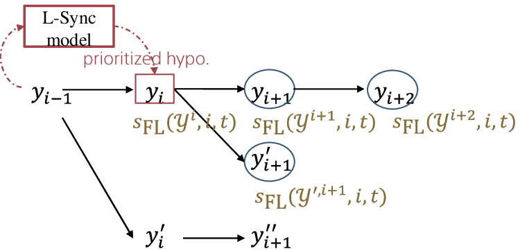
The priority of the hypothesis $\mathcal{Y}_{\mathrm{L}}^{i}$ is no longer valid once the L-Sync decoding increase its step $i\rightarrow i+1$, as it generate new set of hypotheses $\mathcal{Y}_{\mathrm{L}}^{i+1}$. Further, to prune unnecessary hypotheses of L-Sync decoding, we propose to perform ancestor-pruning, which is similar to the depth-pruning in [32]. As the F-Sync decoding proceed, it expands the hypothesis $\mathcal{Y}^{i}\rightarrow\mathcal{Y}^{i+1}$, as shown in Fig. 2. The prioritized root hypothesis $\mathcal{Y}^{i}$ is indicated by the red box and the expanded successors $\mathcal{Y}^{i+*}$ are indicated by the blue circles. We compare the scores of all the successors and the root hypothesis, denoted as $s_{\mathrm{FL}}$ in Fig. 2. When all the scores of successors become greater than the score of the root, $s_{\mathrm{FL}}(\mathcal{Y}_{\mathrm{L}}^{i},i,t)<\min(s_{\mathrm{FL}}(\mathcal{Y}^{i+*},i,t))$, we prune away prioritized root hypothesis $\mathcal{Y}_{\mathrm{L}}^{i}$, because any new successor from the root $\mathcal{Y}_{\mathrm{L}}^{i}$ can no longer achieve higher score than the current successors due to the $0\leq q(z_{t}|{\mathbf{h}}_{t},y_{i})\leq 1$ restriction.

The proposed beam search is summarized in Algorithm 1. As the FL-Sync decoding is performed based on the F-Sync frame-wise pruning, $t$ is increased at each step in the loop. First, L-Sync decoding is performed if step $i<\min(|Y\in\Omega_{\mathrm{FL},t-1}|)$ as descried in Sec. 3.1. The L-Sync decoding expands the prefixes of the hypotheses (Line 6) and provides prioritized hypotheses $\mathcal{Y}^{i}_{\mathrm{L}}$, which are maintained in temporary hypothesis set $\hat{\Omega}$ (Line 7). Then the F-Sync decoding is performed based on (10), and merged with the prioritized hypotheses (Line 9). Subsequently, in Line 10, the ancestor-pruning described in Sec. 3.3 is performed, which removes unnecessary hypotheses. The hypotheses from L-Sync decoding have priority for survival (Line 11), then lastly the hypothesis set is filled from the temporary set up to total beam size, $B^{\prime}$ (Line 12). Note that, even the total beam size increases from $B$ to $B^{\prime}$, computational impact is marginal from $B$-beam L-Sync decoding, because the F-Sync model, e.g., CTC, generally requires much less computation.

For the English evaluation, we trained a streaming encoder–decoder ASR model following [25] with the Librispeech dataset [34], a read speech corpus. It was applied to three various domains: The TED-LIUM 3 [35] dev/test set (a spontaneous lecture style), Hub5’00 (telephony-style conversation) having Switchboard (SWB) and CallHome (CHM) subsets, and voice-command-style STOP dataset [36].

For Japanese, we trained a streaming ASR model with a merged set of the lecture style CSJ [37] and LaboroTV corpus of TV program [38]. We used three evaluation sets of the CSJ dataset for intra-domain setup, and TEDxJP [38] for cross-domain setup. To cover various range of domains, We also used in-house evaluation data; 720 read news utterances (News) spoken by four males and four females, 2,620 voice commands (CMD1) and far-field 1,768 commands (CMD2), each spoken by 10 hired speakers.

The input acoustic features were 80-dimensional filter bank features. The input features were applied mean normalization with a sliding window. The encoder consisted of 12 blocks of conformer [6]. The AttDec had six decoder blocks. Each block consisted of four-head 256-unit attention layers and 2048-unit feed-forward layers. Contextual block encoding [22] was applied to the encoder with a block size of 40, a shift size of 16, and a look-ahead size of 16. The models were trained using multitask learning with CTC loss [33], with a weight of 0.3.

For English evaluation, external LMs were trained using each target dataset for adaptation. LMs were four-layer unidirectional LSTM with 2048 units, using the byte-pair encoding (BPE) subword tokenization with 5000 token classes. For Japanese, we collected over 27 million sentences to train a general LM with 10,000 BPE tokens, applied to all the tasks.

We compared our proposed FL-Sync decoding with streaming L-Sync decoding [25], and CTC F-Sync decoding [32]. We also evaluated AttDec score fusion for CTC F-Sync decoding for comparison. For the CTC F-Sync decoding methods, $\lambda_{\mathrm{lm}}=0.4$ was used for English datasets, and $\lambda_{\mathrm{lm}}=0.1$ for Japanese, instead. For the baseline L-Sync decoding and the proposed FL-Sync decoding, we adopted $(\lambda_{\mathrm{lm}},\lambda_{\mathrm{ctc}})=(0.4,0.4)$ for English intra-domain, $(0.6,0.4)$ for English cross-domain, and $(0.3,0.5)$ for Japanese experiments. $\lambda_{\mathrm{att}}$ was set as $(1-\lambda_{\mathrm{ctc}})$. We adopted $\lambda_{\mathrm{len}}=1$ for all the evaluation. We used $B^{\prime}=10$ and $B=5$ as a beam size for total FL-Sync decoding and L-Sync decoding in it, respectively. For fair comparison, we used the same beam sizes for the baseline approaches.

The word error rate (WER) results are summarized in Table 1. Streaming L-Sync decoding was generally better than CTC F-Sync decoding, particularly in the voice-command STOP dataset. This indicated that it is more effective in pruning to use input information including future look-ahead frames. Although the AttDec score fusion improved accuracy on CTC F-Sync decoding, the proposed FL-Sync decoding showed large improvement from those F-Sync decoding methods because it also preserved hypotheses from the L-Sync decoding. When we compare FL-Sync decoding with the L-Sync baseline decoding, our proposed method performed robustly in the cross-domain scenarios; for instance, WER was improved from 13.1% to 12.7% in TEDLIUM3 test set. Furthermore, we confirmed that it did not degrade the intra-domain performance, or even observed slight improvement from 8.1% to 7.9% in test-other, for instance. Since the scores, (7), (8), and (10), eventually become the same in all the search methods, the results show that our method is effective in pruning because of maintaining hypotheses from both L-Sync and F-Sync decoding.

We evaluated character error rates (CERs), which are listed in Table 2. The results followed similar tendency to the English evaluation. As we used the general LM, it did not exactly match to some of the target domains. As a result, we observed that even in the source domain CSJ eval sets, CERs were relatively higher than the other literature [25, 39]. Furthermore, the baseline L-Sync decoding had difficulty in adapting to the target domains, in particular in CMD2 data, which tend not to be grammatically structured. Since our proposed FL-Sync decoding maintained both L-Sync and F-Sync decoding, it recovered the domain bias and was robust to the cross-domain situation.

References

- [1] Alex Graves, Santiago Fernández, Faustino Gomez and Jürgen Schmidhuber “Connectionist temporal classification: labelling unsegmented sequence data with recurrent neural networks” In Proc. ICML, 2006, pp. 369–376
- [2] Alex Graves and Navdeep Jaitly “Towards end-to-end speech recognition with recurrent neural networks” In Proc. ICML, 2014, pp. 1764–1772
- [3] Yajie Miao, Mohammad Gowayyed and Florian Metze “EESEN: End-to-end speech recognition using deep RNN models and WFST-based decoding” In Proc. of ASRU Workshop, 2015, pp. 167–174
- [4] Dario Amodei “Deep Speech 2: End-to-End Speech Recognition in English and Mandarin” In Proc. ICML 48, 2016, pp. 173–182
- [5] Alex Graves, Abdel-Rahman Mohamed and Geoffrey Hinton “Speech recognition with deep recurrent neural networks” In Proc. ICASSP, 2013, pp. 6645–6649
- [6] Anmol Gulati, James Qin, Chung-Cheng Chiu, Niki Parmar, Yu Zhang, Jiahui Yu, Wei Han, Shibo Wang, Zhengdong Zhang and Yonghui Wu “Conformer: Convolution-augmented Transformer for Speech Recognition” In Proc. Interspeech, 2020, pp. 5036–5040
- [7] Qian Zhang, Han Lu, Hasim Sak, Anshuman Tripathi, Erik McDermott, Stephen Koo and Shankar Kumar “Transformer transducer: A streamable speech recognition model with transformer encoders and RNN-T loss” In Proc. ICASSP, 2020, pp. 7829–7833
- [8] Linhao Dong, Feng Wang and Bo Xu “Self-Attention Aligner: A Latency-Control End-to-End Model for ASR Using Self-Attention Network and Chunk-Hopping” In Proc. ICASSP, 2019, pp. 5656–5660
- [9] Jiahui Yu, Chung-Cheng Chiu, Bo Li, Shuo-yiin Chang, Tara Sainath, Yanzhang He, Arun Narayanan, Wei Han, Anmol Gulati and Yonghui Wu “FastEmit: Low-latency streaming ASR with sequence-level emission regularization” In Proc. ICASSP, 2021, pp. 6004–6008
- [10] Yangyang Shi, Yongqiang Wang, Chunyang Wu, Ching-Feng Yeh, Julian Chan, Frank Zhang, Duc Le and Mike Seltzer “Emformer: Efficient memory transformer based acoustic model for low latency streaming speech recognition” In Proc. ICASSP, 2021, pp. 6783–6787
- [11] Jan. Chorowski, Dzmitry Bahdanau, Dmitriy Serdyuk, Kyunghyun Cho and Yoshua Bengio “Attention-based models for speech recognition” In Proc. of NIPS, 2015, pp. 577–585
- [12] William Chan, Navdeep Jaitly, Quoc Le and Oriol Vinyals “Listen, attend and spell: A neural network for large vocabulary conversational speech recognition” In Proc. ICASSP, 2016, pp. 4960–4964
- [13] Tomas Mikolov, Martin Karafiát, Lukas Burget, Jan Cernockỳ and Sanjeev Khudanpur “Recurrent Neural Network Based Language Model” In Proc. Interspeech, 2010, pp. 1045–1048
- [14] Kazuki Irie, Albert Zeyer, Ralf Schlüter and Hermann Ney “Language modeling with deep transformers” In Proc. Interspeech, 2019, pp. 3905–3909
- [15] Jan Chorowski and Navdeep Jaitly “Towards Better Decoding and Language Model Integration in Sequence to Sequence Models” In Proc. Interspeech, 2017, pp. 523–527
- [16] Anjuli Kannan, Yonghui Wu, Patrick Nguyen, Tara Sainath, Zhijeng Chen and Rohit Prabhavalkar “An analysis of incorporating an external language model into a sequence-to-sequence model” In Proc. ICASSP, 2018, pp. 1–5828
- [17] Tara Sainath, Ruoming Pang, David Rybach, Yanzhang He, Rohit Prabhavalkar, Wei Li, Mirkó Visontai, Qiao Liang, Trevor Strohman and Yonghui Wu “Two-pass end-to-end speech recognition” In Proc. Interspeech, 2019, pp. 2773–2777
- [18] Wei Zhou, Simon Berger, Ralf Schlüter and Hermann Ney “Phoneme based neural transducer for large vocabulary speech recognition” In Proc. ICASSP, 2021, pp. 5644–5648
- [19] John Lafferty, Andrew McCallum and Fernando Pereira “Conditional random fields: Probabilistic models for segmenting and labeling sequence data” In Proc. ICML, 2001, pp. 282–289
- [20] Samy Bengio, Oriol Vinyals, Navdeep Jaitly and Noam Shazeer “Scheduled Sampling for Sequence Prediction with Recurrent Neural Networks” In Proc. NeurIPS 28, 2015
- [21] Kenton Murray and David Chiang “Correcting length bias in neural machine translation” In arXiv preprint arXiv:1808.10006, 2018
- [22] Emiru Tsunoo, Yosuke Kashiwagi, Toshiyuki Kumakura and Shinji Watanabe “Transformer ASR with Contextual Block Processing” In Proc. of ASRU Workshop, 2019, pp. 427–433
- [23] Niko Moritz, Takaaki Hori and Jonathan Le “Triggered Attention for End-to-end Speech Recognition” In Proc. ICASSP, 2019, pp. 5666–5670
- [24] Mohan Li, Cătălin Zorilă and Rama Doddipatla “Head-Synchronous Decoding for Transformer-Based Streaming ASR” In Proc. ICASSP, 2021, pp. 5909–5913
- [25] Emiru Tsunoo, Chaitanya Narisetty, Michael Hentschel, Yosuke Kashiwagi and Shinji Watanabe “Run-and-Back Stitch Search: Novel Block Synchronous Decoding For Streaming Encoder-Decoder ASR” In Proc. ICASSP, 2022, pp. 8287–8291
- [26] Qiujia Li, Chao Zhang and Philip Woodland “Combining frame-synchronous and label-synchronous systems for speech recognition” In arXiv preprint arXiv:2107.00764, 2021
- [27] Brian Yan, Siddharth Dalmia, Yosuke Higuchi, Graham Neubig, Florian Metze, Alan Black and Shinji Watanabe “CTC alignments improve autoregressive translation” In arXiv preprint arXiv:2210.05200, 2022
- [28] Linhao Dong, Cheng Yi, Jianzong Wang, Shiyu Zhou, Shuang Xu, Xueli Jia and Bo Xu “A comparison of label-synchronous and frame-synchronous end-to-end models for speech recognition” In arXiv preprint arXiv:2005.10113, 2020
- [29] Wei Zhou, Albert Zeyer, André Merboldt, Ralf Schlüter and Hermann Ney “Equivalence of segmental and neural transducer modeling: A proof of concept” In Proc. Interspeech, 2021, pp. 2891–2895
- [30] Emiru Tsunoo, Yosuke Kashiwagi and Shinji Watanabe “Streaming Transformer ASR With Blockwise Synchronous Beam Search” In Proc. SLT, 2021, pp. 22–29
- [31] Awni Hannun, Carl Case, Jared Casper, Bryan Catanzaro, Greg Diamos, Erich Elsen, Ryan Prenger, Sanjeev Satheesh, Shubho Sengupta and Adam Coates “Deep speech: Scaling up end-to-end speech recognition” In arXiv preprint arXiv:1412.5567, 2014
- [32] Kyuyeon Hwang and Wonyong Sung “Character-level incremental speech recognition with recurrent neural networks” In Proc. ICASSP, 2016, pp. 5335–5339
- [33] Shinji Watanabe, Takaaki Hori, Suyoun Kim, John. Hershey and Tomoki Hayashi “Hybrid CTC/attention architecture for end-to-end speech recognition” In Journal of Selected Topics in Signal Processing 11.8, 2017, pp. 1240–1253
- [34] Vassil Panayotov, Guoguo Chen, Daniel Povey and Sanjeev Khudanpur “LibriSpeech: an ASR corpus based on public domain audio books” In Proc. ICASSP, 2015, pp. 5206–5210
- [35] François Hernandez, Vincent Nguyen, Sahar Ghannay, Natalia Tomashenko and Yannick Esteve “TED-LIUM 3: twice as much data and corpus repartition for experiments on speaker adaptation” In International conference on speech and computer, 2018, pp. 198–208
- [36] Paden Tomasello, Akshat Shrivastava, Daniel Lazar, Po-Chun Hsu, Duc Le, Adithya Sagar, Ali Elkahky, Jade Copet, Wei-Ning Hsu and Yossi Adi “STOP: A dataset for spoken task oriented semantic parsing” In Proc. SLT, 2023, pp. 991–998
- [37] Kikuo Maekawa, Hanae Koiso, Sadaoki Furui and Hitoshi Isahara “Spontaneous Speech Corpus of Japanese” In Proc. of the International Conference on Language Resources and Evaluation (LREC), 2000, pp. 947–9520
- [38] Shintaro Ando and Hiromasa Fujihara “Construction of a large-scale Japanese ASR corpus on TV recordings” In Proc. ICASSP, 2021, pp. 6948–6952
- [39] Shigeki Karita, Yotaro Kubo, Michiel Bacchiani and Llion Jones “A comparative study on neural architectures and training methods for Japanese speech recognition” In Proc. Interspeech, 2021, pp. 2092–2096