ExWarp: Extrapolation and Warping-based Temporal Supersampling for High-frequency Displays
Abstract
High-frequency displays are gaining immense popularity because of their increasing use in video games and virtual reality applications. However, the issue is that the underlying GPUs cannot continuously generate frames at this high rate – this results in a less smooth and responsive experience. Furthermore, if the frame rate is not synchronized with the refresh rate, the user may experience screen tearing and stuttering. Previous works propose increasing the frame rate to provide a smooth experience on modern displays by predicting new frames based on past or future frames. Interpolation and extrapolation are two widely used algorithms that predict new frames. Interpolation requires waiting for the future frame to make a prediction, which adds additional latency. On the other hand, extrapolation provides a better quality of experience because it relies solely on past frames – it does not incur any additional latency. The simplest method to extrapolate a frame is to warp the previous frame using motion vectors; however, the warped frame may contain improperly rendered visual artifacts due to dynamic objects – this makes it very challenging to design such a scheme. Past work has used DNNs to get good accuracy, however, these approaches are slow. This paper proposes ExWarp– an approach based on reinforcement learning (RL) to intelligently choose between the slower DNN-based extrapolation and faster warping-based methods to increase the frame rate by 4 with an almost negligible reduction in the perceived image quality.
Index Terms:
Extrapolation, super-sampling, frame rateI Introduction
The CAGR (compound annual growth rate) for the global gaming market is projected to be 7.7% over the next 5 years [13]. This will lead to a total revenue of roughly 532.97 billion USD by 2027 [12]. To provide as realistic an experience as possible, displays are supporting increasingly higher refresh rates. We have moved from 30 Hz to 120 Hz over the last few years. Such systems help players feel fully involved in the virtual world. Given that the human vision system is exceptionally sensitive and can sometimes detect a lag as low as 2 ms [31], gamers prefer ultra-high refresh rates. For newer head-mounted displays, latencies greater than 7 ms may result in motion sickness and dizziness [37]. Even for non-gamers, research has shown that an inter-frame duration of 25 ms [27, 25] can cause issues. They will perceive a high latency in interactive tasks. The only solution is to render and display frames as fast as possible.
To meet these latency requirements, display vendors have launched monitors with high refresh rates such as 120 Hz, 240 Hz and 360 Hz displays [2, 1]. Recently, Dell launched the Alienware 500Hz Gaming Monitor. Mobile companies are also incorporating such displays into their devices. [9]. Similarly, there are GPUs such as the NVIDIA RTX series GPUs, which can render up to 360 frames per second at 1080p resolution [5]. Still users are not guaranteed to have a seamless experience because the actual frame rate depends upon various parameters such as the frame resolution, frame complexity, etc., and it varies a lot during the application Furthermore, if the frame rate is not synchronized with the refresh rate of the monitor, the user may experience glitches known as screen tearing and screen stuttering [18]. That is why there exist synchronization algorithms such as G-Sync and Free-Sync [34] in NVIDIA GPUs that modulate the refresh rate to synchronize it with the frame rate and prevent screen tearing and screen stuttering. However, this is not an ideal solution. Let us assume we have a 144 Hz monitor but the GPU is only supplying frames at 45 fps, then these synchronization techniques reduce the refresh rate to 45 Hz, which results in an ineffective use of the monitor’s capabilities. Hence, this work aims to temporally supersample the frames for enabling the use of high refresh rate displays.
Recent works propose two ways to increase the frame rate: spatial supersampling [22, 30, 40] and temporal supersampling [14, 16, 20, 41]. These works exploit the fact that with the increase in image resolution, there exists a similarity between neighboring pixels in spatial and temporal domains known as spatial and temporal coherence [22]. Spatial supersampling increases the frame rate by rendering the frames at a much lower resolution and then increases the resolution of the rendered frame before displaying them using interpolation. On the other hand, temporal supersampling generates entirely new frames on the fly using an already rendered frame. For temporal supersampling, there are two popular methods: Interpolation and Extrapolation [20]. Most of the existing works including NVIDIA’s latest supersampling method, DLSS 3 (Deep Learning SuperSampling) [17], use optical flow-based interpolation to generate new frames. The problem with the interpolation method is that one needs to wait till the next frame is rendered to start the interpolation (figure out all frames in between). This introduces an unnecessary delay leading to an increased input latency (refer to Section II-A1), which degrades the overall performance. The advantage of these methods is that they cover occlusion and disocclusion steps.
ExtraNet [20], an extrapolation method for temporal supersampling, proposes a
way that does not rely on optical flow and extrapolates the new frame solely based on the past few frames. To handle
occlusion and dynamic objects, ExtraNet uses a few intermediate buffers that are generated during the rendering
process. It relies on a complex neural network to do this task; hence it is slow. Due to its significant latency, it
upsamples the frame rate only by 1.5 to 2. This work proposes ExWarp– a faster extrapolation-based method to upsample
the frame rate further for high-frequency displays: from 30 to 120 Hz. Our primary contributions are:
We show that two
widely used methods used for predicting frames – warping and extrapolation – can be combined for temporal supersampling in
real-time.
We identify a few features that define the current state of the scene, i.e., the presence of
dynamic objects and camera movement.
We propose a reinforcement learning (RL) based approach that uses
these identified features to intelligently choose between extrapolation and warping based methods to increase the frame rate
by almost 4 with an almost negligible reduction in the perceived image quality.
We are able to
supersample the frame rate by nearly 4. We record an 18.02% increase in the PSNR and a 6.58% increase in SSIM
as compared to the state-of-the-art baseline, ExtraNet.
The paper is organized as follows. Section II provides the background of VR architectures and ML-based models. Section III shows the characterization of benchmarks. The implementation details are given in Section IV. Section V shows the experimental results. We discuss related work in Section VI and finally conclude in Section VII.
II Background
II-A Temporal Supersampling
As mentioned in Section I, temporal super-sampling relies on the fact that most of the content remains the same from frame to frame. A significant portion of a frame corresponds to at least a portion of either the previous, future, or both the frames [11]. This correspondence can be find out using optical flow vectors that describe the velocities of pixels within a frame [21].
II-A1 Interpolation Vs Extrapolation
As the name suggests, interpolation predicts a frame in between two already rendered neighboring frames. Whereas, extrapolation predicts frames based on the past frame(s) without considering future frame(s). Figure 1 explains these two algorithms in detail. In the figure, we observe that both interpolation and extrapolation introduce some latency in the system, which is their own operational latency. Both processes double the frame rate by generating a new frame after each rendered frame and display the frame in the following order . However, interpolation introduces an additional latency. Let us consider the newly generated frame with suffix . In interpolation, the frame is generated using two frames and . Since frame needs to be displayed before , it waits for , holds it, starts interpolating , and first displays the interpolated frame, and then . Hence, the input latency becomes interpolation cost + the time before displaying . Whereas in the case of extrapolation, the new frame, is generated only based on the past frame and all the frames are displayed at the very next refresh cycle.
II-B Image Warping
Image warping is a reprojection technique that maps all locations in one image to locations in a second image. It can be used to distort the original image in a way that serves a certain purpose. It can be used to perform various tasks such as correcting image distortion as well as for creative purposes like morphing [15]. One such task is frame prediction by warping the current frame to predict a future frame [32]. The accuracy of using warping on frame prediction depends on how well we understand the motion between the two frames. Most modern approaches use machine learning and Deep Neural Networks (DNNs) to estimate this motion [24] [20].
II-C Reinforcement Learning
Reinforcement Learning (RL) [38] is a machine learning-based technique that uses information about the environment and the feedback from its actions to learn an action inside the environment. It has been derived from reinforcement theory [28], which argues that human behavior is a direct result of the consequences of one’s actions. In machine learning, this technique generally doesn’t require any labeled data but requires the problem to be formulated as an actor in an environment defined by a tuple of the state space, action space, and associated rewards. The state space defines all the legal states for the actor to be in; however, note that most RL problems operating using incomplete information – the state space does not capture all aspects of the environment completely . The action space is the collection of all the actions that the actor is allowed to take in a state. The rewards are the gains/loss associated with each action in a particular state.
III Characterization
In this section, we first show the workloads used for experiments and the platform configuration for running experiments. As mentioned in Section II-A1, interpolation adds latency to the system in addition to its inherent operating latency, hence extrapolation is a preferable choice for temporal supersampling in real-time rendering systems. However, even extrapolation has some latency. So, in this section, we show the latency of the various steps involved in the extrapolation process used in ExtraNet. This is to find the reasons for its unacceptably large latency and possible solutions.
III-A Dataset
Similar to prior work [20], we use five different applications from the Unreal Engine marketplace [7] with different artistic backgrounds and different levels of complexities I. Together they cover a range of different shading effects and transforms. Each application has scenes with dynamically moving objects and different inter-frame variations. The experiments are run on an NVIDIA RTX series GPU. The detailed configuration is given in Table II.
| Abbr. | Name | Resolution | API | Platform |
| LB | Lab [8] | 480p | DX12 | UE |
| TR | Tropical [6] | 480p | DX12 | UE |
| VL | Village [4] | 480p | DX12 | UE |
| TN | Town [3] | 480p | DX12 | UE |
| TN2 | 720p | |||
| TN3 | 1080p | |||
| SL | Slum [10] | 480p | DX12 | UE |
| SL2 | 720p | DX12 | ||
| SL3 | 1080p | DX12 | ||
| UE: Unreal Engine, DX: DirectX | ||||
| Parameter | Type/Value |
|---|---|
| CPU | Intel®Xeon®Gold 6226R @ 2.90GHz |
| GPU | NVIDIA RTX™A4000 |
| GPU memory | 16 GB |
III-B Extrapolation Latency
To the best of our knowledge, there is only one prominent state-of-the-art work that uses extrapolation for temporal supersampling in real-time namely ExtraNet[20]. We consider ExtraNet as the baseline for our work. ExtraNet is a DNN-based approach to extrapolate frames. The authors of this work divide the extrapolation task into two stages. First, they simply warp the past frame and then feed the warped frame to the proposed neural network to synthesize the final frame. According to them, the warped frame created using only past frames may have some visible artifacts such as improper shadows and ghosting effects if there are dynamic objects or there is a movement in the camera. To remove these artifacts, they first mark invalid pixels in the warped frame and then use extrapolation to correct those pixels with the help of the neural network. The neural network takes the last three frames into account to capture more information about the scene. To mark invalid pixels as holes, they use a few intermediate buffers that are created during the rendering process, also known as geometry buffers or G-buffers. The input to the neural network is the warped frame based on the last three rendered frames, the corresponding images marked with holes and G-buffers.
Hence, the steps involved in the extrapolation process are G-buffer generation, image warping, hole marking and DNN-based inference for extrapolation. We measure the latency of each step separately for each application at different resolutions. The results are shown in Table III. These results are collected for 1000 frames per benchmark. We make the following observations from the table:
The latency of all the steps except G-buffer generation is almost constant across applications for a given
resolution because it depends upon the size of the input frames. Also, the latency increases with an increase in the
resolution or image size. The latency of G-buffer generation varies across applications because it depends upon the
scene complexity.
For all applications, the most time-consuming step is the inference part (latency: 3.5 ms to 13.8 ms), which puts a limit on the number of frames that can be extrapolated before the actual rendered frame. Hence, we propose to perform the inference or extrapolation only when it is necessary. We, instead, replace it with warping, which is faster (max latency: 4.6 ms) at the cost of accuracy.
| App. | G-buffer | Warping | Hole | Network |
| generation | marking | inference | ||
| LB | 0.17 | 0.95 | 1.94 | 3.67 |
| TR | 0.36 | 0.89 | 1.89 | 3.78 |
| VL | 0.48 | 0.83 | 1.81 | 3.45 |
| TN | 0.34 | 0.96 | 1.89 | 3.61 |
| TN2 | 1.01 | 1.58 | 2.49 | 7.04 |
| TN3 | 1.02 | 2.89 | 4.57 | 13.54 |
| SL | 0.24 | 0.95 | 1.93 | 3.55 |
| SL2 | 1.24 | 1.67 | 2.59 | 7.09 |
| SL3 | 2.1 | 2.91 | 4.63 | 13.78 |
III-C Holes in Warped Frames
In the previous section, we discussed that ExtraNet finds invalid pixels or holes in the warped frame and then uses a neural network to fill those holes. To see whether we can skip this hole-filling process and display the warped image itself on the display or if this hole-filling is indeed necessary, we plot the number of holes present in warped frames across benchmarks. We use 1000 frames for each benchmark to plot the results. The results are shown in Figure 2.
We make the following observations from the figure:
The number of invalid pixels in the warped frame depends on the scenes getting rendered. There may also be
frames with no holes.
For example, in the case of LB, almost 90% of full frames have less than 10%
invalid pixels, whereas, for TR, more than 60% of total frames have more than 20% invalid pixels.
This clearly shows that warping may provide better quality for some frames or many frames depending on the
type of application. Warping is clearly a much faster process.
This insight motivates us to propose a method to
choose between warping and extrapolation based on the state of the current scene.
III-D State Representation
As mentioned in Section III-C, there may or may not be holes in the warped frame. If there are holes in the frame, it means that there are dynamic objects or the camera is moving [20]. According to Scherzer et al. [36], the next frame may be predicted given the previously rendered frame and motion vectors only using warping if there are no dynamic objects in the scene. Therefore, we propose a method, a decision predictor, that chooses between the two alternatives: warping and extrapolation. Since the performance of these two methods depends on the scene’s type or current state, we must discover a way to determine the scene’s state before designing the predictor, i.e., whether there is any movement (beyond a threshold) in the objects or camera leading to holes in the warped frame. Once we know the state, we can choose between extrapolation and warping using the state information. Unlike ExtraNet, we do not require the precise location of the holes in this particular scenario. We wish to determine whether the current state may result in invalid pixels in the warped frame. Since we intend to produce frames for high-frequency displays, we need to find this information quickly. Therefore, we propose a few features that capture motion information and represent the system’s current state. We use a few auxiliary buffers used in the rendering process for this purpose.
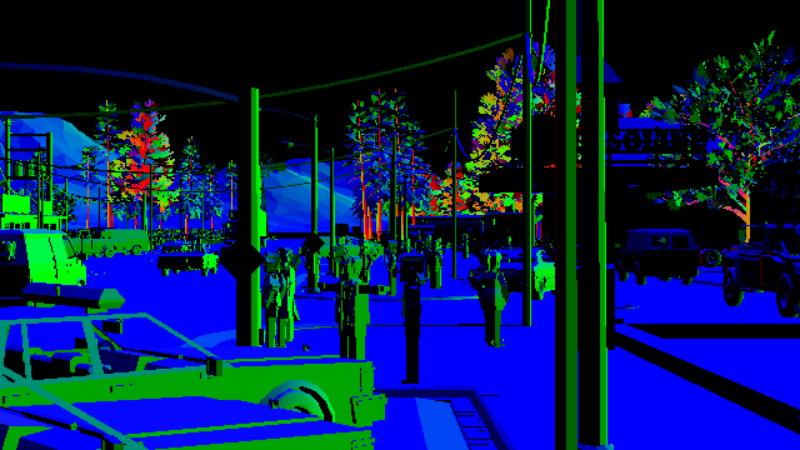
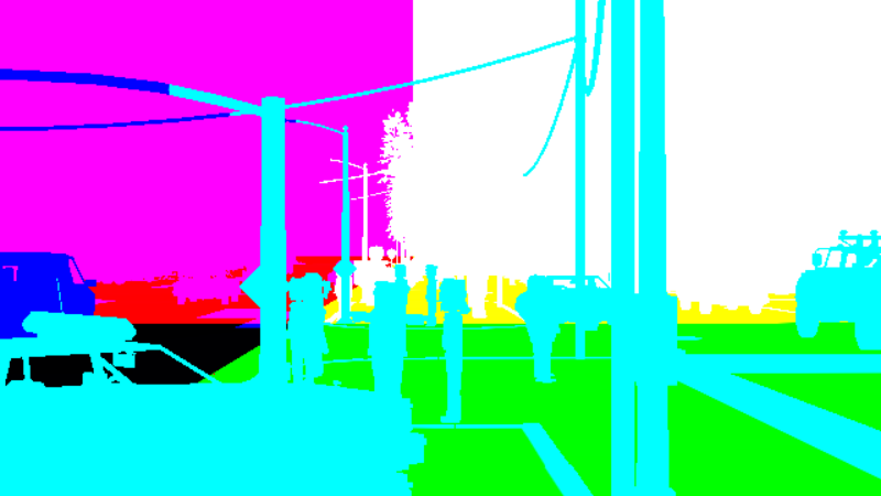
First, to capture dynamic objects, we use a motion vector buffer. A motion vector stores the motion information – direction and magnitude – of small blocks (areas of pixels) in the frame. Since the motion information in the block containing the dynamic object would differ from the background or static objects, we can use this for defining the state. We choose the variance in the motion as our feature. According to Guo et al. [20], three more buffers capture the dynamic movement information. Those are custom stencil, world position, and world normal (refer to Figure 3). As clearly shown in the figure, the custom stencil buffer directly captures dynamic objects. We use the clustering algorithm on the stencil buffer to find the number of dynamic objects present in the frame. Next, we have the world normal and world position buffers. The values change from the last frame to the current frame for these two buffers. We use a metric known as the Earth Movers Distance (EMD) [35] to capture the change in values for these buffers. The final list of features to define the current state is thus shown in Table IV.

| Feature | Description | Source buffer |
|---|---|---|
| Var | Variance in motion vector | Motion vector |
| EMD between buffers corresponding to and | World normal | |
| EMD between buffers corresponding to and | World position | |
| Number of dynamic objects | Custom stencil |
III-E Effect of the Identified Features
As mentioned in Section III-D, we use the identified features as inputs to the proposed predictor. We plot the
correlation between these variables and warping to demonstrate how they could help with the prediction. The results are
displayed in Figure 4. These results are for 1000 frames per benchmark.
Figure 4 shows the variation in the quality of the warped frame. The major insights from the results are as
follows:
The pattern for all the features is the same i.e., there is a decrease in the PSNR with increase
in the
features’ values.
We use this relation to design our model for the prediction.
IV Implementation
IV-A Overview
We propose to insert three new frames at time instances , , between any two consecutive frames and . As mentioned in Section I, warping and extrapolation are two options for synthesizing these new frames. Based on these two algorithms, multiple scenarios are possible (refer to Figure 5).
IV-B Problem Formulation
Given two rendered frames and , our goal is to insert new frames between these two frames without
using , where . We represent these frames as , where falls within the interval
and the frame is displayed on the screen at time . We have two options: warping and
extrapolation. For the ensuing discussion, please refer to
Figure 6. We need to make a decision about which frame to display – warped or extrapolated at three time
instants: , , . We refer to these frames as , , and ,
respectively.
Decision at : The decision () at this time decides which frame to display at : the warped version of () or the last displayed frame . The second choice would also result in the extrapolated () being displayed at . This is because the extrapolated frame would only be available at .
Decision at : The decision at this time instant decides which frame to display at . If the outcome of was to extrapolate, we do not need to take any decision at this point since we display at as explained above. If chose warping, then at this point we make decision , which chooses to display either the warped of the last displayed frame, i.e., or the extrapolated version of ().
Decision at : We decide which frame to display at . Depending on the outcomes of the previous two decisions, there are three possible cases. First, we consider the case where chose extrapolation. In this case, the decision decides whether to display the warped version of () or just display since extrapolation will not be able to generate the frame by . The other two cases are relevant if chose warping. For both of these cases, decisions and choose between the warped versions of () and extrapolated (). However, the frames and themselves would depend on the decision taken at . Based on these decisions, six scenarios or decision paths are possible (shown in Table V).
| Scenario | Frame rate | |||
| upsampling | ||||
| Extrapolated | Extrapolated | 2 | ||
| (ExtraNet) | (No new frame) | (No new frame) | ||
| Extrapolated | Warped | 3 | ||
| (No new frame) | ||||
| Warped | Extrapolated | Extrapolated | 4 | |
| Warped | Extrapolated | Warped | 4 | |
| Warped | Warped | Extrapolated | 4 | |
| Warped | Warped | Warped | 4 |
IV-C RL-based Decision Predictor
As mentioned in Section I, we propose an RL-based model II-C that intelligently takes the decisions shown in Figure 6 to provide the best overall performance both in terms of quality as well as frame rate. RL-based approaches are germane to this scenario because we take decisions in a potentially uncertain environment, and that too with partial information.
In this section, we define the structure, features, and parameters used in our network. As discussed in Section III-D, we feed the state information of the scenes to the model. The motivation behind the choice of values taken to represent the state has been summarized in Section III-E. To better understand the complexity of the current scene, we use the past three states with the current state as the input to make a prediction. Each state is defined by a tuple of vectors: the environment vector (Eqn. 1) and the temporal vector . The environment vector for any frame contains the values of the features mentioned in Table IV. We also consider the variance in the horizontal and vertical direction of the motion vector separately. We also use the rendering resolution () of as a single integer, (horiz vert).
| (1) |
To encode information about the current decision, we use another vector of length five, which represents the five states in Figure 6 as a one-hot encoded vector. The state is represented as . This tuple is flattened into a single vector and the concatenation of all the 4 state vectors (current and last three frames) are fed into the RL network. The length of the vector is 44 (114) 4-byte floats (represented in fixed point). The model gives an output vector of length two, which corresponds to the rewards associated with the two choices: warping and extrapolation. The choice that gives the maximum reward is chosen finally. Hence, the network is a mapping defined by . The predicted choice by the model at time () is calculated as:
| (2) |
To train our network to potentially foresee the future frames with high variation in features, we minimize the error between the predicted reward and the weighted sum of the current reward and the reward associated with the next best action. This ensures that the model is able to predict future high-variance sequences and take appropriate decisions. When the scene has less variation the model, we should prefer warping whereas when the scene is highly dynamic, the model needs to predict that and migrate towards extrapolation. It is important for our model to anticipate the future as the immediate best action might not be the best action (the local optima may not be global).
IV-C1 Reward Function
The reward function is the sum of the below at each decision point. Here, refers to the mean square error.
| (3) |
- •
- •
= -0.1, loss associated with dropping frames
The network estimates the reward function at state for an action with the network parameters at the training step. The function is the maximum reward in . Our loss can be defined as:
| (4) |
where (=0.95) is the discount factor, which is used to tune the importance the model gives to future moves and is the ground truth reward at that point.
Given that our input size is small, we can afford a network with three fully-connected+ReLU layers (, , , ) followed by one output layer (). Our network is trained with 3000 data points and tested with 1000 data points per benchmark. We generate the frames at 30 fps. We employ LOOCV cross-validation to prevent overfitting: test data points corresponding to one benchmark and use the remaining data points for training. We repeat this procedure for each benchmark (essentially, we rotate the train-test set) and report the mean.
IV-C2 Hardware Implementation of the Predictor
We train the predictor offline and use it for online inferencing. We implemented the predictor in Verilog and synthesized it. We used 4 simple cores in our design given its simplicity: each core has a four-stage pipelined architecture. Since, most of the operations in neural network inferencing are matrix multiplication and addition, we designed ten 8-bit multiply-accumulate (MAC) units along with one adder and one multiplier unit for each core. Each core has a private cache of 16 KB. The system architecture of the proposed system is shown in figure 7.
V Results and Analysis
V-A Performance Analysis
V-A1 Comparison of Various Possible Decision Paths
We showed the possible decision paths in Table V. In this section,
we compare the quality of the generated scenes.
The results are shown in
Table VI. We make the following observations from the results:
For most of the
benchmarks, ExWarp performs the best. Even if it is not the best, the values are comparable with the rest of the
methods.
There is an 18.02% and 6.58% increase in PSNR and SSIM in ExWarp, respectively, as compared to –
pure extrapolation-based method.
When compared to , a pure warping-based method, there is a 9.24%
and 0.04% increase in PSNR and SSIM, respectively.
| Scenes | Scenarios | ExWarp | ||||||
| PSNR(dB) | LB | 20.63 | 20.58 | 20.05 | 23.91 | 21.43 | 25.01 | 28.65 |
| TR | 19.82 | 19.18 | 19.11 | 22.60 | 20.19 | 23.68 | 17.30 | |
| VL | 20.33 | 19.92 | 24.90 | 36.36 | 32.68 | 43.70 | 44.66 | |
| TN | 18.29 | 17.56 | 16.94 | 19.71 | 19.97 | 17.39 | 24.10 | |
| TN2 | 18.70 | 16.85 | 15.60 | 17.98 | 17.35 | 15.06 | 17.12 | |
| TN3 | 19.26 | 17.14 | 15.64 | 17.91 | 16.98 | 14.79 | 17.01 | |
| SL | 29.06 | 28.86 | 30.11 | 31.38 | 32.10 | 30.93 | 32.62 | |
| SL2 | 31.17 | 29.20 | 28.20 | 29.97 | 26.83 | 27.59 | 32.33 | |
| SL3 | 30.99 | 29.40 | 27.83 | 28.52 | 26.43 | 26.90 | 32.03 | |
| SSIM | LB | 0.64 | 0.63 | 0.55 | 0.76 | 0.60 | 0.81 | 0.87 |
| TR | 0.63 | 0.59 | 0.51 | 0.69 | 0.54 | 0.71 | 0.55 | |
| VL | 0.80 | 0.77 | 0.69 | 0.92 | 0.75 | 0.99 | 0.99 | |
| TN | 0.75 | 0.73 | 0.64 | 0.78 | 0.79 | 0.65 | 0.81 | |
| TN2 | 0.78 | 0.71 | 0.61 | 0.70 | 0.66 | 0.56 | 0.69 | |
| TN3 | 0.82 | 0.74 | 0.62 | 0.72 | 0.66 | 0.57 | 0.71 | |
| SL | 0.88 | 0.87 | 0.77 | 0.92 | 0.94 | 0.78 | 0.93 | |
| SL2 | 0.88 | 0.85 | 0.72 | 0.88 | 0.71 | 0.87 | 0.87 | |
| SL3 | 0.88 | 0.86 | 0.72 | 0.87 | 0.72 | 0.87 | 0.87 | |
V-A2 Comparison with the State-of-the-Art
In this section, we compare the performance of our proposed model with two interpolation-based methods and ExtraNet. The interpolation-based methods are Softmax Splatting [33] and EMA-VFI [42]. All three methods are DNN-based techniques. Softmax splatting uses forward warping; it uses forward and backward motion flow (reprojection). However, in this approach, multiple pixels may map to the same target location in frame . Softmax splatting uses a modified softmax layer, which takes the frame’s depth data to handle this ambiguity. EMA-VFI uses a transformer network to perform frame interpolation. We show the performance of these methods in Table VII. For PSNR, ExWarp is the best for 4/9 benchmarks and the second best for two. There is a large difference only in the case of LB and TR. For the SSIM metric, both ExtraNet and ExWarp do well.
| Scenes | Interpolation | Extrapolation | |||
| EMA-VFI | Softmax Splatting | ExtraNet | ExWarp | ||
| PSNR(dB) | LB | 49.52 | 48.74 | 20.63 | 28.65 |
| TR | 24.60 | 23.42 | 19.82 | 17.30 | |
| VL | 20.86 | 20.54 | 20.33 | 44.66 | |
| TN | 14.40 | 13.84 | 18.29 | 24.11 | |
| TN2 | 13.42 | 13.47 | 18.70 | 17.12 | |
| TN3 | 14.15 | 14.53 | 19.27 | 17.01 | |
| SL | 28.57 | 24.07 | 29.06 | 32.62 | |
| SL2 | 24.58 | 22.74 | 31.16 | 32.33 | |
| SL3 | 32.53 | 34.95 | 30.99 | 32.03 | |
| SSIM | LB | 0.99 | 0.99 | 0.64 | 0.87 |
| TR | 0.97 | 0.95 | 0.63 | 0.55 | |
| VL | 0.94 | 0.93 | 0.80 | 0.99 | |
| TN | 0.82 | 0.77 | 0.75 | 0.81 | |
| TN2 | 0.71 | 0.59 | 0.78 | 0.69 | |
| TN3 | 0.75 | 0.64 | 0.82 | 0.71 | |
| SL | 0.61 | 0.26 | 0.88 | 0.93 | |
| SL2 | 0.40 | 0.27 | 0.88 | 0.87 | |
| SL3 | 0.75 | 0.83 | 0.88 | 0.87 | |
V-B Frame rate (FPS)
In this section, we plot the final frame rate achieved using ExWarp for each benchmark. As mentioned in
Section IV-C, the original frame rate was 30 fps. The results are shown in Figure 8. The insights from
the results are as follows:
The effective upsampled frame rate for all the benchmarks is more than 100 fps. We compute this based on the
number of new frames that we actually manage to insert. The more we extrapolate, lower is this figure.
The average frame rate across benchmarks is almost 110 fps, hence the supersampling factor is nearly 4 for
our proposed method. Note that this is more than all state-of-the-art work.
V-C Warping vs Extrapolation
Our proposed model, ExWarp, predicts the best method between warping and extrapolation. In this section, we plot the
prediction pattern of our predictor. The results are shown in Figure 9. The observations from the results
are as follows:
For most of the benchmarks, the ratio between warping and extrapolation is 80:20 except
VIL.
The average percentage for warping across benchmarks is 75.86%.
V-D Synthesis Results
We used the popular tool NNGen [39] to generate a baseline Verilog code for our neural network. We then made modifications to it and manually tuned it. We used the Cadence Genus Tool (TSMC 28 nm technology) to synthesize the design and obtain the power, area and timing numbers. Table VIII shows the area and power overheads of the hardware predictor. The total area is 0.12 , which is negligible. Also, the latency, 6.2 ns, is insignificant.
| Parameter | Value |
|---|---|
| Tool | Cadence Genus, 28 |
| Area | 0.12 |
| Power | 9.12 |
| Latency | 6.2 |
| Year | Work | Coherence Exploited | Method Used | ML-based | Upsampling |
|---|---|---|---|---|---|
| 2007 | Nehab et al. [30] | Spatial and temporal | Interpolation | ||
| 2010 | Andreev et al. [14] | Temporal | Interpolation | x to 60 fps | |
| 2010 | Didyk et al. [19] | Temporal | Interpolation | 40 fps to 120 fps | |
| 2010 | Herzog et al. [22] | Spatial and temporal | Interpolation | ||
| 2011 | Yang et al. [41] | Temporal | Interpolation | ||
| 2012 | Bowles et al. [16] | Temporal | Interpolation | ||
| 2018 | SAS [29] | Temporal | Interpolation | from (7.5,15,30, 60) fps to 120 fps | |
| 2021 | ExtraNet [20] | Temporal | Extrapolation | ✓ | upto 2 (30 fps to 60 fps) |
| 2022 | DLSS 3 [17] | Spatial and temporal | Interpolation | ✓ | upto 4 |
| 2023 | Our work | Temporal | Extrapolation | ✓ | upto 3 |
VI Related Work
Over the past few years, a variety of solutions have been developed that exploit the spatial and temporal coherence present in graphics applications to increase the frame rate of graphics applications and synchronize the GPU refresh rate with the display refresh rate for a seamless user experience. Recent works primarily focus on predicting new frames using interpolation [41, 30, 22, 14, 26] and generating new frames using extrapolation [20] to increase the frame rate. We present a brief comparison of related work in Table IX. The high processing cost per frame is the primary cause of the low frame rate [30], and previous works aim to decrease this cost. According to Herzog et al. [22], the visual appearance, illumination parameters, etc., are nearly identical between any two consecutive frames and sometimes within a single frame – they are known as temporal and spatial coherence, respectively. These effects can be exploited to reduce the overall processing cost per frame. They mention that although approaches based on reducing the resolution of a frame, predicting the next few frames, and then performing spatial supersampling are very efficient, such approaches can also undersample or blur sharp image features such as edges quite frequently. On the other hand, pure temporal supersampling is markedly better. This work is based on exclusive temporal supersampling.
VI-A Interpolation
Previous approaches [30] that use the temporal supersampling to fill in a frame between a pair of rendered frames use the interpolation process that is guided by the scene flow: the 3D velocities of visible surface points between two frames. For each pixel in an intermediate frame, the motion vector indicates where to pull pixel information from the original frames. Early approaches had a fundamental drawback, which was that whenever the scene contained regions that were visible in the current frame but were not in the previous one, the results were sub-par. Although Bowles et al. [16] proposed an efficient way to fix this using an iterative method called fixed point iteration (FPI), this did not provide satisfactory results. To handle this case, various works [41, 19, 17, 29] propose a bidirectional reprojection method that temporally upsamples rendered content by reusing data from both the backward and forward temporal directions. Didyk et al. [19] use motion flow to warp the previously shaded result into an in-between frame that is then locally blurred to hide artifacts caused by morphing failures. Finally, they compensate for the lost high-frequencies due to this blur by adding additional high frequencies wherever necessary. They perform an upsampling from 40 Hz to 120 Hz. Similarly, NVIDIA’s DLSS 3 [17] use the optical flow computed from both the backward and temporal directions to interpolate the frame. DLSS3 has two major components: an optical-flow generator and a frame generator apart from the supersampling network. They use the in-built accelerator in their latest GPU architecture Ada for the optical flow generation. The frame generator uses an AI-accelerated network that takes the computed optical flow to generate an entirely new frame. As shown in Figure 1, this approach increases the frame rate but also leads to an increased input latency that can easily be perceived by users. Since our approach is not based on optical flow fields, it does not require future frames to predict a new frame.
Nehab et al. [30] use a reverse reprojection-based caching technique to store the information that can be reused in the next frame, thereby avoiding the recomputation of the entire frame. Andreev et al. [14] propose an approach to maintain a consistent rate of 60 fps by dividing a frame into two parts: slow-moving and fast-moving, and rendering each one at a different rate (slower parts at a lower rate and faster parts at a higher rate). This approach works because some tests have shown that the temporal coherence of slowly moving parts is greater than that of other parts. Such approaches increase the time required for an application to construct a frame while maintaining a constant frame rate.
VI-B Extrapolation
VII Conclusion
With high-frequency displays becoming increasingly popular, it is now necessary to generate frames for real-time applications at higher rates. Since applications are very demanding in terms of processing power, it is not possible for even the most capable GPUs to constantly provide a high frame rate at an HD/4k resolution. It has become evident that new frames need to be generated without having to go through the entire graphics pipeline. This work illustrates one such method, ExWarp, of supersampling in the temporal domain, while maintaining frame quality. The existing methods use extrapolation to increase the frame rate but we observed that it is not always necessary to use an expensive method like extrapolation and that the decision to extrapolate or use a faster method such as warping can be intelligently made. We designed such a predictor to take this decision. We were able to achieve nearly four times the frame rate ( Hz) with a reasonably small reduction in the quality.
References
- [1] “360 Hz Monitors,” https://www.amazon.in/s?k=360+hz+monitor&i=computers&crid=1F5BQK6PBHFOW&sprefix=360+hz+monit%2Ccomputers%2C215&ref=nb_{}sb_{}noss_{}2, [Online; accessed 2023-05-08].
- [2] “360 Hz NVIDIA G-SYNC,” https://www.nvidia.com/en-in/geforce/technologies/360-hz/, [Online; accessed 2023-05-08].
- [3] “Assetsvilletown,” https://www.unrealengine.com/marketplace/en-US/product/assetsville-town, [Online; accessed 2023-05-20].
- [4] “Fantasticvillagepack,” https://www.unrealengine.com/marketplace/en-US/product/fantastic-village-pack, [Online; accessed 2023-05-20].
- [5] “Frames Win Games Lowest System Latency, Highest FPS,” https://www.nvidia.com/en-in/geforce/campaigns/frames-win-games/, [Online; accessed 2023-05-12].
- [6] “Lpsdeluxe2tropicalenvironment,” https://www.unrealengine.com/marketplace/en-US/product/low-poly-style-deluxe-2-tropical-environment, [Online; accessed 2023-05-20].
- [7] “Marketplace,” https://www.unrealengine.com/marketplace/en-US/store, [Online; accessed 2023-05-23].
- [8] “Modsciengineer,” https://www.unrealengine.com/marketplace/en-US/product/modular-scifi-engineer-interiors, [Online; accessed 2023-05-20].
- [9] “Smartphones with 120 Hz displays,” https://www.amazon.in/s?k=120hz+display+smartphones&crid=3LI5TROIGPD3D&sprefix=120hz+display+smartphones%2Caps%2C357&ref=nb_{}sb_{}noss_{}2, [Online; accessed 2023-05-19].
- [10] “Soulcity,” https://www.unrealengine.com/marketplace/en-US/product/soul-city, [Online; accessed 2023-05-20].
- [11] “Temporal supersampling and antialiasing,” https://bartwronski.com/2014/03/15/temporal-supersampling-and-antialiasing/, mar 15 2014, [Online; accessed 2023-05-08].
- [12] “Games,” https://www.statista.com/outlook/amo/media/games/worldwide, 2021, [Online; accessed 2023-05-08].
- [13] M. F. M. , “Gaming Industry vs. Other Entertainment Industries (2023),” https://raiseyourskillz.com/gaming-industry-vs-other-entertainment-industries-2021/, aug 9 2022, [Online; accessed 2023-05-08].
- [14] D. Andreev, “Real-time frame rate up-conversion for video games: or how to get from 30 to 60 fps for” free”,” in ACM SIGGRAPH 2010 Talks, 2010, pp. 1–1.
- [15] T. Beier and S. Neely, “Feature-based image metamorphosis,” ACM SIGGRAPH computer graphics, vol. 26, no. 2, pp. 35–42, 1992.
- [16] H. Bowles, K. Mitchell, R. W. Sumner, J. Moore, and M. Gross, “Iterative image warping,” in Computer graphics forum, vol. 31, no. 2pt1. Wiley Online Library, 2012, pp. 237–246.
- [17] A. Burnes and H. C Lin, “Nvidia DLSS 3: Ai-Powered Performance Multiplier Boosts Frame Rates By Up To 4x,” https://www.nvidia.com/en-us/geforce/news/dlss3-ai-powered-neural-graphics-innovations/, sep 20 2022, [Online; accessed 2023-05-09].
- [18] P. Davarmanesh, K. Jiang, T. Ou, A. Vysogorets, S. Ivashkevich, M. Kiehn, S. H. Joshi, and N. Malaya, “Automating artifact detection in video games,” arXiv preprint arXiv:2011.15103, 2020.
- [19] P. Didyk, E. Eisemann, T. Ritschel, K. Myszkowski, and H.-P. Seidel, “Perceptually-motivated real-time temporal upsampling of 3d content for high-refresh-rate displays,” in Computer Graphics Forum, vol. 29, no. 2. Wiley Online Library, 2010, pp. 713–722.
- [20] J. Guo, X. Fu, L. Lin, H. Ma, Y. Guo, S. Liu, and L.-Q. Yan, “Extranet: real-time extrapolated rendering for low-latency temporal supersampling,” ACM Transactions on Graphics (TOG), vol. 40, no. 6, pp. 1–16, 2021.
- [21] J. Heo and J. Jeong, “Forward warping-based video frame interpolation using a motion selective network,” Electronics, vol. 11, no. 16, 2022. [Online]. Available: https://www.mdpi.com/2079-9292/11/16/2553
- [22] R. Herzog, E. Eisemann, K. Myszkowski, and H.-P. Seidel, “Spatio-temporal upsampling on the gpu,” in Proceedings of the 2010 ACM SIGGRAPH symposium on Interactive 3D Graphics and Games, 2010, pp. 91–98.
- [23] A. Hore and D. Ziou, “Image quality metrics: Psnr vs. ssim,” in 2010 20th international conference on pattern recognition. IEEE, 2010, pp. 2366–2369.
- [24] X. Jin, L. Wu, G. Shen, Y. Chen, J. Chen, J. Koo, and C.-h. Hahm, “Enhanced bi-directional motion estimation for video frame interpolation,” in Proceedings of the IEEE/CVF Winter Conference on Applications of Computer Vision, 2023, pp. 5049–5057.
- [25] R. Jota, A. Ng, P. Dietz, and D. Wigdor, “How fast is fast enough? a study of the effects of latency in direct-touch pointing tasks,” in Proceedings of the sigchi conference on human factors in computing systems, 2013, pp. 2291–2300.
- [26] E. Liu, “Dlss 2.0 - image reconstruction for real-time rendering with deep learning,” in Game Developers Conference, 2020.
- [27] M. Long and C. Gutwin, “Effects of local latency on game pointing devices and game pointing tasks,” in Proceedings of the 2019 CHI Conference on Human Factors in Computing Systems, 2019, pp. 1–12.
- [28] F. Luthans and A. D. Stajkovic, “Reinforce for performance: The need to go beyond pay and even rewards,” Academy of Management Perspectives, vol. 13, no. 2, pp. 49–57, 1999.
- [29] J. H. Mueller, P. Voglreiter, M. Dokter, T. Neff, M. Makar, M. Steinberger, and D. Schmalstieg, “Shading atlas streaming,” ACM Transactions on Graphics (TOG), vol. 37, no. 6, pp. 1–16, 2018.
- [30] D. Nehab, P. V. Sander, J. Lawrence, N. Tatarchuk, and J. R. Isidoro, “Accelerating real-time shading with reverse reprojection caching,” in Graphics hardware, vol. 41, 2007, pp. 61–62.
- [31] A. Ng, J. Lepinski, D. Wigdor, S. Sanders, and P. Dietz, “Designing for low-latency direct-touch input,” in Proceedings of the 25th Annual ACM Symposium on User Interface Software and Technology, ser. UIST ’12. New York, NY, USA: Association for Computing Machinery, 2012, p. 453–464. [Online]. Available: https://doi.org/10.1145/2380116.2380174
- [32] S. Niklaus and F. Liu, “Softmax splatting for video frame interpolation,” in Proceedings of the IEEE/CVF Conference on Computer Vision and Pattern Recognition (CVPR), June 2020.
- [33] ——, “Softmax splatting for video frame interpolation,” in Proceedings of the IEEE/CVF Conference on Computer Vision and Pattern Recognition, 2020, pp. 5437–5446.
- [34] M. Riahi and B. A. Watson, “Am i playing better now? the effects of g-sync in 60hz gameplay,” Proceedings of the ACM on Computer Graphics and Interactive Techniques, vol. 4, no. 1, pp. 1–17, 2021.
- [35] Y. Rubner, C. Tomasi, and L. J. Guibas, “The earth mover’s distance as a metric for image retrieval,” International journal of computer vision, vol. 40, no. 2, p. 99, 2000.
- [36] D. Scherzer, M. Wimmer, E. Eisemann et al., “A survey on temporal coherence methods in real-time rendering,” 2011.
- [37] J.-P. Stauffert, F. Niebling, and M. E. Latoschik, “Latency and cybersickness: Impact, causes, and measures. a review,” Frontiers in Virtual Reality, vol. 1, p. 582204, 2020.
- [38] R. S. Sutton, A. G. Barto et al., “Reinforcement learning,” Journal of Cognitive Neuroscience, vol. 11, no. 1, pp. 126–134, 1999.
- [39] M. Tosini and G. Acosta, “Nngen: a powerful tool for the implementation of artificial neural networks on a chip,” Electronic Journal of SADIO (EJS), vol. 6, pp. 42–52, 2004.
- [40] L. Yang, P. V. Sander, and J. Lawrence, “Geometry-aware framebuffer level of detail,” in Computer Graphics Forum, vol. 27, no. 4. Wiley Online Library, 2008, pp. 1183–1188.
- [41] L. Yang, Y.-C. Tse, P. V. Sander, J. Lawrence, D. Nehab, H. Hoppe, and C. L. Wilkins, “Image-based bidirectional scene reprojection,” in Proceedings of the 2011 SIGGRAPH Asia Conference, 2011, pp. 1–10.
- [42] G. Zhang, Y. Zhu, H. Wang, Y. Chen, G. Wu, and L. Wang, “Extracting motion and appearance via inter-frame attention for efficient video frame interpolation,” 2023.
