Proximal Galerkin: A structure-preserving finite element method for pointwise bound constraints Thanks: Submitted to the editors August 11, 2026.
Abstract
The proximal Galerkin finite element method is a high-order, low iteration complexity, nonlinear numerical method that preserves the geometric and algebraic structure of pointwise bound constraints in infinite-dimensional function spaces. This paper introduces the proximal Galerkin method and applies it to solve free boundary problems, enforce discrete maximum principles, and develop a scalable, mesh-independent algorithm for optimal design with pointwise bound constraints. This paper also introduces the latent variable proximal point (LVPP) algorithm, from which the proximal Galerkin method derives.
When analyzing the classical obstacle problem, we discover that the underlying variational inequality can be replaced by a sequence of second-order partial differential equations (PDEs) that are readily discretized and solved with, e.g., the proximal Galerkin method. Throughout this work, we arrive at several contributions that may be of independent interest. These include (1) a semilinear PDE we refer to as the entropic Poisson equation; (2) an algebraic/geometric connection between high-order positivity-preserving discretizations and certain infinite-dimensional Lie groups; and (3) a gradient-based, bound-preserving algorithm for two-field, density-based topology optimization. The complete proximal Galerkin methodology combines ideas from nonlinear programming, functional analysis, tropical algebra, and differential geometry and can potentially lead to new synergies among these areas as well as within variational and numerical analysis. Open-source implementations of our methods accompany this work to facilitate reproduction and broader adoption.
keywords
Pointwise bound constraint, variational inequality, high-order finite element method, proximal point method, entropy regularization, bregman divergence, obstacle problem, discrete maximum principle, topology optimizationFunding.
BK was supported in part by the U.S. Department of Energy Office of Science, Early Career Research Program under Award Number DE-SC0024335. BK was also supported in part by the LLNL-LDRD Program under Project Tracking No. 22-ERD-009.Dedicated with respect and admiration to Leszek Demkowicz on the occasion of his 70th birthday.
AMS
35J86, 35R35, 49J40, 47J20, 49M41, 65K05, 65K10, 65K15, 65N30, 90C06, 90C251 Introduction
Although the origins of variational analysis can be traced back at least to the seventeenth century [167], its role in the modern study of partial differential equations (PDEs) only truly began to take shape around 1847 once William Thomson introduced what is now known as the Dirichlet principle. In contemporary language, this energy principle states that for all functions and , the (weak) solution of Poisson’s equation over a Lipschitz domain ,
| (1) |
can be obtained as the -minimizer of the Dirichlet energy,
| (2) |
confined to the constraint set .
Owing to the fact that is nonempty, closed, and convex, it is a consequence of the Lions–Stampacchia theorem [188, 141] that the energy minimizer is the unique solution to the variational inequality (VI)
| (3) |
It happens that the boundary condition in eq. 1 is an equality constraint that induces an affine structure on the feasible set. Moreover, it is this particular algebraic structure that can be exploited to show that the minimizer is also uniquely characterized by a variational equation. In the setting above, we have
| (4) |
To arrive at this conclusion from eq. 3, the key idea is to notice that and, therefore, one may replace in eq. 3 by , for any . For further details, see, e.g., [40, Proposition 9.22] and [50, Theorem 1.2.2].
A related additive structure appears if we consider imposing the pointwise non-negativity constraint, , and setting . Hereafter, let . In this setting, the feasible set
| (5) |
forms a closed convex cone in . It is well-known that the conic structure of allows us to write
| (6) |
with equality holding for ; see, e.g., [50, Theorem 1.1.2]. Thus, we encounter another simplification directly from the algebraic structure of the feasible set. This work pursues a third type of algebraic structure.
Our aim is to provide a high-order, multiplicative structure-preserving approach to solving bound-constrained optimization problems and variational inequalities in Sobolev spaces. This will lead us to working in Banach algebras, which are Banach spaces that are closed under a continuous multiplication operation [53]. Instead of performing Lagrangian relaxation or relying on penalty functions, the key component of our approach is an adaptive form of entropy regularization. Through entropy regularization, we will find, e.g., that minimizing the Dirichlet energy over functions in can be reduced to solving a sequence of second-order semilinear PDEs where each right-hand side is conditioned by the prior solution.
Algorithm 1 outlines the meta-algorithm for minimizing the Dirichlet energy under the pointwise non-negativity constraint considered above when and satisfies . Note that, unlike, e.g., descent methods [215, Section 3], this algorithm converges for all step size values ; cf. Theorem 17. A practical version of the algorithm appears via a saddle-point reformulation of the semilinear subproblem eq. 7, leading to the finite element method that gives this paper its name.
| (7) |
Remark 1 (Latent variable proximal point vs. proximal Galerkin).
Two general approximation techniques are introduced in this work: the latent variable proximal point (LVPP) algorithm and the proximal Galerkin finite element method. LVPP is an infinite-dimensional optimization algorithm, equivalent to a saddle-point reformulation of the (entropic) Bregman proximal point algorithm [198], which dates back to early work by Bregman, Nemirovskij, and Yudin [38, 164]. The proximal Galerkin finite element method is a nonlinear mixed method derived by discretizing the LVPP subproblems with the Galerkin finite element method. Although other numerical methods, e.g., finite difference, finite volume, spectral, spline, or even neural network methods could also be used to discretize LVPP, we focus our attention on the aforementioned finite element approach. We also acknowledge the existence of significantly different “proximal Galerkin” method proposed in [147], yet choose to use the same name for our method without any cause for confusion.
Remark 2 (Why pursue high-order discretizations?).
The solutions to variational inequality problems, as with other nonlinear problems, often have low regularity, potentially leading to low-order accuracy. In the early days of the finite element method, this fact led much of the community to conclude that low-order methods “are sufficient for all practical purposes” [50, Chapter 5]. Much to the contrary, high-order discretizations are now widely-used to solve nonlinear problems [209, 54] owing, in part, to more the accurate computational geometries [54] and higher efficiency on modern computing architectures; see, e.g., [17]. The benefits of high-order methods can be further improved when combined with adaptive mesh refinement, such as -refinement [185, 62]. This often (sometimes provably [206]) results in high-order accuracy, similar to if the underlying solution was smooth. These aspects all support the present investigation into a high-order methodology for discretizing variational inequalities.
1.1 Notation
Our notation is rather standard for the finite element literature. Norms are denoted by , inner products by , and duality pairings by for Banach spaces and its paired topological dual . Whenever it is clear in context, we leave off or abbreviate the subscripts in a natural way. For weak convergence, we use the standard notation, or . For subsets of infinite dimensional spaces, we denote the closure by , the boundary by , and the interior by . For a mapping between normed linear spaces and , the Fréchet derivative of at is indicated by .
For an open bounded domain , , , , denotes the usual Lebesgue space of (equivalence classes of) -integrable functions when , and essentially bounded functions when , respectively. Furthermore, we simplify the -inner product notation to and define
for any .
For domains in , we denote the boundary by and the closure by . The spaces are defined in the usual way. When needed, we indicate the surface measure for by . The space of continuous functions on is written . Similarly, , , is the space of all -times continuously differentiable functions. The space of smooth compactly supported test functions on is given by . The Sobolev space of functions with integrable weak derivatives is denoted by and its closed subspace of functions with trace is denoted by . We use , , for the usual Sobolev–Slobodeckij space on . We refer the reader to a standard text on function spaces for further details, e.g., [4, 155]. Finally, we adopt the following notational conventions: , , , and , with ignored in this and similar expressions.
1.2 Outline
We have attempted to provide a scaffolded presentation of our findings. To this end, Section 2 presents preliminary concepts and provides further motivation for this work. Next, Section 3 reviews the literature and summarizes our main contributions. Sections 4 through 6 present the essential features of proximal Galerkin methods for the obstacle problem, the advection-diffusion equation, and topology optimization, respectively. Each of these sections contains an algorithm that is designed be implemented in a production-level finite element code. The reader is encouraged to compare these algorithms with our publicly available implementations [112, 113, 114]. The main paper closes with Section 7, which contains a small number of concluding remarks, and then proceeds to two technical appendices. Appendix A contains the continuous-level mathematical analysis and Appendix B contains the discrete-level, finite element theory. Appendices A and B are the most specialized sections of the paper and may be skipped by a casual reader.
2 Preserving multiplicative structure
The proximal Galerkin finite element method is a nonlinear numerical method that preserves the algebraic and geometric structure of bound constraints in infinite-dimensional function spaces. It relies on reformulating subproblems like eq. 7 into a saddle-point form and discretizing the resulting system of equations. In this section, we outline the essential features of the method using Dirichlet energy minimization eq. 2 as a motivating example. First, however, we study the multiplicative structure of non-negative functions in order to illustrate how proximal Galerkin preserves this structure.
2.1 Deconstructing the semiring of non-negative functions
Here, we discuss the natural logarithmic transformation between non-negative functions and extended real-valued functions that may take the value . This also first introduces the latent variable . We claim this provides a basis for the use of logarithmic transformations to analyze and solve PDEs, an idea that goes back at least to work by Schrödinger in 1926. Finally, we address the somewhat unnatural conditions this transformation imposes on the solution spaces and variational equations themselves. In turn, we show how a simple regularization of the transformed equations remedies these concerns. We use this discussion to motivate the natural function spaces for pointwise bound constraints in and construct a direct link to entropy regularization.
Let be a set equipped with two binary operations: addition and multiplication .
Definition 3 (Semiring).
We say that is a semiring if the following conditions are satisfied [81, 83]:
- •
Addition and multiplication are associative;
- •
Addition is commutative;
- •
Multiplication is distributive with respect to addition .
We say that is a commutative semiring if the conditions above are satisfied and, moreover, multiplication is commutative.
It is easy to check that the set of non-negative Lebesgue measurable functions,
| (8) |
forms a commutative semiring under the standard binary operations of pointwise addition and multiplication. In particular, note that for any , we have
| (9) |
There is an interesting identification between and the space of extended real-valued measurable functions
| (10) |
induced by the (pointwise) logarithm and exponential operators. Namely, for all , , and , we have that and under the convention that and, likewise, . Such logarithmic transformations provide a family of semiring isomorphisms between and , where is endowed with the following (generalized) addition and multiplication operations:
| (11) |
respectively [152, 153]. Moreover, in the limit , the generalized addition operation eq. 11 becomes the pointwise maximum operation [143, 148]; namely,
| (12) |
Logarithmic transformations of the above form have been used famously over the last century to analyze differential equations in quantum mechanics [184], fluid flow [100, 52], and electrical engineering [180, 149], and, more recently, to study stochastic PDEs [30, 90]. Given that they appear to capture certain key algebraic properties of the set of non-negative functions, it is tempting to use logarithmic transformations to enforce non-negativity constraints on function spaces. Unfortunately, however, special care is required to apply a logarithmic transformation to a non-negative solution variable in a free-boundary problem.
For illustration, consider minimizing the Dirichlet energy eq. 2 over the set of non-negative functions
| (13) |
Assuming that and , the well-known complementarity conditions for the solution are as follows [117, p. 79]:
| (14) |
Another perspective uses a dual variable , also known as a Lagrange multiplier, to formulate eq. 14 as a mixed complementarity problem of the form:
| (15) |
The Lagrange multiplier exhibits rather low regularity for general domains , so the term “” is actually understood to mean for all with a.e. in , i.e., without further regularity assumptions is merely a nonnegative Radon measure on . See [117, Chap. II, Sec. 6] for details.
If we wish to study this problem under a logarithmic transformation, then a formal computation using the substitution leads to the observation that
| (16) |
at almost every point in . Analyzing these equations presents challenges, in part, because it requires moving away from well-studied Sobolev spaces [4] and, instead, working in a latent space of extended real-valued functions [118] endowed with the metric
| (17) |
More specifically, it is difficult to imagine how to rigorously discretize a space of functions that are allowed to take the value on sets of positive Lebesgue measure.
One conclusion of this work is that the above concerns are alleviated by a simple regularization of the degenerate PDE in eq. 16. In particular, we show that for all bounded , the latent solution variable is recovered as the limit (with respect to the metric eq. 17) of a family of regularized solutions satisfying
| (18) |
Moreover, the latent variable iteration ,
| (19) |
formerly written with primal variables in Algorithm 1, converges to for all finite ; cf. Theorem 17.
The ambient function space for the regularized latent variable is interesting from an algebraic point of view because it is a Banach algebra. Indeed, the Sobolev subspace , whose norm is
| (20) |
is closed under the standard operations of pointwise addition and multiplication [40, Proposition 9.4]. Maintaining closure under multiplication is desirable, in part, because it often allows one to construct a smooth exponential map [77, 78]. Indeed, of particular interest to this work is the Nemytskii operator
| (21) |
which is an isomorphism between and the Banach–Lie group
| (22) |
cf. Proposition 40. Since the range of this isomorphism is contained in the -interior of the set of essentially bounded non-negative functions, we find that the primal iterates,
will always be interior points. In the next motivational subsection, we explain that an identical sequence of interior points can be found by regularizing the Dirichlet energy with an appropriate entropy functional.
2.2 Dirichlet free energy
Only special function spaces are endowed with a norm topology that permits a continuous multiplication operator. Indeed, it is well-known that is only closed under multiplication when [4]. Moreover, it is easy to show that for all , which makes it impossible to define an -interior point in any of its subsets (cf. Remark 7). Because bypasses both of these topological issues, it is appealing to restrict the feasible set in eq. 13 to essentially bounded functions when minimizing the Dirichlet energy.
Unfortunately, requiring the feasible set to be the intersection of and would cause the direct method of calculus of variations [22] to fail. This is because the Dirichlet energy does not provide control over point-wise values of the solution and is not closed in the norm topology. Therefore, one may conclude that maintaining some important mathematical structures is in conflict with the classical energy principle.
Fortunately, it turns out there is resolution to this conflict that exposes the missing algebraic structure; namely, minimizing the Dirichlet free energy,
| (23) |
Here, is a non-dimensional “temperature” parameter and
| (24) |
is the (negative) entropy functional. As we show in the proof of Theorem 11, the unique minimizer of eq. 23 lies in . In particular, for all , the function
| (25) |
is essentially bounded away from zero. Moreover, Theorem 45 shows that converges linearly with respect to to the unique non-negative minimizer of eq. 2, . More specifically,
| (26) |
whenever .
Finally, as a consequence of belonging to the interior of , the general VI that characterizes the solution of eq. 25, i.e.,
| (27) |
can be replaced by a variational equality; namely, the weak form of a semilinear PDE we call the entropic Poisson equation, . Indeed, Theorem 11 shows that
| (28) |
The entropic Poisson equation is the primal form of eq. 18 and has numerous interesting properties that we exploit in this work. For completeness, we also note that approximates the true Lagrange multiplier introduced in eq. 15 above.
The essential idea presented above is expanded on in Sections 5 and 6 to accommodate bound constraints for general VIs that do not appear as a result of energy principles, as well as those that appear in topology optimization with a view toward other bound-constrained optimization problems. Crucially, and unlike traditional penalty or barrier methods [166, 31, 214], it is not necessary to take in order to get an arbitrarily accurate approximation of . Indeed, the simple adaptive entropic regularization algorithm given in Algorithm 1 (see also eq. 19), which comes from regularizing the Dirichlet energy with a relative entropy functional, is far more appealing and is derived in Section 4. Figure 1 provides a diagrammatic reference for the main elements of the continuous-level algorithm in the case .
2.3 Pointwise-positivity for every polynomial degree
The majority of this paper is based on pursing the aforementioned observation that the solution of VIs for bound constraints, including eq. 27, can be approximated arbitrarily accurately by variational equations like eq. 28. Leveraging this observation for computational purposes leads to a new class of high-order, nonlinear finite element methods we refer to as proximal Galerkin methods. In turn, taking advantage of the multiplicative structure of the solution space leads to non-standard approximation spaces that naturally preserve pointwise positivity at the discrete level.
As we shall also show in Section 4, a very convenient Galerkin discretization of the entropic Poisson equation eq. 7 is found by introducing a pair of linear subspaces and — for instance, spaces of high-degree piecewise polynomials — and simultaneously approximating the solution in both the primal space and via the latent variable in a potentially different function space; namely,
| (29) |
where , , and provides an approximation of the boundary values . The basic method is outlined in Algorithm 2.
A novelty of the approximate solution is that it is guaranteed to deliver pointwise positivity. We exploit and extend the above property throughout this work to develop some of the first high-order bound-preserving finite element methods for a variety of benchmark problems. Another important property of this exponential discretization is that it preserves the multiplicative group structure of the set . More specifically,
| (30) |
for all and . Before expanding further on this and other topics, we present a comprehensive review of the literature and an itemized list of contributions.
3 Contributions and related work
Numerical methods for pointwise bound constraints have been a topic of investigation for decades. With this is mind, it is important to distinguish proximal Galerkin from the many other numerical methods for bound-constrained variational problems developed over this time frame. Moreover, proximal Galerkin is as much a finite element method as it is an optimization algorithm. In turn, we choose to survey the optimization literature as well as the numerical PDE literature in Sections 3.1 and 3.2, respectively. The main contributions of this work are highlighted and itemized in Section 3.3. We encourage readers to move directly to the latter subsection if are they not interested in the historical context of the method.
3.1 Optimization methods for pointwise bound constraints
Bound-constrained variational problems arise in many subjects. These include, but are not limited to, contact mechanics [116, 214], financial mathematics [196, Chap. 12], mathematical image processing [13], and the geosciences, such as glaciology [224]. It is here that we are often confronted with the requirement that the solution be pointwise bounded from above or below by some critical threshold over at least a portion of the physical domain or its boundary. In PDE-constrained optimization and optimal control, bounds on the solution of the PDE, i.e., state constraints, naturally arise as a modeling requirement, see the well-known monographs [202, 98] and the references therein, especially [44, 45, 46]. Consequently, a great deal of effort has been spent on treating bound constraints in infinite dimensions.
We mainly restrict our overview to the numerical solution of the obstacle problem eq. 3, with for some , since the available solvers capture the main essences of the common techniques for other bound-constrained problems, however, we note that a number of the optimization algorithms listed below are applicable far beyond this setting. Perhaps the most direct approach begins by prescribing a finite-dimensional subspace of for the discrete solution and then solving the associated variational problem by methods of nonlinear programming. In this “first-discretize-then-optimize” class of approaches, the finite-dimensional reformulation typically amounts to a strongly convex quadratic program or a discrete strongly monotone variational inequality. The fact that higher-order basis functions face numerous challenges when used to enforce pointwise bound constraints limits the benefits of these approaches; for further discussion, see Section 3.2. However, a wealth of viable algorithms from nonlinear programming can be applied to lowest-order discretizations; see, e.g., [31, 166]. Nevertheless, at least for active set-based approaches, such as in [95], one will almost certainly observe mesh-dependence.
Mesh-dependence means that the number of nonlinear solver iterations required to reach a prescribed stopping tolerance (using the appropriate function space norm) will grow without bound on successively finer meshes. Nevertheless, mesh-dependence can be computationally mitigated by appealing to multigrid methods, as was done in the celebrated papers [37, 89, 101, 102, 103, 119, 120, 121, 211]; see [85] for a comprehensive review. Despite the favorable behavior of these multigrid methods, there is no proof of mesh-independence in general. In particular, there is no guarantee that a given sequence of meshes will not miss low-dimensional portions (sets of positive capacity [117]) of the active set. To be fair, despite strong evidence of mesh independence for our method, which is bolstered by the convergence theory of the infinite-dimensional optimization algorithm underpinning the numerical method, a rigorous mesh-independence proof leveraging the ideas in [210] is postponed to future work.
Mesh-dependence in active set methods arises from a lack of generalized differentiability of the (nonsmooth) residual in the function space setting, cf. [95, 203]. This has motivated researchers to propose and analyze algorithms for bound-constrained problems in the continuous, i.e., infinite-dimensional setting. If an algorithm can be shown to converge in the continuous setting and the problem of interest exhibits sufficient stability properties around its solution, then this convergence will carry over to perturbed problems. At least for conforming discretizations, the associated finite-dimensional problem can be viewed as such a perturbation provided the discretization is sufficiently fine. For further material on this topic, we refer the reader to the detailed discussions and references to applications in [210] and the pioneering works [154, 9, 8].
Infinite-dimensional algorithms follow their finite-dimensional counterparts and can be roughly split into several categories: penalty methods, barrier methods, augmented Lagrangian methods, and first-order methods of convex optimization. For penalty (approximation) methods, we point the interested reader to the well-known monograph [79], which claims these techniques go back to [139, 140]. However, we note that the numerical methods in [79], e.g., coordinate descent, are not seen to be competitive with more recent developments in the subsequent decades after its publication.
Quadratic penalty methods are used widely in PDE-constrained optimization, see, e.g., [96, 97, 94] and readily extendible to numerous applications; see, e.g., [123, 115, 3]. These are often referred to as “Moreau–Yosida”-based approaches because the quadratic penalty can be viewed as the Moreau envelope of the indicator function for the bound constraints. The downside of these methods is the requirement to drive the penalty parameter to infinity to restore feasibility. Mirroring their finite-dimensional equivalents, interior point methods have also been investigated in detail for certain classes of PDE-constrained problems, see, e.g., [181, 204, 212, 99, 182]. Our method is closer to interior point methods, due to the entropy term [192, 172], and somewhat related to the first-order methods in [199, 223]. However, in contrast to traditional interior point methods, the entropy functions employed in the text below do not exclude points from the feasible sets as they are still well-defined for feasible solutions that exhibit contact on sets of positive measure (or capacity). Recently, entropy regularization has become a popular technique to promote exploration in reinforcement learning [5, 136, 127]. The same technique is also used in semidefinite programming [138] and optimal transport [57]. An early comparison of infinite-dimensional interior point versus quadratic penalty approaches can be found in [28]. We also point to more recent work [199, 223] on new penalty methods that appear to be mesh-dependent. Finally, though not expressly developed for bound-constrained problems in infinite-dimensional spaces, proximal point methods will play a central role in our method. This is discussed in detail in Section 4.4 below.
Augmented Lagrangian approaches have also been developed for variational inequalities and PDE-constrained optimization; see, e.g., early work in [109, 108, 27, 29] along with the monographs [79, 110, 214, 116] and the many references therein. Recent work has extended these methods to more general problems in abstract Banach spaces while simultaneously exploiting advances in matrix-free, inexact subproblem solvers in constrained optimization (such as [93, 122]), see [32, 111, 18]. In finite dimensions, augmented Lagrangian approaches are generally superior to penalty-based methods in the sense that the penalty parameter does not need to be driven to infinity to guarantee feasibility. Moreover, the penalty function in the subproblems is adaptively updated by the dual variables at each iteration. However, as observed in [18, Sec. 5], the situation is more delicate in infinite dimensions, e.g., it may be necessary that some of the penalty parameters need to pass to infinity to guarantee the generation of a sequence of iterates with feasible accumulation points and the dual variables may not be bounded in those function spaces which are more easily treated numerically.
3.2 Numerical methods for pointwise bound constraints
The development of bound-preserving numerical methods for PDEs began in the early days of scientific computing [130, 80] and has remained an important pursuit ever since. Although the present paper focuses on an entirely different category of PDE problems, hyperbolic conservation laws have provided a major source of motivation for research on the topic [55, 92], and have inspired many bound-preserving techniques now applied to other classes of PDEs. In many situations, the challenge lies in the fact that standard high-order numerical methods do not preserve key invariant domain properties of the underlying physics [86], such as pointwise positivity [194], yet, such properties are often required for numerical stability [216].
Some of the earliest attempts to ensure bound constraints involved using artificial viscosity to dampen oscillations that would lead to negativity and other spurious solution features [208, 129]. Later on, more sophisticated “high resolution” flux- and slope-limiting strategies emerged [35, 205, 91, 195]; see also [135] for a classical overview and further references.
One of the most popular approaches to designing high-order bound-preserving methods is flux-corrected transport [35, 219, 124, 125]. The general idea relies on forming a convex combination of a desired high-order solution and a bound-preserving low-order solution. The method then selects the high-order solution wherever the constraint is satisfied and locally transitions to the low-order solution wherever it is necessary to avoid constraint violations. A more recent popular approach [221, 220, 222], which can be traced back to [173], relies on developing high-order schemes with positive cell averages. If such a high-order scheme can be found, the local solution need only be rescaled towards its (positive) mean wherever the constraints are violated.
The majority of high-order bound-preserving numerical methods for PDEs, including the two methods just described for hyperbolic conservation laws, do not constrain the solution to the continuous-level feasible set. This is due, in part, to the fact that checking pointwise bound violations with an arbitrary polynomial is prohibitively expensive [128]. Instead, almost all modern methods involve one of two common strategies: (1) enlarging the feasible set by only constraining the values of the solution at quadrature or nodal points [221, 194, 137, 65, 21] or (2) diminishing the feasible set by constraining the solution’s basis function coefficients [2, 15, 145, 1]. The former strategy results in a relaxation of the underlying problem that allows for solutions that are not truly positive pointwise. The latter strategy typically involves discretizing the solution with a positive basis that guarantees, e.g., that the solution is non-negative if its coefficient are non-negative; see [193, 168, 6, 54, 7, 58] for the properties of various choices. If a high-order discretization is used, both strategies lead to basis-dependent solutions, instead of solely approximation space-dependent solutions.
Since limiters tend to have a minimal number of hyperparameters, enforcing bound constraints using many of the techniques above may, at most, reduce to only solving a single-variable optimization problem at each element. Recently, however, optimization-based methods have been explored to enlarge the solution space [217, 33]. In these methods, a nonlinear program is solved at each element. Likewise, global optimization approaches have also been explored, but, possibly owing to the cost, we are only aware of investigations with simple model problems [142, 71].
Finally, logarithm-transformation methods, which date back at least to [105], have been known in the literature for some time [106, 43, 146]. Yet, they have taken on new interest in recent years [157, 144, 75, 207, 64]. Other earlier work of related interest include [61, 41, 158, 132, 72]. The appeal is that discretizing a transformed variable may deliver an approximation that is intrinsically structure-preserving and basis-independent because it encodes geometry of the feasible set. However, as we have already described in detail in Section 2.1, naively transforming a PDE variable leads to theoretical concerns when the solution is permitted to reach the boundary of the feasible set. Therefore, implementing these methods in practice can be challenging, and may require ad-hoc assembly rules for the degenerate PDEs that arise, as noted in [207].
3.3 Contributions of the present work
This paper focuses on establishing a mathematical foundation for the proximal Galerkin finite element method and exploring some of its applications. The main technical results are developed specifically for the obstacle problem. Yet, Sections 5 and 6 provide further applications with an eye towards future work. In order to distinguish our work from previous and parallel efforts described in the literature above, we itemize our primary contributions:
- •
We introduce a new numerical method to treat infinite-dimensional bound-constrained variational inequality problems. The method hinges on an adaptive entropy regularization technique that was introduced by Nemirovskij and Yudin in [164] for general reflexive Banach spaces, but has been primarily explored as an efficient optimization algorithm for finite-dimensional problems [198]. Moreover, the nature of the functionals involved in our approach indicate that we need to work in a non-standard, non-reflexive setting that is nevertheless natural for entropy regularization in infinite dimensions.
- •
The adaptive entropy regularization technique explored in this paper indicates the potential for a broad methodology in which the nonlinearity arising from the variational derivative of the entropy term can be replaced by a slack variable — which we call the “latent” variable — that is isomorphic to the regularized primal variable. This ultimately delivers a greater degree of flexibility in the choice of discretization scheme as the isomorphism naturally facilitates structure-preserving discretizations. We coin this framework the latent variable proximal point (LVPP) methodology.
- •
We apply the entropy regularization technique to the obstacle problem, and in doing so derive (distributional forms of) the entropic Poisson equation,
(31a) and the binary-entropic Poisson equation, (31b) When understood as arising from the Euler–Lagrange equations for the regularized energy functionals, these appear to be novel semilinear elliptic PDEs. Though a similar equation to eq. 31a has been investigated in [159] and the nonlinearities are, at least when restricted to their domains, smooth and monotone, the Nemytskii operators induced by and require special care as they have restricted domains when defined from the original real-valued functions; cf. [12] and related literature for the analysis of Nemytskii, i.e., nonlinear superposition operators.
- •
Motivated by the analysis of the entropic Poisson equation, we establish a non-trivial geometric connection between non-negativity-constrained optimization and group theory. Further geometric connections are established via entropy functionals for other bound constraints.
- •
We present a novel finite element method to solve the entropic Poisson equation and perform preliminary a priori error analysis on the resulting nonlinear mixed method. Our numerical experiments indicate that the method is mesh-independent when comparing the number of iterates required to reach a certain solution tolerance; see, e.g., Section 4.8.
- •
We extend the contributions above to arrive at a novel approach to enforce discrete maximum principles on non-symmetric elliptic PDE, e.g., the advection-diffusion equation.
- •
We introduce two different types of stable finite element pairs for proximal Galerkin discretizations of second-order elliptic VIs with pointwise bound constraints. The first type employs a discontinuous latent variable ; cf. Section 4.7. These finite elements lead to a primal solution with a bound-preserving cell average; cf. Remark 26. The second type uses a -continuous latent variable; cf. Section 5.3. In this case, a well-chosen quadrature rule induces a nodally bound-preserving primal solution; cf. Remark 31. Both types of proximal Galerkin discretizations lead to a secondary solution variable that is pointwise bound-preserving throughout the domain.
- •
We present a new algorithm for topology optimization to showcase the breadth of applicability of the geometric optimization techniques developed in this work. The algorithm is efficient and relatively simple to implement. Our results indicate that it is also mesh-independent.
- •
4 The obstacle problem
In Section 2, we surveyed several structural properties that entropy regularization brings to a specific form of the obstacle problem,
| (32) |
where . In this section, we return to the same motivating example to review these properties in greater detail and extend our conclusions in order to analyze nonzero obstacle functions . The main theoretical results in this section are the representation theorem, Theorem 5, the characterization theorem, Theorem 11, and the convergence theorem, Theorem 17. The section closes with a proximal Galerkin algorithm to solve the obstacle problem (Algorithm 3) and a report of our numerical experiments with it (Section 4.8).
4.1 The entropy gradient
Before we can properly investigate entropy regularization and its role in treating the obstacle problem eq. 32, we must closely analyze the regularity of the entropy functional eq. 24 in Lebesgue spaces. Doing so will guide us toward the key geometric structure encoded in this functional. As a pedagogical instrument, we proceed by building an analogy to the finite-dimensional setting.
Let denote the -dimensional vector and denote the nonnegative orthant in by
| (33) |
Now, consider the corresponding finite-dimensional entropy function defined by , wherein we remind the reader of our simplifying convention . It is easy to see that is continuous and strictly convex on , but only differentiable on its interior,
| (34) |
due to the logarithmic singularity in the gradient . A careful analysis is required to determine what the effect of the same type of logarithmic singularity will be at the function space level when analyzing the entropy functional in eq. 24.
As our first key structural result shows, and reflect the roles played above in finite-dimensions by and , respectively. The proof is deferred to the outset of Section A.2.
Theorem 5 (Gradient representation).
Let , , be the negative entropy functional defined by
- 1.
If , then is strictly convex and lower semicontinuous.
- 2.
If , then is continuous on .
- 3.
If , then is continuously Fréchet differentiable on with respect to the -norm topology. In particular, the -Fréchet derivative of can be uniquely characterized by the variational equation
(35) Moreover, , where
(36) is the unique primal representation (i.e., gradient) of and is uniquely determined by the variational equation
(37)
At a first glance, it is tempting to define from into . This is the perspective taken in much of the literature on infinite-dimensional convex analysis; see, in particular, [36, 23]. In this setting, it is shown that we have strict convexity and lower semicontinuity. However, as noted in [23, Remark 5.7], there are some issues with this viewpoint. For example, would be nowhere continuous, but it would admit subgradients of the form whenever .
As claimed above, and proven in Section A.2, we see that is in fact continuous on provided and even continuously Fréchet differentiable when we take and . Moreover, the derivative admits a “primal” representation of the form , which connects back to the convex analysis literature. Our proof techniques, however, are not based on duality arguments or the properties of subgradients.
Since will be used to define a Bregman distance below, whose domain needs to fit together with the typical regularity spaces for partial differential operators, we can safely choose any so that the regularity space is continuously embedded into , even if this initially appears to rule out certain functions in the domain of . For example, if we are working with , then we can select , regardless of the dimension of or regularity of . On the other hand, if the dimension of is or higher, then does not continuously embed into .
Finally, the properties of given in Theorem 5 indicate that is part of an important class of essentially smooth functions introduced by Rockafellar [175, Section 26] (in finite dimensions) known as Legendre functions, which are extended to infinite dimensions in [36, 23]. As discussed in, e.g., [198, Section 2.3], Legendre functions play a crucial role in proximal algorithms for finite-dimensional convex optimization.
To prepare us for non-trivial obstacles , we have the following corollary to Theorem 5 pertaining to the shifted entropy functional . As with Theorem 5, the proof of this result is deferred to Section A.2.
Corollary 6 (Gradient of the shifted entropy functional).
Let . The shifted negative entropy functional is strictly convex on
| (38) |
and Fréchet differentiable on
| (39) |
with respect to the norm topology on . The Fréchet derivative of can be uniquely characterized by the variational equation
| (40) |
Moreover, , where
| (41) |
is the unique primal representation (i.e., gradient) of in , determined by the variational equation
| (42) |
Remark 7 (Empty interior in the topology).
We point out that if and with , then . This is a non-trivial consequence of the fact that contains unbounded functions (see, e.g., [4, 4.43 Example]), and so we can get arbitrarily close to any in the -norm with an unbounded function lying outside of . For example, if is the open unit ball centered at zero, then , , is in , but is unbounded at zero. Fix and assume wlog that is bounded on a neighborhood of . Then can be made to be arbitrarily close to by modulating .
Remark 8 (No Riesz representation theorem).
When inspecting Theorem 5 and Corollary 6, the reader should note that is a Banach algebra only in the case and we only prove that is Fréchet differentiable with respect to variations in this set; see eq. 40. In fact, there is a key step in our proof of Theorem 5 that requires all functions where the functional is differentiable to have a multiplicative inverse ; see eq. 145. Based in part on this requirement, we continue to work directly with , which is a non-reflexive Banach space without a corresponding Riesz representation theorem [4]. It is, therefore, not a trivial consequence of differentiability that the Fréchet derivative has the unique function space representation given by eq. 42. In fact, the derivative of general functionals on lie in , which is the space of absolutely continuous, finitely additive set functions of bounded total variation on ; cf. [218, p. 118]. Throughout this work, we consciously choose to refer to as the gradient of the (shifted) entropy functional, even though we are well aware that the term “gradient” is typically understood as a Hilbert space concept.
4.2 The entropy gradient is an isomorphism
Let us return to the finite-dimensional entropy function introduced at the beginning of the previous subsection and focus on its properties in the strictly positive orthant . In this case, the reader should note that , is a bijection between the set of component-wise positive vectors and the entire vector space .
This correspondence has a special algebraic significance if we view as a Lie group under the operation of componentwise multiplication,
| (43) |
and view as its associated Lie algebra under addition; cf. [133, Example 7.4 (b)]. Indeed, the smooth map given above is a Lie group isomorphism because
| (44) |
It is trivial to see that the same structure is replicated at the infinite-dimensional level between the Banach–Lie algebra and its Banach–Lie group since
| (45) |
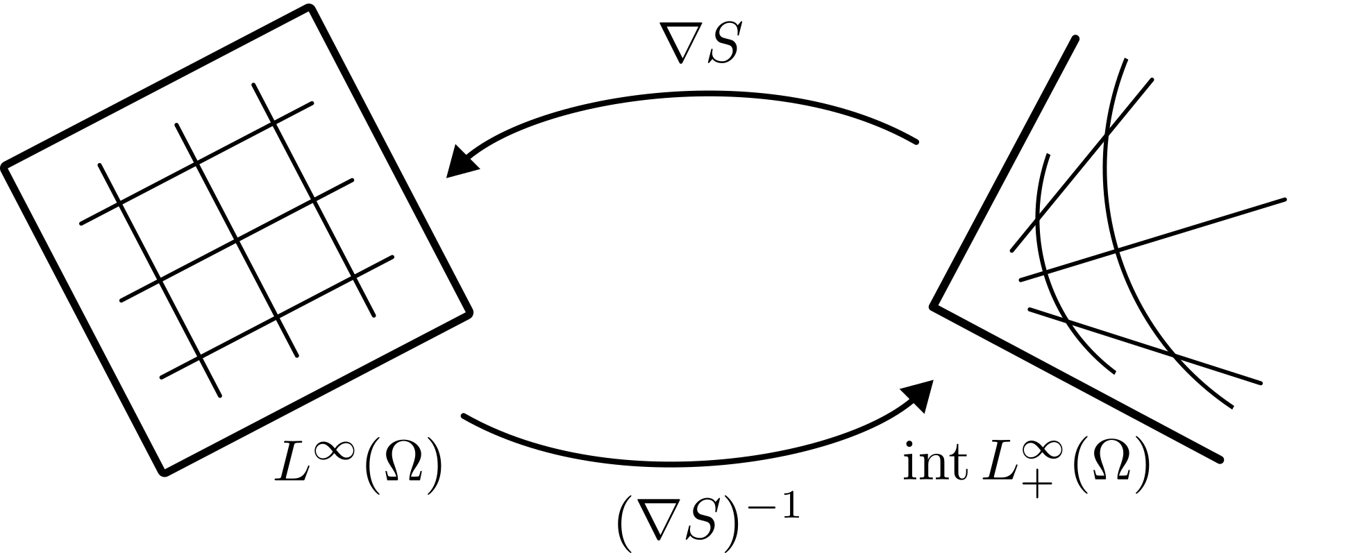
A deeper geometric meaning to this correspondence is revealed if we draw upon the well-known result in differential geometry that all finite-dimensional Lie groups are associated to their Lie algebra by an exponential map [133, Proposition 20.8]. In the case of the Lie group , it may be checked that the inverse of , defined , is precisely this map. Conveniently, the finite-dimensional result extends to the Banach–Lie group [77, 78], and we are left with a similar geometric interpretation (cf. fig. 2) of the isomorphism induced by the gradient of the entropy functional and its inverse,
| (46) |
Moreover, it can be shown that restricting the exponential map eq. 46 to the subalgebra induces an isomorphism with the subgroup . For further details, see Propositions 39 and 40.
Remark 9 (Exploiting the geometry of the feasible set).
From the optimization point-of-view, there is great value in the isomorphism residing in the fact that is a Banach space and Banach spaces are natural spaces in which to construct additive update formulas (they are complete, normed, and closed under addition). Many competitive algorithms for unconstrained optimization problems, such as gradient descent and Newton methods, are additive update formulas that leverage this linear structure in some way [166]. Likewise, when dealing with constrained optimization problems, most algorithms appeal to the linear structure of the ambient space containing the feasible set. In Section 4.4, we will show how the isomorphism allows us to ignore the ambient space the original problem is posed in and work instead with the intrinsic geometry of the constraint set. This, in turn, will allow us to treat constrained optimization problems in Sobolev spaces with methods originally designed only for the unconstrained setting.
4.3 Relative entropy
Entropy not only delivers an isomorphism between the Banach–Lie group and its Banach algebra . It also induces a valuable distance function called the relative entropy or (extended) Kullback–Leibler divergence.
We assume below that is a Banach space. For any smooth convex function , its Bregman divergence is defined by the formula
| (47) |
Encoded in this definition is the important observation that, because is convex, the graph will always lie on or above its supporting hyperplanes, , for every at which exists, see [38] for this and related insights. The Bregman divergence measures the vertical distance between these two sets.
Loosely speaking, a Bregman divergence is a generalization of the squared distance between two points in a Hilbert space. Indeed, it is a straightforward exercise to check, e.g., that if , with , the associated Bregman divergence is .
The relative entropy , for , is the Bregman divergence induced by the entropy functional . Given its importance to this work, we neglect to write the subscript- when working with this measure of distance. In turn, we may select any and to explicitly derive the relative entropy as follows,
| (48) |
An illustration of the Bregman divergence of the finite-dimensional entropy function is given in Figure 3 for the case . We initially use the right-hand side of eq. 48 in our study below without requiring its definition as a Bregman divergence. After a careful analysis shows that the relevant solutions are in , we then employ the usual properties of Bregman divergences where required in several convergence proofs. This frees us from the rigid structures of convex analysis, e.g., that often fix the domain in the beginning and require us to work only in this space and its given topology.
Along with other statistical distances, the relative entropy has a rich history of being used to encode geometric structure in analysis within statistics, probability theory, and information theory [11, 10, 165]. Although a Bregman divergence is not symmetric, i.e., in general, it will satisfy the following important properties when is strictly convex [38, 49]:
Proposition 10 (Properties of Bregman divergences).
Let be smooth and strictly convex. Then the following properties hold:
Non-negativity. for all and .
Positivity. if and only if .
Convexity. is strictly convex in its first argument. Moreover, if is strongly convex, then so is .
Linearity. Let be smooth and strictly convex and . Then
| (49) |
Three points identity. For all and , it holds that
| (50) |
4.4 Proximal point
Recall that in Section 2.2 we proposed the regularized Dirichlet free energy functional
| (51) |
and asserted that its minimizer will converge to the solution of the obstacle problem in the limit ; cf. eq. 26. Although this approach to solving the non-negative obstacle problem is viable, there is a much more numerically stable alternative. Indeed, it turns out that we can just as readily generate a sequence of positive functions by recursively regularizing the Dirichlet energy with the Bregman divergence . The idea is relatively old in finite dimensions [47, 197, 49, 198], and well-explored in reflexive Banach spaces [60, 59]. However, given that the algorithm is not well-known in the finite element community, we present a classical description that begins with a Hilbert space framework.
We now introduce the so-called proximal point algorithm [178, 170, 198], due to Marinet [151]. In turn, let be a Hilbert space and be a positive step size parameter. The proximal operator, introduced in [160] by Moreau, is defined for every proper lower semi-continuous function as follows,
| (52) |
The utility of this operator lies largely in the fact that the -regularization term in eq. 52 transforms (which may not be differentiable) into a finite-valued function,
| (53) |
with an -Lipschitz continuous gradient [178]. Moreover, when is convex, minimizing either or is equivalent in the sense that
| (54) |
In fact, the set of minimizers, , coincides with the set of fixed points that satisfy ; see, e.g., [24, Prop. 12.28].
Choosing to iterate this fixed point equation with variable step sizes delivers the proximal point algorithm [151, 177], written explicitly as
| (55) |
It is well-known (see, e.g., [87]), that converges to at a rate inversely proportional to the sum of the step sizes. More explicitly, it holds that
| (56) |
Thus, the function values of proximal iterates eq. 55 can converge “arbitrarily” fast (by increasing ), and the asymptotic complexity of the iteration eq. 55 is determined by the complexity of the method used to solve each subproblem eq. 52. Convergence of the function values carries over to convergence of the iterates provided an estimate of the type
holds, where is monotone and invertible on , e.g., if is strongly convex.
The potentially arbitrary order of convergence in eq. 56 makes the proximal point algorithm an attractive candidate to solve many optimization problems. The drawback, however, is that each iteration of the algorithm requires the solution of a nonsmooth optimization problem that may be just as difficult to solve as the original problem; cf. remark 15. At the same time, the proximal operator eq. 52 and fixed point iterations eq. 55 are fundamental to a broad selection of modern optimization algorithms; see e.g., [24, 25, 198, 126] and the many references therein. They also play a deep role in augmented Lagrangian methods, as recognized at least as early as [176], which have seen a resurgence in interest due, in part, to their applicability for infinite dimensional problems [111, 18].
It turns out many of the most important properties of the proximal point algorithm also hold if in eq. 52 is replaced by a Bregman divergence [198]. Indeed, if we assume that is a strictly convex functional on a Banach space , we may define the Bregman proximal operator
| (57) |
and the corresponding Bregman proximal point algorithm
| (58) |
Figure 3 illustrates the execution of this algorithm for the one-dimensional energy function and the relative entropy . Note that under the definitions above, one can show that eq. 56 generalizes as follows [49],
| (59) |
See also Theorem 17.
Our contribution is to show that the proximal operator eq. 57, with an appropriately defined Bregman divergence, transforms the solution of an infinite-dimensional constrained optimization problem into a sequence of semi-linear PDEs whose solutions converge to the solution of the underlying VI. In the case of the positive obstacle problem (i.e., and ), this conclusion hinges on the following result. When combined with eq. 58, Theorem 11 leads us directly to Algorithm 1, which forms the basis for the proximal Galerkin finite element method. We note that the proof is technical and saved until Section A.3.
Theorem 11 (Solution characterization).
Assume is an open, bounded Lipschitz domain, . Let , where satisfies . Moreover, given , set
and for set Then, for any step size , the (relative) Dirichlet free energy minimization problem,
| (60) |
has a unique solution that is (uniquely) characterized by the weak form of the entropic Poisson equation; namely,
| (61) |
Remark 12 (Adaptive entropy regularization).
Similar to the free energy formulation eq. 23, where the Lagrange multiplier is approximated by , we see that the subproblems eq. 61 give rise to an approximation of the form . Recalling that we see that there is fundamental difference in the two approximations given by the inclusion of the function . Chosen correctly, as with in eq. 58, this function can act as an informative prior on the sequence of subproblems. More specifically, allows us to view the Bregman divergence as a biased barrier function that is updated adaptively at each iteration so that without sending the step size .
From now on, we mainly focus on inhomogeneous obstacle problems; i.e., . Therefore, we close this subsection with an important corollary for this case. Before we state the result, we note that
whenever and . Therefore, is a Bregman divergence on . For technical reasons, we require the obstacles to be in a particular subset of defined by
| (62) |
Moreover, like theorem 11, the proof of Corollary 13 is delayed until Section A.3.
Corollary 13 (Solution characterization for inhomogeneous obstacles).
In addition to the assumptions of Theorem 11, let such that on and define
Then for any step size and the optimization problem
| (63) |
has a unique solution that satisfies the weak form of the (generalized) entropic Poisson equation; namely,
| (64) |
Remark 14 (Delicate analysis).
Semilinear mixed variational inequalities of obstacle type have been thoroughly studied, as detailed in the famous monograph by J.-F. Rodrigues, [179, Chap. 4.6]. This includes regularity theory and a maximum principle that relates the solution of the VI to the obstacle, forcing term, and boundary values. The techniques go back to the seminal work by Stampacchia [189], Murty and Stampacchia [162] and can also be found in [117]. However, the VI associated with our problem is only valid if we can differentiate the “extra” nonlinearity in the entropy term. This in turn requires the solution of each subproblem to be essentially bounded and strictly above the obstacle, so we need to resort to a more delicate analysis solely based on the properties of the optimization problem.
Remark 15 (Challenges of the Hilbert space setting).
Let denote the indicator function if and otherwise. It is interesting to compare the operator
| (65) |
to . Indeed, unlike eq. 61, the subproblems that eq. 65 induces each require the solution of their own VI,
| (66) |
that is at least as difficult to solve as the original VI defining ; cf. eq. 3. Similar issues tend to appear whenever squared norm regularization terms are used to design proximal point algorithms for infinite-dimensional bound constraints.
Alternatively, one can use a penalty method to solve the original problem by considering instead a -quadratic penalty term of the type
This functional is in fact the prox-operator (in the topology) of the indicator function for the larger feasible set . See [97, 96] for details including second-order algorithms and an analytical path-following scheme for . Note that the subproblems using a quadratic penalty would be semismooth semilinear elliptic PDEs. However, since the nonlinearity does not arise from a strictly monotone continuous function, we cannot derive a similar latent variable formulation.
Remark 16 (Comparison to the augmented Lagrangian method).
It is possible to view classical augmented Lagrangian methods as penalty methods that adaptively change the penalty function and associated penalty parameter via the behavior of the dual variable, i.e., Lagrange multiplier. Aside from identifying an efficient subproblem solver, the challenge is usually to find an appropriate combination of update strategies that allow for inexact subproblem solves and conservative parameter update rules that still exhibit rapid convergence behavior in practice. The method described in this work follows a similar strategy. Indeed, the role of the penalty function is played by a Bregman distance, which is adaptively updated via the primal variable, and the penalty parameter is given by . Bregman distances allow us to better exploit the geometry of the feasible set and the convergence theory of the proximal point method provides a clear connection to convergence rates that even allows for to remain constant.
4.5 Latent variable proximal point
An appealing feature of the entropic Poisson equation eq. 64 is that its solution permits two additional representations; cf. Figure 1. In both cases, we take advantage of the entropy gradient being an isomorphism (cf. Section 4.2). First, we may introduce the latent variable representation,
| (67) |
by simply applying the entropy gradient transformation to the primal solution . Second, as already noted in Remark 12, we may construct a dual variable representation which, for the inhomogeneous obstacle problem, is written as follows:
| (68) |
The utility of these representations is witnessed if we consider how to solve either of the primal subproblems eq. 61 or eq. 64. Indeed, due to the logarithmic terms, these semi-linear PDEs are only defined if , which appears to rule out most efficient root-finding algorithms, such as Newton’s method, and discretization choices, such as the Galerkin method. Fortunately, the alternative solution representations above provide saddle-point relaxations of the entropic Poisson equation that do not suffer from these two drawbacks.
We are now ready to state the final main theoretical result, which also establishes explicit bounds on the optimization error for the latent variable proximal point (LVPP) algorithm, defined via eq. 69 below. The proof is given in Section A.4.
Theorem 17 (Convergence of LVPP).
Assume , , is a sequence of positive step size parameters. Furthermore, assume is an open, bounded Lipschitz domain, , , and let such that . Fix and consider the sequence of functions , solving the following coupled system of variational equations:
| (69) |
Then the Dirichlet energy of the primal iterates is monotonically non-increasing, i.e.,
| (70) |
Moreover, if as , then the subproblem solutions converge in to
| (71) |
Furthermore, the functions converge strongly in to the Lagrange multiplier . In fact, the optimization error in both and are equal and converge at the following arbitrary rate determined by the sequence of step-sizes ,
| (72) |
Remark 18 (Arbitrary orders of convergence).
Theorem 17 shows that the iteration complexity of LVPP depends on the choice of the step sizes . The consequences of different step size choices is summarized in Corollary 44. For example, we find that constant step sizes lead to sublinear convergence and geometrically increasing step sizes lead to first-order convergence. Even faster growing step size sequences will achieve superlinear convergence. See also Remark 22.
Remark 19 (Convergence in the -norm).
At first glance, control over the full norm of appears problematic because eq. 72 does not include the full norm on . However, in light of the Poincaré inequality and , we also obtain
where is an embedding constant independent of .
Remark 20 (Convergence of the latent variable).
If we adopt the conventions and , we may define as an extended real-valued function on ; cf. Section 2.1. Likewise, we may understand convergence of the latent variable under the metric implied by this transformation. Indeed, consider the metric , first introduced in eq. 17. Clearly,
| (73) |
which converges to zero as by eq. 72.
Remark 21 (Dual variable mixed formulation).
The formulation eq. 69 is derived by setting , , and substituting the equation into eq. 64. If, instead, we considered the dual variable substitution , we would arrive at the following alternative formulation:
| (74) |
Although this is equivalent to eq. 69 at the continuous level, it will induce a different Galerkin method; cf. Section 4.6. We leave the study of such dual variable proximal Galerkin methods for future research.
Remark 22 (Strict complementarity).
Although Theorem 17 allows us to establish arbitrary orders of convergence (see Corollary 44), it still represents the worst-case iteration complexity. In particular, our numerical experiments in Section 4.8.2, suggest that an improved result may be possible if the solution exhibits strict complementarity.
4.6 Proximal Galerkin
Motivated by Theorem 17, it is natural to use finite-dimensional subspaces and in order to form a Galerkin discretization of eq. 69. Thus, we arrive at Algorithm 3, which may be seen as a natural extension of Algorithm 2 to the inhomogeneous obstacle problem.
| (75) |
Just like Algorithm 2, we find that Algorithm 3 delivers two distinct approximations of the exact solution; and . The second of these approximations is unusual because it is guaranteed to satisfy the inequality . Moreover, like the continuous-level algorithm in Theorem 17, it also produces an approximate Lagrange multiplier,
| (76) |
where denotes the final iterate where the abstract convergence test in Algorithm 3 is satisfied.
Finite element methods typically lead to piece-wise polynomial approximations of the exact solution. Given that relies on a non-standard type of exponential function approximation, it is natural ask whether can produce an accurate approximation of the continuous-level solution . The following result provides a partial positive answer to this question. The proof is given in Section B.3.
Proposition 23 (Approximability).
Let and define . Moreover, let and . The following identity holds:
| (77) |
The next ordinary concern would be the stability of the discretization eq. 75. In the next subsection, we propose stable pairs of finite elements that can be used to construct and .
4.7 Stable pairs of finite elements I: Discontinuous latent variable
Subspace pairings determine the stability of finite element methods for saddle-point problems [34]. Thus, it should come as no surprise that choosing compatible subspaces and is central to the proximal Galerkin method. In this section, we choose to focus on stable pairs of finite elements with discontinuous latent variables , as these appear to provide the most efficient approximations per degree of freedom. The elements we propose are defined in eq. 79, below.
Remark 24 (Continuous latent variables).
In Section 5.3, we propose a simple type of equal-order Lagrange element discretization employing a continuous latent variable . Although this compatible discretization has numerous interesting properties, including providing a feasible, -conforming discrete solution , we have been unable prove that these elements are stable under as general a set of assumptions as the elements proposed here. The elements proposed in Section 5.3 are also less efficient with respect to degrees of freedom.
Remark 25 (Other stable pairs).
Alternative finite element discretizations employing macroelement partitions (e.g., [190]), various non-conforming approximation techniques (e.g., [56, 51]), or even spline-based approximation spaces (cf. [104]) all provide possible alternatives for the design of proximal Galerkin methods. Due to space in this manuscript and the limitations of our present software, we leave these and other possible constructions to future studies.
4.7.1 Finite element notation
Here and throughout, always denotes a shape-regular [69, Chapter 11.1] partition of the domain , , into finitely many open connected triangular/tetrahedral or quadrilateral/hexahedral mesh cells with Lipschitz boundaries such that is the union of the closure of all mesh cells in . Following convention, denotes the mesh size , where . Let denote the space of polynomials of total degree up to and including on a triangle/tetrahedron . Likewise, let denote the space of tensor-product polynomials of partial degree up to and including on a quadrilateral/hexahedron [69, Chapter 6.4]. For any space of polynomials over an element , we abuse notation to denote the corresponding space of “broken” polynomials .
We will require spaces of degree- polynomials whose traces on the cell boundary have lower polynomial degree . To this end, define the sets of so-called bubble functions in and to be and , respectively. Accordingly, define and . Finally, let
| (78) |
4.7.2 Element definitions and properties
We are now ready to define the finite element spaces, which we chose based on a priori analysis of a simple linearization of subproblem eq. 75. For further details of the analysis, see Appendix B.
For any integer , we define the following two pairs of spaces:
Triangular/Tetrahedral elements. We refer to the following as the pairing:
| (79a) |
Quadrilateral/Hexahedral elements. We refer to the following as the pairing:
| (79b) |
Figure 5 provides a visual representation of the lowest-order versions of these elements.
Remark 26 (Positive cell average).
Assume . Although the piecewise polynomials that arise from solving the subproblems eq. 75 can not be guaranteed to preserve pointwise positivity, they are guaranteed to have positive cell averages. Indeed, notice that the subspaces in eq. 79 always include piecewise constant functions. Therefore, we may consider the second equation in eq. 75 with in and otherwise. Testing with this particular function implies that
| (80) |
If , then a similar argument implies that each cell average of lies above the corresponding cell average of .
Remark 27 (Alternative subspaces).
Although variable-order spaces like in eq. 79 are supported in some software [183, 76], they may not available in the preferred software of many users. For this reason, we also propose the following less efficient alternative pairings:
Alternative triangular/tetrahedral elements. We refer to the following as the subspaces:
| (81a) |
Alternative quadrilateral/hexahedral elements. We refer to the following as the subspaces:
| (81b) |
Since eq. 79 are stable (cf. Lemma 48), it is a straightforward consequence of the inclusions and that eq. 81 are also stable. For further details, see Remark 50.
4.8 Numerical experiments
We performed five sets of numerical experiments in order to validate the proximal Galerkin method. The first experiment involves a smooth biactive manufactured solution that allows us to verify the (mesh-independent) iteration complexity predicted by Theorem 17, in addition to high-order convergence rates with respect to the polynomial order of the finite element subspaces. In the second experiment, we check the discrete Karush–Kuhn–Tucker (KKT) conditions on a manufactured solution exhibiting strict complementarity. In this case, we observe better iteration complexity than predicted by Theorem 17. We conjecture that this improved convergence order holds in general whenever a strict complementarity condition is satisfied; cf. Remark 22. The third experiment involves a non-smooth biactive solution and is included to further stress test the proximal Galerkin method. In the fourth experiment, we consider a benchmark obstacle problem from the literature and demonstrate our ability solve this problem with the highest order finite elements currently supported in our MFEM implementation (); cf. Remark 28. Finally, our fifth experiment demonstrates good performance with a discontinuous obstacle on an adaptively-refined mesh. Thus, the regularity restriction required in the theory above is not essential in practice.
Each of our experiments were conducted on standard sequences of uniformly refined nested meshes conforming to unit ball domains in . The experiments with the triangular elements (FEniCSx) used an -unit ball (i.e., square) domain,
| (82a) | |||
| with initial mesh size denoted . Meanwhile, the experiments with the quadrilateral elements (MFEM) used an -unit ball (i.e., circular) domain, | |||
| (82b) | |||
with initial mesh size denoted , which was uniformly refined using a standard transfinite interpolation rule to handle the curvilinear element mappings [84]. The initial meshes in these sequences are depicted in Figure 6.
Remark 28 (Software implementations and reproducibility).
We conducted numerical experiments across two separate code bases, FEniCSx [186] and MFEM [14], and have released our implementations to the public [112, 114]. The FEniCSx implementation [114] is Python-based and uses the triangular elements proposed in Section 4.7. The MFEM implementation is written in C++. Because MFEM does not currently support bubble function enrichment, the MFEM implementation [112] uses quadrilateral elements (see Remark 27) instead of the elements also proposed in Section 4.7.
We have taken care to ensure that the numerical experiments in this section are easily reproducible. Indeed, all results from Experiments 1, 2, 3, and 5 can be reproduced by running the FEniCSx script obstacle.py or compiling and running the MFEM codes obstacle.cpp or obstacle_discontinuous.cpp, all of which are available at [114]. Experiment 4 now exists as an official part of the MFEM codebase called MFEM Example 36 [112].
4.8.1 Experiment 1: Smooth biactive solution
In this experiment, we set and , where is the smooth manufactured solution
| (83) |
See Figures 7 and 8 for depictions of the exact solution on and , respectively.
This problem is specifically chosen to exhibit biactivity; i.e., both the inequality constraint and the associated Lagrange multiplier are simultaneously equal to zero on a set of positive measure; i.e., on the set . Such problems are notoriously difficult to solve for certain classes of algorithms, such as active set methods. Biactivity, also know as weak activity or lack of strict complementarity, is a notion from nonlinear optimization that indicates a kind of degenerate nonsmoothness of the primal-dual system of equations used to calculate the solution. It is often associated with a lack of stability with respect to perturbations of the data, as well. We refer the interested reader to any standard text of numerical optimization; see, e.g., [166, Definition 12.5].
Our first aim is to use this challenging example to illustrate mesh-independence of the proximal Galerkin method. To this end, we use Table 1 to record the values of the increments taken from a sequence of refined meshes with polynomial orders from our FEniCSx implementation [114]. The specific step size rule used to generate this data is chosen based on Corollary 44 to deliver superlinear convergence (in iterations), and is given as follows:
| (84a) | |||
| where . Note that, for each iteration , the increments in Table 1 converge to fixed values as the mesh is refined or the polynomial order is raised. Moreover, the total number of linear equation solves remains bounded. Both of these characteristics are emblematic of a mesh-independent numerical method. | |||
| Progress of the iterates for various and | ||||||
| Polynomial order | Polynomial order | |||||
| 1 | ||||||
| 2 | ||||||
| 3 | ||||||
| 4 | ||||||
| 5 | ||||||
| 6 | ||||||
| 7 | ||||||
| 8 | ||||||
| 9 | ||||||
| 10 | ||||||
| 11 | ||||||
| 12 | ||||||
| Tot. linear solves | ||||||
Our next aim is to verify the convergence orders predicted by Theorem 17 and Corollary 44. In doing so, we consider the double-exponential step size rule eq. 84a alongside the geometric rule
| (84b) |
with , and the fixed step size rule , for all The results in Figure 7 agree precisely with the predictions made later on in Corollary 44. In particular, notice that the fixed step rule leads to sublinear convergence, the geometric rule eq. 84b induces linear convergence, and the double-exponential step size rule eq. 84a delivers superlinear convergence.
The final aim of this experiment is to demonstrate that high-order convergence rates (with respect to the mesh size ) can be achieved using polynomial orders . To this end, we use our high-order MFEM implementation to solve for the biactive solution eq. 83 on the circular domain . In Figure 8, we plot the approximation errors of the discrete solutions , , and . From these results, we witness that high-order convergence rates can, indeed, be achieved with the proximal Galerkin method.
4.8.2 Experiment 2: Strict complementarity
In this experiment, we set and define
| (85) |
See Figure 9 for a fine mesh () solution as well as the associated Lagrange multiplier .
When viewed from the perspective of continuum mechanics, the multiplier is a resolvent force. It is therefore rare that we would see biactivity of the type in the previous experiments on such large domains as it would correspond to contact without any opposing force resulting from the obstacle.
The first aim of this experiment is to revisit the convergence orders predicted by Theorem 17 and Corollary 44 and demonstrate that they are overly pessimistic for this more typical type of problem. Indeed, as demonstrated in Figure 9, we see that linear convergence is achieved using only a fixed step size. In turn, superlinear convergence can be achieved using any unbounded step size rule. For illustration, we have added results using the geometric rule eq. 84b with various growth parameters .
The second aim of this experiment is to check convergence of the discrete solution via the KKT conditions. This is useful to assess a posteriori the optimality of the discrete solution when the true solution is unknown. To this end, we consider the complementarity condition , the primal feasibility condition , and the dual feasibility condition . We note that the discrete solution always satisfies the primal feasibility condition by construction; i.e., . Therefore, in order to glean more interesting information about the proximal Galerkin solution, we focus on discrete versions of the KKT conditions formulated in terms of . The discrete KKT conditions that we checked are recorded in Table 2. From the results in this table, we see that discrete primal feasibility, , is achieved only in the limit . However, discrete complementarity, , and discrete dual feasibility, , appear to hold for all mesh sizes.
| Complementarity | Primal feasibility | Dual feasibility | |
|---|---|---|---|
| () | () | ||
4.8.3 Experiment 3: Biactive solution, nonsmooth multiplier
In this experiment, we set and , where is the smooth manufactured solution
| (86a) | |||
| implied by the forcing function | |||
| (86b) | |||
| Clearly, this is another solution exhibiting biactivity. In this case, however, the multiplier, | |||
| (86c) | |||
is discontinuous. See Figure 10 for a depiction of the exact solution as well as the associated Lagrange multiplier on the domain .
We use this experiment to inspect the approximation error of the discretization. See Figure 10 for our results. As expected, unlike for the biactive solution studied in Section 4.8.1, the -error of the Lagrange multiplier does not decay to zero linearly. We observed no other adverse effects from this non-smooth manufactured solution.
4.8.4 Experiment 4: Spherical obstacle
Our next experiment is motivated by an exact solution in [88]. Here, we set both and and define the obstacle to be the upper surface of a sphere of radius , namely
| (87) |
if , and assume that is sufficiently negative when so that no contact happens on that subdomain. Exploiting radial symmetry, the exact solution on the circular domain is found to be
| (88) |
where , , and is the -th branch of the Lambert W‐function.
Figure 11 presents the very high polynomial degree () proximal Galerkin solutions and to this problem on the coarsest mesh, , which has only five elements. We note that the solution to this problem is in , , which is the highest regularity guaranteed by a smooth obstacle and load [39]. Thus, we do not expect to achieve high-order accuracy with such a high degree discretization unless the mesh is adaptively refined [20]. Developing an a posteriori error estimator for proximal Galerkin in order to enact such adaptive mesh refinement strategies will be the subject of future work.
Table 3 compares the subproblem error, , on a sequence of uniformly-refined meshes. In order to include the more -refinements, we consider only the lowest-degree discretization (). However, we find similar results with higher ; cf. Table 1. To demonstrate that proximal Galerkin is practical without large step sizes, we fix for all iterations. In this case, we note that the method is now expected to converge with linear complexity due to the strict complementarity of the solution; cf. Section 4.8.2. From Table 3, we see that if the number of outer iterations is fixed, then the error converges to a single value as the mesh is refined. This is an important hallmark of mesh-independence.

Diagram of problem


Very high order () proximal Galerkin solutions (top) and (bottom)
| Primal errors for | ||||||
| Linear solves | ||||||
| 1 | 3 | |||||
| 2 | 1 | |||||
| 3 | 1 | |||||
| ⋮ | ⋮ | ⋮ | ⋮ | ⋮ | ⋮ | ⋮ |
| Total iterations | ||||||
| Total linear solves | ||||||
| Final error | ||||||
4.8.5 Experiment 5: Discontinuous obstacle
Our final experiment serves to test an important limitation of the mathematical theory presented in this section. In particular, we explore the performance of proximal Galerkin when the regularity condition (cf. eq. 62) is not satisfied. For simplicity, we set .
In this experiment, we consider the discontinuous obstacle,
| (89) |
on the circular domain , with no body force (), and homogeneous Dirichlet boundary conditions on . In this case, one can show that the exact solution is
| (90) |
To obtain an accurate discrete solution, we pre-process the mesh with adaptive refinements until the data oscillation error [161] in the obstacle,
is below . The corresponding mesh , obstacle , and solution are depicted in Figure 12. Starting with the same initial guess as in Experiment 4, we witnessed convergence to the depicted solution in only outer iterations of Algorithm 3 with total linear solves (inner Newton iterations). The corresponding -error is .


5 Extensions I: More general bound constraints and variational inequalities with an application to enforcing discrete maximum principles
The purpose of this section is to move beyond the framework developed in Section 4 for energy principles with pointwise lower bound constraints. To this end, we aim to answer the following two necessary questions:
- 1.
Can proximal Galerkin be used to simultaneously enforce pointwise upper and lower bound constraints?
- 2.
Can proximal Galerkin be applied to variational inequalities that do not arise from an energy minimization principle?
The answer to both of these questions is yes.
We use our answers to these questions to construct a discrete maximum principle-preserving proximal Galerkin method for the advection-diffusion equation,
| (91) |
where and are fixed, , and . Along the way, we introduce the binary entropy (Section 5.1), a proximal algorithm for VIs with non-symmetric coercive bilinear forms (Section 5.2), and an alternative type of proximal Galerkin discretization employing a continuous latent variable (Section 5.3). The section features an implementable algorithm and closes with a brief survey of numerical experiments.
5.1 Binary entropy
In the previous section, enforcing a pointwise lower bound on the minimizer of the Dirichlet energy led us to consider a sequence of entropy-regularized energy minimization problems. We now consider the situation of enforcing pointwise upper and lower bounds simultaneously. For simplicity, we illustrate the approach on the so-called double-obstacle problem written in eq. 92 below.
Let with and , and consider minimizing the Dirichlet energy under the pointwise bound constraints . More specifically,
| (92) |
where and . A natural way to apply entropy regularization to eq. 92 is revealed if we rewrite the problem with two new variables and . Doing so, we arrive at the equivalent equality-constrained optimization problem
| (93) |
where and . It can be readily verified that and .
Following our treatment of entropy regularization for pointwise non-negativity constraints in Section 4, it stands to consider the sequence defined
| (94a) | ||||
| (94b) | ||||
We may now resubstitute and into eq. 94a, which leads to
| (95) |
where
| (96) |
is the Bregman divergence of the (generalized) binary entropy
| (97) |
A straight-forward computation shows that
| (98) |
The cases and are somewhat special for the binary entropy functional eq. 97. In the first of these, eq. 97 is usually referred to as the (negative) Fermi–Dirac or electronic entropy [198]. As these particular upper and lower bounds will appear prominently later on, we choose to adopt special notation for the corresponding entropy gradient and its inverse; namely,
| (99) |
The second case, , provides a gradient that is an explicit diffeomorphism between the -unit ball, denoted , and the entire Banach algebra . More explicitly, we write
| (100) |
with the diffeomorphism illustrated visually in Figure 13. For posterity, we use the latter case of the binary entropy functional to define a canonical binary-entropic Poisson equation,
| (101) |
which follows from writing the strong form of the first-order optimality condition for eq. 95 with , , , , and removing the factor of in eq. 100.
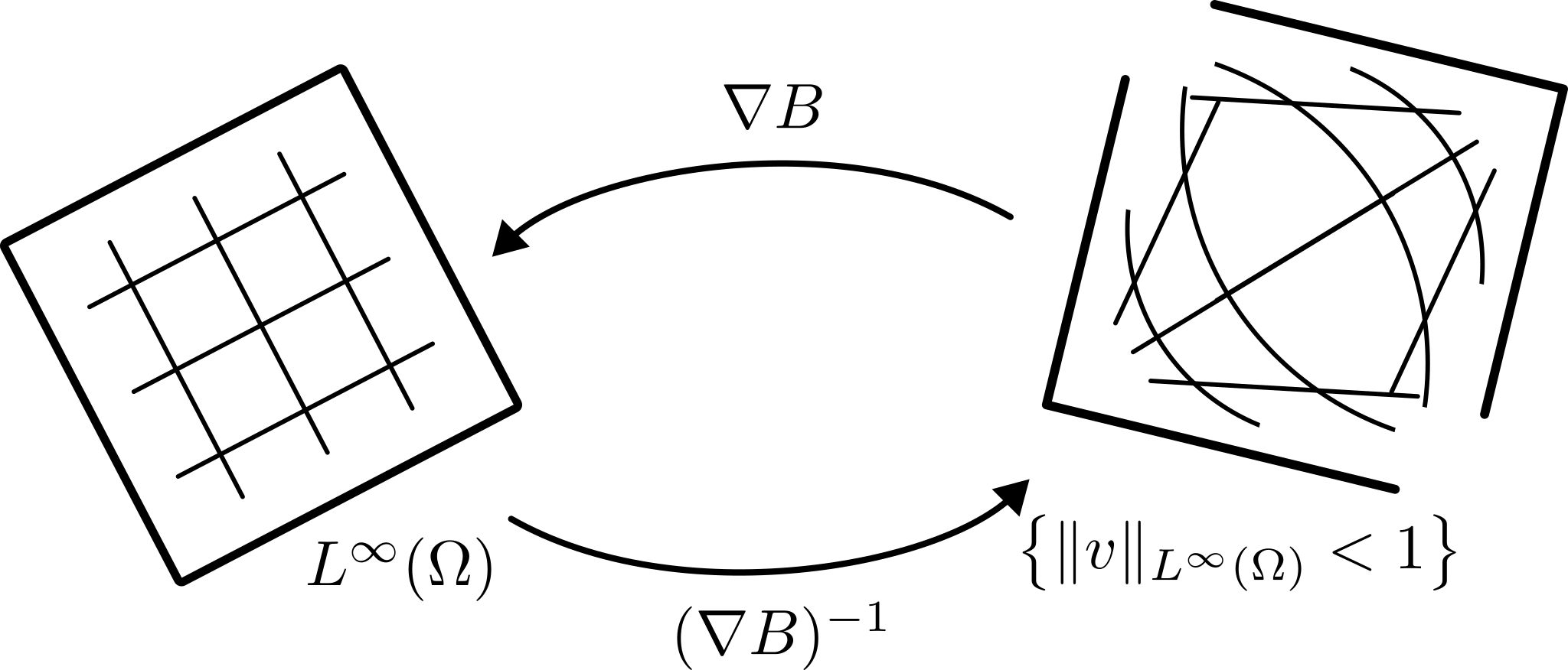
5.2 Variational inequalities with non-symmetric bilinear forms
In order to develop a proximal Galerkin method for the advection-diffusion equation eq. 91, we first propose a continuous-level proximal algorithm for non-symmetric bilinear forms. The approach is based on the proof technique for the classical theorem of Lions and Stampacchia on the existence of solutions to elliptic variational inequalities with non-symmetric bilinear forms, which can be understood as employing a “linearized” version of algorithm eq. 55.
Assume that is a real separable Hilbert space and is bilinear, continuous, and coercive. In particular, assume that there exist constants such that
| (102) |
for all . For any nonempty closed convex set and function , the Lions–Stampacchia theorem [141] states that the following variational inequality is well-posed:
| (103) |
The proof works by arguing that for , the mapping , defined as the unique solution of the problem
| (104a) | |||
| is a contraction. Note that we may equivalently write | |||
| (104b) | |||
| which illustrates the following relationship to the proximal operator introduced in Section 4.4, . Clearly, if we find the fixed point , then eq. 104a reduces to eq. 103 and we deduce that . | |||
This method of successive approximations,
| (104c) |
is well-known and has been analyzed in, e.g., [200]. However, it is not exactly amenable to computation because it requires a separate subproblem solver for each of the VIs eq. 104a. Since is typically not known in practice, it is common to select diminishing step sizes to analyze the convergence behavior. In addition, different strategies may be employed using extrapolation steps, see related methods in, e.g., [126]. We postpone a deeper analysis for future work. Given a set with appropriate structure, we can circumvent this issue using the proximal Galerkin methodology.
We begin by regularizing the continuous-level subproblems eq. 104a. A first approach would be to use the Bregman proximal point algorithm eq. 58 to solve the subproblems to an iteration-dependent tolerance . This would result in a sequence of inexact successive approximations that could converge to if the sequence of tolerances decays to zero as . The potential drawback of this approach is that it creates an additional nested sequence of iterations. In turn, generating each iterate may require numerous individual proximal point iterations eq. 58 for every inexact fixed point iteration .
Instead of using the Bregman proximal point algorithm as a subproblem solver, we propose to modify the original fixed point map eq. 104b by adding an additional Bregman divergence term. More specifically, we propose considering the alternative fixed-point iteration
| (105a) | |||
| where is a strictly convex entropy functional associated to the feasible set and is an operator formally defined for all as follows: | |||
| (105b) | |||
Returning to the advection-diffusion problem eq. 91, we now assume that a.e., , and , where is such that and . Instead of iterating the fixed point operator for some , we propose to generate a sequence of iterates from eq. 105 with set to be the binary entropy considered in eq. 99. More explicitly, we choose an appropriate and a sequence of positive real numbers, and then solve the sequence of resulting subproblems
| (106) |
Once discretized with a slack variable , we arrive at the algorithm written below.
| (107) |
5.3 Stable elements II: Continuous latent variable
Constructing a stable finite element discretization for Algorithm 4 has the same challenges we witnessed in solving the obstacle problem with Algorithm 3. Namely, we must construct a stable pair of finite element subspaces and . To this end, Section 4.7 introduced a class of possible pairings based on the requirement that the latent variable be discontinuous. We could use the same finite elements here because the saddle-point problem eq. 107 has the same structure after linearization as eq. 75. Instead, however, we use this subsection to introduce the following alternative class of equal-order finite element pairings where is continuous.
For any integer , we define the following two pairs of spaces:
Triangular elements. We refer to the following as the pairing:
| (108a) |
Quadrilateral elements. We refer to the following as the pairing:
| (108b) |
Figure 14 provides a visual representation of the lowest-order versions of these elements.
The equal-order finite element subspaces in eq. 108 are appealing because they can be formed from standard -finite elements that are found in nearly all production codes. However, due to limitations of the stability proof outlined in Remark 30, we only advocate for using these elements when the mesh sequence is quasi-uniform [69, Definition 22.20].
Definition 29 (Quasi-uniformity).
A shape-regular sequence of meshes is called quasi-uniform when there exists a mesh-independent constant such that for all and all in the index set.
A careful inspection of Appendix B shows that we do not need to place such a restriction on the mesh when using the non-standard elements proposed in Section 4.7.
In addition to the quasi-uniformity assumption above, the reader may notice that the number of degrees of freedom per element pair in eq. 108 is larger than that of the analogous order- pairs proposed in eq. 79. We pause to point out that neither of these factors preclude using eq. 108 in practical applications. Indeed, many practical applications are solved on quasi-uniform meshes. Moreover, it turns out that the additional computational cost can be mitigated via a mass lumping technique described in Remark 31 below.
As also explained in this remark, a particularly interesting consequence of mass lumping is that it induces a nodally bound-preserving primal solution . Moreover, because nodal boundedness extends to pointwise boundedness when , the primal solution will be pointwise bound-preserving for any lowest-order or proximal Galerkin discretization with box constraints. In contrast, the lowest-order elements in eq. 79 only induce a primal discretization with a bound-preserving cell average; cf. Remark 26.
Remark 30 (Stability).
As described in Appendix B, uniform stability of the proximal Galerkin discretization rests on satisfying the Ladyzhenskaya–Babuška–Brezzi (LBB) condition
| (109) |
with independent of the mesh size . Verifying this condition is often nontrivial. However, it reduces to a one-line argument given in eq. 111 below if the global -orthogonal projection , defined
| (110a) | |||
| is stable in the (equivalent) -norm; i.e., if there exists a constant , independent of , such that | |||
| (110b) | |||
| for all . | |||
Remark 31 (Nodal bound preservation).
We choose to focus this remark on the saddle-point problem in Algorithm 4. Yet, similar conclusions could be drawn about Algorithm 3 and, potentially, other future proximal Galerkin algorithms for second-order elliptic VIs.
Consider the equal-order finite element subspaces in eq. 108 and let be a basis for . It follows that there exist coefficients and , , such that and . Substituting these expressions into the second variational equation in eq. 107, setting , and replacing the Lebesgue integral with a global quadrature rule , where and for , we find that
| (112) |
for each index .
We now employ the nodal-quadrature mass lumping technique [74] that is commonly used in, e.g., spectral element methods [63]. Although this quadrature technique is applied to the linearized form of eq. 112, the effect on the solution is equivalent to modifying the nonlinear equation directly, as described below. Assume and that are formed from a nodal basis with nodes corresponding to the quadrature points (e.g., a Lagrange basis with Gauss–Lobatto nodes [174]). Thus, for all . Moreover, we find that eq. 112 reduces to
| (113) |
Finally, notice that and since we have assumed the basis is nodal. Thus, the primal variable is nodally bound preserving; i.e., at all points , .
5.4 Numerical experiments
In this set of experiments, we follow [48, Section 4.1] and consider the exact solution of a model problem attributed to Eriksson and Johnson [66]. In particular, we set , , and in eq. 91 and, therefore, write
| (114) |
Exact solutions of this problem for arbitrary boundary data can be derived using the separation of variables technique. We choose to isolate the solutions satisfying where and where and . Doing so generates the following series expansion:
| (115) |
where and . Note that the constants can be determined from the prescribed values of on . Since we have not yet prescribed on this part of the boundary, we define there to be eq. 115 with and ; i.e, we treat the first mode in this series as a manufactured solution for eq. 114.
Figure 15 places the standard FEM solution of this problem for alongside the corresponding maximum principle-preserving proximal Galerkin solution . Here, the proximal Galerkin solution can be found by running only two iterations of Algorithm 4 with constant values for and , and using the standard first-order FEM solution to provide an initial guess for and . Note that the two discrete solutions are similar, except the proximal Galerkin solution preserves the maximum principle . We also experimented with using the mass lumping technique described in Section 5.3. The results of this experiment are given in Figure 16. Here, note that both the the primal solution and the latent variable solution are bound-preserving in this case. For further details, or to reproduce the our experiments, the interested reader is directed to our open-source FEniCSx and MFEM implementations found at [114].

Exact solution

 FEM solution
 Proximal Galerkin solution
Without lumping:


With lumping:


Note that neither of the numerical approximations depicted in Figures 15 and 16 were obtained with numerical stabilization techniques that are common for this class of singularly-perturbed problems and usually required to avoid spurious oscillations for smaller values of . Just as conventional stabilized finite element methods do not necessarily preserve maximum principles [71], we find that entropy regularization does not necessarily induce robustness with respect to the diffusion parameter . In turn, we observe spurious oscillations in the discrete solution for smaller values of . Our conclusion is, therefore, that future work is required to develop robust proximal Galerkin finite element methods for singularly-perturbed PDEs.
6 Extensions II: Non-convex objective functions and a structure-preserving algorithm for topology optimization
The variational problems considered in the sections above share several common features. The most decisive feature is convexity. This raises the question as to whether entropy regularization can be as effective in a non-convex infinite-dimensional setting. We investigate this possibility here by providing a new proximal gradient (entropic mirror descent) framework for possibly non-convex, bounded-constrained optimization in infinite dimensions. Our benchmark problem for this setting is a well-known problem in topology optimization. As before, the section closes with an explicit algorithm and a brief account of numerical experiments. In the interest of completeness, we recall several details from abstract mirror descent methods. Although these methods are widely used in finite-dimensional convex optimization, and much of our treatment is inspired by the more recent works [26, 198], it is important to note that Nemirovskij and Yudin did not restrict themselves to finite dimensions in their original works many decades ago [163, 164].
6.1 Mirror descent
Section 4.4 introduced a proximal framework that was applied to solve the obstacle problem. Section 5.2 introduced a linearized proximal framework to solve variational inequalities with non-symmetric bilinear forms. The purpose of the present subsection is to combine those two approaches into a general first-order framework for non-convex optimization problems,
| (116) |
where is a nonempty, closed convex subset of a Banach space and is continuously Fréchet differentiable. We closely follow [26, 198] below to provide intuition for the method. In several places, we are purposely vague. This is particularly the case for the assumption that a Bregman divergence induced by the derivative is available or that is non-empty with respect to the topology on .
We begin by introducing the Bregman gradient step operator,
| (117) |
where is strongly convex with derivative . When is a Hilbert space and , the use of the gradient step operator leads to the standard gradient descent rule. This follows from a straightforward computation of the first-order optimality criteria, which leads to
| (118) |
where is the gradient of characterized by the variational equation
| (119) |
More generally, assuming the minimizer exists and is invertible, eq. 117 returns the formula
| (120) |
Recalling the classical steepest descent method, see, e.g., [166], it is not surprisingly that iterating eq. 117 can generate a convergent algorithm to solve eq. 116 when and an appropriate step size rule for is available. Indeed, convergence of this algorithm is illustrated in fig. 17 for optimizing the scalar objective function with the Bregman divergence from the scalar entropy function . This naturally leads to the so-called mirror descent method [164, 26], which, given a sequence of positive step sizes , generates a sequence of iterates according to the following scheme:
Nemirovskij and Yudin point out that the motion of the iterates , which takes place in the primal space , is a “shadow” or “image”, of the main motion: , which by definition takes place in the dual space; whence the name “method of mirror descent” [164, p. 88]. This is easily witnessed by introducing a dual variable . Then under the assumptions that is invertible, the new step in the dual space takes a somewhat more familiar form:
This important distinction is often lost in finite dimensions and to some extent in the Hilbert space setting, where and are often identified with their Riesz representations in ; i.e., the gradients and , respectively.
6.2 Mirror descent with a linear equality constraint
For constrained problems, it is essential that properly captures the geometry of the feasible set, as was done in the previous sections on the obstacle problem and advection-diffusion equations. Many problems of interest have the following form:
| (121) |
where and are nonempty, closed convex subsets of and is differentiable. For example, suppose that is a nonempty, closed convex set and for some linear functional and constant ; i.e., . Furthermore, suppose that is a Bregman divergence associated with a distance generating function , which is a Legendre function whose critical domain is linked to the properties of . In this setting, we fix and define the operator
We assume here that over has all the properties needed to ensure is single-valued. Using standard optimality theory, e.g., [107], we can argue that satisfies the inclusion
| (122) |
where is the normal cone from convex analysis [107], defined by
Note that if , then eq. 122 reduces to
which indicates that is a first-order stationary point of eq. 121.
If we furthermore assume that contains a subset such that , for some , then contains an open neighborhood of . This constraint qualification [107] allows us to rewrite eq. 122 as
| (123) |
where provided . Continuing on, we may assume for the sake of argument that the use of forces and . This happens, for example, if remains away from the boundary of . For pointwise bound constraints in -spaces of the type considered below, we would also have when almost everywhere, even if the set has an empty interior. The remaining normal cone is trivial to compute and yields .
These observations justify the following first-order optimality system that characterizes the map : Find such that
| (124) |
In other words, given and , compute the increment and find by solving the equation
Repeating the process
generates a sequence of primal variables. Indeed, given a sequence of positive step sizes , we can generate according to Algorithm 5.
The pre-image of is tacitly assumed to be contained in . Therefore, the abstract scheme Algorithm 5 theoretically provides a sequence of feasible primal iterates
Checking for optimality is rather difficult in general, as the evaluation of the residual of first-order optimality conditions may require the computation of a projection operator in non-trivial settings; recall the discussion in Remark 15 above. On the other hand, we demonstrated above that fixed points of are stationary for the original problem. This motivates the simple stopping rule: , with sufficiently small, or some variant using absolute and relative tolerances. However, in order to remove the influence of , which will typically change with , we advocate for rescaling the fixed point residual and also consider the relative quantities
In the unconstrained Hilbert-space setting, we have . Therefore, if , then ; i.e., we get a limiting stationarity condition. For example, if is a null sequence in for , then clearly . We therefore also use as a heuristic stopping measure in our experiments below.
The abstract derivation above yields an iterative scheme in the dual space . Implementing finite-dimensional approximations of negative-order Sobolev spaces can be challenging. However, the bound-constrained variational problem we have considered happens to have a substantial degree of useful structure, and entropy regularization of the associated bound constraints provides us with representations of , and that lead to a latent space reformulation of Algorithm 5 that is readily treated with finite elements.
6.3 An entropic mirror descent algorithm for topology optimization
We consider the benchmark topology optimization problem of elastic compliance optimization of a cantilever beam; see, e.g., [16]. In particular, we use the two-field filtered density approach to topology optimization [187, Section 3.1.2] to formulate the optimal cantilever beam problem.
| The purpose of the problem is to find a material density , where zero indicates no material, and one indicates the complete presence of material, that induces a minimal elastic compliance, . In this expression, the displacement is determined by a variable material density and a fixed body force through the classical linear elasticity equation [150], . In this equation, we are meant to understand that | |||
| (125a) | |||
| with Lamé parameters , is the Cauchy stress of a homogeneous, isotropic material, denotes the row-wise divergence operator, is a regularized (filtered) density function [42, 131], and is a local model for the Young’s modulus. For our work, we use the well-known (modified) solid isotropic material penalization (SIMP) model , where is a nominal constant assigned to void regions in order to prevent the stiffness matrix from becoming singular [16]. | |||
The full problem formulation is written as follows:
| (125b) |
subject to the constraints
| (125c) |
where is a length scale and is the desired volume fraction, which constrains the amount of the domain occupied by the design. The design domain and associated boundary conditions are depicted in Figure 18.

We defer a rigorous mathematical discussion to the literature and simply note that it can be shown that can be understood, via , as a differentiable mapping from into an appropriate regularity space; e.g., a subspace of . Therefore, we replace the objective function in eq. 125b by the reduced functional
| (126a) | ||||
| and arrive at the reduced space optimization problem | ||||
| (126b) | ||||
We can now solve this problem with a custom version of Algorithm 5 that employs the binary entropy-based Bregman divergence for the pointwise bound constraints found in eq. 126b; cf. Section 5.1. In particular, the favorable structure of this problem lends itself nicely to a latent space representation, given below, that makes use of the transformations
as well as the following variational characterization of the gradient :
| (127) |
A visual representation of a single iteration of Algorithm 6 is given in Figure 19.

6.4 Numerical experiments
In this set of experiments, we estimate the gradients in Algorithm 6 by discretizing eq. 127 with -conforming, quadrilateral finite elements of degree . Likewise, the discrete displacements and filtered densities, , are also computed with conforming finite elements of degree . Finally, unlike the physical variables above, the latent variable is approximated by discontinuous piecewise polynomials of degree . Note that this induces a discontinuous primal variable satisfying ; see also Remark 32. We then apply the resulting discretized version of Algorithm 6 to solve eq. 125 with , , , and . The boundary conditions and body force are depicted in Figure 18. This experiment is an official part of MFEM 4.6. We invite the reader to view MFEM Example 37 [113] for full implementation details. For sake of space, we have focused on presenting results with low-order discretizations (i.e., ) of the above form and left the exploration of higher-order discretizations to future work.


(final)

A sequence of iterates converging to a discrete solution with mesh size and polynomial degree are depicted in Figure 20. From this figure, we observe typical first-order convergence behavior to a standard truss-like structure. To generate this figure, we used the heuristic step size sequence and tolerances and . Although the conventional wisdom from finite-dimensional optimization theory would indicate that should tend to zero, or at the very least be less than the reciprocal of the Lipschitz constant of , our experiments indicate that we can moderately increase the step sizes and still obtain satisfactory convergence behavior. To be fair, “satisfactory” convergence is based on the heuristic stopping rule given in Algorithm 6.
Future work is needed to develop an adaptive step size selection procedure. In turn, we include Figure 21 to show the different effects the step size sequence can have on the final solution. Here, we witness that different sequences — e.g., , , and — can lead Algorithm 6 to converge to significantly different local optima. This class of non-convex optimization problems is widely known to exhibit multiple local optima, though procedures are available to compute them [169]. In particular, notice from the two top left images that different final designs are possible just by changing the step size rule. The suspicious design on the bottom left is found because the step size rule is too aggressive in the early iterations. Thereafter, a “design locking” phenomenon that is common in topology optimization problems keeps the design close to its nearly-binary, early state. To generate the results in Figure 21, we changed the length scale to because it invokes a higher parameter sensitivity.


Finally, we return to the case considered in Figure 20 (i.e., we again set and ) to record the sequence of error indicators with different discretization parameters and . The results are given in Table 4. From these results, we see that the number of iterations required to reach the tolerance tends to a fixed value as the mesh is refined or the polynomial order is elevated. Moreover, the individual values of appear to stabilize as , for both . Both of these properties suggest mesh-independence of Algorithm 6.
| Optimization error for various and | ||||||
| Polynomial order | Polynomial order | |||||
| 1 | ||||||
| 2 | ||||||
| 3 | ||||||
| 4 | ||||||
| 5 | ||||||
| ⋮ | ⋮ | ⋮ | ⋮ | ⋮ | ⋮ | ⋮ |
| Total iterations | ||||||
| Final compliance | ||||||
Remark 32 (Preserving pointwise bound constraints at the discrete level).
No matter the polynomial degree , the discrete primal variable is guaranteed to satisfy the pointwise bound constraint . This is an immediate consequence of the sigmoid map and the decision to discretize the latent variable with finite elements. Had we followed the literature and, instead, directly discretized the primal variable with finite elements, then the property would have to be enforced by introducing discrete-level pointwise bound constraints. This is a common concern in standard topology optimization approaches since the number of discrete-level pointwise bound constraints must grow with the size of the finite element space; cf. Section 3.2.
7 Conclusion
We have introduced proximal Galerkin, a new nonlinear finite element method that hinges on a mathematical technique called entropy regularization and an infinite-dimensional optimization algorithm we were refer to as the latent variable proximal point method (LVPP). The essential feature of the proximal Galerkin method is to provide robust, high-order, and pointwise bound-preserving discretizations accompanied by a built-in, low iteration complexity, mesh-independent solution algorithm. We have derived, analyzed, and implemented proximal Galerkin for the obstacle problem and used the advection-diffusion equation and topology optimization to motivate our wider vision for the method. Each of our numerical experiments is accompanied by an open-source implementation to facilitate reproduction of our results and broader adoption of the proximal Galerkin method.
The upshot of this work is that computational techniques for variational inequalities, maximum principles, and bound constraints in optimal design can be unified with a rigorous mathematical framework rooted in nonlinear programming and nonlinear functional analysis. We hope that the proximal Galerkin methods that arise from this framework will lead to new challenges and opportunities in optimization theory, analysis of PDEs, and numerical analysis, as well as provide promising alternatives to the more classical procedures used for industrial-scale problems.
Appendix A Mathematical results I: Isomorphisms, regularity, characterizations, and convergence
This appendix contains proofs and continuous-level structural results supporting the main sections of the paper.
A.1 Structural results on the set
The following concepts and results are not commonly used in the finite element literature. Although they can be derived from diverse sources, such as [53, 36, 77], we assemble them here for the reader’s convenience.
Definition 33 (Group of units).
Let be a semiring equipped with two binary operations: addition and multiplication . An element of is called a unit if there exists an inverse element in , denoted , such that . The group of units of , denoted , is the set of all units in .
This work is largely centered around the group of units . We prove , along with several other algebraic/topological identities, at the end of this subsection; see Proposition 39.
It is well-known that algebraic and topological structures are often entwined, as the following definition and result shows.
Definition 34 (Banach algebra).
A Banach algebra is a complete normed vector space that is closed under multiplication.
Proposition 35 (Topology of the group of units).
For any Banach algebra , its group of units is open. Moreover, the inversion map is continuous.
Proof.
See [53, Theorem 2.2, p. 192]. ■
Notably, this result also implies that is a Banach–Lie group.
Definition 36 (Banach–Lie group).
A Banach manifold is a topological space where each point has an open neighborhood that is homeomorphic to an open set in a Banach space. A set is a Banach–Lie group if it is a Banach manifold that is closed under continuous multiplication and inversion operations.
An important property of Lie groups is the existence of a smooth exponential map, , where is the associated Lie algebra; cf. [133].
Definition 37 (Banach–Lie algebra).
A Lie algebra is a vector space endowed with an antisymmetric bilinear form called the Lie bracket satisfying the Jacobi identity for all . A set is Banach–Lie algebra if it is both a Lie algebra and a Banach space.
Using well-known results on Nemytskii operators between Lebesgue spaces, we can argue that is the Banach–Lie algebra associated to the Banach–Lie group ; cf. Proposition 39. In particular, as a result of Lemma 38, the Nemytskii operator generated by the standard exponential function on provides the exponential map from to . Moreover, this map is surjective and, thus, the inverse of the entropy gradient is a group isomorphism. Finally, in our setting, is commutative and so the Lie bracket is trivial; i.e., for all .
Lemma 38.
The Nemytskii operator is infinitely continuously Fréchet differentiable on .
Proof.
Proposition 39 summarizes various useful interpretations of the set . We withhold the proof, which follows from elementary arguments, for sake of space.
Proposition 39.
Nemytskii operator is a diffeomorphism between and for which the following definitions are equivalent:
- (a)
is the set of all positive functions in whose reciprocals lie in ,
(128a) In other words, is the group of units in .
- (b)
is the set of all functions in whose logarithm is bounded in ,
(128b) - (c)
is the image of under the exponential map,
(128c) - (d)
is the set of all positive functions in that are strictly bounded away from zero,
(128d)
It is well-known that is a Banach algebra for every ; see, e.g., [40, Proposition 9.4]. The following proposition shows that the space is also isomorphic to the Banach–Lie group .
Proposition 40.
Let be an open subset of and . Then
and
are isomorphisms. Moreover,
| (129) |
for all and .
Proof.
We prove and for the case that is bounded. The corresponding statements for the exponential map are treated similarly. Similar to the proof of [40, Proposition 9.4] and [40, Corollary 8.10], the case for needs to be considered separately. Hence, assume first that .
Step 0. Let . By proposition 39 we know that and, moreover, there exists such that at a.e. . We now follow the proof technique used for [40, Proposition 9.4] to show that .
Step 1. The first step involves constructing a sequence such that
| (130a) | ||||||
| (130b) | ||||||
| Furthermore, | ||||||
| (130c) | ||||||
| and, for all , it holds that | ||||||
| (130d) | ||||||
once is sufficiently large. For simplicity, we choose to focus on the case where is bounded. This step may be modified by multiplying with a sequence of smooth cut-off functions to treat the case where is unbounded; cf. [40, Proof of Theorem 9.2].
Begin by defining
| (131) |
and set , where is a sequence of mollifier functions satisfying
| (132) |
Notice that at a.e. since
| (133) |
This proves eq. 130c.
Now, take and let be chosen small enough so that the open cover is contained in . Then, for all and a.e. , we have that
| (134) |
We have thus shown eq. 130d. Properties eqs. 130a and 130b are proven for this sequence in [40, Theorem 9.2].
Step 2. The next step is to consider a test function . Observe that
| (135) |
Let denote the support of . Clearly, at a.e. point . Moreover, it is a straightforward exercise to show that at a.e. . Therefore, by the dominated convergence theorem, we have that
| (136) |
To treat the right-hand side of eq. 135, we apply a converse of the dominated convergence theorem to the sequence given in eq. 130b. In particular, by [40, Theorem 4.9], we know that there exists a subsequence and a function such that
| (137) |
Next, we use eq. 130d to conclude that . In turn, dominated convergence theorem implies that
| (138) |
because as at a.e. point . The identity immediately follows from eqs. 135, 136 and 138.
For , we can proceed analogously to the end of the proof of [40, Corollary 8.10]. The key observations are that holds and that the chain rule derived above for works on compact subsets of . ■
A.2 Regularity of the entropy functional
One of the important facts that arise from proposition 39 is that implies . Indeed, this property allows us to differentiate the negative entropy function
| (139) |
on the open set with variations in . We proceed now with a proof of Theorem 5, which makes use of the classical integral form of the mean value theorem for continuously differentiable functionals on a Banach space,
Proof of Theorem 5.
Case 1: . For , the properties of strict convexity and lower semicontinuity are easily verified from the properties of the scalar negative entropy function that generates . For instance, strict convexity and the monotoncity of the Lebesgue integral yield strict convexity of and lower semicontinuity follows from Fatou’s lemma. Otherwise, we refer the reader to the seminal works [36, 23], see e.g., [36, Lemma 3.1]. Since is bounded, the continuous embedding of into imply these same properties for all .
Case 2: . Our proof continues by considering the Nemytskii operator induced by the real-valued function
We will show that it is a continuous map from to when . In doing so, we first note that is continuous when viewed as a real-valued function with and, moreover, for any , there exists a constant such that
| (140) |
Note that exists on the one hand since for . Moreover, for with , we have for all . By symmetry, the same argument holds for with . Therefore, by Krasnosel’skii’s theorem (see, e.g., [12, Chapter 1, Theorem 2.2]), is continuous for . Clearly, if we restrict to , then we have a continuous mapping on . This function coincides with
| (141) |
on . Hence, continuity of on now follows from the continuity of the Lebesgue integral and the fact that the composition of two continuous functions is also continuous. Finally, suppose converges to in . Then for every for every and, moreover, in because is a bounded domain. Consequently, as , as conjectured.
Case 3: . In order to show that is Fréchet differentiable on with respect to the topology, we will first prove that is Gâteaux differentiable on and, subsequently, that the Gâteaux derivative is continuous on . Fréchet differentiability of will then follow from [12, Theorem 1.9].
To show that is Gâteaux differentiable on , we must show that for any fixed and ,
| (142) |
First observe that for almost every , we have pointwise convergence of the associated integrands, namely,
| (143) |
Next, we know from the proof of Proposition 39 that . This implies that for sufficiently small , holds a.e., and we have
| (144) |
The critical step is to see that for the and fixed above, we may find where
| (145) |
As such, for all sufficiently small , we may rewrite
| (146) |
and, consequently,
| (147) |
To arrive at an upper bound that is independent of , we use the following well-known inequality:
| (148) |
In turn, for all ,
| (149) |
The next argument owes to the function belonging to because is bounded. Indeed, by eqs. 143, 147 and 149, the dominated convergence theorem provides us with the following well-defined Gâteaux derivative:
| (150) |
It remains to show that is continuous. To this end, let and consider any sequence in where in . Consequently, we know there exists such that and for almost every . Clearly,
| (151) |
where . Therefore,
| (152) |
and, by the dominated convergence theorem,
| (153) |
as necessary.
Finally, we show that exists and is equal to . Let . By eq. 128b . Next, we see that , since
| (154) |
Moreover, since the difference of characteristic functions associated with the sign of , denoted by , are in with norm one, we obtain the lower bound on the dual norm of :
| (155) |
and so . ■
We complete this subsection with a proof of the gradient representation theorem for the shifted entropy functional, .
Proof of Corollary 6.
By Theorem 5, is continuous on . If , then the shift operator is continuous on for with , as well; continuity of the composition follows.
As argued in Theorem 5, is strictly convex on . Taking , with and , we see that a.e. for . Moreover, iff and for we have . Then since for , the strict convexity of the composition follows.
We proceed with the characterization of . First, we can easily show the elementary properties and
Therefore, implies . By Proposition 39, and . Conversely, if such that and , then Proposition 39 implies . Hence,
Let Then . It follows from Theorem 5 that is Fréchet differentiable at .
The formula for the derivative of can be viewed as an application of the chain rule. Indeed, , is differentiable with respect to the -norm at with and is differentiable with respect to the -norm at (any) with derivative given by the identity on . Therefore, we have eq. 40. Since the rest of the computations for the gradient remain unchanged; in particular, we obtain eq. 41 and eq. 42. ■
A.3 Deriving the entropic Poisson equation
We devote this subsection to proofs of the characterization theorem and its corollary for non-zero obstacles (i.e., Corollary 13). This section also includes a short remark about a weak maximum principle for the entropic Poisson equation that arises from the first of these proofs.
Proof of Theorem 11.
The proof proceeds in five steps. We suppress the -argument in as it plays no role here.
Step 1. Show that there exists a unique solution.
The proof of existence is standard. We sketch the main points here; see, e.g., [19, Chap. 3.2] for details. By [69, Lem. 3.30], we have that
| (156) |
for some constant that depends on . Clearly, is finite on . This yields a minimizing sequence . The form of consequently yields the boundedness of . Combined with eq. 156 we deduce boundedness of in . We can readily show that is weakly lower-semicontinuous and weakly sequentially closed both in . This yields the existence of a minimizer . The minimizer is unique because is strictly convex on .
Step 2. Show that .
For all , define the set . By way of contradiction, we assume that for all . Now, consider the following function in :
| (157) |
We claim that if , then . Begin by choosing such that (strongly in ) and define . The existence of follows from the assumption that is Lipschitz; see, e.g., [4, 3.22 Theorem]. Recall that denotes the trace operator. Next let and consider that
Along a subsequence, denoted still by , converges pointwise almost everywhere to . Then, by hypothesis, the sequence of characteristic functions pointwise almost everywhere. It follows from Lebesgue’s dominated convergence theorem that
Continuing, we appeal to the proof of [117, Thm A.1] and, e.g., [134, Cor. 18.4], to argue that weakly in and strongly in , which in turn yields
Since is essentially bounded, we have
Hence, converges strongly in to . Similar to the above, we can argue that in . It follows that
By the density of in and the fundamental lemma of the calculus of variations [69, Theorem 1.32], we deduce a.e. on . Consequently, and for sufficiently large , it holds that
| (158) |
because is the unique global minimizer of over .
Note, however, that
and
Combining these observations, we see that
Therefore, for any , we have
| (159) |
which contradicts the optimality of . Hence, there exists some such that for all , and, in turn, with .
Step 3. Show that . Thus, .
For all , define the set . By way of contradiction, we assume that for all . Now, consider the following function in :
| (160) |
The fact that follows from Proposition 39.
Continuing, we can emulate the arguments of Step 2. above to show that if , then . The steps and justifications are almost identical and are therefore omitted. In turn, for sufficiently small , it holds that
| (161) |
As above, we obtain the lower bound
As a result, once , we again contradict the optimality of . Thus, there exists some such that for all and by proposition 39.
Step 4. Derive the variational equation.
Let and . Then, by definition,
Clearly, , and consequently,
Since, and , Theorem 5 allows us to expand and pass to the limit as . This yields the variational inequality:
| (162) |
for all . As a result of Step 3, there exists a constant such that a.e. in . In particular, for all there exists a sufficiently small such that for all . Setting in the variational inequality eq. 162 and rescaling the result by , we arrive at the following variational equation with test functions :
The first summand is equivalent to and the second and third summands together have the form . Since , the map defines a bounded linear functional on . Finally, by virtue of the inclusion , we deduce
| (163) |
as was to be shown.
Step 5. Prove that the entropic Poisson equation has a unique solution in .
Conversely, suppose such that eq. 163 holds. Then for any , setting in eq. 163 yields
Since is differentiable at with respect to variations in and convex on , we have
Taking the closure of with respect to the -norm, it follows from the continuity of on that is a minimizer of over . Uniqueness follows from strict convexity of . ■
Remark 41 (Maximum principle).
Inspecting the proof above, we see that
| (164a) | |||
| or, equivalently, | |||
| (164b) | |||
where and .
Proof of Corollary 13.
The proof follows that of Theorem 11. Here, Corollary 6 plays the same role as Theorem 5.
Existence and uniqueness follows the homogeneous case in light of the implications of Corollary 6. We only need argue that is nonempty. Since the function is in and satisfies . The trace of is merely the evaluation on the boundary. Then since on by assumption, we have and consequently .
Setting , we can now readily argue that where is the solution of
| (165) |
Theorem 11 then guarantees that solves
Substituting and yields eq. 64. ■
A.4 Convergence of the latent variable proximal point method
In this subsection, we establish arbitrary convergence rates for the continuous-level proximal point algorithm eq. 69 to solve the obstacle problem. We begin by proving the following lemma.
Lemma 42.
Under the assumptions of Theorem 11, the second-order problem
| (166a) | |||
| is equivalent to the saddle-point problem | |||
| (166b) | |||
More specifically, both problems admit unique solutions that coincide in the sense that and a.e in .
Proof.
First of all, we know from Theorem 11 that there exists a unique solution to eq. 166a. Using proposition 39, we know that is an isomorphism. Thus, and form a solution to eq. 166b. Now, assume that and form an arbitrary solution to eq. 166b. By the second equation in eq. 166b, we know that
| (167) |
Now, by proposition 39, we know that . Thus, . Moreover, by applying to both sides of eq. 167, we find that . Thus, solves eq. 166a. Since the solution of eq. 166a is unique, we find that and, in turn, . ■
We now move on to proving the convergence theorem.
Proof of Theorem 17.
The proof has three main steps, the first two of which build off of Lemma 42. Without loss of generality, we focus on the case where . The statement for general obstacles can be recovered by making the change of variables and used in the proof of Corollary 13.
Step 0. By Lemma 42, the sequence of iterates coming from eq. 69 and
| (168) |
are equal a.e. in . We take advantage of this fact throughout the proof below. In particular, given as in the hypotheses, we suppose that sequence is generated by the proximal point method, where each solves eq. 168, By Theorem 11, for all .
Step 1. Inequality eq. 70 is proved by exploiting the fact that with equality if and only if . In particular,
| (169) | ||||
where the second inequality follows from the optimality of .
Step 2. Since for all , the definition of as a true Bregman distance according to eq. 47 is justified and consequently, the three-points identity eq. 50 is as well. This leads to
| (170) |
where such that a.e. Next, notice that eq. 168 is equivalent to
| (171) |
Clearly, we have . Therefore, eq. 171 and the subgradient inequality for at imply
| (172) |
Together, eqs. 170 and 172 imply that
| (173) |
Now, given , for all and for all , by eq. 70, along with eq. 173, we deduce the bound
| (174) |
for all satisfying . This step is completed by setting in the inequality above and using strong convexity of . In particular, observe that
| (175) | ||||
where, we have used the first-order optimality condition for all in the final inequality.
Step 3. Finally, we prove the first equality in eq. 72. To this end, consider the two equations
| (176a) | |||
| and | |||
| (176b) | |||
Combining these two equations, we find that
| (177) |
We now find by applying the triangle inequality to the numerator of the third expression above. Likewise, we find by considering the candidate function . ■
We now turn to studying the iteration complexity of LVPP for various step size sequences. To this end, we first recall the standard definitions of - and -convergence.
Definition 43 (Convergence orders and rates).
Let be a Banach space with norm . We say that a sequence converges to with order and rate if
| (178) |
If and , then we say converges -sublinearly to .
If and , then we say converges -linearly to .
If or and , then we say converges -superlinearly to .
If for all , where converges -sublinearly (linearly, superlinearly) to zero, then we say that converges -sublinearly (linearly, superlinearly) to .
The following corollary establishes convergence orders associated to various step size sequences.
Corollary 44 (Prescribed convergence orders).
Fix . Under the assumptions of Theorem 17, consider the following candidate sequences of step sizes:
- Case 1:
Fix and set
(179a) - Case 2:
Fix and set
(179b) - Case 3:
Set and
(179c) - Case 4:
Fix and set and
(179d)
Then sequence eq. 179a delivers a sublinear -convergence; sequence eq. 179b delivers -linear convergence with rate ; sequence eq. 179c delivers -superlinear convergence with order and rate ; and sequence eq. 179d delivers -superlinear convergence with order and rate .
Proof.
Throughout the proof, we use the definition .
Case 1: For this case, we can use Chu’s theorem [156, Theorem 1.5.2] to show that
| (180) |
Thus, if for all , then
| (181) |
Case 2: For this case, we use the well-known finite geometric series identity
| (182) |
Thus, if for all , then
| (183) |
Case 3: For this case, we use the identity
| (184) |
which is readily verified by mathematical induction. Thus, if for all and , then
| (185) |
Case 4: In this case, we use the fact that is a telescoping sum by design. Thus, if for all and , then
| (186) |
■
A.5 The entropic Poisson equation in the zero-temperature limit
We close this section by showing that the one-parameter family of solutions to the entropic Poisson equation with “temperature” converge strongly (in ) to the solution of the obstacle problem as .
Theorem 45.
Assume is an open, bounded Lipschitz domain, , and let such that . Let denote the solution of the entropic Poisson equation,
| (187) |
and let
| (188) |
Then in linearly with respect to . In particular,
| (189) |
Proof.
For all functions , , the representation theorem, Theorem 5, and the three-points identity eq. 50, together, give us
| (190) |
Moreover, the characterization theorem, Theorem 11, tell us that eq. 187 is equivalent to
| (191) |
Next, notice that and, provided ,
| (192) |
by convexity. Thus, taking and setting and in eq. 190 leads to
Rerranging the inequality above and invoking Proposition 10, we find that
| (193) |
where the second inequality arises because both and are non-negative. The proof is completed by setting and exploiting the strong convexity of , as done in eq. 175, and noting that . ■
Appendix B Mathematical results II: Elementary finite element error analysis
The purpose of this appendix is to establish certain minor a priori error analysis results related to the stability of the subproblems encountered upon linearizing eq. 75. These results are necessary to motivate the finite elements proposed in eqs. 79a and 79b. In short, the main outcome of this appendix is that the finite elements are stable and, therefore, we expect optimal high-order convergence rates for the solutions of certain linearized subproblems. We intentionally stop short of providing a full a priori error analysis of the nonlinear subproblems or the complete proximal Galerkin method. Such analysis is planned for a forthcoming paper in which we additionally aim to prove that the Proximal Galerkin method is mesh-independent.
B.1 Stability of the linearized subproblems
The first result of this section is that linearizations of the subproblems in Algorithm 3 are stable at the continuous level. We begin with analyzing linearizations of the continuous-level algorithm given in eq. 69. The proof uses standard Hilbert space arguments for singularly-perturbed saddle-point problems; cf. [34, Chapter 4.3.2].
Theorem 46.
Let . Then, for every , , and , the saddle-point problem
| (194) |
has a unique solution , that satisfies the stability bound
| (195) |
for a constant that is independent of and .
Remark 47 (Choice of norms).
We are generally interested in the setting where , for some , as this is the setting that appears in Newton methods, as well as in the a priori error analysis carried out in Section B.2 below. In this case, notice that the upper bounds on and are uniform in the limit . On the other hand, the stability bound on the (unweighted) -norm of , arising from eq. 195 and the inequality
| (196) |
degenerates as , even if .
Proof of Theorem 46.
The proof proceeds in two steps.
Step 1. Existence and uniqueness of , follows readily from the Lax–Milgram theorem. Indeed, notice that eq. 194 may be rewritten as
| (197) |
where is a bounded bilinear map . Setting and in eq. 197, we find that
| (198) |
Applying eq. 196, we find that
| (199) |
for all , which establishes the coercivity condition necessary to apply the theorem.
Step 2. The remainder of the proof centers on eq. 198 assuming , are the unique solutions of eq. 194. From the first equation in eq. 194, we observe that
| (200) | ||||
Thus, we deduce from submultiplicativity and Young’s inequality that
for every . By similar arguments, we notice that
and
Together with eq. 198, these inequalities imply that
Setting , we find that
for some . The required result follows from combining this inequalitywith eq. 200. ■
Our next result is that the finite elements eq. 79 are uniformly stable in ; i.e., they satisfy the Ladyzhenskaya–Babuška–Brezzi (LBB) stability condition
| (201) |
and, furthermore, is strictly bounded away from zero for all mesh sizes and (clearly) independent of . Note that here and throughout, we typically treat the symbol as a generic mesh-independent constant.
Lemma 48.
Assume that is a shape-regular sequence of affine meshes covering . Let and be the finite element spaces defined in eq. 79. Then there is a constant such that for all ,
| (202) |
Remark 49 (Idea of the proof).
The proof proceeds independently for each finite element pairing by constructing a so-called Fortin operator satisfying
| (203a) | |||
| for some -independent constant , and | |||
| (203b) | |||
| It is well-known that the existence of such an operator on a fixed mesh implies the LBB stability condition eq. 201; see, e.g., [73] and [34, Proposition 5.4.3]. See also [67, Theorem 1] for the converse. Likewise, -independence of the constant in eq. 203a implies the existence of the uniform discrete stability constant in eq. 202. | |||
We employ a standard technique to construct our Fortin operators that involves splitting the operator into two terms; cf. [34, Section 5.4.4]. In particular, for each pair of subspaces , we define , where is a quasi-interpolation operator (see, e.g., [69, Section 22.4]) and is a linear operator satisfying
| (203c) |
and for all . It is easy to check that such an operator satisfies eqs. 203a and 203b. Indeed,
| (204) |
and, moreover,
| (205) |
where the second equality follows from eq. 203c.
Proof of Lemma 48.
For simplicity, we consider only the two-dimensional setting .
Case 1. We first consider the finite elements defined in eq. 79a. In this setting, we define satisfying eq. 203c element-wise by solving the following local variational problem at each element :
| (206) |
Recall that every function in is a polynomial vanishing on ; cf. [76, Section 5.1.3]. Thus, every function in this set is divisible by linear functions vanishing on some edge of . For instance, consider the three linear vertex functions, which vanish at two vertices and evaluate to one at the third vertex. Define to be the product of these three functions and notice that it is positive everywhere, except on , and that every function in is divisible by it. We conclude that for all and, further, , implying
We now consider defined in eq. 206. Let be a basis for and be the corresponding basis for . Upon writing , we see that the variational problem eq. 206 is equivalent to the invertible linear system
| (207) |
where , and .
Norm equivalence on and standard scaling arguments (see, e.g., the proof of [70, Proposition 28.5]) can be used to show that . Meanwhile, Hölder’s inequality can be used to show that
| (208) |
for each . Thus, we conclude that
| (209) |
Shape-regularity and a similar scaling argument (see, e.g., [69, Lemmas 11.1 and 11.7]) implies that
| (210) |
Combining eqs. 209 and 210, we find that
| (211) |
The next step is to specify the quasi-interpolation operator . We choose to use the operator defined in [68, Equation 6.10], which, by [68, Theorem 6.4], has the property that
| (212) |
where is the union of mesh cells neighboring . We now find that
| (213) |
Note that the maximum number of elements in is bounded uniformly in owing to the regularity of the mesh sequence. Likewise, we find that
| (214) |
We have succeeded in checking the conditions outlined in remark 49 and the proof is complete.
Case 2. We now consider the finite elements defined in eq. 79b. In this case, we define element-wise by solving the local variational problems
| (215) |
Here, we notice that and arrive at the conclusion that
where a non-zero bubble function in . Thus, for every element , the variational problem eq. 215 is equivalent to an invertible linear system, and so is well-posed. The remainder of the proof proceeds as done in Case 1. ■
B.2 Convergence of the linearized subproblems
This subsection is devoted to a proof that the and elements defined in eq. 79 converge at optimal rates toward the solutions of the linearized subproblems eq. 194. We note that the existence and uniqueness of and in the theorem below follow from a Lax–Milgram argument similar to Step 1 of the proof of theorem 46.
Theorem 51.
Let and to be the discrete solutions of the saddle-point problem
| (217) |
where and are the and finite element spaces defined in eq. 79. Likewise, let be an integer and assume that the unique solutions of the continuous-level variational problem
| (218) |
are sufficiently regular that and . Then, if is a shape-regular sequence of affine meshes, it holds that
| (219) |
for all , where is a mesh-independent constant that remains bounded as . Furthermore, there exists a mesh-independent constant such that
| (220) |
However, as .
Proof.
The proof consists of two steps.
Step 1. Deriving discrete stability estimates.
Let and and define and . Observe that and are the unique solutions to
Setting and and summing the two equations, we find that
where , , and . From Lemma 48, we find that there exists a constant such that
We may now proceed to bound , , and as was done for , , and , respectively, in the proof of theorem 46. By these means, we arrive at the following upper bound:
where is a generic constant depending on but not on or . Finally, using the triangle inequality and the fact that and were arbitrary, we arrive at
| (221) |
Step 2. We now bound the two terms on the right-hand side of eq. 221.
The remaining part of the proof is standard, so we only consider the setting of the triangular finite elements defined in eq. 79a. Given that , we employ the order- nodal interpolation operator ; see, e.g., [69, Section 19.3]. By shape-regularity of the mesh sequence and [69, Corollary 19.8], we have that
| (222) |
Thus, we find that
| (223) |
The second term on the right-hand side of eq. 221 is likewise treated with the -orthogonal projection operator , which has the following property [69, Theorem 18.16]:
| (224) |
Error estimates eqs. 219 and 220 now follow by collecting the above bounds and applying eq. 196. ■
B.3 Approximability result
We finish this appendix with a proof of Proposition 23.
Proof of Proposition 23.
Recall that and, therefore,
| (225) | ||||
| (226) | ||||
| (227) |
As such, it holds that
| (228) | ||||
| (229) |
where the last line follows from the identity . ■
Extended dedication from B. Keith
Feynman once said that calculus is “the language God talks” [213]. Expanding on this mystical statement, Strogatz has suggested that all physical laws are “sentences” in this “language of the universe” [191]. From my perspective, if the above is true, it must be the case that God has written his sentences in variational form.
The present work deals centrally with variational methods and a seemingly divine entropy functional that has never failed to surprise me since the day I began this project with Thomas. In turn, I have frequently been reminded of von Neumann’s famous quote to Shannon: “No one knows what entropy really is” [201]. Reflecting back on Feynman and Strogatz’s perspectives, it is helpful to think that at least God knows, even if we do not. As such, and on the occasion of his 70th birthday, it feels only fitting that I dedicate this work to Leszek Demkowicz; the kind and deeply religious man who not so long ago taught me a variational perspective on the universe.
Acknowledgements
The authors gratefully thank Jesse Chan, Jérôme Darbon, Tarik Dzanic, Alexandre Ern, Patrick Farrell, Caroline Geiersbach, Dohyun Kim, Boyan Lazarov, Michael Hintermüller, Thomas J.R. Hughes, Karl-Hermann Neeb, Chi-Wang Shu, and N. Sukumar for their time and helpful discussions during the development of this work. We also thank Dohyun Kim, Tzanio Kolev, Boyan Lazarov, Socratis Petrides, and Jingyi Wang for peer-reviewing our MFEM implementations in order to merge them into the source code as official MFEM examples. Next, we thank Jørgen Dokken for generously responding to our many inquiries about FEniCSx, as well as his help refactoring and preparing our FEniCSx implementations for public release. We also thank Rami Masri for his meticulous reading of the manuscript, pointing out several statements that were unclear and a mistake we corrected before publication. Finally, we thank Markus Bachmayr and Endre Süli for carefully and patiently handling the manuscript and the anonymous reviewers for their helpful and detailed comments.
References
- [1] R. Abgrall, P. Öffner, and H. Ranocha, Reinterpretation and extension of entropy correction terms for residual distribution and discontinuous Galerkin schemes: Application to structure preserving discretization, Journal of Computational Physics, 453 (2022), p. 110955.
- [2] R. Abgrall and J. Trefilik, An example of high order residual distribution scheme using non-Lagrange elements, Journal of Scientific Computing, 45 (2010), pp. 3–25.
- [3] L. Adam, M. Hintermüller, and T. M. Surowiec, A semismooth Newton method with analytical path-following for the -projection onto the Gibbs simplex, IMA Journal of Numerical Analysis, 39 (2018), pp. 1276–1295.
- [4] R. A. Adams and J. J. Fournier, Sobolev spaces, Elsevier, 2003.
- [5] Z. Ahmed, N. Le Roux, M. Norouzi, and D. Schuurmans, Understanding the impact of entropy on policy optimization, in International conference on machine learning, PMLR, 2019, pp. 151–160.
- [6] M. Ainsworth, G. Andriamaro, and O. Davydov, Bernstein–Bézier finite elements of arbitrary order and optimal assembly procedures, SIAM Journal on Scientific Computing, 33 (2011), pp. 3087–3109.
- [7] L. Allen and R. C. Kirby, Bounds-constrained polynomial approximation using the Bernstein basis, Numerische Mathematik, 152 (2022), pp. 101–126.
- [8] E. L. Allgower and K. Böhmer, Application of the mesh independence principle to mesh refinement strategies, SIAM Journal on Numerical Analysis, 24 (1987), pp. 1335–1351.
- [9] E. L. Allgower, K. Bohmer, F. A. Potra, and W. C. Rheinboldt, A mesh-independence principle for operator equations and their discretizations, SIAM Journal on Numerical Analysis, 23 (1986), pp. 160–169.
- [10] S.-i. Amari, Information geometry and its applications, vol. 194, Springer, 2016.
- [11] S.-i. Amari and H. Nagaoka, Methods of information geometry, vol. 191, American Mathematical Soc., 2000.
- [12] A. Ambrosetti and G. Prodi, A primer of nonlinear analysis, 34, Cambridge University Press, 1995.
- [13] L. Ambrosio and V. M. Tortorelli, Approximation of functionals depending on jumps by elliptic functionals via -convergence, Commun. Pure Appl. Math., 43 (1990), pp. 999–1036.
- [14] R. Anderson, J. Andrej, A. Barker, J. Bramwell, J.-S. Camier, J. Cerveny, V. Dobrev, Y. Dudouit, A. Fisher, T. Kolev, et al., MFEM: A modular finite element methods library, Computers & Mathematics with Applications, 81 (2021), pp. 42–74.
- [15] R. Anderson, V. Dobrev, T. Kolev, D. Kuzmin, M. Q. de Luna, R. Rieben, and V. Tomov, High-order local maximum principle preserving (MPP) discontinuous Galerkin finite element method for the transport equation, Journal of Computational Physics, 334 (2017), pp. 102–124.
- [16] E. Andreassen, A. Clausen, M. Schevenels, B. S. Lazarov, and O. Sigmund, Efficient topology optimization in MATLAB using 88 lines of code, Structural and Multidisciplinary Optimization, 43 (2011), pp. 1–16.
- [17] J. Andrej, N. Atallah, J.-P. Bäcker, J. Camier, D. Copeland, V. Dobrev, Y. Dudouit, T. Duswald, B. Keith, D. Kim, et al., High-performance finite elements with MFEM, The International Journal of High Performance Computing Applications, (2024).
- [18] H. Antil, D. P. Kouri, and D. Ridzal, ALESQP: An augmented Lagrangian equality-constrained SQP method for optimization with general constraints, SIAM Journal on Optimization, 33 (2023), pp. 237–266.
- [19] H. Attouch, G. Buttazzo, and G. Michaille, Variational Analysis in Sobolev and BV Spaces: Applications to PDEs and Optimization, MOS-SIAM Series on Optimization, Society for Industrial and Applied Mathematics, second ed., 2014.
- [20] L. Banz and A. Schröder, Biorthogonal basis functions in -adaptive FEM for elliptic obstacle problems, Computers & Mathematics with Applications, 70 (2015), pp. 1721–1742.
- [21] G. R. Barrenechea, E. H. Georgoulis, T. Pryer, and A. Veeser, A nodally bound-preserving finite element method, IMA Journal of Numerical Analysis, 44 (2024), pp. 2198–2219.
- [22] S. Bartels, Numerical methods for nonlinear partial differential equations, vol. 47, Springer, 2015.
- [23] H. H. Bauschke, J. M. Borwein, and P. L. Combettes, Essential smoothness, essential strict convexity, and Legendre functions in Banach spaces, Communications in Contemporary Mathematics, 3 (2001), pp. 615–647.
- [24] H. H. Bauschke and P. L. Combettes, Convex Analysis and Monotone Operator Theory in Hilbert Spaces, Springer New York, NY, 2011.
- [25] A. Beck, First-Order Methods in Optimization, Society for Industrial and Applied Mathematics, Philadelphia, PA, 2017.
- [26] A. Beck and M. Teboulle, Mirror descent and nonlinear projected subgradient methods for convex optimization, Operations Research Letters, 31 (2003), pp. 167–175.
- [27] M. Bergounioux, Augmented Lagrangian method for distributed optimal control problems with state constraints, Journal of Optimization Theory and Applications, 78 (1993), pp. 493–521.
- [28] M. Bergounioux, M. Haddou, M. Hintermüller, and K. Kunisch, A comparison of a Moreau–Yosida-based active set strategy and interior point methods for constrained optimal control problems, SIAM Journal on Optimization, 11 (2000), pp. 495–521.
- [29] M. Bergounioux and K. Kunisch, Augmented Lagrangian techniques for elliptic state constrained optimal control problems, SIAM Journal on Control and Optimization, 35 (1997), pp. 1524–1543.
- [30] L. Bertini and G. Giacomin, Stochastic Burgers and KPZ equations from particle systems, Communications in mathematical physics, 183 (1997), pp. 571–607.
- [31] D. P. Bertsekas, Nonlinear Programming, Athena Scientific, 1999.
- [32] E. G. Birgin and J. M. Martínez, Practical augmented Lagrangian methods for constrained optimization, SIAM, 2014.
- [33] P. Bochev, D. Ridzal, M. D’Elia, M. Perego, and K. Peterson, Optimization-based, property-preserving finite element methods for scalar advection equations and their connection to algebraic flux correction, Computer Methods in Applied Mechanics and Engineering, 367 (2020), p. 112982.
- [34] D. Boffi, F. Brezzi, and M. Fortin, Mixed finite element methods and applications, vol. 44, Springer, 2013.
- [35] J. P. Boris and D. L. Book, Flux-corrected transport. I. SHASTA, a fluid transport algorithm that works, Journal of computational physics, 11 (1973), pp. 38–69.
- [36] J. M. Borwein and A. S. Lewis, Strong rotundity and optimization, SIAM Journal on Optimization, 4 (1994), pp. 146–158.
- [37] A. Brandt and C. W. Cryer, Multigrid algorithms for the solution of linear complementarity problems arising from free boundary problems, SIAM Journal on Scientific and Statistical Computing, 4 (1983), pp. 655–684.
- [38] L. M. Bregman, The relaxation method of finding the common point of convex sets and its application to the solution of problems in convex programming, USSR computational mathematics and mathematical physics, 7 (1967), pp. 200–217.
- [39] H. Brézis, Nouveaux théorèmes de régularité pour les problèmes unilatéraux, Les rencontres physiciens-mathématiciens de Strasbourg-RCP25, 12 (1971), pp. 1–14.
- [40] H. Brézis, Functional analysis, Sobolev spaces and partial differential equations, vol. 2, Springer, 2011.
- [41] F. Brezzi, L. D. Marini, and P. Pietra, Two-dimensional exponential fitting and applications to drift-diffusion models, SIAM Journal on Numerical Analysis, 26 (1989), pp. 1342–1355.
- [42] T. E. Bruns and D. A. Tortorelli, Topology optimization of non-linear elastic structures and compliant mechanisms, Computer methods in applied mechanics and engineering, 190 (2001), pp. 3443–3459.
- [43] J. A. Carrillo, A. Jüngel, and S. Tang, Positive entropic schemes for a nonlinear fourth-order parabolic equation, Discrete and Continuous Dynamical Systems - B, 3 (2003), pp. 1–20.
- [44] E. Casas, Control of an elliptic problem with pointwise state constraints, SIAM Journal on Control and Optimization, 24 (1986), pp. 1309–1318.
- [45] E. Casas, Boundary control of semilinear elliptic equations with pointwise state constraints, SIAM Journal on Control and Optimization, 31 (1993), pp. 993–1006.
- [46] E. Casas, Pontryagin’s principle for state-constrained boundary control problems of semilinear parabolic equations, SIAM Journal on Control and Optimization, 35 (1997), pp. 1297–1327.
- [47] Y. Censor and S. A. Zenios, Proximal minimization algorithm with -functions, Journal of Optimization Theory and Applications, 73 (1992), pp. 451–464.
- [48] J. Chan, N. Heuer, T. Bui-Thanh, and L. Demkowicz, A robust DPG method for convection-dominated diffusion problems II: Adjoint boundary conditions and mesh-dependent test norms, Computers & Mathematics with Applications, 67 (2014), pp. 771–795.
- [49] G. Chen and M. Teboulle, Convergence analysis of a proximal-like minimization algorithm using Bregman functions, SIAM Journal on Optimization, 3 (1993), pp. 538–543.
- [50] P. G. Ciarlet, The finite element method for elliptic problems, SIAM, 2002.
- [51] B. Cockburn, J. Gopalakrishnan, and R. Lazarov, Unified hybridization of discontinuous Galerkin, mixed, and continuous Galerkin methods for second order elliptic problems, SIAM Journal on Numerical Analysis, 47 (2009), pp. 1319–1365.
- [52] J. D. Cole, On a quasi-linear parabolic equation occurring in aerodynamics, Quarterly of applied mathematics, 9 (1951), pp. 225–236.
- [53] J. B. Conway, A course in functional analysis, vol. 96, Springer, 2007.
- [54] J. A. Cottrell, T. J. Hughes, and Y. Bazilevs, Isogeometric analysis: Toward integration of CAD and FEA, John Wiley & Sons, 2009.
- [55] M. G. Crandall and A. Majda, Monotone difference approximations for scalar conservation laws, Mathematics of Computation, 34 (1980), pp. 1–21.
- [56] M. Crouzeix and P.-A. Raviart, Conforming and nonconforming finite element methods for solving the stationary Stokes equations I, Revue française d’automatique informatique recherche opérationnelle. Mathématique, 7 (1973), pp. 33–75.
- [57] M. Cuturi, Sinkhorn distances: Lightspeed computation of optimal transport, Advances in neural information processing systems, 26 (2013).
- [58] S. Dahlke and T. M. Surowiec, Wavelet-based approximations of pointwise bound constraints in Lebesgue and Sobolev spaces, IMA Journal of Numerical Analysis, 42 (2022), pp. 417–439.
- [59] J. Darbon and G. P. Langlois, Accelerated nonlinear primal-dual hybrid gradient methods with applications to supervised machine learning, arXiv preprint arXiv:2109.12222, (2021).
- [60] J. Darbon and G. P. Langlois, Efficient and robust high-dimensional sparse logistic regression via nonlinear primal-dual hybrid gradient algorithms, arXiv preprint arXiv:2111.15426, (2021).
- [61] P. Degroen and P. W. Hemker, Error bounds for exponentially fitted Galerkin methods applied to stiff two-point boundary value problems, Numerical Analysis of singular perturbation problems (PW Hemker & JJH Miller eds), (1979), pp. 217–249.
- [62] L. Demkowicz, Computing with -adaptive finite elements: Volume 1. One and two dimensional elliptic and Maxwell problems, CRC press, 2006.
- [63] S. Duczek and H. Gravenkamp, Mass lumping techniques in the spectral element method: On the equivalence of the row-sum, nodal quadrature, and diagonal scaling methods, Computer Methods in Applied Mechanics and Engineering, 353 (2019), pp. 516–569.
- [64] T. Dzanic, W. Trojak, and F. D. Witherden, Bounds preserving temporal integration methods for hyperbolic conservation laws, Computers & Mathematics with Applications, 135 (2023), pp. 6–18.
- [65] T. Dzanic and F. D. Witherden, Positivity-preserving entropy-based adaptive filtering for discontinuous spectral element methods, Journal of Computational Physics, 468 (2022), p. 111501.
- [66] K. Eriksson and C. Johnson, Adaptive streamline diffusion finite element methods for stationary convection-diffusion problems, mathematics of computation, 60 (1993), pp. 167–188.
- [67] A. Ern and J.-L. Guermond, A converse to Fortin’s lemma in Banach spaces, Comptes Rendus Mathematique, 354 (2016), pp. 1092–1095.
- [68] A. Ern and J.-L. Guermond, Finite element quasi-interpolation and best approximation, ESAIM: Mathematical Modelling and Numerical Analysis, 51 (2017), pp. 1367–1385.
- [69] A. Ern and J.-L. Guermond, Finite Elements I, Texts in Applied Mathematics, Springer, 2021.
- [70] A. Ern and J.-L. Guermond, Finite Elements II, Texts in Applied Mathematics, Springer, 2021.
- [71] J. A. Evans, T. J. Hughes, and G. Sangalli, Enforcement of constraints and maximum principles in the variational multiscale method, Computer Methods in Applied Mechanics and Engineering, 199 (2009), pp. 61–76.
- [72] R. Fattal and R. Kupferman, Constitutive laws for the matrix-logarithm of the conformation tensor, Journal of Non-Newtonian Fluid Mechanics, 123 (2004), pp. 281–285.
- [73] M. Fortin, An analysis of the convergence of mixed finite element methods, RAIRO. Analyse numérique, 11 (1977), pp. 341–354.
- [74] I. Fried and D. S. Malkus, Finite element mass matrix lumping by numerical integration with no convergence rate loss, International Journal of Solids and Structures, 11 (1975), pp. 461–466.
- [75] G. Fu and Z. Xu, High-order space-time finite element methods for the Poisson–Nernst–Planck equations: Positivity and unconditional energy stability, Computer Methods in Applied Mechanics and Engineering, 395 (2022), p. 115031.
- [76] F. Fuentes, B. Keith, L. Demkowicz, and S. Nagaraj, Orientation embedded high order shape functions for the exact sequence elements of all shapes, Computers & Mathematics with applications, 70 (2015), pp. 353–458.
- [77] H. Glöckner, Algebras whose groups of units are Lie groups, Studia Mathematica, 153 (2002), pp. 147–177.
- [78] H. Glöckner, Lie groups of measurable mappings, Canadian Journal of Mathematics, 55 (2003), pp. 969–999.
- [79] R. Glowinski, Numerical Methods for Nonlinear Variational Problems, Springer Berlin Heidelberg, 1984.
- [80] S. K. Godunov, Finite difference method for numerical computation of discontinuous solutions of the equations of fluid dynamics, Matematičeskij sbornik, 47 (1959), pp. 271–306.
- [81] J. S. Golan, Semirings and their Applications, Springer Science & Business Media, 2013.
- [82] H. Goldberg, W. Kampowsky, and F. Tröltzsch, On Nemytskij operators in Lp-spaces of abstract functions, Mathematische Nachrichten, 155 (1992), pp. 127–140.
- [83] M. Gondran and M. Minoux, Graphs, dioids and semirings: New models and algorithms, vol. 41, Springer Science & Business Media, 2008.
- [84] W. J. Gordon and C. A. Hall, Construction of curvilinear co-ordinate systems and applications to mesh generation, International Journal for Numerical Methods in Engineering, 7 (1973), pp. 461–477.
- [85] C. Gräser and R. Kornhuber, Multigrid methods for obstacle problems, Journal of Computational Mathematics, 27 (2009), pp. 1–44.
- [86] J.-L. Guermond and B. Popov, Invariant domains and first-order continuous finite element approximation for hyperbolic systems, SIAM Journal on Numerical Analysis, 54 (2016), pp. 2466–2489.
- [87] O. Güler, On the convergence of the proximal point algorithm for convex minimization, SIAM journal on control and optimization, 29 (1991), pp. 403–419.
- [88] T. Gustafsson, R. Stenberg, and J. Videman, On finite element formulations for the obstacle problem–mixed and stabilised methods, Computational Methods in Applied Mathematics, 17 (2017), pp. 413–429.
- [89] W. Hackbusch and H. Mittelmann, On multi-grid methods for variational inequalities, Numerische Mathematik, 42 (1983), pp. 65–76.
- [90] M. Hairer, Solving the KPZ equation, Annals of mathematics, (2013), pp. 559–664.
- [91] A. Harten, High resolution schemes for hyperbolic conservation laws, Journal of Computational Physics, 49 (1983), pp. 357–393.
- [92] A. Harten, P. D. Lax, and B. v. Leer, On upstream differencing and Godunov-type schemes for hyperbolic conservation laws, SIAM review, 25 (1983), pp. 35–61.
- [93] M. Heinkenschloss and D. Ridzal, A matrix-free trust-region SQP method for equality constrained optimization, SIAM Journal on Optimization, 24 (2014), pp. 1507–1541.
- [94] M. Hintermüller and M. Hinze, Moreau–Yosida regularization in state constrained elliptic control problems: Error estimates and parameter adjustment, SIAM Journal on Numerical Analysis, 47 (2009), pp. 1666–1683.
- [95] M. Hintermüller, K. Ito, and K. Kunisch, The primal-dual active set strategy as a semismooth Newton method, SIAM Journal on Optimization, 13 (2002), pp. 865–888.
- [96] M. Hintermüller and K. Kunisch, Feasible and noninterior path-following in constrained minimization with low multiplier regularity, SIAM Journal on Control and Optimization, 45 (2006), pp. 1198–1221.
- [97] M. Hintermüller and K. Kunisch, Path-following methods for a class of constrained minimization problems in function space, SIAM Journal on Optimization, 17 (2006), pp. 159–187.
- [98] M. Hinze, R. Pinnau, M. Ulbrich, and S. Ulbrich, Optimization with PDE constraints, vol. 23 of Mathematical Modelling: Theory and Applications, Springer, New York, 2009.
- [99] M. Hinze and A. Schiela, Discretization of interior point methods for state constrained elliptic optimal control problems: Optimal error estimates and parameter adjustment, Computational Optimization and Applications, 48 (2009), pp. 581–600.
- [100] E. Hopf, The partial differential equation , Communications on Pure and Applied Mathematics, 3 (1950), pp. 201–230.
- [101] R. H. W. Hoppe, Multigrid algorithms for variational inequalities, SIAM J. Numer. Anal., 24 (1987), pp. 1046–1065.
- [102] R. H. W. Hoppe, Une méthode multigrille pour la solution des problèmes d’obstacle, ESAIM: Mathematical Modelling and Numerical Analysis - Modélisation Mathématique et Analyse Numérique, 24 (1990), pp. 711–735.
- [103] R. H. W. Hoppe and R. Kornhuber, Adaptive multilevel methods for obstacle problems, SIAM Journal on Numerical Analysis, 31 (1994), pp. 301–323.
- [104] T. J. Hughes, J. A. Cottrell, and Y. Bazilevs, Isogeometric analysis: CAD, finite elements, NURBS, exact geometry and mesh refinement, Computer methods in applied mechanics and engineering, 194 (2005), pp. 4135–4195.
- [105] F. Ilinca, Méthodes d’éléments finis adaptatives pour les écoulements turbulents, PhD thesis, École polytechnique de Montréal, 1996.
- [106] F. Ilinca, D. Pelletier, et al., A unified finite element algorithm for two-equation models of turbulence, Computers & fluids, 27 (1998), pp. 291–310.
- [107] A. Ioffe and V. Tihomirov, Theory of Extremal Problems: Theory of Extremal Problems, ISSN, Elsevier Science, 2009.
- [108] K. Ito and K. Kunisch, The augmented Lagrangian method for equality and inequality constraints in Hilbert spaces, Mathematical Programming, 46 (1990), pp. 341–360.
- [109] K. Ito and K. Kunisch, An augmented Lagrangian technique for variational inequalities, Applied Mathematics and Optimization, 21 (1990), pp. 223–241.
- [110] K. Ito and K. Kunisch, Lagrange Multiplier Approach to Variational Problems and Applications, Society for Industrial and Applied Mathematics, 2008.
- [111] C. Kanzow, D. Steck, and D. Wachsmuth, An augmented Lagrangian method for optimization problems in Banach spaces, SIAM Journal on Control and Optimization, 56 (2018), pp. 272–291.
- [112] B. Keith and T. M. Surowiec, MFEM Example 36: A peer-reviewed MFEM implementation of proximal Galerkin for the obstacle problem. https://github.com/mfem/mfem/pull/3398, 2023.
- [113] B. Keith and T. M. Surowiec, MFEM Example 37: A peer-reviewed MFEM implementation of proximal Galerkin for topology optimization. https://github.com/mfem/mfem/pull/3400, 2023.
- [114] B. Keith, T. M. Surowiec, and J. S. Dokken, Examples for the Proximal Galerkin Method, July 2023, https://github.com/thomas-surowiec/proximal-galerkin-examples.
- [115] M. Keuthen and M. Ulbrich, Moreau–Yosida regularization in shape optimization with geometric constraints, Computational Optimization and Applications, 62 (2014), pp. 181–216.
- [116] N. Kikuchi and J. T. Oden, Contact problems in elasticity: A study of variational inequalities and finite element methods, SIAM, 1988.
- [117] D. Kinderlehrer and G. Stampacchia, An introduction to variational inequalities and their applications, SIAM, 2000.
- [118] V. Kolokoltsov and V. P. Maslov, Idempotent analysis and its applications, vol. 401, Springer Science & Business Media, 1997.
- [119] R. Kornhuber, Monotone multigrid methods for elliptic variational inequalities I, Numerische Mathematik, 69 (1994), pp. 167–184.
- [120] R. Kornhuber, Monotone multigrid methods for elliptic variational inequalities II, Numerische Mathematik, 72 (1996), pp. 481–499.
- [121] R. Kornhuber and R. Krause, Adaptive multigrid methods for Signorini’s problem in linear elasticity, Computing and Visualization in Science, 4 (2001), pp. 9–20.
- [122] D. P. Kouri and D. Ridzal, Inexact trust-region methods for PDE-constrained optimization, Frontiers in PDE-Constrained Optimization, (2018), pp. 83–121.
- [123] K. Kunisch and X. Lu, Optimal control for an elliptic system with convex polygonal control constraints, IMA Journal of Numerical Analysis, 33 (2012), pp. 875–897.
- [124] D. Kuzmin, Positive finite element schemes based on the flux-corrected transport procedure, Computational Fluid and Solid Mechanics, Elsevier, (2001), pp. 887–888.
- [125] D. Kuzmin, R. Löhner, and S. Turek, Flux-corrected transport: Principles, algorithms, and applications, Springer, 2012.
- [126] G. Lan, First-order and Stochastic Optimization Methods for Machine Learning, Springer Cham, 2020.
- [127] M. Landajuela, B. K. Petersen, S. K. Kim, C. P. Santiago, R. Glatt, T. N. Mundhenk, J. F. Pettit, and D. M. Faissol, Improving exploration in policy gradient search: Application to symbolic optimization, arXiv preprint arXiv:2107.09158, (2021).
- [128] J. B. Lasserre, A sum of squares approximation of nonnegative polynomials, SIAM review, 49 (2007), pp. 651–669.
- [129] P. Lax and B. Wendroff, Systems of conservation laws, Communications on Pure and Applied Mathematics, 13 (1960), pp. 217–237.
- [130] P. D. Lax, Weak solutions of nonlinear hyperbolic equations and their numerical computation, Communications on pure and applied mathematics, 7 (1954), pp. 159–193.
- [131] B. S. Lazarov and O. Sigmund, Filters in topology optimization based on Helmholtz-type differential equations, International Journal for Numerical Methods in Engineering, 86 (2011), pp. 765–781.
- [132] S. LaZghab, T. Aukrust, and K. Holthe, Adaptive exponential finite elements for the shear boundary layer in the bearing channel during extrusion, Computer Methods in Applied Mechanics and Engineering, 191 (2002), pp. 1113–1128.
- [133] J. Lee, Introduction to Smooth Manifolds, vol. 218, Springer Science & Business Media, second ed., 2013.
- [134] G. Leoni, A First Course in Sobolev Spaces, Graduate studies in mathematics, American Mathematical Soc., 2009.
- [135] R. J. LeVeque, Numerical methods for conservation laws, vol. 214, Springer, 1992.
- [136] H. Li, S. Gupta, H. Yu, L. Ying, and I. Dhillon, Approximate Newton policy gradient algorithms, arXiv preprint arXiv:2110.02398, (2021).
- [137] Y. Lin, J. Chan, and I. Tomas, A positivity preserving strategy for entropy stable discontinuous Galerkin discretizations of the compressible Euler and Navier–Stokes equations, Journal of Computational Physics, 475 (2023), p. 111850.
- [138] M. Lindsey, Fast randomized entropically regularized semidefinite programming, arXiv preprint arXiv:2303.12133, (2023).
- [139] J.-L. Lions, Contrôle optimal des systemès gouvernés par des équations aux dérivées partielles, Dunod-Gauthier-Villars, Paris, 1968.
- [140] J.-L. Lions, Quelques Méthodes De Résolution Des Problèmes Aux Limites Non Linéaires, Dunod Paris, 1969.
- [141] J.-L. Lions and G. Stampacchia, Variational inequalities, Communications on pure and applied mathematics, 20 (1967), pp. 493–519.
- [142] R. Liska and M. Shashkov, Enforcing the discrete maximum principle for linear finite element solutions of second-order elliptic problems, Commun. Comput. Phys., 3 (2008), pp. 852–877.
- [143] G. L. Litvinov, Maslov dequantization, idempotent and tropical mathematics: A brief introduction, Journal of Mathematical Sciences, 140 (2007), pp. 426–444.
- [144] Z. Liu and X. Li, The exponential scalar auxiliary variable (E-SAV) approach for phase field models and its explicit computing, SIAM Journal on Scientific Computing, 42 (2020), pp. B630–B655.
- [145] C. Lohmann, D. Kuzmin, J. N. Shadid, and S. Mabuza, Flux-corrected transport algorithms for continuous Galerkin methods based on high order Bernstein finite elements, Journal of Computational Physics, 344 (2017), pp. 151–186.
- [146] H. Luo, J. D. Baum, and R. Löhner, Computation of compressible flows using a two-equation turbulence model on unstructured grids, International Journal of Computational Fluid Dynamics, 17 (2003), pp. 87–93.
- [147] A. Mackey, H. Schaeffer, and S. Osher, On the compressive spectral method, Multiscale Modeling & Simulation, 12 (2014), pp. 1800–1827.
- [148] D. Maclagan and B. Sturmfels, Introduction to tropical geometry, vol. 161, American Mathematical Society, 2021.
- [149] P. A. Markowich, The stationary semiconductor device equations, Springer Science & Business Media, 1985.
- [150] J. E. Marsden and T. J. Hughes, Mathematical foundations of elasticity, Courier Corporation, 1994.
- [151] B. Martinet, Regularisation, d’inéquations variationelles par approximations succesives, Revue Francaise d’informatique et de Recherche operationelle, (1970).
- [152] V. P. Maslov, A new approach to generalized solutions of nonlinear systems, in Doklady Akademii Nauk, vol. 292, Russian Academy of Sciences, 1987, pp. 37–41.
- [153] V. P. Maslov, On a new principle of superposition for optimization problems, Uspekhi Matematicheskikh Nauk, 42 (1987), pp. 39–48.
- [154] S. F. McCormick, A revised mesh refinement strategy for Newton’s method applied to nonlinear two-point boundary value problems, in Lecture Notes in Mathematics, Springer Berlin Heidelberg, 1978, pp. 15–23.
- [155] W. C. H. McLean, Strongly elliptic systems and boundary integral equations, Cambridge university press, 2000.
- [156] R. Merris, Combinatorics, John Wiley & Sons, second ed., 2003.
- [157] M. S. Metti, J. Xu, and C. Liu, Energetically stable discretizations for charge transport and electrokinetic models, Journal of Computational Physics, 306 (2016), pp. 1–18.
- [158] B. Minor, Exponential characteristic spatial quadrature for discrete ordinates neutral particle transport in two-dimensional Cartesian coordinates, PhD thesis, 1993.
- [159] M. Montenegro and O. Santana de Queiroz, Existence and regularity to an elliptic equation with logarithmic nonlinearity, Journal of Differential Equations, 256 (2009), pp. 482–511.
- [160] J.-J. Moreau, Proximité et dualité dans un espace hilbertien, Bulletin de la Société mathématique de France, 93 (1965), pp. 273–299.
- [161] P. Morin, R. H. Nochetto, and K. G. Siebert, Data oscillation and convergence of adaptive FEM, SIAM Journal on Numerical Analysis, 38 (2000), pp. 466–488.
- [162] M. K. V. Murthy and G. Stampacchia, A variational inequality with mixed boundary conditions, Israel Journal of Mathematics, 13 (1972), pp. 188–224.
- [163] A. S. Nemirovskij and D. B. Yudin, Effective methods for the solution of convex programming problems of large dimensions, Ekonom. i Mat. Metody, 15 (1979), pp. 135–152.
- [164] A. S. Nemirovskij and D. B. Yudin, Problem complexity and method efficiency in optimization, Wiley-Interscience, 1983.
- [165] F. Nielsen, An elementary introduction to information geometry, Entropy, 22 (2020), p. 1100.
- [166] J. Nocedal and S. J. Wright, Numerical optimization, Springer, 1999.
- [167] J. T. Oden and J. N. Reddy, Variational methods in theoretical mechanics, Springer Science & Business Media, second ed., 1982.
- [168] A. Ortiz, M. Puso, and N. Sukumar, Maximum-entropy meshfree method for compressible and near-incompressible elasticity, Computer Methods in Applied Mechanics and Engineering, 199 (2010), pp. 1859–1871.
- [169] I. P. Papadopoulos, P. E. Farrell, and T. M. Surowiec, Computing multiple solutions of topology optimization problems, SIAM Journal on Scientific Computing, 43 (2021), pp. A1555–A1582.
- [170] N. Parikh and S. Boyd, Proximal algorithms, Foundations and trends® in Optimization, 1 (2014), pp. 127–239.
- [171] R. K. Pathria, Statistical mechanics, Elsevier, 2016.
- [172] D. Pavlov, B. Sturmfels, and S. Telen, Gibbs manifolds, Information Geometry, (2023), pp. 1–27.
- [173] B. Perthame and C.-W. Shu, On positivity preserving finite volume schemes for Euler equations, Numerische Mathematik, 73 (1996), pp. 119–130.
- [174] C. Pozrikidis, Introduction to finite and spectral element methods using MATLAB, CRC press, 2005.
- [175] R. T. Rockafellar, Convex analysis, vol. 18, Princeton university press, 1970.
- [176] R. T. Rockafellar, Augmented Lagrangians and applications of the proximal point algorithm in convex programming, Mathematics of Operations Research, 1 (1976), pp. 97–116.
- [177] R. T. Rockafellar, Monotone operators and the proximal point algorithm, SIAM journal on control and optimization, 14 (1976), pp. 877–898.
- [178] R. T. Rockafellar and R. J.-B. Wets, Variational analysis, vol. 317, Springer Science & Business Media, 2009.
- [179] J. Rodrigues, Obstacle Problems in Mathematical Physics, Elsevier Science, 1987.
- [180] D. L. Scharfetter and H. K. Gummel, Large-signal analysis of a silicon read diode oscillator, IEEE Transactions on electron devices, 16 (1969), pp. 64–77.
- [181] A. Schiela, The Control Reduced Interior Point Method. A Function Space Oriented Algorithmic Approach, PhD thesis, Freie Universität Berlin, 2006.
- [182] A. Schiela and A. Günther, An interior point algorithm with inexact step computation in function space for state constrained optimal control, Numerische Mathematik, 119 (2011), pp. 373–407.
- [183] J. Schöberl, C++11 implementation of finite elements in NGSolve, Institute for analysis and scientific computing, Vienna University of Technology, 30 (2014).
- [184] E. Schrödinger, Quantisierung als eigenwertproblem, Annalen der physik, 385 (1926), pp. 437–490.
- [185] C. Schwab, - and -Finite Element Methods: Theory and Applications in Solid and Fluid Mechanics, Clarendon Press, Oxford, 1998.
- [186] M. W. Scroggs, J. S. Dokken, C. N. Richardson, and G. N. Wells, Construction of arbitrary order finite element degree-of-freedom maps on polygonal and polyhedral cell meshes, ACM Transactions on Mathematical Software (TOMS), 48 (2022), pp. 1–23.
- [187] O. Sigmund and K. Maute, Topology optimization approaches: A comparative review, Structural and multidisciplinary optimization, 48 (2013), pp. 1031–1055.
- [188] G. Stampacchia, Equations elliptiques du second ordre à coefficients discontinus, Séminaire Jean Leray, (1963), pp. 1–77.
- [189] G. Stampacchia, Le problème de Dirichlet pour les équations elliptiques du second ordre à coefficients discontinus, in Annales de l’institut Fourier, vol. 15, 1965, pp. 189–257.
- [190] R. Stenberg, Analysis of mixed finite elements methods for the Stokes problem: A unified approach, Mathematics of computation, 42 (1984), pp. 9–23.
- [191] S. Strogatz, Infinite powers: How calculus reveals the secrets of the universe, Eamon Dolan Books, 2019.
- [192] B. Sturmfels, S. Telen, F.-X. Vialard, and M. von Renesse, Toric geometry of entropic regularization, Journal of Symbolic Computation, 120 (2024), p. 102221.
- [193] N. Sukumar, Construction of polygonal interpolants: A maximum entropy approach, International journal for numerical methods in engineering, 61 (2004), pp. 2159–2181.
- [194] Z. Sun, J. A. Carrillo, and C.-W. Shu, A discontinuous Galerkin method for nonlinear parabolic equations and gradient flow problems with interaction potentials, Journal of Computational Physics, 352 (2018), pp. 76–104.
- [195] P. K. Sweby, High resolution schemes using flux limiters for hyperbolic conservation laws, SIAM journal on numerical analysis, 21 (1984), pp. 995–1011.
- [196] P. Tankov and R. Cont, Financial Modelling with Jump Processes, Chapman and Hall/CRC Financial Mathematics Series, Taylor & Francis, second ed., 2015.
- [197] M. Teboulle, Entropic proximal mappings with applications to nonlinear programming, Mathematics of Operations Research, 17 (1992), pp. 670–690.
- [198] M. Teboulle, A simplified view of first order methods for optimization, Mathematical Programming, 170 (2018), pp. 67–96.
- [199] G. Tran, H. Schaeffer, W. M. Feldman, and S. J. Osher, An penalty method for general obstacle problems, SIAM Journal on Applied Mathematics, 75 (2015), pp. 1424–1444.
- [200] R. Trémolières, J. Lions, and R. Glowinski, Numerical Analysis of Variational Inequalities, North-Holland, Amsterdam, 1981.
- [201] M. Tribus and E. C. McIrvine, Energy and information, Scientific American, 225 (1971), pp. 179–190.
- [202] F. Tröltzsch, Optimal Control of Partial Differential Equations, Graduate Studies in Mathematics, American Mathematical Society, April 2010.
- [203] M. Ulbrich, Semismooth Newton methods for operator equations in function spaces, SIAM Journal on Optimization, 13 (2002), pp. 805–841.
- [204] M. Ulbrich and S. Ulbrich, Primal-dual interior-point methods for PDE-constrained optimization, Mathematical Programming, 117 (2007), pp. 435–485.
- [205] B. Van Leer, Towards the ultimate conservative difference scheme. V. A second-order sequel to Godunov’s method, Journal of computational Physics, 32 (1979), pp. 101–136.
- [206] R. Verfürth, A posteriori error estimation techniques for finite element methods, OUP Oxford, 2013.
- [207] A. Vijaywargiya and G. Fu, Two finite element approaches for the porous medium equation that are positivity preserving and energy stable, Journal of Scientific Computing, 100 (2024), p. 86.
- [208] J. Von Neumann and R. D. Richtmyer, A method for the numerical calculation of hydrodynamic shocks, Journal of applied physics, 21 (1950), pp. 232–237.
- [209] Z. J. Wang, K. Fidkowski, R. Abgrall, F. Bassi, D. Caraeni, A. Cary, H. Deconinck, R. Hartmann, K. Hillewaert, H. T. Huynh, et al., High-order CFD methods: Current status and perspective, International Journal for Numerical Methods in Fluids, 72 (2013), pp. 811–845.
- [210] M. Weiser, A. Schiela, and P. Deuflhard, Asymptotic mesh independence of Newton’s method revisited, SIAM journal on numerical analysis, 42 (2005), pp. 1830–1845.
- [211] B. I. Wohlmuth and R. H. Krause, Monotone multigrid methods on nonmatching grids for nonlinear multibody contact problems, SIAM Journal on Scientific Computing, 25 (2003), pp. 324–347.
- [212] W. Wollner, A posteriori error estimates for a finite element discretization of interior point methods for an elliptic optimization problem with state constraints, Computational Optimization and Applications, 47 (2008), pp. 133–159.
- [213] H. Wouk, The language God talks: On science and religion, Hachette UK, 2010.
- [214] P. Wriggers, Computational Contact Mechanics, vol. 2, Springer Berlin Heidelberg, 2006.
- [215] S. J. Wright and B. Recht, Optimization for data analysis, Cambridge University Press, 2022.
- [216] K. Wu and C.-W. Shu, Geometric quasilinearization framework for analysis and design of bound-preserving schemes, SIAM Review, 65 (2023), pp. 1031–1073.
- [217] B. C. Yee, S. S. Olivier, T. S. Haut, M. Holec, V. Z. Tomov, and P. G. Maginot, A quadratic programming flux correction method for high-order DG discretizations of SN transport, Journal of Computational Physics, 419 (2020), p. 109696.
- [218] K. Yosida, Functional analysis, Springer Science & Business Media, 2012.
- [219] S. T. Zalesak, Fully multidimensional flux-corrected transport algorithms for fluids, Journal of computational physics, 31 (1979), pp. 335–362.
- [220] X. Zhang and C.-W. Shu, On maximum-principle-satisfying high order schemes for scalar conservation laws, Journal of Computational Physics, 229 (2010), pp. 3091–3120.
- [221] X. Zhang and C.-W. Shu, On positivity-preserving high order discontinuous Galerkin schemes for compressible Euler equations on rectangular meshes, Journal of Computational Physics, 229 (2010), pp. 8918–8934.
- [222] X. Zhang and C.-W. Shu, Maximum-principle-satisfying and positivity-preserving high-order schemes for conservation laws: Survey and new developments, Proceedings of the Royal Society A: Mathematical, Physical and Engineering Sciences, 467 (2011), pp. 2752–2776.
- [223] D. Zosso, B. Osting, M. Xia, and S. J. Osher, An efficient primal-dual method for the obstacle problem, Journal of Scientific Computing, 73 (2017), pp. 416–437.
- [224] T. Zwinger and J. C. Moore, Diagnostic and prognostic simulations with a full Stokes model accounting for superimposed ice of Midtre Lovénbreen, Svalbard, The Cryosphere, 3 (2009), pp. 217–229.