Online Container Scheduling for Low-Latency IoT Services in Edge Cluster Upgrade: A Reinforcement Learning Approach Corresponding authors: Zhiqing Tang and Weijia Jia.
Abstract
In Mobile Edge Computing (MEC), Internet of Things (IoT) devices offload computationally-intensive tasks to edge nodes, where they are executed within containers, reducing the reliance on centralized cloud infrastructure. Frequent upgrades are essential to maintain the efficient and secure operation of edge clusters. However, traditional cloud cluster upgrade strategies are ill-suited for edge clusters due to their geographically distributed nature and resource limitations. Therefore, it is crucial to properly schedule containers and upgrade edge clusters to minimize the impact on running tasks. In this paper, we propose a low-latency container scheduling algorithm for edge cluster upgrades. Specifically: 1) We formulate the online container scheduling problem for edge cluster upgrade to minimize the total task latency. 2) We propose a policy gradient-based reinforcement learning algorithm to address this problem, considering the unique characteristics of MEC. 3) Experimental results demonstrate that our algorithm reduces total task latency by approximately 27% compared to baseline algorithms.
Index Terms:
Mobile edge computing, Internet of Things, container scheduling, reinforcement learningI Introduction
In the era of the Internet of Things (IoT), Mobile Edge Computing (MEC) has emerged as a promising technology that brings computing and data storage closer to IoT devices. This approach significantly reduces latency and bandwidth consumption associated with IoT devices and data center communications, making it more suitable for handling latency-sensitive tasks and services [1]. With the evolution of MEC, containers and Kubernetes are increasingly being used for service deployment [2, 3]. Containers are lightweight and portable, frequently employed in MEC to deploy and manage applications while facilitating process and resource isolation [4, 5, 6]. Kubernetes [7] is a well-known open-source platform for container orchestration.
An edge cluster consists of a network of interconnected edge nodes that collaborate with each other. Cluster upgrades can be performed for various reasons, such as security patches, bug fixes, or the introduction of new features [8, 9]. Such upgrades are essential, but inefficient upgrade strategies may negatively impact the IoT device experience. Consequently, minimizing the impact on running tasks during cluster upgrades poses a challenge. Common cluster upgrade strategies include in-place upgrades, blue-green upgrades, rolling upgrades, and canary upgrades [10]. However, these strategies are not well-suited for edge clusters due to their excessive resource requirements or inability to accommodate the geographic distribution of edge nodes. Additionally, frequent image pull-downs may result in network congestion and latency.
The upgrade of nodes may cause running containers to be scheduled from one node to another, resulting in additional latency and resource consumption. Thus, another challenge lies in making online scheduling decisions that yield long-term benefits regarding reduced total task latency. Traditional scheduling algorithms primarily involve rule-based, heuristic-based, or optimization-based approaches [11, 12, 13, 14]. Nonetheless, these algorithms cannot optimize long-term minimum latency in dynamic and diverse MEC environments due to limited storage and bandwidth resources. Recently, Reinforcement Learning (RL) algorithms have been widely applied to various optimization problems [15]. The policy gradient-based RL algorithm has demonstrated promising results for optimal resource allocation and scheduling problems in MEC [6]. As such, a policy gradient-based RL algorithm is proposed for making online scheduling decisions.
In this paper, we first model the online container scheduling problem for edge cluster upgrades to minimize the latency of IoT tasks, while accounting for the geographic distribution and limited resources of edge nodes. Second, we propose a policy gradient-based Online Container Scheduling (OCS) algorithm. The OCS algorithm considers the heterogeneity of edge nodes, task characteristics, and image distribution to make online scheduling decisions. Finally, we conduct a set of experiments to verify the effectiveness of the OCS algorithm and compare it with existing scheduling algorithms. Experimental results indicate that our proposed algorithm significantly reduces latency and outperforms all baseline algorithms.
In summary, the contributions of this paper are as follows:
- 1.
We model the low-latency container scheduling problem in edge cluster upgrade scenarios for the first time to minimize total task latency, including the communication latency, download latency, and computation latency.
- 2.
An OCS algorithm is proposed based on the policy gradient RL that continually makes online scheduling decisions. The algorithm fully considers the distinctive features of MEC, such as geographical distribution and limited computing resources.
- 3.
We conduct simulation experiments to evaluate the effectiveness of the OCS algorithm. Our experimental results demonstrate that our proposed algorithm outperforms all baseline algorithms.
The remainder of the paper is organized as follows. Section II presents the system model and problem formulation. Section III describes the OCS algorithm. Evaluation is discussed in Section IV. Finally, Section V concludes the paper.
II System model and problem formulation
In this section, the system is first modeled. Then, the latency is defined. Finally, the OCS problem is formulated.
II-A System Model
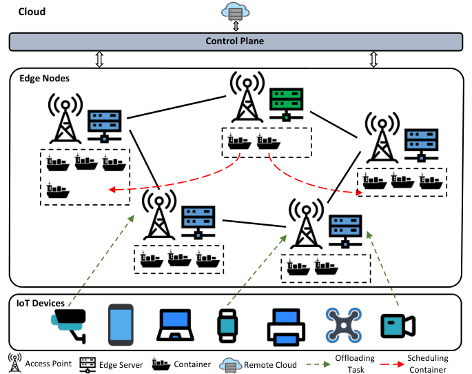
We model a one-round upgrade scenario for an edge cluster. As illustrated in Fig. 1, computation-intensive tasks from IoT devices are offloaded to edge nodes, where the results are processed and returned. Tasks are executed in containers, which require the corresponding image to be pulled locally before execution. Upgrades may occur periodically due to security patches, bug fixes, etc. [8, 9]. The cluster adopts a rolling upgrade strategy, in which all nodes in the cluster upgrade sequentially, with the node being upgraded shown in green and the node not being upgraded in blue. To ensure uninterrupted service, all containers on a node must be scheduled to another node before upgrading. During the upgrade, new tasks are continuously offloaded to edge nodes, requiring decisions to be made regarding which node they are scheduled on. Meanwhile, resources in edge nodes are limited, and containers cannot be scheduled on nodes that do not meet resource requirements. Additionally, the node being upgraded is set as unschedulable.
The set of nodes is defined as , where indicates the number of elements in the set, e.g., represents the number of nodes. The set of tasks offloaded by different IoT devices to the edge node is . The set of images is denoted as , with each image associated with a container. We assume that the resources requested by the task are the same as those occupied by the container, and requesting a container is equivalent to requesting the corresponding image. For ease of reference, the main notations used in this paper are summarized in Table I.
| Notation | Definition |
|---|---|
| N | Node set |
| node () | |
| CPU resource of node at time | |
| Memory resource of node at time | |
| Storage capacity of node at time | |
| CPU frequency of node | |
| Bandwidth of node | |
| Upgrade status of node at time | |
| K | Task set |
| task () | |
| CPU request of task | |
| Memory request of task | |
| CPU frequency request of task | |
| Image request of task | |
| Size of task | |
| Image set | |
| Size of image |
II-B Latency
Communication latency. In the communication model, all IoT devices equally share the bandwidth of nodes. The uplink wireless transmission rate from task to node is defined as [16]:
| (1) |
where is the bandwidth of node and is the number of tasks transmitted to node at the same time. is the transmission power, is the channel gain between the IoT device and the node, and represents the power of Gaussian white noise. The communication latency of task transmitted to node can be defined as follows:
| (2) |
Furthermore, similar to many studies [17, 18], we ignore the return communication latency of the result because the result is small compared with the task itself.
Download latency. Download latency refers to image download latency, which is defined as:
| (3) |
where is the image requested by task and is the size of the image required to process task . is the binary variable to indicate whether image is on node . If , image is on node , otherwise not on node . is the queuing download latency on node . Therefore, if the image required to process the task is available locally, the download latency is 0.
Computation latency. Different tasks are executed in different containers, and all tasks are executed in parallel. The computation latency can be calculated as follows:
| (4) |
where is the CPU frequency requested by task , and is the computing power of node .
In summary, the total latency of task execution on node can be denoted as:
| (5) |
II-C Problem Formulation and Analysis
Constraints. The containers need to be assigned certain resources, while the total amount of resources on the node is limited. The resource limits on the node can be denoted as:
| (6) |
where the binary variable indicates whether task is executed on node . If , the task is executed on node . Otherwise, the task is not executed on node .
Meanwhile, the storage space for the image on a node is limited, which can be defined as:
| (7) |
Furthermore, tasks are regarded as indivisible, so each task is scheduled to only one node, which can be expressed as:
| (8) |
Problem Formulation. We aim to minimize the average total latency of the tasks during the edge cluster upgrade. The target is to find the best policy to minimize the latency while obeying the constraints. The OCS problem is defined as:
Problem OCS.
| (9) | ||||
The OCS problem is NP-hard, so the traditional algorithm may need help to get the optimal solution in a reasonable time. The RL algorithm can gradually lead to a better solution through continuous learning and optimization [19].
III Algorithms
In this section, the settings of the OCS algorithm are first presented. Then, the OCS algorithm is illustrated.
III-A Algorithm Settings
In this subsection, the settings in the RL algorithm are introduced, including state, action space, and reward.
State. The state contains the node state and task state. The node state includes the resource state and the upgrade state. The resource state includes the CPU, memory, and storage capacity of the node at time , as well as the CPU frequency and bandwidth of the node, which can be defined as:
| (10) | ||||
The upgrade status of the node at time is denoted by the variable . indicates that node has not been upgraded, indicates that node is being upgraded, and indicates that node has been upgraded. Therefore, the upgrade state of nodes can be denoted as:
| (11) |
Finally, the state for all nodes is defined as follows:
| (12) |
The task state includes the status of the images required to execute the task on each node and the requested resources. Thus, the task state can be denoted as follows:
| (13) | ||||
where is the download time of the image in each node, which can be calculated by Eq. (3).
In summary, the state at time is defined as:
| (14) |
Action space. The container used to execute tasks is scheduled by the scheduler. The OCS algorithm needs to determine which node to schedule. Therefore, the action space is the set of all nodes as follows:
| (15) |
Reward. Defining a proper reward is crucial in the RL algorithm. Since different tasks require varying amounts of computation power, considering only the total latency may lead to an unstable training process. Thus, both the expected and actual latencies of the task are included in the reward, which can be defined as follows:
| (16) |
where represents the expected total latency of the task, and denotes the minimum value of the node CPU frequency. If the task is completed earlier than expected, the reward is positive, with the completion time being inversely proportional to the reward. Conversely, the reward is smaller. From a long-term perspective, the cumulative reward is , where is the discount factor with a value ranging between [0, 1].
III-B Online Container Scheduling
Overview. The OCS algorithm considers the heterogeneity of edge nodes and the characteristics of tasks in the edge cluster. The framework of the OCS algorithm is depicted in Fig. 2. Specifically, the node state and task state can be observed from the environment. After obtaining their features, they are embedded and concatenated, and then fed into the policy network to make the corresponding scheduling operations. The reward is subsequently obtained based on the action. Finally, the policy network and value functions are updated using the policy gradient-based algorithm.
Training. The OCS algorithm is based on policy optimization. Policy gradient [20] is an RL algorithm that directly optimizes the expected return policy. Let denote a policy with parameters . The Proximal Policy Optimization (PPO) algorithm [21] is based on the policy gradient algorithm, which ensures effectiveness with low computational complexity. The optimization objective of PPO is as follows:
| (17) |
and
| (18) | ||||
where is a clip function to limit to the range of and is a hyperparameter that represents the range of clips. Besides, PPO adopts the Generalized Advantage Estimator (GAE) [22] to compute the advantages, which can be calculated by:
| (19) |
where is the GAE parameter, is the TD-error at time step , and is an approximate value function.
The OCS algorithm is presented in Algorithm 1. The replay memory is first initialized for each episode. As shown in Lines 3 - 9, for each time slot , the observation state of the current time slot is first obtained, then the action is selected according to the policy, and the reward is calculated. Afterward, the next state is obtained. Finally, the transition is stored in the replay memory . As shown in Lines 10 - 14, for each training step , the advantage estimation is first computed based on the collected set of trajectories. Then, the stochastic gradient ascent algorithm with Adam is used to maximize the objective function to update the policy. Finally, the results are output after all episodes are completed.


IV Evaluation
In this section, we will delve into the performance of the OCS algorithm through simulation experiments.
IV-A Experimental Settings
Parameter settings. Similar to [23, 16], we set the transmission power and the noise power spectrum density . According to the physical interference model [24], the channel gain between the IoT device and the node is set to , where is the distance between the IoT device and the node and is the path loss factor. The communication bandwidth between the IoT device and the node is set to [100, 200] Mb/s.
The area of the simulation region increases as the number of nodes increases, and the default area is . All nodes are heterogeneous and randomly distributed, and the default number of nodes is 15. The CPU capacity of the node is set between [80,120] cores. The CPU frequency is set between [15,35] GHz, and the memory is set between [70,130] GB. The task is randomly generated in the simulation region, and the task sizes are set from 10 KB to 10 MB. The types of requested images follow the normal distribution. The hyperparameters of the OCS algorithm are listed in TABLE II.
| Type | Hyperparameter | Value |
|---|---|---|
| Actor | Hidden layers | 2 Full connection (128,64) |
| Learning rate | 1e-4 | |
| Critic | Hidden layers | 2 Full connection (128,64) |
| Learning rate | 3e-4 | |
| Other | Discount factor | 0.98 |
| GAE parameter | 0.95 | |
| Clipping threshold | 0.2 | |
| Batch size | 32 | |
| Optimizer | Adam |
Baselines. We compare the OCS algorithm with several baseline algorithms to demonstrate the effectiveness of our proposed algorithm: (1) EQ. EqualPriority (EQ) sets the weight of all nodes to 1. (2) RB. ResourcesBalanced (RB) prioritizes balancing the resource usage of each node. (3) LA. LeastAllocated (LA) is a scheduling policy related to the resource usage of the node. (4) IL. ImageLocality (IL) considers the local existence of the image requested by the task. These baselines are built-in scheduling policies in Kubernetes. Moreover, LA and IL are greedy algorithms that select nodes with more resources or images.
IV-B Experimental Results
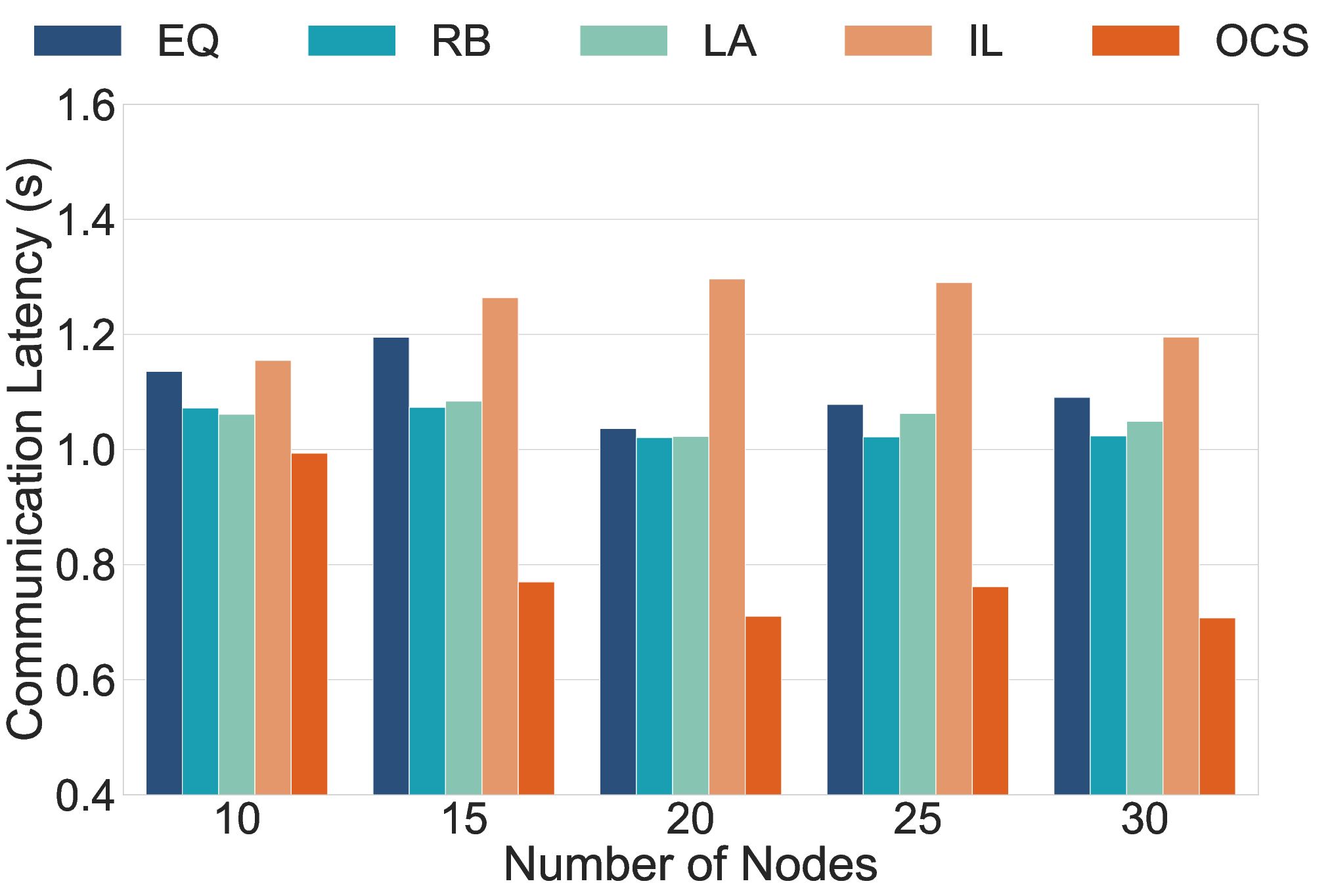
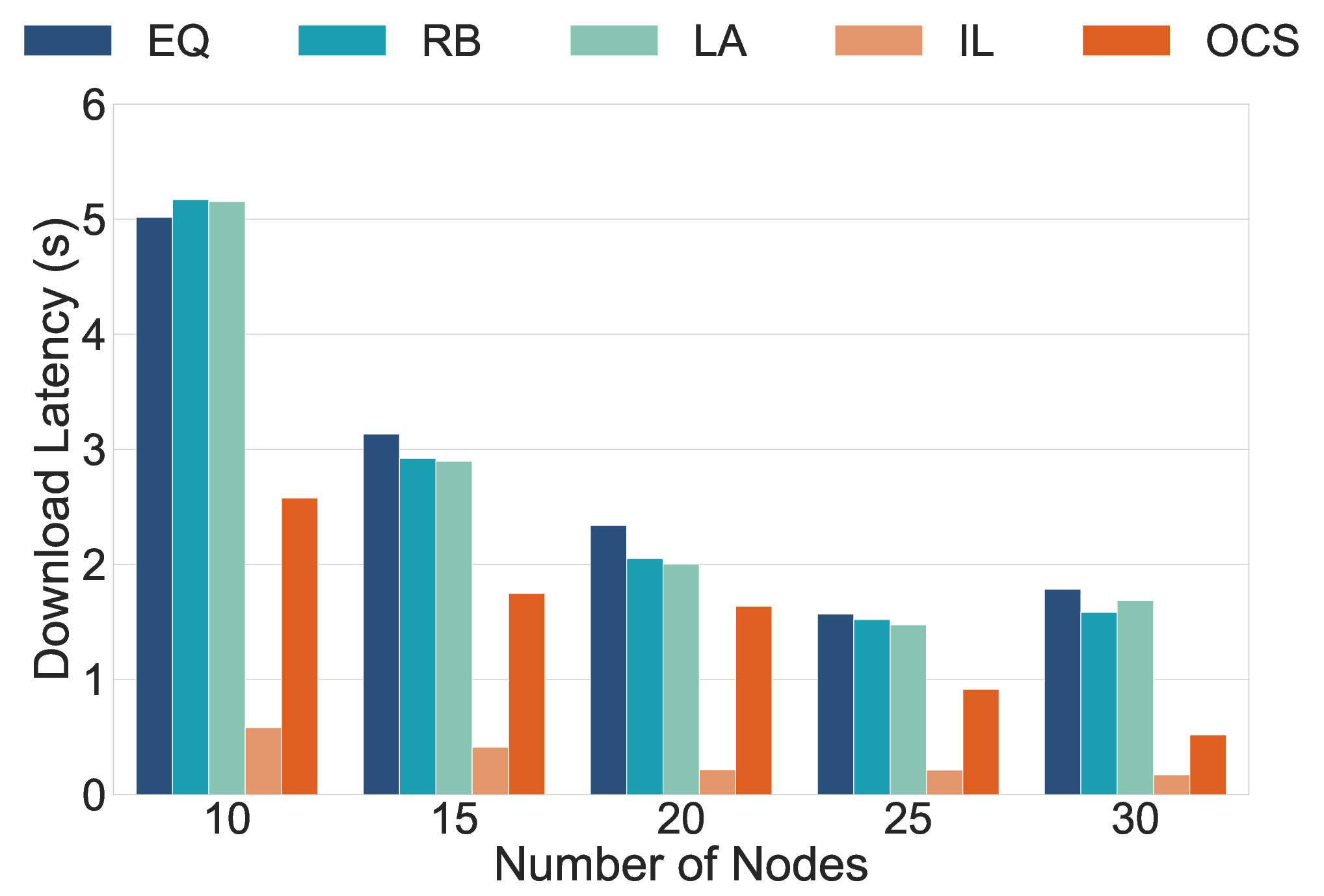
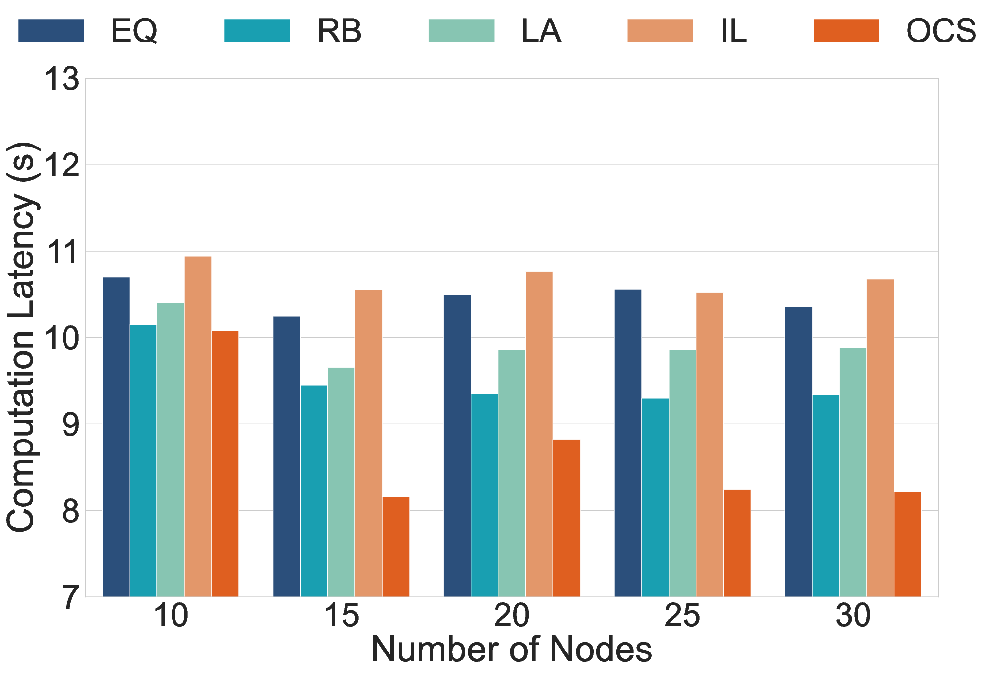
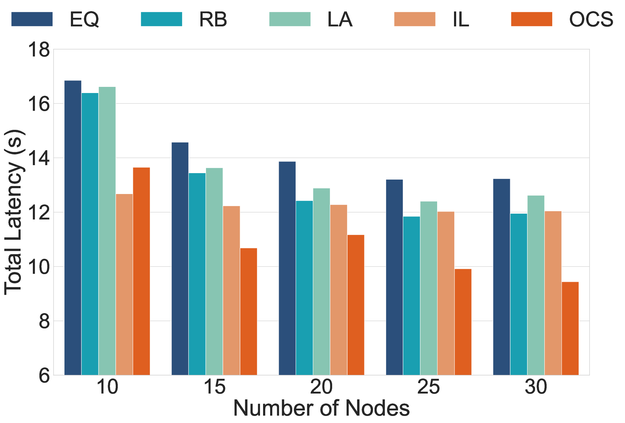
Performance with different numbers of nodes. Fig. 3 shows the average total latency as the number of nodes increases, including communication latency, download latency, computation latency, and total latency. As seen from this figure, the average latency of tasks decreases as the number of nodes increases. The reason is that more nodes are available for scheduling as the number of nodes increases. The scheduler can schedule the containers to more suitable nodes, such as those with a closer distance or more resources. As a result, the average total latency of the task becomes smaller. On the whole, the total latency relationship is OCS IL RB LA EQ. Therefore, the OCS algorithm performs the best regardless of the number of nodes. Specifically, the total latency with different numbers of nodes is reduced by 40%, 33%, 27%, and 26% on average compared with EQ, LA, RB, and IL algorithms, respectively.
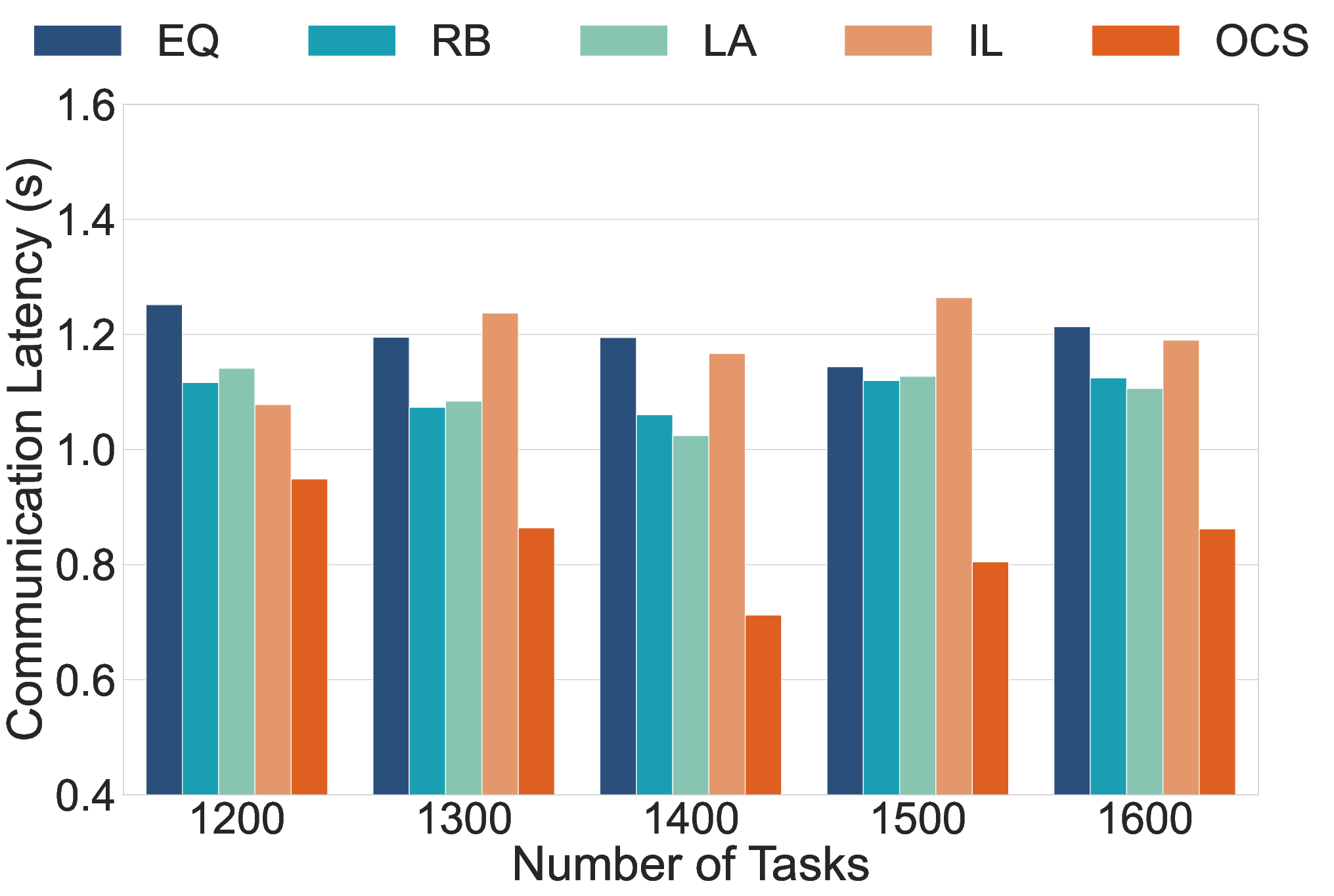
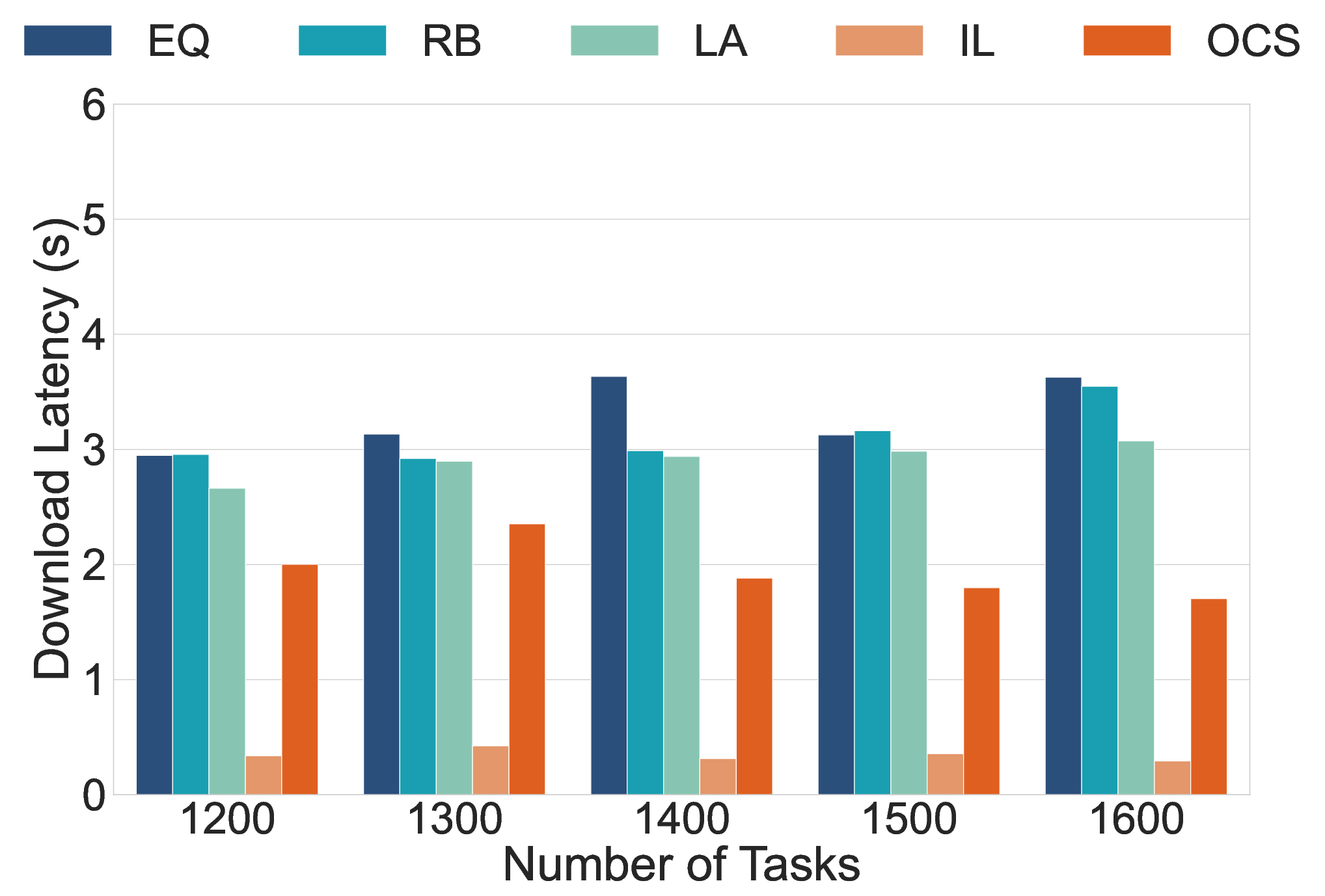
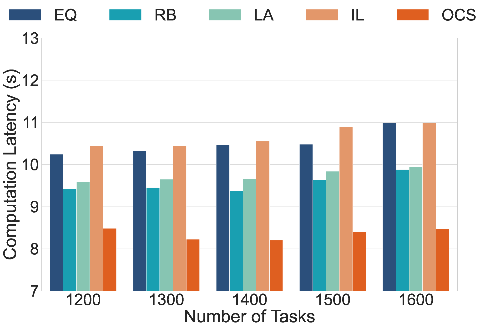
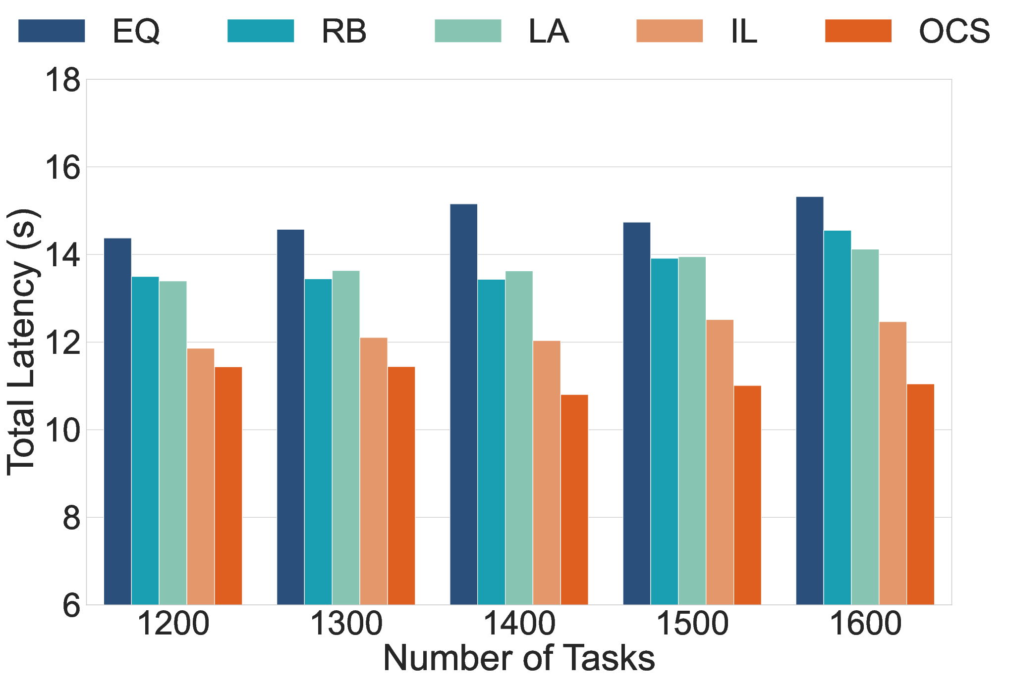
Performance with different numbers of tasks. The variation of average task latency as the number of tasks increases is illustrated in Fig. 4. The results indicate that the OCS algorithm performs best. While the IL algorithm performs slightly less, the RB and LA algorithms are very close, and the EQ algorithm performs the worst. Overall, as the number of tasks increases, the relationship between the performance of different algorithms in total latency is OCS IL LA RB EQ. Compared to the EQ, RB, LA, and IL algorithms, the total scheduling latency for the OCS algorithm is reduced by 38%, 31%, 27%, and 12%, respectively.
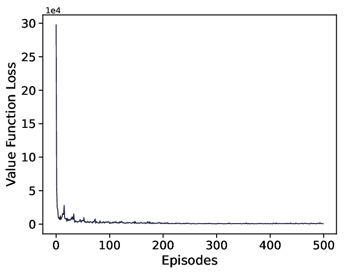
Performance of the OCS algorithm. Fig. 5 shows the convergence of the OCS algorithm. The policy network loss and value function loss of the OCS algorithm have large values at the beginning of training. However, as the training steps increase, both decrease rapidly and eventually fluctuate near a specific value, indicating that the algorithm has converged.
V Conclusion
This paper proposes a low-latency container scheduling algorithm for IoT services in edge cluster upgrades. First, we comprehensively model the OCS problem, considering communication, download, and computation latency. Second, a policy gradient-based RL algorithm is proposed to make online scheduling decisions, which fully considers the distinctive features of MEC. Finally, experiments are conducted on a simulated edge cluster, and the experimental results demonstrate that our algorithm achieves approximately 27% lower total latency compared to the baseline algorithm. In future work, we will deploy this algorithm in the Kubernetes system.
Acknowledgment
This work is supported in part by the Guangdong Key Lab of AI and Multi-modal Data Processing, United International College (UIC), Zhuhai under Grant 2020KSYS007 sponsored by Guangdong Provincial Department of Education; in part by the Chinese National Research Fund (NSFC) under Grant 62272050; in part by Institute of Artificial Intelligence and Future Networks (BNU-Zhuhai) and Engineering Center of AI and Future Education, Guangdong Provincial Department of Science and Technology, China; Zhuhai Science-Tech Innovation Bureau under Grants ZH22017001210119PWC and 28712217900001, and in part by the Interdisciplinary Intelligence SuperComputer Center of Beijing Normal University (Zhuhai).
References
- [1] L. Qian, Y. Wu, F. Jiang, N. Yu, W. Lu, and B. Lin, “Noma assisted multi-task multi-access mobile edge computing via deep reinforcement learning for industrial internet of things,” IEEE Transactions on Industrial Informatics, vol. 17, no. 8, pp. 5688–5698, 2020.
- [2] L. Toka, G. Dobreff, B. Fodor, and B. Sonkoly, “Machine learning-based scaling management for kubernetes edge clusters,” IEEE Transactions on Network and Service Management, vol. 18, no. 1, pp. 958–972, Mar. 2021.
- [3] T. Goethals, F. De Turck, and B. Volckaert, “Extending kubernetes clusters to low-resource edge devices using virtual kubelets,” IEEE Transactions on Cloud Computing, vol. 10, no. 4, pp. 2623–2636, Oct. 2022.
- [4] L. Ma, S. Yi, N. Carter, and Q. Li, “Efficient live migration of edge services leveraging container layered storage,” IEEE Transactions on Mobile Computing, vol. 18, no. 9, pp. 2020–2033, Sep. 2019.
- [5] S. Wang, Y. Guo, N. Zhang, P. Yang, A. Zhou, and X. Shen, “Delay-aware microservice coordination in mobile edge computing: A reinforcement learning approach,” IEEE Transactions on Mobile Computing, vol. 20, no. 3, pp. 939–951, Mar. 2021.
- [6] Z. Tang, J. Lou, and W. Jia, “Layer dependency-aware learning scheduling algorithms for containers in mobile edge computing,” IEEE Transactions on Mobile Computing, 2022, doi: 10.1109/TMC.2021.3139995.
- [7] Google. Kubernetes. [Online]. Available: https://kubernetes.io/
- [8] H. Guissouma, H. Klare, E. Sax, and E. Burger, “An empirical study on the current and future challenges of automotive software release and configuration management,” in 2018 44th Euromicro Conference on Software Engineering and Advanced Applications (SEAA). IEEE, 2018, pp. 298–305.
- [9] A. Decan, T. Mens, A. Zerouali, and C. De Roover, “Back to the past–analysing backporting practices in package dependency networks,” IEEE Transactions on Software Engineering, vol. 48, no. 10, pp. 4087–4099, 2021.
- [10] L. E. Lwakatare, T. Kilamo, T. Karvonen, T. Sauvola, V. Heikkilä, J. Itkonen, P. Kuvaja, T. Mikkonen, M. Oivo, and C. Lassenius, “Devops in practice: A multiple case study of five companies,” Information and Software Technology, vol. 114, pp. 217–230, 2019.
- [11] A. Alsharif, C. W. Tan, R. Ayop, K. Y. Lau, and A. Moh’d Dobi, “A rule-based power management strategy for vehicle-to-grid system using antlion sizing optimization,” Journal of Energy Storage, vol. 41, p. 102913, 2021.
- [12] A. Mehrabi, M. Siekkinen, and A. Ylä-Jääski, “Edge computing assisted adaptive mobile video streaming,” IEEE Transactions on Mobile Computing, vol. 18, no. 4, pp. 787–800, 2018.
- [13] X. Hu, C. Masouros, and K.-K. Wong, “Reconfigurable intelligent surface aided mobile edge computing: From optimization-based to location-only learning-based solutions,” IEEE Transactions on Communications, vol. 69, no. 6, pp. 3709–3725, 2021.
- [14] J. Chen, Y. Yang, C. Wang, H. Zhang, C. Qiu, and X. Wang, “Multitask offloading strategy optimization based on directed acyclic graphs for edge computing,” IEEE Internet of Things Journal, vol. 9, no. 12, pp. 9367–9378, 2021.
- [15] R. S. Sutton and A. G. Barto, “Reinforcement learning: An introduction,” IEEE Transactions on Neural Networks, vol. 16, pp. 285–286, 2005.
- [16] Y. Wang, X. Tao, X. Zhang, P. Zhang, and Y. T. Hou, “Cooperative task offloading in three-tier mobile computing networks: An admm framework,” IEEE Transactions on Vehicular Technology, vol. 68, no. 3, pp. 2763–2776, Mar. 2019.
- [17] M. Chen and Y. Hao, “Task offloading for mobile edge computing in software defined ultra-dense network,” IEEE Journal on Selected Areas in Communications, vol. 36, no. 3, pp. 587–597, Mar. 2018.
- [18] J. Du, L. Zhao, J. Feng, and X. Chu, “Computation offloading and resource allocation in mixed fog/cloud computing systems with min-max fairness guarantee,” IEEE Transactions on Communications, vol. 66, no. 4, pp. 1594–1608, Apr. 2018.
- [19] H. Wang, T. Zariphopoulou, and X. Y. Zhou, “Reinforcement learning in continuous time and space: A stochastic control approach,” The Journal of Machine Learning Research, vol. 21, no. 1, pp. 8145–8178, 2020.
- [20] R. S. Sutton, D. McAllester, S. Singh, and Y. Mansour, “Policy gradient methods for reinforcement learning with function approximation,” in Advances in Neural Information Processing Systems, vol. 12. MIT Press, 1999.
- [21] J. Schulman, F. Wolski, P. Dhariwal, A. Radford, and O. Klimov, “Proximal policy optimization algorithms,” Aug. 2017.
- [22] J. Schulman, P. Moritz, S. Levine, M. Jordan, and P. Abbeel, “High-dimensional continuous control using generalized advantage estimation,” arXiv preprint arXiv:1506.02438, 2015.
- [23] X. Chen, “Decentralized computation offloading game for mobile cloud computing,” IEEE Transactions on Parallel and Distributed Systems, vol. 26, no. 4, pp. 974–983, Apr. 2015.
- [24] A. Goldsmith, Wireless communications. Cambridge University Press, 2005.