Training Latency Minimization for Model-Splitting Allowed Federated Edge Learning
Abstract
To alleviate the shortage of computing power faced by clients in training deep neural networks (DNNs) using federated learning (FL), we leverage the edge computing and split learning to propose a model-splitting allowed FL (SFL) framework, with the aim to minimize the training latency without loss of test accuracy. Under the synchronized global update setting, the latency to complete a round of global training is determined by the maximum latency for the clients to complete a local training session. Therefore, the training latency minimization problem (TLMP) is modelled as a minimizing-maximum problem. To solve this mixed integer nonlinear programming problem, we first propose a regression method to fit the quantitative-relationship between the cut-layer and other parameters of an AI-model, and thus, transform the TLMP into a continuous problem. Considering that the two subproblems involved in the TLMP, namely, the cut-layer selection problem for the clients and the computing resource allocation problem for the parameter-server are relative independence, an alternate-optimization-based algorithm with polynomial time complexity is developed to obtain a high-quality solution to the TLMP. Extensive experiments are performed on a popular DNN-model EfficientNetV2 using dataset MNIST, and the results verify the validity and improved performance of the proposed SFL framework.
Index Terms:
Federated learning, split learning, edge computing, computing task offloading, resource allocation.I Introduction
The latest Artificial Intelligence (AI) products are powered by cutting-edge machine learning (ML) technology, ranging from face detection [1] and speech recognition [2] installed on mobile devices to virtual assistants deployed in autonomous systems [3]. Large-scale data is essential for training high-performance AI-models, e.g., decision trees, support vector machines (SVMs), and deep neural networks (DNNs). However, centralized approach to training AI-models requires clients to transfer privately-owned data to servers, which poses a great threat to users’ privacy and security [4]. Google has proposed a new ML paradigm, called federated learning (FL) [5], that allows multiple clients to train an AI-model in a distributed manner, while keeping their data local. The vanilla FL algorithm, called FedAvg is illustrated in Fig. 1 (the left part). A parameter server (PS) first distributes an AI-model to be trained to multiple selected clients. Then, each client trains the model locally with the relevant data and upload the trained model to the PS for aggregation. This process is iterated for several rounds and the aggregated model achieves a certain test accuracy.
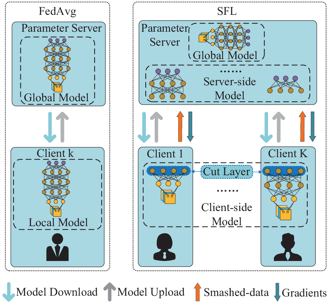
However, FedAvg is more suitable for training lightweight AI-models, where the communication cost is greater than the computational cost caused to clients [5]. With the rapid popularization of high-speed mobile communications (such as 5G) and the development of large-scale deep AI-models (such as DNNs), the application context of FL has undergone fundamental changes:
- •
The ultra-reliable and low-latency communication technologies of 5G make the communication cost no longer the bottleneck for FL [6].
- •
The computing power of mobile devices has not been improved significantly, compared with the rapidly growing demand for training large-scale DNN-models [7].
New techniques and methods are needed to cope with the new trends in the development of AI-models.
Fortunately, the method of split learning (SL) [8] supported by edge computing [8] provides a feasible solution to the above challenges. As illustrated in Fig. 1 (the right part), the model-split allowed FL (SFL) first splits an AI-model into two parts, which can be trained separately [4]. The part trained by the client is called the client-side model, while the other part trained by the PS is called the server-side model. The client initiates the forward propagation (FP) on the client-side model to obtain the intermediate result, called the smashed-data, and then, uploads it to the PS. The PS uses the received smashed-data as the input to continue the FP on the server-side model. Thereafter, the PS can initiate the backward propagation (BP) on the server-side model. The obtained gradients, as the server-side intermediate result, is transferred to the client, so the client can use it to complete the BP on the client-side model.
Notably, by equipping the PS with a high-performance computing server, it can then process multiple server-side models (offloaded by multiple clients) in parallel, thus greatly reducing the computational burden of the clients. However, unlike in FedAvg, the clients in SFL cannot independently perform the FP and BP, resulting in the intermediate results being communicated hundreds of times during training client-side models. The reduced computational burden on clients may lead to the increased network data traffic. Although this fits the trend of increased network bandwidth and larger-and-deeper AI-models, the following issues must be addressed in order to improve the training efficiency of SFL:
Challenge 1: Cut-layer selection of the clients. In the paradigm of SL, the cut-layer for a client refers to the last layer of the client-side model [9], as shown in Fig. 1. The client-selected cut-layer determines its communication load (for transmitting the smashed data) and computational load (for training the client-side model). However, there is no explicit relationship between the cut-layer and other parameters of an AI-model, which brings to a client a huge discrete solution space and extremely high computational complexity to choose the optimal cut-layer.
Challenge 2: Computing resource allocation of the PS. In SFL, a PS can simultaneously train multiple server-side models offloaded by the participating clients. Due to the heterogeneity of clients in computing power and datasets, the PS must optimize its allocation of the limited computing resources to improve the training efficiency of SFL.
In this paper, we leverage edge computing and split learning to improve the training efficiency of SFL. In particular, we aim to minimize the training latency of the SFL using synchronized global model update (SGMU) [10] without losing the test accuracy of the trained model. Under the SGMU setting, the latency in completing a round of global training is determined by the maximum latency for the participating clients to complete a session of local training. Therefore, the training latency minimization problem (TLMP) is modelled as one that minimizes the maximum latency for the clients to complete a local training session. To address Challenge 1 inherent in the problem, we take a popular AI-model, EfficientNetV2 [11], as an example and propose a regression method to fit the quantitative relationship between the cut-layer of the trained model and the resulting communication and computational loads for a client. Then, the original mixed integer nonlinear programming (MINLP) problem is transformed into a continuous one. Considering the relative independence of cut-layer selection and computing resource allocation, this problem is further decoupled into two subproblems, namely, the cut-layer selection problem of the clients (to address Challenge 1) and the computing resource allocation problem of the PS (to address Challenge 2). Finally, an alternate-optimization-based algorithm is proposed to obtain a high-quality solution to the training latency minimization problem. Extensive experiments are performed on EfficientNetV2 using dataset MNIST [12], and the results verify the validity of our proposed method.
In summary, the main technical contributions of this paper are as follows:
- 1.
The edge computing and split learning techniques are orchestrated to improve the training efficiency of SFL. With the specific aim to minimize the training latency of the SFL using SGMU without loss of test-accuracy, an MINLP problem, called the TLMP, is formulated. The TLMP achieves the goal by constantly removing the system bottleneck, i.e., the maximum latency for the participating clients to complete a local training session.
- 2.
To address Challenge 1 inherent in the TLMP, a regression method is presented to fit the quantitative relationship between the cut-layer of an AI-model and the communication and computational loads generated to a client. In this way, the original MINLP problem is transformed into a continuous one.
- 3.
By decoupling the continuous TLMP into two independent subproblems, namely, the cut-layer selection problem of the clients and the computing resource allocation problem of the PS, an alternate-optimization-based algorithm with polynomial time complexity is designed to obtain a high-quality solution to the original TLMP. Extensive experiments testify the effectiveness of the proposed method.
The rest of this paper is organized as follows. Sec. II reviews the related works. Sec. III describes the detailed training procedure of the SFL using SGMU. Sec. IV first gives the parameterized expressions for the time consumption of the SFL, and then, formulates the TLMP as a min-max problem. The algorithm to solve the TLMP is developed in Sec. V. In Sec. VI, experiment results are provided to verify the effectiveness of the proposed method. Finally, the paper is summarized in Sec. VII.
II Related Works
Federated Learning: As an effective distributed machine learning method for privacy protection, FL has been widely studied and applied in many fields. Parameter Server architecture [13] is widely used to enable a large number of computation nodes to train a shared model by aggregating locally-computed updates. Federated optimization [14] is proposed in to improve communication efficiency by minimizing communication rounds, while keeping training data local and protecting data privacy. To make FL more practical, an effective client selection algorithm is proposed in [15] to solve the straggler (clients requiring longer training times) problem. Issues of fairness assurance between participating clients were discussed in [16]. In [17], the authors counterbalanced the bias introduced by non-IID data and accelerated the convergence of model training. In [18], local training of clients constrained by computing power is accelerated by training task offloading. In [19], the authors studied the non-convex resource allocation problem of FL over wireless networks.
Splitting Learning : Distributed training of large-scale AI-models requires large amount of computing resources, but the limited computing resources of clients become the bottleneck restricting the performance (e.g., training latency, test accuracy, etc.) of FL. Thereby, some recent researches focus on reducing the computational burden of clients. Split learning (SL) [20] is one of the methods, which can divide an AI-model into multiple parts and trains them separately in a certain order. A parallel SL method is proposed in [21] to prevent overfitting due to differences in the training order and data size of the segmented model parts. In [22], the authors use SL to assist the collaborative computation of DNNs between mobile devices and cloud server, and formulate the optimal computing-resource scheduling problem for the DNN layers as the shortest path problem and integer linear programming. In [23], the authors proposed a multi-split algorithm that can assign DNN submodels to each computational node in a given network topology, and a computational graph search problem was proposed to optimize the assignment. In [24], SL is used to reduce the total energy cost of edge devices under time-varying wireless channels. In [25], the coexistence of FL and SL is allowed in wireless networks, and the convergence of hybrid split and federated learning (HSFL) algorithm is analyzed with non-IID data distribution.
Collaborative training of AI-models: In a collaborative training framework such as FL, the bottleneck is in the computing power and workload differences between the client and the edge server. Therefore, some recent studies have focused on the allocation of computing, storage and communication resources for edge devices to improve the efficiency of collaborative training. To eliminate the straggler clients in an FL task, a timeout threshold is set in [26], after which the uploaded model will be discarded to reduce the overall training latency. An effective method is proposed in [27] to dynamically and virtually allocate the computing and communication resources of an edge server to multiple clients, allowing the task offloading of the clients. The challenge lies in estimating client training time, as the real time consumption is only known after the actual run. To address this issue, the data fitting method, i.e., optimal regression model, is proposed in [9] to predict training time of clients. The authors in [16] modelled the estimation of client’s local time consumption (consisting of transmitting and training model) as a C2MAB problem. Then, they converted the online scheduling problem into an offline problem with Lyapunov optimization and solved it using a divide-and-conquer method. By applying deep reinforcement learning (DRL), a capability-matched model offloading strategy is designed in [10] for heterogeneous clients, aiming to minimize the training latency of an FL task. The authors in [28] used DNN partitioning to minimize the FL training latency under the constraints of device-specific participation rates, energy consumption, and memory usage, regardless of the transmission of the smashed data over a wireless network.
Summary: Inspired by the existing works, we leverage edge computing and SL to improve the training efficiency of FL, a collaborative training paradigm. Under the synchronized global model update (SGMU) setting, the two key challenges described in Sec. I, namely, (1) cut-layer selection of the clients and (2) computing resource allocation of the PS, must be dealt with jointly, which is not yet involved in the related works.
III System Model
We consider a FL system consisting of a unique PS and a set of clients. The goal of the PS is to train an AI-model with the data owned by the clients but without directly sharing the data. Next, we review FedAvg, the vanilla FL algorithm, and then, describe SFL, the edge computing and split learning supported FL method. The system parameters are summarized in the following Table I.
| Symbol | Description |
|---|---|
| , , | Local model of client , client-side model of client , server-side model of client . |
| , | Local dataset of client , mini-batch of client . |
| , , | The sample of or , ground-true label, prediction of the label. |
| , | Sample-wise loss function, gradient of loss function. |
| Learning rate. | |
| Number of epochs in a local training session of client . | |
| The parameters of the layer of model w. | |
| The number of layers of an AI-model. | |
| , | Cut-layer of client , the minimum value of that client can take. |
| Sample-wise smashed-data of client . | |
| Sample-wise gradients of client . | |
| Size of and . | |
| Data rate between the PS and client . | |
| Computing power of client for training . | |
| Computing power of the PS allocated to client for training . | |
| , | Amount of computing resources required for client to perform FP/BP with one data-sample. |
| , | Amount of computing resources required for the PS to perform FP/BP with one data-sample. |
| , which is the computational load of client for training the client-side model. | |
| Amount of computing resources required to train an AI-model with one data-sample. | |
| Amount of computing resources available for the PS. | |
| Latency for client to complete a local training session. | |
| Latency for the clients to complete a round of global training. | |
| L | . |
| F | . |
| Latency for client to complete a local training session using only the local computing power . | |
| New index of client according to . | |
| Set of clients adopting FedAvg to train the local model. | |
| Set of clients adopting SFL to train the local model. | |
| The index of the first client in . |
III-A The Basic of FedAvg
In FedAvg [5], the PS first broadcasts the initial model w to the clients. Then, each client () trains the model, represented by , locally and independently by using its own dataset , where is the size of the dataset, and and are respectively the sample and its ground-true label.
Local training at client k: Using the stochastic gradient descent (SGD), a mini-batch can be randomly sampled from to train in each local training epoch. With each , client first performs the FP to obtain , the prediction of using the current model . Then, client performs the BP and calculates the gradient w.r.t , where is the sample-wise loss function. The local model of client can be updated as
| (1) |
where is the learning rate.
During a local training session, the above training epoch is iterated times. Thereafter, client uploads the trained model to the PS for aggregation.
Global model update at the PS: Under the synchronized global model update (SGMU) setting, the PS can update the global model w by using the following eq. (2), only if all the local models of the clients are collected.
| (2) |
The global model update will be iterated several rounds until the learning goal (e.g., a certain prediction accuracy on the test dataset or the maximum number of global training rounds) is achieved.
III-B The Framework of SFL
Referring to [9], a layer of an AI-model is defined as the minimum divisible unit of the model parameter, which can be either a separate layer (for example, active, convolution, or fully connection layers) or a combination of multiple consecutive layers. Then, an AI-model w can be partitioned into layers as
| (3) |
where represents the layer’s parameter of the model and the operator represents connecting any two consecutive layers.
Unlike FedAvg, which orders each client to train independently, SFL splits for each client into the following two parts
| (4) |
where and are respectively called the client-side model and server-side model, and are respectively submitted to client and the PS for training. The last layer of the client-side model, , is termed as the cut-layer for client [29].

In Fig. 2, we show the workflow of SFL, which includes the following 5 phases: 1) Splitting local models; 2) Distributing local models; 3) Training local models; 4) Collecting local models; and 5) Aggregating local models. The main difference between SFL and FedAvg is in the and phases. The detail is given below.
Phase 3 (Training local models): Since is split into two parts, namely and , the training of requires the collaboration between client and the PS.
- •
Forward Propagation:
- (1)
Client-side FP: In each local training epoch, client starts the FP on the client-side model using mini-batch . The output at the cut-layer , called the smashed-data [9], is given as
(5) - (2)
Uploading smashed data: Client uploads the smashed data and the label 11 1 Uploading labels to PS undermines the data-privacy of clients. To address this issue, the authors in [30] proposed a three-stage SL method to avoid the leakage. For reconstruction attacks on training data, the leakage risk can also be reduced by using the differential privacy [31][32]. This paper uses an approach similar to [9] that allows a client to independently select the minimum cut-layer to implement its security requirement. Please refer to eq. (17) and its description in Sec. IV-B for detail. as the client-side intermediate results, to the PS for further processing.
- (3)
Server-side FP: Upon receiving and , the PS continues the FP on the server-side model , and obtains the predicted value of as
(6)
- (1)
- •
Backward propagation:
- (4)
Sever-side BP: With and , the PS instead of client starts the BP. The server-side model is updated as
(7) - (5)
Downloading gradients: Let denote the gradients generated at layer , the first layer of . The PS should transfers as the server-side intermediate results to client to continue the BP.
- (6)
Client-side BP: Upon receiving from the PS, client can complete the client-side BP and updates the client-side model as
(8)
- (4)
Phase 5 (Aggregating local models): At the end of each local training session, client uploads the trained client-side model to the PS. The PS can then combine with the trained server-side model as . Under the SGMU setting, when obtaining all of the clients, the PS can aggregate them to update the global model w by using eq. (2).
IV Problem Formulation
Although the SFL reduces the computational burden of clients for training local models, the communication overhead inevitably increases because the intermediate results and are communicated multiple times between the PS and each client due to the collaborative training.
In this section, we first quantify the latency of each phase of the SFL. Then, the training latency minimization problem is proposed.
IV-A Latency of each phase
Referring to Sec. III-B, the latency of each phase of the SFL is analyzed as follows.
Phase 1 (Splitting local models): The latency of this phase is caused by performing Algorithm 1, namely, the joint cut-layer selection and computing resource allocation algorithm proposed in Sec. V-E. Considering that the algorithm has a polynomial time complexity and runs on the PS with sufficient computing power, the latency is negligible.
Phase 2 (Distributing local models): Let denote the data rate between the PS and client in the current round of global training 22 2 In general, the uplink bandwidth and downlink bandwidth are asymmetric. Since the intermediate results generated by the clients are different, in the downlink, PS can only distribute the intermediate results to the clients using orthogonal unicast rather than broadcast. So we assume that the uplink and downlink rate is the same for each client.. The latency for client to download the client-side model from the PS is given by
| (9) |
where denotes the size (in bits) of .
Phase 3 (Training local models): As analyzed in Sec. III-B, the training of the local model of any client , , consists of 6 stages. The latency of each stage is given below.
- (1)
Client-side FP. Let denote the number of float point operations (Flops) required for client to perform the sample-wise FP on . Let (in Flops/s) denote the available computing power for client . Then, the latency to process the total samples is given by
(10) - (2)
Uploading smashed-data. Let denoted the size (in bits) of . The latency of transmitting the total pieces of smashed-data is given by33 3 To start the BP, the PS must have the label of each sample. The labels can be transferred by the clients to the PS along with the smashed-data. Since the size of labels is much smaller than the smashed-data, the transmission overhead is omitted here.
(11) - (3)
Server-side FP. Let denote the number of Flops required for the PS to perform the sample-wise FP on . Let (in Flops/s) denote the computing power allocated by the PS to client . Then, the latency of processing the total samples is given by
(12) - (4)
Server-side BP. Let denote the number of Flops required for the PS to perform the sample-wise BP on . Then, the latency of processing the total samples is given by
(13) - (5)
Downloading gradient. Let (in bits) denote the size of . Then, the latency of downloading the total gradients is given by
(14) - (6)
Client-side BP. Let denote the number of Flops required for client to perform the sample-wise BP on . The time required to process the total samples is given by
(15)
Phase 4 (Collecting client models): After local training epochs, client uploads the updated client-side model to the PS for aggregation. The latency is given by
| (16) |
Phase 5 (Aggregating local models): Aggregating client models requires only small computation effort. Since the PS has sufficient computing power, the latency is negligible.
IV-B Overall time consumption of SFL
In general, the smashed-data and gradients generated by processing one data-sample have the same size . The latency for client to complete a local training session, i.e., local training epochs, is given by
| (17) |
where is the minimum value of that client can take. The value of reflects the privacy requirement of client . The larger , the less likely it is to derive the raw information of the client from .
From eq. (17), we note that when the cut-layer is selected as , and . It means that client prefers to train the entire model locally, as in FedAvg. In this case, one can get
| (18) |
By substituting eq. (18) into eq. (17) , the latency for client to complete a local training session in this case is given by
| (19) |
where , are the size of model w (in bits) and total amount of computing load for one data-sample of model w.
IV-C Training Latency Minimization Problem
From eq. (17), we know that
- •
The latency for any client to train the model and communicate the intermediate results depends on the selected cut-layer ;
- •
While the PS is much more powerful than each of the clients, it needs to serve many clients at the same time, so its available computing resources are relatively limited.
Hence, the communication and computing resources of the clients and PS must be jointly scheduled to adapt to the cut-layers selected for the clients, so that the overall training latency of the SFL can be minimized.
Because we can only accurately predict the available computing resources and data rate for the clients and PS for a short time in the future [10], our goal is set to minimize , the latency to complete one round of global training. As the SGMU is adopted, the overall latency depends on , the maximum latency for the clients to complete a local training session. Let and . The training latency minimization problem for the SFL is formulated as
| (21) | ||||
| s.t. | (21.1) | |||
| (21.2) | ||||
| (21.3) | ||||
| (21.4) |
where constraint (.1) is the value space of the cut-layer for client , constraint (.2) limit the maximum amount of computing resources available for the PS to , constraint (.3) comes from eq. (4), which guarantees the model integrity after being split for any client , and constraint (.4) comes from the following fact.
Given the AI-model to be trained, the amount of computing resources required to train the model with one data-sample, represented as , and the amounts of computing resources required to perform the sample-wise BP and FP, respectively represented as () and (), are constants. Therefore, we have the following equation, i.e., constraint (.4).
| (22) |
Since both continuous variable F and discrete variable L are involved, problem (21) is a mixed integer nonlinear programming (MINLP) problem, which cannot be solved directly by using conventional methods. In what follows, we develop effective methods to address this problem.
V Solving the Problem
In problem (21), the size of the client-side model (), the computing resources needed to train the client-side model (), and the amount of generated intermediate results () all depend on the selected cut-layer for client . However, as shown in the following Figs. 3, 5, and 6, there is no explicit relationship between the cut-layer and other parameters of an AI-model. Since a DNN usually has hundreds of layers, this will lead to a unusually high time and space complexity to find the optimal cut-layers for the clients. To the best of our knowledge, there is currently no better way to address this issue. In this paper, we propose a regression method to quantify the relationship between the cut-layer and other parameters of a given AI-model. Based on that, a fast and effective method is developed to find the high-quality solution of problem (21).
It is worth noting that logistic regression and curve fitting methods have been widely used to address such relationship fitting problems. For example, in [33] and [34], the authors built practical non-linear energy harvesting models by curve fitting for measurement data. Based on the fitted model, effective resource allocation algorithms are developed for wireless information and power transfer (SWIPT) systems.
V-A Fit The Relationship Between The Parameters of An AI-model
Different AI-models have different neural network structures. To the best of our knowledge, there is currently no better way to obtain their relationship expression. In this paper, we use the popular AI-model EfficientNetV2[11] as an example and propose the regression method to fit the relationship between the cut-layer and other parameters of an AI-model.
V-A1 Client-side model size against different cut-layers
As shown in Fig. 3, with increasing , the increase of is not obvious at the beginning, but the growth rate increases sharply when . Therefore, we set the relationship between and as
| (23) |
where is the parameter to be fitted.

V-A2 Training load of client against different cut-layers
The training of the client-side model includes the FP and BP. The computational load of performing the FP can be obtained by using the python package torchinfo [35], however, there is no direct way to know the computational load of performing the BP. To address this issue, we trained EfficientNetV2 1500 times using a dataset of size 32. The time consumed by FP and BP in each training session is shown in Fig. 4.

From Fig. 4, we see that with the same computing power the time consumed by BP is roughly several times the time consumed by FP. So we have
| (24) |
where . Fig. 5 shows the computational load of client for training the client-side model (that is, ) with different cut-layers. There is an approximate linear relationship between them, which is given by
| (25) |
where is the parameter to be fitted.

V-A3 Size of intermediate results against different cut-layers
The head of a DNN is always a convolutional neural network (CNN) to extract features, thus reducing the computational burden of the subsequent feedforward neural network (FNN). Hence, the size of the intermediate results decreases rapidly in the CNN layers but changes slowly in the FNN layers, as shown in Fig. 6. Accordingly, we set the relationship between and as
| (26) |
where and are the parameters to be fitted.

V-B Problem Reformulation
By substituting eqs. (23), (25), and (26) into eq. (20), the expression for can be written as
| (27) |
Then, the MINLP problem (21) is transformed into the following continuous problem.
One can first find the solution of problem (28), and then, rounds it to an integer. We note that if the computing resource allocation F for the clients were known, problem (28) can be decomposed into independent subproblems, and the goal of the subproblem is to minimize the latency for client to complete a local training session. These subproblems can be solved in parallel without loss of optimality.
Based on the above findings, we can solve the cut-layer selection problem (to find the optimal L) and the computing resource allocation problem (to find the optimal F) alternately and iteratively. Finally, the solution to problem (28) can be obtained.
V-C Solving The Cut-Layer Selection Problem
For any given F, problem (28) can be decomped into independent subproblems as given below.
| (29) | ||||
| s.t. | (29.1) |
By solving problem (29), the optimal cut-layer of any client is obtained in closed-form, as shown in the following lemma.
Lemma 1.
With , the optimal cut-layer for any client is given by the following rules.
| (30) |
Proof.
Please refer to Appendix A. ∎
In the case of eq. (30), the function contains a cubic terms of and can be solved by using the Cardano’s formula [36]. It is worth noting that the complexity of finding the suboptimal cut-layers for the clients is only , thus avoiding an exhaustive search on the actual complex relationships between the parameters of an AI-model with extremely high time and space complexity.
V-D Computing Resource Allocation of the PS
Substituting the obtained cut-layers of the clients, namely, , into eq. (27), one can get
| (31) |
Problem (28) can be simplified to
| (32) | ||||
| s.t. | (32.1) |
The difficulty in solving problem (32) is that the objective, , to be optimized is a nonlinear function w.r.t , and is a piecewise function w.r.t . To solve this difficulty, we define as the latency for client to complete a local training session using only the local computing power . We can sort the clients in ascending order according to as shown in eq. (33), where the reordered index of client is represented as , .
| (33) |
Next, we derive the following two lemmas.
Lemma 2.
The clients participating in an FL task can be divided into two groups: the clients in group adopt FedAvg and train independently, while the clients in group adopt SFL and train in collaboration with the PS, where is the index of the first client in .
Proof.
Please refer to Appendix B. ∎
Lemma 3.
The optimum of the objective of problem (32) is , .
Proof.
Please refer to Appendix C. ∎
By using Lemmas 2 and 3, problem (32) can be converted into the following form.
| (34) | ||||
| s.t. | (34.1) | |||
| (34.2) | ||||
| (34.3) | ||||
| (34.4) |
By solving problem (34), the optimal amount of computing resources that the PS allocates to any client is obtained in closed-form, as shown in the following lemma.
Lemma 4.
The amount of computing resources allocated by the PS to each client is given by the following formula.
| (35) |
Proof.
Please refer to Appendix D. ∎
According to Lemma 4, once is known, the optimal resource allocation of the PS, F, can be obtained. In order to solve , we substitute formula (35) into constraint (.1) and convert this inequality constraint into an equality constraint as
| (36) |
Lemma 5.
is strictly convex w.r.t .
Proof.
Please refer to appendix E. ∎
V-E Algorithm Implementation and the Convergence and Complexity Analysis
In Step 8, function counts the number of non-zero elements in a vector. Since the algorithm contains iterative execution, the convergence is proved below.
Lemma 6.
Algorithm 1 converges to a stable point.
Proof.
For a feasible solution of problem (21), the resulting objective value can be obtained as .
In the iteration, the algorithm ensures that
| (37) | ||||||
| . |
Therefore, , the sequence of the objective values of problem (21), is non-increasing. Furthermore, because , the alternate-optimization-based algorithm can converge to a lower bound as the number of iterations increases. ∎
Finally, the computational complexity of Algorithm 1 is analyzed as follows. The complexity of ranking clients in Step 2 is . The complexity of performing cut-layer selection for the clients in Step 5 is . In Step 6, the optimal could be obtained by using linear search which requires to converge [38]. The resource allocation of the PS in Step 7 requires . As a result, the computational complexity of Algorithm 1 is .
Although the alternate-optimization-based Algorithm 1 is with polynomial time complexity, it generally converges at a sub-optimal solution to the original MINLP problem, namely, problem (21), due to the regression method employed. The high quality of the solution will be validated in the following experiments.
VI Experiment Results
To verify the performance of the proposed SFL method, we experiment on the EfficientNetV2 [11], a popular DNN-model with layers. The proposed SFL method is also applicable to other AI-models with different neural network structures. The EfficientNetV2 is trained to perform image classification task on the dataset MNIST [12], which has 60,000 labeled samples (each sample consists of 2828 pixels) in 10 classes with 6,000 images per class. The samples of each class is evenly distributed across the clients involved in an FL task. By using the data generation method [19], the number of samples of each client ranges from 361 to 3,578, and the local dataset is split randomly with 75% for training and 25% for testing. The SGD algorithm with the fixed batch size is adopted to train the local model of any client .
The available computing resources of the PS is set to GFlops, and a total of 30 clients serve as the candidates for the PS-initiated FL tasks. The clients are heterogeneous and have different local computing power or transmission rates . The PS randomly selects a fraction of the candidate clients to participate in each round of global training.
VI-A Effectiveness of The Regression Method in Finding The Optimal Cut-Layer
The regression method, proposed in Sec. V-A, is used to help a client quickly find the approximately optimal cut-layer. To verify its validity, we set the local computing power of client to GFlops, the edge computing power of the PS allocated to client to GFlops, the transmission rate to Mb/s, and the local dataset size of client to . The latency for client to complete a local training session with different cut-layers is shown in Fig. 7. For each cut-layer, the latency of training the client-side model and the server-side model and transmitting the intermediate results ( and ) are separately annotated in Fig. 7.

As shown in Fig. 7, the SFL can considerably reduce the training latency of client , compared to the FedAvg. Specially, when the optimal cut-layer is selected, up to 300 seconds can be saved. When , the training latency mainly results from transferring the intermediate results between the client and PS. When , the training latency mainly comes from the training of the client-side model . In all cases, the latency for the PS to train the server-side model and the latency for the client to download/upload the client-side model are negligible for the overall training latency.
From Fig. 7, we also note that the optimal cut-layer for the client found by using the regression method is consistent with that obtained by an exhaustive search on the space created by the actual quantitative relationship between the parameters of EfficientNetV2. In this way, the high computational complexity caused by searching for the optimal cut-layer of an AI-model is avoided.
To quantify the prediction accuracy of the proposed regression method, we adopt the determination coefficient [9] as the evaluation metric. , where , , and represent the true value, the predicted value, and the historical mean value, respectively. The closer the value of is to 1, the better the regression performance is. In the following Tab. II, we show the determination coefficient of the fitted values of (see eq. (23)), (see eq. (25)) and (see eq. (26)).
| Fitted Item | ||
|---|---|---|
| 0.9482 | ||
| 0.9659 | ||
| 0.9065 |
As shown in Tab. II, for all the predicted items. This indicates that the proposed regression method can accurately predict the relationship between the selected cut-layer and other parameters of an AI-model, which ensures that the proposed alternate-optimization-based Algorithm 1 can obtain high-quality solutions as analyzed in Sec. V-E.
VI-B Results for joint cut-layer selection and computing resource allocation.
To validate the performance of the proposed joint cut-layer selection and computing resource allocation algorithm, namely Algorithm 1, we select 10 clients from the 30 candidates, each with the same number of local training epochs . Fig. 8 compares the training latency for each client using the proposed SFL to the vanilla FedAvg. For the SFL, the latency for each client to train the client-side and server-side models and communicate the intermediate results are also separately annotated in Fig. 8.

As can be seen from Fig. 8, the PS did not allocate any resources to clients 1 to 6 in the SFL, so these clients used the FedAvg to train the local model, while clients 7 to 10 shared the computing resources of the PS to reduce the training latency. As a result, clients 7 to 10 have roughly the same training latency (410 s), but the training latency of clients 1 to 6 is different and each is lower than that of clients 7 to 10. This verifies that the proposed SFL has the similar function as the water pouring algorithm [39], which can allocate the computing resources of the PS to the resource-constraint clients adaptively, thus reducing the difference in training latency of the clients. In contrast, when all the clients adopt FedAvg, they can only train the local model independently. As the overall training latency depends on the longest training time of the clients, the latency of the FedAvg (980 s) is much higher than that of the SFL (410 s).
Next, we demonstrate the convergence of Algorithm 1. As the number of iterations increases, the convergence of the cut-layer selection and computing resource allocation are shown in Fig. 9a and Fig. 9b, respectively, and the resulting training latency is shown in Fig. 10. It can be seen that Algorithm 1 can converge to a fixed point after about 5 iterations. This verifies the low computational complexity of the proposed algorithm.


Finally, we show the effect of the amount of computing resources available for the PS on the overall training latency of the SFL. For that purpose, we increase the computing resources of the PS from GFlops to GFlops. The variation of training latency of the SFL (for one local training session) is shown in Fig. 11.

As shown in Fig. 11, with the increasing computing resources available for the PS, the training latency of the SFL gradually decreases. This is because more and more resource-constrained clients can share the computing resources of the PS, so that the system bottleneck (the longest training latency for the clients to complete a local training session) is continuously eliminated, thus reducing the overall training latency of the SFL.
It is also noted from Fig. 11 that the training latency of the SFL decreases rapidly when the server resources increase from GFlops to GFlops, while the latency decreases slowly when the server resources continue to increase. This indicates that the PS can optimize the amount of resource contributed to an FL task to improve the efficiency of resource utilization. Improving the marginal benefits of server resources is important when the PS simultaneously trains multiple AI-models or performs multi-task learning. This is beyond the scope of this paper and will be left for future studies.
VI-C Test Accuracy of The Trained Model
In this part, we show the test accuracy of the trained EfficientNetV2 after multiple rounds of global training. In each round, 10 clients were randomly selected from the 30 candidates to participate, each with the same number of local training epochs . As the number of global training rounds increases, the time consumed by the SFL and the resulting test accuracy of the trained model are shown in Fig. 12. Note that each experiment is run at least 3 times and the average results are reported.

From Fig. 12, one can see that as the number of global training rounds increases, the test accuracies of the models trained with the SFL and FedAvg gradually increase and approach 0.90 after 60 rounds of global training. Additionally, the accuracy convergence of the SFL is consistent with that of the FedAvg. This verifies the effectiveness of the proposed SFL framework. But, in order to achieve the same test accuracy, the SFL consumes much less time than the FedAvg. This verifies that the proposed SFL can greatly improve the training efficiency of FL without compromising the test accuracy.
VII Conclusions
In this paper, we leverage the edge computing and split learning techniques to improve the training efficiency of SFL. Specially, we minimize the training latency of the SGMU-based SFL without loss of the test-accuracy of the trained model. However, the proposed problem is an MINLP problem which is challenging to solve. So we first propose a regression method to transform it into a continuous problem, and then, develop an alternate-optimization-based algorithm with polynomial time complexity to solve it. The convergence of the algorithm is proved and the high quality of the solution is experimentally verified. The experiment results also show that the proposed SFL can train an AI-model to have the same test accuracy with much less training-time compared with the FedAvg. In addition, we also note that the PS can further improve the marginal benefits of its computing resources, which is the key to solving parallel-training of multiple AI-models as well as multi-task learning problems. These topics are interesting and deserve further study in the future.
References
- [1] C. Yan, Y. Zhang, Q. Zhang, Y. Yang, X. Jiang, Y. Yang, and B. Wang, “Privacy-preserving online automl for domain-specific face detection,” 2022 IEEE/CVF Conference on Computer Vision and Pattern Recognition (CVPR), pp. 4124–4134, 2022.
- [2] M. Soleymanpour, M. T. Johnson, R. Soleymanpour, and J. Berry, “Synthesizing dysarthric speech using multi-speaker tts for dysarthric speech recognition,” in ICASSP 2022 - 2022 IEEE International Conference on Acoustics, Speech and Signal Processing (ICASSP), 2022, pp. 7382–7386.
- [3] B. Sriman, S. A. Silviya, S. K. Shriram, S. R. Kumar, R. Shriya, and A. Sujitha, “Virtual assistant for automatic emotion monitoring using perceived stress scale (pss),” in 2022 4th International Conference on Inventive Research in Computing Applications (ICIRCA), 2022, pp. 1529–1534.
- [4] N. Yan, K. Wang, C. Pan, and K. K. Chai, “Private federated learning with misaligned power allocation via over-the-air computation,” IEEE Communications Letters, vol. 26, no. 9, pp. 1994–1998, 2022.
- [5] H. B. McMahan, E. Moore, D. Ramage, S. Hampson, and B. A. y Arcas, “Communication-efficient learning of deep networks from decentralized data,” in AISTATS, 2017.
- [6] K. Shafique, B. A. Khawaja, F. Sabir, S. Qazi, and M. Mustaqim, “Internet of things (iot) for next-generation smart systems: A review of current challenges, future trends and prospects for emerging 5g-iot scenarios,” IEEE Access, vol. 8, pp. 23 022–23 040, 2020.
- [7] B.-S. Liang, “Ai computing in large-scale era: Pre-trillion-scale neural network models and exa-scale supercomputing,” in 2023 International VLSI Symposium on Technology, Systems and Applications (VLSI-TSA/VLSI-DAT), 2023, pp. 1–3.
- [8] O. Gupta and R. Raskar, “Distributed learning of deep neural network over multiple agents,” Journal of Network and Computer Applications, vol. 116, pp. 1–8, 2018.
- [9] H. Jiang, M. Liu, S. Sun, Y. Wang, and X. Guo, “Fedsyl: Computation-efficient federated synergy learning on heterogeneous iot devices,” in 2022 IEEE/ACM 30th International Symposium on Quality of Service (IWQoS), 2022, pp. 1–10.
- [10] D. Wu, R. Ullah, P. Harvey, P. Kilpatrick, I. Spence, and B. Varghese, “Fedadapt: Adaptive offloading for iot devices in federated learning,” IEEE Internet of Things Journal, vol. 9, no. 21, pp. 20 889–20 901, 2022.
- [11] M. Tan and Q. Le, “Efficientnetv2: Smaller models and faster training,” in International conference on machine learning. PMLR, 2021, pp. 10 096–10 106.
- [12] L. Deng, “The mnist database of handwritten digit images for machine learning research,” IEEE Signal Processing Magazine, vol. 29, no. 6, pp. 141–142, 2012.
- [13] J. Dean, G. S. Corrado, R. Monga, K. Chen, M. Devin, Q. V. Le, M. Z. Mao, M. Ranzato, A. Senior, P. Tucker, K. Yang, and A. Y. Ng, “Large scale distributed deep networks,” in Proceedings of the 25th International Conference on Neural Information Processing Systems - Volume 1, ser. NIPS’12. Red Hook, NY, USA: Curran Associates Inc., 2012, p. 1223–1231.
- [14] J. Konečný, H. B. McMahan, D. Ramage, and P. Richtárik, “Federated optimization: Distributed machine learning for on-device intelligence,” CoRR, vol. abs/1610.02527, 2016. [Online]. Available: http://arxiv.org/abs/1610.02527
- [15] T. Nishio and R. Yonetani, “Client selection for federated learning with heterogeneous resources in mobile edge,” in ICC 2019 - 2019 IEEE International Conference on Communications (ICC), 2019, pp. 1–7.
- [16] T. Huang, W. Lin, W. Wu, L. He, K. Li, and A. Y. Zomaya, “An efficiency-boosting client selection scheme for federated learning with fairness guarantee,” IEEE Transactions on Parallel and Distributed Systems, vol. 32, no. 7, pp. 1552–1564, 2021.
- [17] H. Wang, Z. Kaplan, D. Niu, and B. Li, “Optimizing federated learning on non-iid data with reinforcement learning,” in IEEE INFOCOM 2020 - IEEE Conference on Computer Communications, 2020, pp. 1698–1707.
- [18] D. Wu, R. Ullah, P. Harvey, P. Kilpatrick, I. Spence, and B. Varghese, “Fedadapt: Adaptive offloading for iot devices in federated learning,” IEEE INTERNET OF THINGS JOURNAL, vol. 9, no. 21, pp. 20 889–20 901, NOV 1 2022.
- [19] C. T. Dinh, N. H. Tran, M. N. H. Nguyen, C. S. Hong, W. Bao, A. Y. Zomaya, and V. Gramoli, “Federated learning over wireless networks: Convergence analysis and resource allocation,” IEEE/ACM Transactions on Networking, vol. 29, no. 1, pp. 398–409, 2021.
- [20] P. Vepakomma, O. Gupta, T. Swedish, and R. Raskar, “Split learning for health: Distributed deep learning without sharing raw patient data,” CoRR, vol. abs/1812.00564, 2018. [Online]. Available: http://arxiv.org/abs/1812.00564
- [21] J. Jeon and J. Kim, “Privacy-sensitive parallel split learning,” in 2020 International Conference on Information Networking (ICOIN), 2020, pp. 7–9.
- [22] A. E. Eshratifar, M. S. Abrishami, and M. Pedram, “Jointdnn: An efficient training and inference engine for intelligent mobile cloud computing services,” IEEE Transactions on Mobile Computing, vol. 20, no. 2, pp. 565–576, 2021.
- [23] Y. Tian, Z. Zhang, Z. Yang, and Q. Yang, “Jmsnas: Joint model split and neural architecture search for learning over mobile edge networks,” in 2022 IEEE International Conference on Communications Workshops (ICC Workshops), 2022, pp. 103–108.
- [24] M. Krouka, A. Elgabli, C. B. Issaid, and M. Bennis, “Energy-efficient model compression and splitting for collaborative inference over time-varying channels,” in 2021 IEEE 32nd Annual International Symposium on Personal, Indoor and Mobile Radio Communications (PIMRC), 2021, pp. 1173–1178.
- [25] X. Liu, Y. Deng, and T. Mahmoodi, “Wireless distributed learning: A new hybrid split and federated learning approach,” IEEE Transactions on Wireless Communications, vol. 22, no. 4, pp. 2650–2665, 2023.
- [26] T. Nishio and R. Yonetani, “Client selection for federated learning with heterogeneous resources in mobile edge,” CoRR, vol. abs/1804.08333, 2018. [Online]. Available: http://arxiv.org/abs/1804.08333
- [27] C. Qiu, X. Wang, H. Yao, J. Du, F. R. Yu, and S. Guo, “Networking integrated cloud–edge–end in iot: A blockchain-assisted collective q-learning approach,” IEEE Internet of Things Journal, vol. 8, no. 16, pp. 12 694–12 704, 2021.
- [28] X. Deng, J. Li, C. Ma, K. Wei, L. Shi, M. Ding, and W. Chen, “Low-latency federated learning with dnn partition in distributed industrial iot networks,” IEEE Journal on Selected Areas in Communications, vol. 41, no. 3, pp. 755–775, 2023.
- [29] W. Wu, M. Li, K. Qu, C. Zhou, X. S. Shen, W. Zhuang, X. Li, and W. Shi, “Split learning over wireless networks: Parallel design and resource management,” IEEE Journal on Selected Areas in Communications, vol. 41, pp. 1051–1066, 2022.
- [30] E. Erdoğan, A. Küpçü, and A. E. Çiçek, “Unsplit: Data-oblivious model inversion, model stealing, and label inference attacks against split learning,” in Proceedings of the 21st Workshop on Privacy in the Electronic Society, ser. WPES’22. New York, NY, USA: Association for Computing Machinery, 2022, p. 115–124. [Online]. Available: https://doi.org/10.1145/3559613.3563201
- [31] J. Neera, X. Chen, N. Aslam, K. Wang, and Z. Shu, “Private and utility enhanced recommendations with local differential privacy and gaussian mixture model,” IEEE Transactions on Knowledge and Data Engineering, vol. 35, no. 4, pp. 4151–4163, 2023.
- [32] M. Wu, G. Cheng, P. Li, R. Yu, Y. Wu, M. Pan, and R. Lu, “Split learning with differential privacy for integrated terrestrial and non-terrestrial networks,” IEEE Wireless Communications, pp. 1–8, 2023.
- [33] E. Boshkovska, D. W. K. Ng, N. Zlatanov, and R. Schober, “Practical non-linear energy harvesting model and resource allocation for swipt systems,” IEEE Communications Letters, vol. 19, pp. 2082–2085, 2015.
- [34] D. Alqahtani, Y. Chen, W. Feng, and M.-S. Alouini, “A new non-linear joint model for rf energy harvesters in wireless networks,” IEEE Transactions on Green Communications and Networking, vol. 5, no. 2, pp. 895–907, 2021.
- [35] K. Shibasaki, S. Fukuzaki, and M. Ikehara, “4k real time image to image translation network with transformers,” IEEE Access, vol. 10, pp. 73 057–73 067, 2022.
- [36] B. n. al-din abed, B. Z. Kamil, M. A. Hameed, and J. N. Abdullah, “Using cardano’s method for solving cubic equation in the cryptosystem to protect data security against cyber attack,” in 2020 2nd Annual International Conference on Information and Sciences (AiCIS), 2020, pp. 127–131.
- [37] M. Grant, S. Boyd, and Y. Ye, “Cvx: Matlab software for disciplined convex programming, version 2.0 beta,” 2013.
- [38] S. P. Boyd and L. Vandenberghe, “Convex optimization,” IEEE Transactions on Automatic Control, vol. 51, pp. 1859–1859, 2004.
- [39] Q. Qi, A. Minturn, and Y. Yang, “An efficient water-filling algorithm for power allocation in ofdm-based cognitive radio systems,” in 2012 International Conference on Systems and Informatics (ICSAI2012), 2012, pp. 2069–2073.
Appendix A
Proof of Lemma 1: For any , the first- and second-order derivatives of w.r.t are obtained as
| (38) |
and
| (39) |
respectively.
Because , , and , . It means that increases monotonically w.r.t . The optimal value of , denoted by , can be given by considering the following three cases.
Case 1: . If , one can get for any , because . Thus, increases monotonically w.r.t and reaches the minimum at the left boundary of its domain. Therefore, .
Case 2: . If , we can get for any , as . Thus, decreases monotonically w.r.t and reaches the minimum at the right boundary of its domain .
Case 3: and . Because , is monotonic and continuous w.r.t to . When and , there exists a unique solution for within . By rounding the resulting to an integer, we can obtain
Appendix B
Proof of Lemma 2: The heterogeneous clients have different local computing power , and the available computing resources of the PS is limited to . To solve the min-max problem (32), the PS must allocate its computing resources to the clients with larger training latency. Therefore, only part of the clients can share the computing resources of the PS and can train using the SFL. This part of clients form the group , and the left part of the clients, that can only train independently using the FedAvg, forms the group . The working mode is like the water pouring method [37].
Next, we prove that the clients in group consume shorter training time than those in group . Assuming that this assertion holds true, we can index the last client that adopts the FedAvg and the first client that adopts the SFL as and , respectively. According to eq. (33), we have . If not, the PS can take out a part of its computing resources assigned to group to client , until the training latency of all the clients in group are the same. Thus, the assertion is proved.
Appendix C
Proof of Lemma 3: From Lemma 2, we know that . This means that the clients in group consume shorter training times than those in group .
Moreover, when the optimal solution of problem (32) is achieved, the PS allocates its computing resources to the clients in group , so that all the clients in group are with the same training time . Thus, the lemma is proved.
Appendix D
Proof of Lemma 4: Any client , , trains independently using the FedAvg. Therefore, , .
For the clients in group , we take the first and second-order derivatives of w.r.t using eq. (17) and have
| (40) |
and
| (41) |
This indicates that is strictly convex w.r.t , and there exists a unique root for eq. (17).
By solving eq. (18), we can get the solution of () as shown in eq. (35)
Appendix E
Proof of Lemma 5: Constraint (36) can be written as the following form.
| (42) |
The first and second-order derivatives of w.r.t to are respectively given as
| (43) |
and
| (44) |
Therefore, has the inverse which is given by .
The first- and second-order derivatives of w.r.t are given as
| (45) |
respectively. This means that is convex w.r.t .
![[Uncaptioned image]](2307.11532v1/tnseFigs/wenyao.jpg) |
Yao Wen received the bachelor’s degree from the Colloge of Information Science and Technology, Nanjing Forestry University, Nanjing, China, in 2021. He is currently working toward the M.E. degree with the School of Computer Science and Technology, China University of Mining and Technology, Xuzhou, China. His research interests include federated learning, edge computing, deep neural network, split learning, and optimization theory. |
![[Uncaptioned image]](2307.11532v1/tnseFigs/gpzhang.jpg) |
Guopeng Zhang received the bachelor’s degree from the School of Computer Science, Jiangsu Normal University, Xuzhou, China, in 2001, the master’s degree from the School of Computer Science, South China Normal University, Guangzhou, China, in 2005, and the Ph.D. degree from the School of CommunicationEngineering, Xidian University, Xi’an, China, in 2009. He was with ZTE Corporation Nanjing Branch for one year. In 2009, he joined the China University of Minin and Technology, Xuzhou, China, where he is currently a Professor with the School of Computer Science and Technology. He manages research projects funded byvarious sources, such as the National Natural Science Foundation of China. He has authored or coauthored more than 60 journal and conference papers. His main research interests include wireless sensor networks, wireless personalarea networks, and their applications in the Internet of Things. |
![[Uncaptioned image]](2307.11532v1/tnseFigs/kzwang.jpg) |
Kezhi Wang received the Ph.D. degree in engineering from the University of Warwick, U.K. He was with the University of Essex and Northumbria University, U.K. Currently, he is a Senior Lecturer with the Department of Computer Science, Brunel University London, U.K. His research interests include wireless communications, mobile edge computing, and machine learning. |
![[Uncaptioned image]](2307.11532v1/tnseFigs/kyang.jpg) |
Kun Yang received his PhD from the Department of Electronic & Electrical Engineering of University College London (UCL), UK. He is currently a Chair Professor in the School of Computer Science & Electronic Engineering, University of Essex, leading the Network Convergence Laboratory (NCL), UK. He is also an affiliated professor at UESTC, China. Before joining in the University of Essex at 2003, he worked at UCL on several European Union (EU) research projects for several years. His main research interests include wireless networks and communications, IoT networking, data and energy integrated networks and mobile computing. He manages research projects funded by various sources such as UK EPSRC, EU FP7/H2020 and industries. He has published 400+ papers and filed 30 patents. He serves on the editorial boards of both IEEE (e.g., IEEE TNSE, IEEE ComMag, IEEE WCL) and non-IEEE journals (e.g., Deputy EiC of IET Smart Cities). He was an IEEE ComSoc Distinguished Lecturer (2020-2021). He is a Member of Academia Europaea (MAE), a Fellow of IEEE, a Fellow of IET and a Distinguished Member of ACM. |