General Relativistic Fall on a Thick-Plate

We adopt a class of plane symmetric spacetimes from which we define a metric to represent a plate of constant thickness. The spacetime is analogous to the Kasner cosmological model 1 in which time $\left(t\right)$ is replaced by the spacelike coordinate $\left(z\right)$ and the exponents satisfy the Kasner conditions. Our idea is to establish a geometrical thick-shell and analyze the fall of a particle on such a plate with thickness $z_{0}$. For a symmetric plate, we may adopt $z<\left|z_{0}\right|$, however, due to the symmetry we confine our plate to $0<z<z_{0}$ with $-\infty<x,y<+\infty$. In the limiting case of $z_{0}\rightarrow 0$, we naturally recover the case of a thin-shell of Dirac delta thickness $\delta\left(z\right)$. Our aim is to find a regular geometry that is free of singularities. To obtain this we observe that the stress tensor component along $z$, namely $T_{zz}$ must vanish. Our choice for the spacetime metric is

where $f=f\left(z\right)$ and the constant parameter $k$ is related to the Kasner exponents. The function $f\left(z\right)$ has a particular structure, which is finely tuned to reduce to the form

with specific constants $a$ and $b$. Effectively, our choice will be such that $a=0$ and $b=1$, for $z>z_{0}$, which is exterior to the plate. Although not compulsory such a choice will provide the simplest case to describe a regular thick shell. Another reason will be to compare our spacetime with a domain wall geometry in which $z\rightarrow\left|z\right|$. 234 The geometry extends a thin domain wall into a thick wall in a natural way. Our choice of $f\left(z\right)$ will effectively be of the form 5

in which $a_{0}=$constant. Due to the perfect symmetry about $z$ and for technical simplicity, we shall consider our plate to lie in $0<z<z_{0}>0$, without loss of generality. Through geodesics, we shall compare the Newtonian and general relativistic falls on such a plate. The role played by the parameter $k$ will be crucial: for $k=\frac{1}{2}$, for instance, we have negative constant acceleration toward the plate. Not to mention, for $k=0,1$, the exterior plate spacetime becomes flat. For $z>z_{0}$, our metric will be a vacuum, but yet not flat for $k\neq 0,1$. Our work may be considered as an extension to the problem of ’fall’ to a thin plane 6.

A drawback of our model will be that the energy conditions such as Weak, Null and Strong will not be satisfied. In that case, our thick-shell can be considered as an exotic one. However, by coupling additional fields, which is not our aim in this study, the fate of our plate changes from exotic to real, as in the case of general domain wall problems.

The organization of the paper is as follows. In section II we introduce our plate geometry, with energy-momentum analysis, show correspondence with the Kasner model, and analyse the second fundamental form. The general relativistic fall through geodesic analysis will be considered in section III. We complete the paper with our conclusion in section IV. Our notation throughout is of metric signature $\left(+,-,-,-\right)$, with speed of light $c=1$, Newtonian constant, satisfying $8\pi G=1$ and Einstein equation $G_{\mu\nu}=-T_{\mu\nu}$.

The line element (1) in which the metric function $f\left(z\right)$ depends only on $z$ admits the obvious Killing vectors $\delta_{\mu}^{t}$, $\delta_{\mu}^{x}$ and $\delta_{\mu}^{y}$. In the most general form, our choice for $f\left(z\right)$ will be 5

where $\left(a_{0},z_{0}\right)$ are constants and $\Theta\left(z\right)$ stands for the Heaviside step function. The function $f\left(z\right)$ in (4) represents a plate confined between $-\left|z_{0}\right|\leq z\leq z_{0}$. By the symmetry of the problem we need to consider only the sector $z>0$ so that instead of (4) we will employ

Physically $z_{0}$ will be the thickness of the shell and $a_{0}^{2}$ is a measure of energy. The $\Theta\left(z\right)$ satisfies the standard condition for a step function

whose derivative is the Dirac delta function

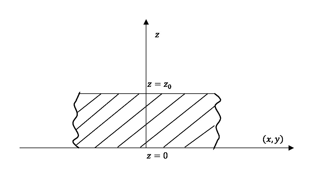
From the expression (5) our plate is confined in $0<z<z_{0}$, and in $\left(x,y\right)$ directions it extends throughout the $\left(x,y\right)$ coordinates. (FIG. 1).

The interesting property of the function $f\left(z\right)$ in (5), which makes the main motivation of this study is that it satisfies the distributional property

where a ’prime’ means $\frac{d}{dz}$. By virtue of this condition, we have $f^{{}^{\prime\prime}}\left(z\right)=0$, for $z>z_{0}$, and $f\left(z\right)$ must be of the form $f\left(z\right)=a+bz$. For $z<z_{0}$ on the other hand we have $f\left(z\right)=\cosh\left(a_{0}z\right)$, which corresponds to the inner solution. In summary, we have

where

We tune now our parameters such that $a=0$ and $b=1$. This particular choice admits a set of numbers given by

With this choice what we have achieved is that our spacetime takes the two possible cases 1. The outer plate metric, for $z>z_{0}$

2. The inner plate metric, for $0<z\leq z_{0}$

In the following sections we shall derive the Kasner connections, the energy-momentum and investigate the extrinsic curvature of the line elements (12) and (13).

In this section, we study geodesic equations of time-like particles for the line-element (1). Lagrangian of a free particle is $\mathcal{L}=\frac{1}{2}g_{\mu\nu}\dot{x}^{\mu}\dot{x}^{\nu}$, which explicitly reads

in which a dot denotes the derivative with respect to proper time, $\tau$. The metric is independent of $t$, $x$ and $y$, therefore we have three conserved quantities, energy, linear momenta in $x$ and $y$ direction,which are shown by $E$, $\alpha_{0}$ and $\beta_{0}$. From the Euler-Lagrange equations we obtain the first integrals from the equations of motion as follows

By the definition of $4-$velocity normalization for massive particle, $g_{\mu\nu}\frac{dx^{\mu}}{d\tau}\frac{dx^{\nu}}{d\tau}=1$, and replacing conserved quantities in this equation we get the geodesics equation for $z$ coordinate as follows

Note that for calculating $z\left(t\right)$ we used $\left(\frac{\overset{\cdot}{z}}{\overset{\cdot}{t}}\right)^{2}=\left(\frac{dz}{dt}\right)^{2}$. The result will be

After the second differentiation, we obtain the acceleration

Now we will solve this differential equation for the ”outside” of an infinite plate by choosing specific constraints on $k$, to study the behavior of the particle. From now on we make the choice $k\left(k-1\right)=\frac{1}{2}$,  For the ”outside” of the infinite plate, we keep the general form $f\left(z\right)=a+bz$, so that

We reexpress Eq (35) in the following form in order to derive the speed in terms of energy

where

and by imposing the initial values of particle, $\nu_{i}=$ the initial speed, $f_{i\text{ }}$, $G_{i}$, at $t=t_{i}$ we have

It is seen from (36) that for the motion perpendicular to the plate $\left(\alpha_{0}=0=\beta_{0}\right)$ we obtain

In particular, the free fall problem $\left(\nu_{i}=0\right)$, gives

as in the Newtonian fall. Near to the plate $z\thickapprox z_{0}$ the acceleration turns out to be $a=\frac{b}{2E^{2}}$. Which determines the G-force of the plate in acceleration with Newoton’s law.

For comparable momenta $\alpha_{0}$ and $\beta_{0}$, we observe that the acceleration (36) remains negative. Far away from the plate $\left(z\gg z_{0}\right)$ attraction holds also true irrespective of $\alpha_{0}$ and $\beta_{0}$. The ambiguity of the repulsive effect, however, can be removed completely by choosing $\alpha_{0}>\beta_{0}$ for $2k-1=-\sqrt{3}\left(\text{ and }\beta_{0}>\alpha_{0}\text{ for }2k-1=+\sqrt{3}\right)$, which are the admissible values for $k$ in the assumed constraint $k\left(k-1\right)=\frac{1}{2}$.

We considered the class of Kasner metrics depending on the space coordinate $z$ instead of time as a representation of a plate of thickness $z_{0}$. We have studied the possibility of falling on such a plate. In Newtonian gravity near the Earth, an object makes a free fall motion with a constant negative acceleration. In the presence of repulsive forces of general relativity metrics, we remind that these requirements of fall are not automatically satisfied. Our plate metric fails to satisfy the weak energy condition (WEC) whose violation becomes minimized for the free parameter $k\gg 1$ or, as in other physical systems in order to provide physicality of our plate metric other physical fields must be coupled. On the other hand, the plate metric is entirely regular whose Kretchmann scalar is finite everywhere. It is observed that the choice of the stress tensor $T_{zz}=0$, is effective in making everything regular. The geodesic analysis shows that for certain $k$ values falling with a constant negative acceleration holds true as in Newton’s theory. Specifically, $k=\frac{1{\mp}\sqrt{3}}{2}$, proves to be a good choice which corresponds to the Kasner exponents $p_{1}=\frac{1}{3}$, $p_{2}=\frac{1{\mp}\sqrt{3}}{3}$ and $p_{3}=\frac{1{\pm}\sqrt{3}}{3}$. The tuning of momenta along $x$ and $y$ makes also the fall but the acceleration is not a constant. Finally, we comment that a comparison of our plate geometry with the domain wall spacetime 234 suggests that the thin-wall boundary can be extended to a thick-wall in a special direction.

References

• (1) E. Kasner, ”Geometrical theorems on Einstein’s cosmological equations”, Amer. J. Math. 43, 217-21 (1921).
• (2) A. H. Taub, ”Isentropic hydrodynamics in plane symmetric spacetimes”, Phys.Rev. 103, 454-467 (1956).
• (3) J. Ipser and P. Sikivie, ”Gravitationally repulsive domain wall”, Phys.Rev. D 30, 712-719 (1984).
• (4) A. Vilenkin ”Gravitational field of vacuum domain walls and stings”, Phys. Rev. D 23, 852-857 (1981).
• (5) M. Halilsoy and M. Odeh, ”Metric for a Thick-plate of Infinite Extent”, Eastern Mediterranean.University, preprint 2006 (unpublished)
• (6) P. Jones, G. Munoz, M. Ragsdale and D. Singleton, ”The general relativistic infinite plane”, Am. J. Phys. 76, 73-78 (2008).
• (7) C. W. Misner, K.S. Thorne and J. A. Wheeler. ”Gravitation”, (Freeman, San Francisco, 1973).