Fundamental CRB-Rate Tradeoff in Multi-Antenna ISAC Systems with Information Multicasting and Multi-Target Sensing

Zixiang Ren Yunfei Peng Xianxin Song Yuan Fang Ling Qiu Liang Liu Derrick Wing Kwan Ng Jie Xu Thanks: Part of this paper has been presented at the 2022 IEEE Global Communications Conference workshop, 4-8 December 2022, Rio de Janeiro, Brazil [1]. Thanks: Z. Ren is with Key Laboratory of Wireless-Optical Communications, Chinese Academy of Sciences, School of Information Science and Technology, University of Science and Technology of China, and the Future Network of Intelligence Institute (FNii), The Chinese University of Hong Kong (Shenzhen), Shenzhen, China (e-mail: rzx66@mail.ustc.edu.cn). Thanks: Y. Peng, X. Song, Y. Fang, and J. Xu are with the School of Science and Engineering (SSE) and the FNii, The Chinese University of Hong Kong (Shenzhen), Shenzhen, China (e-mail: 117010214@link.cuhk.edu.cn, xianxinsong@link.cuhk.edu.cn, fangyuan@cuhk.edu.cn, xujie@cuhk.edu.cn). Thanks: L. Qiu is with Key Laboratory of Wireless-Optical Communications, Chinese Academy of Sciences, School of Information Science and Technology, University of Science and Technology of China (e-mail: lqiu@ustc.edu.cn). Thanks: L. Liu is with the Department of Electronic and Information Engineering, The Hong Kong Polytechnic University, Hong Kong SAR, China (e-mails: liang-eie.liu@polyu.edu.hk). Thanks: D. W. K. Ng is with the University of New South Wales, Sydney, NSW 2052, Australia (e-mail: w.k.ng@unsw.edu.au). Thanks: L. Qiu and J. Xu are the corresponding authors.

Abstract

This paper investigates the performance tradeoff for a multi-antenna integrated sensing and communication (ISAC) system with simultaneous information multicasting and multi-target sensing, in which a multi-antenna base station (BS) sends the common information messages to a set of single-antenna communication users (CUs) and estimates the parameters of multiple sensing targets based on the echo signals concurrently. We consider two target sensing scenarios without and with prior target knowledge at the BS, in which the BS is interested in estimating the complete multi-target response matrix and the target reflection coefficients/angles, respectively. First, we consider the capacity-achieving transmission and characterize the fundamental tradeoff between the achievable rate and the multi-target estimation Cramér-Rao bound (CRB) accordingly. To this end, we design the optimal transmit signal covariance matrix at the BS to minimize the estimation CRB for each of the two scenarios, subject to the minimum multicast rate requirement and the maximum transmit power constraint. It is shown that the optimal covariance matrix consists of two parts for ISAC and dedicated sensing, respectively. Next, we consider the transmit beamforming designs, in which the BS sends one information beam together with multiple a-priori known dedicated sensing beams for effective ISAC and each CU can cancel the interference caused by the sensing signals. By exploiting the successive convex approximation (SCA) technique, we develop efficient algorithms to obtain the joint information and sensing beamforming solutions to the resultant rate-constrained CRB minimization problems. Finally, we provide numerical results to validate the CRB-rate (C-R) tradeoff achieved by our proposed designs, as compared to two benchmark schemes, namely the isotropic transmission and the joint beamforming without sensing interference cancellation. It is shown that the proposed optimal transmit covariance solution achieves much better C-R performance than the benchmark schemes and the proposed joint beamforming with sensing interference cancellation performs close to the optimal transmit covariance solution when the number of CUs is small. We also conduct simulations to show the practical estimation performance achieved by our proposed designs, by considering randomly generated information signals and practical estimators.

Index Terms:

Integrated sensing and communications (ISAC), multicast channel, multi-target sensing, Cramér-Rao bound (CRB), transmit beamforming, optimization.

I Introduction

Future beyond fifth-generation (B5G) and sixth-generation (6G) wireless networks are envisioned to support abundant intelligent applications such as the metaverse, auto-driving, smart homes, and smart cities, which demand ultra-high-capacity, ultra-low-latency, and ultra-high reliable communications, as well as high-accuracy and high-resolution sensing. Towards this end, integrated sensing and communication (ISAC) has emerged as a promising technology for realizing B5G/6G, which enables the dual use of radio signals and wireless network infrastructures for providing both sensing and communication services simultaneously [2]. By seamlessly coordinating and integrating sensing and communications [3], ISAC is expected to significantly enhance both communication and sensing performances, while improving the spectrum utilization efficiency and the cost efficiency. As such, ISAC has recently attracted tremendous research interests in both academia and industry [4], motivating extensive studies on ISAC from different research perspectives such as unified ISAC waveforms [2], multi-antenna ISAC [3], networked ISAC [5, 6], wideband ISAC [2], and intelligent reflecting surface (IRS)-enabled ISAC [7, 8].

Among various enabling techniques, multiple-input multiple-output (MIMO) has been recognized as an important solution to enhance the performance of wireless networks, by equipping multiple antennas at the wireless transceivers, e.g., base stations (BSs). In particular, MIMO can provide potential spatial multiplexing and diversity gains to increase the communication rate and reliability [9], while offering spatial and waveform diversity gains to enhance the sensing accuracy and resolution [10, 11]. Indeed, how to optimize the transmit waveform and beamforming design based on proper sensing and communication performance metrics is a key technical challenge to be tackled for multi-antenna ISAC. On the one hand, for communication, the signal-to-interference-plus-noise ratio (SINR) and data rate are widely adopted as performance measures. On the other hand, for sensing, various performance measures may apply depending on the specific sensing tasks. For instance, when the sensing estimation tasks for target detection and tracking [12] are considered, the estimation mutual information [13], radar sensing SINR [14], transmit beampattern [15], and Cramér-Rao bound (CRB) [16] are widely applied, among which the beampattern and CRB-based designs are most promising. The basic idea of beampattern-based design is to match the transmitted beampattern with a pre-defined sensing beampattern such that the transmit signal beams are focused towards the desired target directions and those leaked to the other undesired directions are suppressed as possible. There have been extensive existing works considering the waveform/beamforming design based on the transmit beampattern. For example, the authors in [17, 15, 18] studied the downlink ISAC over broadcast channels by considering different setups, in which the transmit beamforming was optimized to properly balance the tradeoff between the transmit beampattern for sensing and the received SINR for communication. These designs were then extended to the case of downlink non-orthogonal multiple access (NOMA) in [19]. However, aiming to mimic the transmit beampattern may not be able to capture the quality of sensing directly and thus may lead to sacrificed sensing performances.

In contrast to the transmit beampattern, the CRB has been recognized as a practically relevant and analytically tractable metric to directly measure the sensing performance limits for estimating target parameters. In general, the CRB provides the lower bound of variance for any unbiased estimators, which can be derived by exploiting the Fisher information matrix to measure the amount of information that the data provides about the parameter of interest [12, 16, 20, 21]. As a result, directly optimizing the CRB is a viable new approach that is suitable for designing ISAC systems, which not only facilitates the characterization of the fundamental CRB-rate (C-R) performance tradeoff, but also leads to potentially enhanced parameter estimation performances. For instance, the authors in [16] studied the multiuser ISAC over a broadcast channel with one single-target, in which the transmit beamforming was optimized to minimize the estimation CRB, subject to the individual SINR (or equivalently rate) constraints at multiple communication users (CUs). Furthermore, [20] and [21] investigated the C-R tradeoff in a point-to-point MIMO ISAC system with one CU and one target. In particular, the authors in [21] optimized the transmit covariance to characterize the complete Pareto boundary of the C-R region for the MIMO ISAC system in two specific scenarios with point and extended target models, respectively, by considering the radar coherent processing interval to be sufficiently long. As for [20], the authors revealed the C-R tradeoff for a more general case with finite radar coherent processing intervals. In addition, [22] investigated the C-R tradeoff for ISAC in multi-antenna broadcast channels, in which the emerging rate-splitting multiple access (RSMA) technique was exploited to further improve the ISAC performance.

With recent advancements in webcast and content broadcasting applications, it has become crucial for future B5G/6G wireless networks to effectively support simultaneous data transmission to multiple users through multicast channels [23, 24]. Additionally, the ability to conduct multi-target sensing and tracking plays a vital role in various multicast applications, such as surveillance, object detection, and autonomous vehicles [4]. Consequently, supporting efficient ISAC over multi-antenna systems during such information multicasting has become an increasingly important problem. This problem, however, is particularly challenging. This is due to the fact that the transmission principle for multicast channels significantly differs from that for broadcast channels, thus rendering the prior ISAC designs [16, 22, 21, 20] over broadcast channels not applicable. To illustrate this, we consider a multiple-input single-output (MISO) multicast channel as an example. First, it has been demonstrated in [23] that achieving the MISO multicast capacity typically requires a high-rank transmit covariance matrix for transmitting common messages. This stands in contrast to the MISO broadcast channel, where the capacity is achievable by employing a rank-one covariance matrix for each user’s individual message along with dirty paper coding [25]. Next, it has been shown in [24] that in MISO multicast channels, the transmit beamforming optimization problem for minimizing the transmit power while ensuring individual users’ signal-to-noise ratio (SNR) requirements is an NP-hard problem. This is distinct from the MISO broadcast channels, in which the transmit beamforming design for SINR-constrained power minimization has been proven to be a convex problem [26, 27]. Due to such significant differences, new design approaches and principles are needed for ISAC over multicast channels, thus motivating our investigation in this work.

This paper investigates the multi-antenna ISAC over a multicast channel with multi-target sensing, in which a multi-antenna BS sends common messages to a set of single-antenna CUs and simultaneously exploits the received echo signals to estimate the parameters of multiple sensing targets. In particular, we consider two scenarios for multi-target sensing without and with prior target knowledge at the BS, namely Scenario I and Scenario II, respectively. In practice, Scenarios I and II may correspond to the target detection and target tracking stages for multi-target sensing, respectively.¹¹ 1 In general, the BS often lacks prior knowledge of the targets before transmission. Therefore, an initial target detection stage is required, in which the ISAC signal transmission is designed to estimate the complete multi-target response matrix for extracting multi-target parameters. With the obtained target parameters at hand, a subsequent target tracking stage is implemented, in which the ISAC signal transmission is designed by leveraging such a piece of prior information to facilitate the tracking of these targets or the estimation of their reflection coefficients and angles. The main results of our work are summarized as follows.

•

First, we consider the capacity-achieving transmission, based on which we characterize the fundamental performance tradeoff between the estimation CRB for multi-target sensing versus the channel capacity for information multicasting in the two scenarios, which generalizes the target sensing study compared with [1]. To this end, we minimize the corresponding estimation CRB for each scenario, by optimizing the transmit covariance matrix at the BS, subject to the minimum multicast rate constraint and the maximum transmit power constraint. We obtain the globally optimal solutions to the two rate-constrained CRB minimization problems by applying advanced convex optimization techniques. For both scenarios, the optimal transmit covariance is shown to consist of two signal parts for ISAC and dedicated sensing, respectively.
•

Next, to facilitate the implementation, we present new joint information and sensing beamforming designs for efficient ISAC. In such designs, the BS sends one common information beam together with multiple dedicated a-priori known sensing beams such that each CU is capable of canceling the interference caused by these sensing beams. For each of the two scenarios, we develop a computationally efficient algorithm by adopting the successive convex approximation (SCA) technique to obtain a high-quality joint beamforming solution for minimizing the multi-target estimation CRB while ensuring the minimum multicast rate requirement.
•

Finally, we provide numerical results to validate the C-R tradeoff performance achieved by our proposed designs, as compared to two benchmark schemes, namely the isotropic transmission and the joint beamforming without sensing interference cancellation. It is shown that for each scenario, the proposed designs significantly outperform the two benchmark schemes and the proposed joint beamforming with sensing interference cancellation achieves performance close to the upper bound achieved by the optimal transmit covariance when the number of CUs is small. We also perform simulations to assess the estimation performance using randomly generated information signals and practical estimators. The results clearly demonstrate that our CRB minimization designs significantly reduce the root mean squared error (RMSE) of estimation compared to conventional beampattern-based designs. This highlights the superior performance and feasibility of our proposed designs in the practical ISAC implementation and provides more comprehensive performance comparison than [1].

The remainder of this paper is organized as follows. Section II introduces the multicast multi-target ISAC system model and formulates the multicast-rate-constrained CRB minimization problems for Scenarios I and II when the BS does not and does have the prior multi-target knowledge, respectively. Sections III and IV develop the optimal solutions to the formulated multicast-rate-constrained CRB minimization problems for Scenarios I and II, respectively. Section V proposes joint information and sensing beamforming designs with sensing interference pre-cancellation at the CUs. Section VI provides numerical results. Finally, Section VII concludes this paper.

Notations: Vectors and matrices are denoted by bold lower- and upper-case letters, respectively. $\mathbb{C}^{N\times M}$ denotes the space of $N\times M$ complex matrices. $\boldsymbol{I}$ and $\boldsymbol{0}$ represent an identity matrix and an all-zero matrix with appropriate dimensions, respectively. For a square matrix $\boldsymbol{A}$ , $\textrm{tr}(\boldsymbol{A})$ denotes its trace and $\boldsymbol{A}\succeq\boldsymbol{0}$ means that $\boldsymbol{A}$ is positive semi-definite. For a complex arbitrary-size matrix $\boldsymbol{B}$ , $\boldsymbol{B}[i,j]$ , $\textrm{rank}(\boldsymbol{B})$ , $\boldsymbol{B}^{T}$ , $\boldsymbol{B}^{H}$ , and $\boldsymbol{B}^{c}$ denote its $(i,j)$ -th element, rank, transpose, conjugate transpose, and complex conjugate, respectively, and $\mathrm{vec}(\boldsymbol{B})$ denotes the vectorization of $\boldsymbol{B}$ . For a vector $\boldsymbol{a}$ , $\boldsymbol{a}[i]$ denotes its $i$ -th element. $\mathbb{E}(\cdot)$ denotes the statistical expectation. $\|\cdot\|$ denotes the Euclidean norm of a vector. $|\cdot|$ , $\mathrm{Re}(\cdot)$ , and $\mathrm{Im}(\cdot)$ denote the absolute value, the real component, and the imaginary component of a complex entry. $\mathcal{CN}(\boldsymbol{x},\boldsymbol{Y})$ denotes a circularly symmetric complex Gaussian (CSCG) random vector with mean vector $\boldsymbol{x}$ and covariance matrix $\boldsymbol{Y}$ . $\boldsymbol{A}\otimes\boldsymbol{B}$ and $\boldsymbol{A}\odot\boldsymbol{B}$ represent the Kronecker product and Hadamard product of two matrices $\boldsymbol{A}$ and $\boldsymbol{B}$ , respectively.

II System Model and Problem Formulation

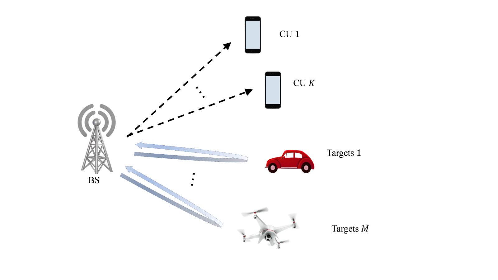
Refer to caption — Fig. 1: Illustration of the multi-antenna ISAC system for simultaneous information multicasting and multi-target sensing.

As shown in Fig. 1, we consider a multi-antenna ISAC system for information multicasting and multi-target sensing, which consists of a multi-antenna BS equipped with $N_{t}$ transmit antennas and $N_{r}$ receive antennas, $K$ single-antenna CUs, and $M$ sensing targets. Let $\mathcal{K}\overset{\bigtriangleup}{=}\{1,2,\ldots,K\}$ denote the set of CUs and $\mathcal{M}\overset{\bigtriangleup}{=}\{1,2,\ldots,M\}$ denote that of sensing targets. The BS sends common information signals to all the CUs and exploits the received echo signals to sense the $M$ targets simultaneously. In particular, we focus on the ISAC period consisting of $L$ symbols. In this paper, we focus on a quasi-static environment, where the communication and sensing channels are assumed to remain invariant during the ISAC period, similar to [16, 28]. Let $\boldsymbol{x}(n)\in\mathbb{C}^{N_{t}\times 1}$ denote the transmitted ISAC signal by the BS in symbol $n\in\mathcal{L}\triangleq\{1,2,\ldots,L\}$ . For achieving the multicast capacity, we consider that the transmitted signal $\boldsymbol{x}(n)$ is a CSCG random vector with zero mean and covariance $\mathbb{E}[\boldsymbol{x}(n)\boldsymbol{x}^{H}(n)]=\boldsymbol{S}_{x}\succeq\boldsymbol{0}$ , i.e., $\boldsymbol{x}(n)\sim\mathcal{CN}(\boldsymbol{0},\boldsymbol{S}_{x}),\forall n$ . Supposing that the BS is subject to a maximum transmit power budget $P$ , we have

\mathrm{tr}(\boldsymbol{S}_{x})\leq P.

(1)

II-A Multicasting Communication Model

First, we consider the multicast channel for communication. Let $\boldsymbol{h}_{k}\in\mathbb{C}^{N_{t}\times 1}$ denote the channel vector from the BS to CU $k\in\mathcal{K}$ . The received signal at the receiver of CU $k\in\mathcal{K}$ is given by [23]

y_{k}(n)=\boldsymbol{h}_{k}^{H}\boldsymbol{x}(n)+z_{k}(n),\forall n\in\mathcal{L},

(2)

where $z_{k}(n)$ denotes the noise at the receiver of CU $k$ that is a CSCG random variable with zero mean and variance $\sigma^{2}$ , i.e., $z_{k}(n)\sim\mathcal{CN}(0,\sigma^{2}),\forall k\in\mathcal{K}$ . Based on the received signal in (2), the received SNR at CU $k\in\mathcal{K}$ is²² 2 Since all the receivers require the same common message from one single BS, there is no multi-user interference. On the other hand, the co-channel interference from other radio transmitters in the environment can be included in $z_{k}(n)$ such that $\sigma^{2}$ captures the impacts caused by background interference.

\gamma_{k}(\boldsymbol{S}_{x})=\mathbb{E}\bigg(\frac{\big|\boldsymbol{h}_{k}^{H}\boldsymbol{x}(n)\big|^{2}}{\big|z_{k}(n)\big|^{2}}\bigg)=\frac{\boldsymbol{h}_{k}^{H}\boldsymbol{S}_{x}\boldsymbol{h}_{k}}{\sigma^{2}}.

(3)

Accordingly, the achievable rate of the multicast channel with a given transmit covariance $\boldsymbol{S}_{x}$ is given by [23, 24]

R(\boldsymbol{S}_{x})=\underset{k\in\mathcal{K}}{\min}\Big\{\log_{2}\Big(1+\frac{\boldsymbol{h}_{k}^{H}\boldsymbol{S}_{x}\boldsymbol{h}_{k}}{\sigma^{2}}\Big)\Big\}.

(4)

As a result, the capacity of the multicast channel is defined as the maximum achievable rate, given by [23, 24]

C_{0}=\underset{\boldsymbol{S}_{x}\succeq\boldsymbol{0},\mathrm{tr}(\boldsymbol{S}_{x})\leq P}{\max}R(\boldsymbol{S}_{x}).

(5)

II-B Multi-target Sensing Model

Next, we consider the multi-target radar sensing, in which the BS adopts its $N_{r}$ receive antennas for receiving the echo signals to estimate the parameters of the $M$ sensing targets. Suppose that these $M$ targets are located in the same range bin of the far-field region of the BS. In this case, the received target echo signals at the BS in symbol $n\in\mathcal{L}$ is expressed as³³ 3 Similar as in prior works on ISAC and radar sensing [16, 21], we ignore the self-interference due to the signal transmission in (5), as the sensing receiver can handle such an issue properly [29]. This is different from the communication receivers, for which the self-interference might be a severe issue. Furthermore, similar to prior works on MIMO radar sensing [11, 28] and MIMO ISAC [2], we consider the estimation of target angles and complex coefficients based on the echo signals in (6), in which the Doppler effects are omitted.

\boldsymbol{y}(n)=\sum_{m=1}^{M}\beta_{m}\boldsymbol{a}_{r}^{c}(\theta_{m})\boldsymbol{a}_{t}^{H}(\theta_{m})\boldsymbol{x}(n)+\boldsymbol{\boldsymbol{z}}(n),

(6)

where $\beta_{m}\in\mathbb{C}$ denotes the complex coefficient of target $m\in\mathcal{M}$ whose amplitude captures the round-trip path loss and is proportional to its radar cross section (RCS) [30, 28], $\theta_{m}$ denotes the angle of departure (AoD)/angle of arrival (AoA) of target $m\in\mathcal{M}$ , $\boldsymbol{a}_{r}(\theta)\in\mathbb{C}^{N_{r}\times 1}$ and $\boldsymbol{a}_{t}(\theta)\in\mathbb{C}^{N_{t}\times 1}$ denote the receive and transmit steering vectors with angle $\theta$ , respectively, and $\boldsymbol{z}(n)\sim\mathcal{CN}(\boldsymbol{0},\sigma_{r}^{2}\boldsymbol{I})$ is the noise at the BS receiver with $\sigma_{r}^{2}$ being the noise power at each receive antenna. Let $\boldsymbol{X}=[\boldsymbol{x}(1),\dots,\boldsymbol{x}(L)]$ denote the transmitted signal over the $L$ symbols. By assuming that $L$ is sufficiently large, the sample covariance matrix of $\boldsymbol{X}$ can be approximated as the statistical covariance matrix⁴⁴ 4 We will show that the approximation is sufficiently accurate for practical values of $L$ (e.g., $L\geq 64$ ) in the numerical results in Section VI. $\boldsymbol{S}_{x}$ , i.e.,

\frac{1}{L}\boldsymbol{X}\boldsymbol{X}^{H}\approx\boldsymbol{S}_{x}.

(7)

To facilitate the derivation of the CRB matrix for estimating the parameters of targets, we rewrite (6) as

\boldsymbol{Y}=\boldsymbol{A}_{r}^{c}\boldsymbol{B}\boldsymbol{A}_{t}^{H}\boldsymbol{X}+\boldsymbol{Z},

(8)

where $\boldsymbol{Y}=[\boldsymbol{y}(1),...,\boldsymbol{y}(L)]$ , $\boldsymbol{Z}=[\boldsymbol{z}(1),...,\boldsymbol{z}(L)]$ , $\boldsymbol{A}_{r}=[\boldsymbol{a}_{r}(\theta_{1})$ , $\boldsymbol{a}_{r}(\theta_{2}),\dots,\boldsymbol{a}_{r}(\theta_{M})]$ , $\boldsymbol{A}_{t}=[\boldsymbol{a}_{t}(\theta_{1}),\boldsymbol{a}_{t}(\theta_{2}),\dots,\boldsymbol{a}_{t}(\theta_{M})]$ , $\boldsymbol{\theta}=[\theta_{1},\theta_{2},\dots,\theta_{M}]^{T},\boldsymbol{\beta}=[\beta_{1},\beta_{2},\dots,\beta_{M}]^{T}$ , and $\boldsymbol{B}=\mathrm{diag}(\boldsymbol{\beta})$ . Let $\boldsymbol{G}=\boldsymbol{A}_{r}^{c}\boldsymbol{B}\boldsymbol{A}_{t}^{H}$ denote the multi-target response matrix. Accordingly, we vectorize (8) as

\tilde{\boldsymbol{y}}=(\boldsymbol{X}^{T}\otimes\boldsymbol{I}_{N_{r}})\tilde{\boldsymbol{g}}+\tilde{\boldsymbol{z}},

(9)

where $\tilde{\boldsymbol{y}}=\mathrm{vec}(\boldsymbol{Y})\in\mathbb{C}^{N_{r}L\times 1}$ , $\tilde{\boldsymbol{g}}=\mathrm{vec}(\boldsymbol{G})\in\mathbb{C}^{N_{r}N_{t}\times 1},$ and $\tilde{\boldsymbol{z}}=\mathrm{vec}(\boldsymbol{Z})\in\mathbb{C}^{N_{r}L\times 1}$ . It follows from (9) that the received signal vector $\tilde{\boldsymbol{r}}$ is a CSCG random vector with mean $(\boldsymbol{X}^{T}\otimes\boldsymbol{I})\tilde{\boldsymbol{g}}$ and covariance $\sigma_{r}^{2}\boldsymbol{I}$ , i.e., $\tilde{\boldsymbol{y}}\sim\mathcal{CN}\big((\boldsymbol{X}^{T}\otimes\boldsymbol{I})\tilde{\boldsymbol{g}},\sigma_{r}^{2}\boldsymbol{I}\big)$ .

In particular, we consider two different sensing scenarios, namely Scenario I and Scenario II, in which the BS does not and does have a-prior knowledge about the multiple targets such that the BS aims to estimate the complete multi-target response matrix $\boldsymbol{G}=\boldsymbol{A}_{r}^{c}\boldsymbol{B}\boldsymbol{A}_{t}^{H}$ and the targets’ coefficients/angles (i.e., $\{\beta_{m}\}_{m=1}^{M}$ and $\{\theta_{m}\}_{m=1}^{M}$ ), respectively. In practice, Scenario I may correspond to the target detection phase, in which the BS tries to identify the number of targets and obtain their parameters based on matrix $\boldsymbol{G}$ via spatial spectrum algorithms such as multiple signal classification (MUSIC). On the other hand, Scenario II may correspond to the target tracking phases, in which the BS needs to track the $M$ targets by estimating their coefficients/angles, with their initial parameters known in advance [31, 32], respectively.

II-B1 CRB for Estimating $\boldsymbol{G}$ in Scenario I

First, we consider Scenario I, in which the BS lacks prior knowledge of the targets in the initial target detection stage [33, 2]. In this scenario, the BS is interested in estimating the complete multi-target response matrix $\boldsymbol{G}=\boldsymbol{A}_{r}^{c}\boldsymbol{B}\boldsymbol{A}_{t}^{H}$ based on the received signal $\boldsymbol{Y}$ in (8), or equivalently estimating $\tilde{\boldsymbol{g}}$ based on $\tilde{\boldsymbol{r}}$ in (9). After obtaining the estimate of $\boldsymbol{G}$ , the BS can further implement spatial spectrum algorithms such as MUSIC[34] to further extract the angle information of these targets. In this scenario, the BS needs to estimate $N_{r}N_{t}$ complex parameters in $\tilde{\boldsymbol{g}}$ or $\boldsymbol{G}$ . Based on the complex linear model in (9), it has been established in [35] that the CRB matrix for estimating $\tilde{\boldsymbol{g}}$ is

\displaystyle\boldsymbol{C}_{1}\negthickspace=

\displaystyle\big((\boldsymbol{X}^{T}\otimes\boldsymbol{I}_{N_{r}})^{H}(\sigma_{r}^{2}\boldsymbol{I})^{-1}(\boldsymbol{X}^{T}\otimes\boldsymbol{I}_{N_{r}})\big)^{-1}\negthickspace\negthickspace=\sigma_{r}^{2}\big(\boldsymbol{X}^{c}\boldsymbol{X}^{T}\otimes\boldsymbol{I}_{N_{r}}\big)^{-1}\negthickspace\overset{(\mathrm{a})}{=}\frac{\sigma_{r}^{2}}{L}\big(\boldsymbol{S}_{x}^{T}\otimes\boldsymbol{I}_{N_{r}}\big)^{-1},

(10)

where (a) follows from the approximation in (7). For facilitating the sensing performance optimization, scalar functions of the CRB matrix are normally adopted as the performance metrics, some examples include trace, determinant, and minimum eigenvalue (10). In this paper, we adopt its trace as the scalar performance metric, i.e.

\mathrm{CRB}_{1}(\boldsymbol{S}_{x})=\frac{N_{r}\sigma_{r}^{2}}{L}\mathrm{tr}(\boldsymbol{S}_{x}^{-1}).

(11)

Intuitively, $\mathrm{CRB}_{1}(\boldsymbol{S}_{x})$ corresponds to the sum of the CRBs for estimating the elements in $\boldsymbol{G}$ .

II-B2 CRB for Estimating $\boldsymbol{\theta}$ and $\boldsymbol{\beta}$ in Scenario II

Next, we consider Scenario II, in which the BS has a priori knowledge of the multiple targets (e.g., from the target detection stage), and thus is interested in estimating the target coefficients $\boldsymbol{\beta}$ and angles $\boldsymbol{\theta}$ as unknown parameters. This may correspond to the target tracking stage in practice [33, 2]. Let $\boldsymbol{\beta}_{R}=[\mathrm{Re}(\beta_{1}),\mathrm{Re(}\beta_{2}),\dots,\mathrm{Re(}\beta_{M})]^{T}$ and $\boldsymbol{\beta}_{I}=[\mathrm{Im}(\beta_{1}),\mathrm{Im(}\beta_{2}),\dots,\mathrm{Im(}\beta_{M})]^{T}$ denote the real and imaginary parts of $\boldsymbol{\beta}$ . Accordingly, we have a total of $3M$ real parameters to be estimated, given by $\boldsymbol{\xi}=[\boldsymbol{\theta}^{T},\boldsymbol{\text{$\beta$}}_{R}^{T},\boldsymbol{\beta}_{I}^{T}]$ ^T. To facilitate the CRB derivation, we have the following lemma [35].

Lemma 1.

[35] Consider the estimation of real-valued parameters $\boldsymbol{\varsigma}\in\mathbb{R}^{T\times 1}$ based on the CSCG data vector $\tilde{\boldsymbol{v}}\in\mathbb{C}^{N\times 1}$ , i.e., $\tilde{\boldsymbol{v}}\sim\mathcal{CN}(\tilde{\boldsymbol{\mu}}(\boldsymbol{\varsigma}),\boldsymbol{C}_{\tilde{\boldsymbol{v}}})$ , where the covariance $\boldsymbol{C}_{\tilde{\boldsymbol{v}}}$ is independent from parameters $\boldsymbol{\varsigma}$ . The Fisher information matrix (FIM) for estimating $\boldsymbol{\varsigma}$ is given by $\boldsymbol{F}_{\boldsymbol{\varsigma}}$ , with

\boldsymbol{F}_{\boldsymbol{\varsigma}}[i,j]=2\mathrm{Re}\Big(\frac{\partial\tilde{\boldsymbol{\mu}}^{H}(\boldsymbol{\varsigma})}{\partial\boldsymbol{\varsigma}[i]}\boldsymbol{C}_{\tilde{\boldsymbol{v}}}^{-1}\frac{\partial\tilde{\boldsymbol{\mu}}(\boldsymbol{\varsigma})}{\partial\boldsymbol{\varsigma}[j]}\Big),\forall i,j\in\{1,\ldots,T\},

(12)

where $\frac{\partial}{\partial}(\cdot)$ denotes the partial derivative operator.

Notice that based on (9), we have $\tilde{\boldsymbol{y}}\sim\mathcal{CN}\big(\mathrm{vec}(\boldsymbol{A}_{r}^{c}\boldsymbol{B}\boldsymbol{A}_{t}^{H}\boldsymbol{X}),\sigma_{r}^{2}\boldsymbol{I}\big)$ . Let $\boldsymbol{F}_{\boldsymbol{\xi}}\in\mathbb{R}^{3M\times 3M}$ denote the FIM for estimating $\boldsymbol{\xi}$ . Based on Lemma 1, the element in the $i$ -th row and $j$ -th column of $\boldsymbol{F}_{\boldsymbol{\xi}}$ , $\forall i,j\in\{1,\ldots,3M\}$ , is given by

\displaystyle\boldsymbol{F}_{\boldsymbol{\xi}}[i,j]

\displaystyle=

\displaystyle\frac{2}{\sigma_{r}^{2}}\mathrm{Re}\Big(\frac{\partial\mathrm{vec}(\boldsymbol{A}_{r}^{c}\boldsymbol{B}\boldsymbol{A}_{t}^{H}\boldsymbol{X})^{H}}{\partial\boldsymbol{\boldsymbol{\xi}}[i]}\cdot\frac{\partial\mathrm{vec}(\boldsymbol{A}_{r}^{c}\boldsymbol{B}\boldsymbol{A}_{t}^{H}\boldsymbol{X})}{\partial\boldsymbol{\boldsymbol{\xi}}[j]}\Big),

(13)

where $\dot{\boldsymbol{A}_{r}}=[\frac{\partial\boldsymbol{a}_{r}(\theta_{1})}{\partial\theta_{1}},\frac{\partial\boldsymbol{a}_{r}(\theta_{2})}{\partial\theta_{2}},\cdots,\frac{\partial\boldsymbol{a}_{r}(\theta_{M})}{\partial\theta_{M}}],$ and $\dot{\boldsymbol{A}_{t}}=[\frac{\partial\boldsymbol{a}_{t}(\theta_{1})}{\partial\theta_{1}},\frac{\partial\boldsymbol{a}_{t}(\theta_{2})}{\partial\theta_{2}},\cdots,\frac{\partial\boldsymbol{a}_{t}(\theta_{M})}{\partial\theta_{M}}].$ Following the similar derivation procedures in [28], we have the FIM in a block matrix form:

\boldsymbol{F}_{\boldsymbol{\xi}}=\frac{2}{\sigma_{r}^{2}}\left[\begin{array}[]{ccc}\mathrm{Re}(\boldsymbol{F}_{11})&\mathrm{Re}(\boldsymbol{F}_{12})&-\mathrm{Im}(\boldsymbol{F}_{12})\\ \mathrm{Re}(\boldsymbol{F}_{12})^{T}&\mathrm{Re}(\boldsymbol{F}_{22})&-\mathrm{Im}(\boldsymbol{F}_{22})\\ -\mathrm{Im}(\boldsymbol{F}_{12})^{T}&-\mathrm{Im}(\boldsymbol{F}_{22})^{T}&\mathrm{Re}(\boldsymbol{F}_{22})\end{array}\right],

(14)

where

$\displaystyle\boldsymbol{F}_{11}$	$\displaystyle=$	$\displaystyle L(\dot{\boldsymbol{A}_{r}}^{T}\dot{\boldsymbol{A}_{r}}^{c})\odot(\boldsymbol{B}^{c}\boldsymbol{A}_{t}^{T}\boldsymbol{S}_{x}^{T}\boldsymbol{A}_{t}^{c}\boldsymbol{B}^{T})+L(\dot{\boldsymbol{A}_{r}}^{T}\boldsymbol{A}_{r}^{c})\odot(\boldsymbol{B}^{c}\boldsymbol{A}_{t}^{T}\boldsymbol{S}_{x}^{T}\dot{\boldsymbol{A}_{t}}^{c}\boldsymbol{B}^{T})$	(15)
		$\displaystyle+L(\boldsymbol{A}_{r}^{T}\dot{\boldsymbol{A}_{r}}^{c})\odot(\boldsymbol{B}^{c}\dot{\boldsymbol{A}_{t}}^{T}\boldsymbol{S}_{x}^{T}\boldsymbol{A}_{t}^{c}\boldsymbol{B}^{T})+L(\boldsymbol{A}_{r}^{T}\boldsymbol{A}_{r}^{c})\odot(\boldsymbol{B}^{c}\dot{\boldsymbol{A}_{t}}^{T}\boldsymbol{S}_{x}^{T}\dot{\boldsymbol{A}_{t}}^{c}\boldsymbol{B}^{T}),$	(15)
$\displaystyle\boldsymbol{F}_{12}$	$\displaystyle=$	$\displaystyle L(\dot{\boldsymbol{A}_{r}}^{T}\boldsymbol{A}_{r}^{c})\odot(\boldsymbol{B}^{c}\boldsymbol{A}_{t}^{T}\boldsymbol{S}_{x}^{T}\boldsymbol{A}_{t}^{c})+L(\boldsymbol{A}_{r}^{T}\boldsymbol{A}_{r}^{c})\odot(\boldsymbol{B}^{c}\dot{\boldsymbol{A}_{t}}^{T}\boldsymbol{S}_{x}^{T}\boldsymbol{A}_{t}^{c}),$	(16)
$\displaystyle\boldsymbol{F}_{22}$	$\displaystyle=$	$\displaystyle L(\boldsymbol{A}_{r}^{T}\boldsymbol{A}_{r}^{c})\odot(\boldsymbol{A}_{t}^{T}\boldsymbol{S}_{x}^{T}\boldsymbol{A}_{t}^{c}).$	(17)

Then, the corresponding CRB matrix for estimating $\boldsymbol{\xi}$ is

\boldsymbol{C}_{2}=\boldsymbol{F}_{\boldsymbol{\xi}}^{-1}.

(18)

Similar as in (10), we adopt the trace of the CRB matrix $\boldsymbol{C}_{2}$ as the scalar performance metric for estimating $\boldsymbol{\xi}$ , i.e.,

\mathrm{CRB}_{2}(\boldsymbol{S}_{x})=\mathrm{tr}(\boldsymbol{C}_{2})=\mathrm{tr}(\boldsymbol{F}_{\boldsymbol{\xi}}^{-1}).

(19)

II-C Problem Formulation

We are interested in revealing the fundamental C-R performance tradeoff limits of the multicast multi-target ISAC system for both Scenarios I and II. Notice that in our considered setup, the transmit multi-beam signals $\boldsymbol{X}$ are reused for both sensing and communications. This ensures the optimal performance, as adopting separate communication and sensing signal beams would lead to the degradation in both communication and sensing performances, due to the potential mutual interference between communication and sensing signals. Let $\mathcal{C}_{1}$ and $\mathcal{C}_{2}$ denote the achievable C-R regions of the ISAC system in Scenario I and II, respectively, which are defined as

\displaystyle\mathcal{C}_{i}\overset{\triangle}{=}\underset{\boldsymbol{S}_{x}\succeq\boldsymbol{0}}{\bigcup}\big\{(\hat{R},\hat{\Psi})|\hat{R}\leq R(\boldsymbol{S}_{x}),

\displaystyle\hat{\Psi}\geq\mathrm{CRB}_{i}(\boldsymbol{S}_{x}),\mathrm{tr}(\boldsymbol{S}_{x})\leq P\big\},i\in\{1,2\}.

(20)

Our objective is to characterize the Pareto boundary of each region $\mathcal{C}_{i},i\in\{1,2\}$ , at each point of which we cannot improve one criteria without sacrificing the other [21, 20]. Note that the multicast rate $R(\boldsymbol{S}_{x})$ in (4), $\mathrm{CRB}_{1}(\boldsymbol{S}_{x})$ in (11), and $\mathrm{CRB}_{2}(\boldsymbol{S}_{x})$ in (18) are both convex with respect to (w.r.t.) $\boldsymbol{S}_{x}$ . Therefore, the C-R regions $\mathcal{C}_{i},i\in\{1,2\}$ , are both convex sets. As a result, we can characterize the whole Pareto boundary by finding each boundary point via minimizing the CRB subject to varying multicast rate thresholds [21, 20, 36].

In particular, we optimize the transmit covariance matrix $\boldsymbol{S}_{x}$ to minimize the estimation CRB for multi-target estimation while ensuring a minimum multicast communication rate $\bar{R}$ , subject to a maximum transmit power constraint in (1). First, consider Scenario I, for which the multicast-rate-constrained CRB minimization problem is formulated as

$\displaystyle(\mathrm{P1}):$	$\displaystyle\underset{\boldsymbol{S}_{x}\succeq\boldsymbol{0}}{\min}$	$\displaystyle\frac{N_{r}\sigma_{r}^{2}}{L}\mathrm{tr}(\boldsymbol{S}_{x}^{-1})$	(21)
	$\displaystyle\mathrm{s.t.}$	$\displaystyle\underset{k\in\mathcal{K}}{\min}\Big\{\log_{2}\Big(1+\frac{\boldsymbol{h}_{k}^{H}\boldsymbol{S}_{x}\boldsymbol{h}_{k}}{\sigma^{2}}\Big)\Big\}\geq\bar{R},$
		$\displaystyle\mathrm{tr}(\boldsymbol{S}_{x})\leq P.$

By introducing $\Gamma=\sigma^{2}(2^{\bar{R}}-1)$ , problem (P1) is equivalently reformulated as


$\displaystyle(\mathrm{P1.1}):$	$\displaystyle\underset{\boldsymbol{S}_{x}\succeq\boldsymbol{0}}{\min}$	$\displaystyle\mathrm{tr}(\boldsymbol{S}_{x}^{-1})$	(22a)
	$\displaystyle\mathrm{s.t.}$	$\displaystyle\boldsymbol{h}_{k}^{H}\boldsymbol{S}_{x}\boldsymbol{h}_{k}\geq\Gamma,\forall k\in\mathcal{K},$	(22a)
		$\displaystyle\mathrm{tr}(\boldsymbol{S}_{x})\leq P.$	(22b)

In problem (P1.1), the objective is a trace inverse function that is strictly convex w.r.t. $\boldsymbol{S}_{x}$ [37], and the constraints in (22a) and (22b) are both affine. As a result, problem (P1.1) is a convex optimization problem. In Section III, we will obtain its globally optimal solution in a semi-closed form by applying the Lagrange duality method [36].

Next, we consider Scenario II, for which the multicast-rate-constrained CRB minimization problem is formulated as

$\displaystyle(\mathrm{P2}):$	$\displaystyle\underset{\boldsymbol{S}_{x}\succeq\boldsymbol{0}}{\min}$	$\displaystyle\mathrm{CRB}_{2}(\boldsymbol{S}_{x})$	(23)
	$\displaystyle\mathrm{s.t.}$	$\displaystyle\underset{k\in\mathcal{K}}{\min}\Big\{\log_{2}\Big(1+\frac{\boldsymbol{h}_{k}^{H}\boldsymbol{S}_{x}\boldsymbol{h}_{k}}{\sigma^{2}}\Big)\Big\}\geq\bar{R},$
		$\displaystyle\mathrm{tr}(\boldsymbol{S}_{x})\leq P.$

Then, problem (P2) is equivalently reformulated as


$\displaystyle\mathrm{(P2.1):}$	$\displaystyle\underset{\boldsymbol{S}_{x}\succeq\boldsymbol{0}}{\min}$	$\displaystyle\mathrm{CRB}_{2}(\boldsymbol{S}_{x})$	(24a)
	$\displaystyle\mathrm{s.t.}$	$\displaystyle\boldsymbol{h}_{k}^{H}\boldsymbol{S}_{x}\boldsymbol{h}_{k}\geq\Gamma,\forall k\in\mathcal{K},$	(24a)
		$\displaystyle\mathrm{tr}(\boldsymbol{S}_{x})\leq P.$	(24b)

In Section IV, we will find the optimal solution to problem (P2.1) or equivalently (P2) by using the semi-definite programing (SDP) technique.

It is worth noting that by solving the multicast-rate-constrained CRB minimization problem (P1) or (P2) under one given rate threshold $\bar{R}$ , we can generally find one Pareto boundary point at C-R region $\mathcal{C}_{1}$ for Scenario I or $\mathcal{C}_{2}$ for Scenario II. By adjusting the value of $\bar{R}$ , we can obtain the complete Pareto boundary points on C-R region $\mathcal{C}_{i}$ , $i\in\{1,2\}$ , for achieving different C-R tradeoffs [21, 20].

Remark 1.

Before proceeding to solve problems (P1) and (P2) for ISAC, we discuss the two special cases with sole information multicasting and sole multi-target sensing, respectively. First, considering the information multicasting only, the maximum multicast capacity can be found by solving the following problem:

		$\displaystyle\underset{\boldsymbol{S}_{x}\succeq\boldsymbol{0}}{\max}$	$\displaystyle\underset{k\in\mathcal{K}}{\min}\Big\{\log_{2}\Big(1+\frac{\boldsymbol{h}_{k}^{H}\boldsymbol{S}_{x}\boldsymbol{h}_{k}}{\sigma^{2}}\Big)\Big\}$		(25)
		$\displaystyle\mathrm{s.t.}$	$\displaystyle\mathrm{tr}(\boldsymbol{S}_{x})\leq P.$		(25)

It has been shown in [23] that problem (25) is optimally solvable via SDP. Let $\boldsymbol{S}_{x}^{\mathrm{com}}$ denote the optimal solution to problem (25). Accordingly, we have the maximum multicast capacity as $R_{\mathrm{max}}=R(\boldsymbol{S}_{x}^{\mathrm{com}})$ , and the corresponding CRB in Scenario $i\in\{1,2\}$ as $\mathrm{CRB}_{i}(\boldsymbol{S}_{x}^{\mathrm{com}})$ . As such, we obtain a corner Pareto boundary point of the C-R region $\mathcal{C}_{i}$ as $(R_{\mathrm{max}},\mathrm{CRB}_{i}(\boldsymbol{S}_{x}^{\mathrm{com}}))$ , which corresponds to the maximum multicast rate. Note that in Scenario I, if $\boldsymbol{S}_{x}^{\mathrm{com}}$ is rank deficient, i.e., not a full-rank matrix, we have $\mathrm{CRB}_{1}(\boldsymbol{S}_{x}^{\mathrm{com}})\rightarrow\infty$ , which means the transmit degrees of freedom (DoFs) are not sufficient to estimate the complete multi-target response matrix $\boldsymbol{G}$ . Next, we consider the multi-target sensing only, in which the CRB minimization problem is expressed as follows, where $i=1$ and $i=2$ correspond to Scenarios I and II, respectively.

		$\displaystyle\underset{\boldsymbol{S}_{x}\succeq\boldsymbol{0}}{\min}$	$\displaystyle\mathrm{CRB}_{i}(\boldsymbol{S}_{x})$		(26)
		$\displaystyle\mathrm{s.t.}$	$\displaystyle\mathrm{tr}(\boldsymbol{S}_{x})\leq P.$		(26)

For Scenario I, it has been shown in [16] that the optimal solution to problem (26) is $\boldsymbol{S}_{x}^{\mathrm{sen},\mathrm{1}}=\frac{P}{N_{t}}\boldsymbol{I}$ , i.e., the isotropic transmission is optimal. For Scenario II, it has been proved in [28] that the optimal solution $\boldsymbol{S}_{x}^{\mathrm{sen},\mathrm{2}}$ to problem (26) can be obtained via semidefinite program (SDP). With $\boldsymbol{S}_{x}^{\mathrm{sen},i}$ at hand, the minimum CRB is obtained as $\mathrm{CRB}_{\min}^{i}=\mathrm{CRB}_{i}(\boldsymbol{S}_{x}^{\mathrm{sen},i})$ , and the corresponding multicast rate becomes $R(\boldsymbol{S}_{x}^{\mathrm{sen},i})$ . We thus obtain another corner Pareto boundary point $\big(R(\boldsymbol{S}_{x}^{\mathrm{sen},i}),\mathrm{CRB}_{\min}^{i}\big)$ at the C-R region $\mathcal{C}_{i}$ , which corresponds to multi-target CRB minimization.

III Optimal Solution to Problem (P1.1) or (P1) for Scenario I

In this section, we present the optimal solution to the multicast-rate-constrained CRB minimization problem (P1.1) for Scenario I. Notice that problem (P1.1) is convex and satisfies the Slater’s condition [36]. As a result, the strong duality holds between problem (P1.1) and its dual problem. Therefore, we adopt the Lagrange duality method to find the optimal solution to (P1.1) and analyze its structure to gain insights. The optimal solution to (P1.1) or equivalently (P1) is obtained in the following proposition.

Proposition 1.

Suppose that $\lambda^{\mathrm{opt}}$ and $\{\mu_{k}^{\mathrm{opt}}\}$ denote the optimal dual solutions to the dual problem of (P1.1), which are associated to constraints (22b) and (22a), respectivaly. Define $\boldsymbol{A}(\lambda^{\mathrm{opt}},\{\mu_{k}^{\mathrm{opt}}\})\overset{\triangle}{=}\lambda^{\mathrm{opt}}\boldsymbol{I}-\sum_{k=1}^{K}\mu_{k}^{\mathrm{opt}}\boldsymbol{h}_{k}\boldsymbol{h}_{k}^{H}\succeq\boldsymbol{0}$ , for which the eigenvalue decomposition (EVD) is $\boldsymbol{A}(\lambda^{\mathrm{opt}},\{\mu_{k}^{\mathrm{opt}}\})=\boldsymbol{U}^{\mathrm{opt}}\boldsymbol{\Lambda}^{\mathrm{opt}}\boldsymbol{U}^{\mathrm{opt}H}$ , where $\boldsymbol{\Lambda}^{\mathrm{opt}}=\mathrm{diag}(\alpha_{1}^{\mathrm{opt}},\dots,\alpha_{N_{t}}^{\mathrm{opt}})$ . Then it must follow that $\mathrm{rank}(\boldsymbol{A}(\lambda^{\mathrm{opt}},\{\mu_{k}^{\mathrm{opt}}\}))=N_{t}$ and accordingly $\alpha_{1}^{\mathrm{opt}}\geq\dots\geq\alpha_{N_{t}}^{\mathrm{opt}}>0$ . The optimal solution $\boldsymbol{S}_{x}^{\mathrm{opt}}$ to problem (P1.1) is given by

\displaystyle\boldsymbol{S}_{x}^{\mathrm{opt}}=

\displaystyle\boldsymbol{U}^{\mathrm{opt}}{\boldsymbol{\Sigma}^{\mathrm{opt}}}\boldsymbol{U}^{\mathrm{opt}H},

(27)

where ${\boldsymbol{\Sigma}^{\mathrm{opt}}}=\mathrm{diag}(\tau_{1}^{\mathrm{opt}},\dots,\tau_{N_{t}}^{\mathrm{opt}}$ ) and $\tau_{i}^{\mathrm{opt}}=(\alpha_{i}^{\mathrm{opt}})^{-1/2}$ , $\forall i\in\{1,\dots,N_{t}\}$ .

Proof.

Please refer to Appendix A. ∎

Based on Proposition 1, we have the following remark to reveal more insights on the optimal solution to (P1.1) or (P1).

Remark 2.

With the optimal dual solution $\lambda^{\mathrm{opt}}$ and $\{\mu_{k}^{\mathrm{opt}}\}$ , we define the weighted communication channel of the $K$ CUs as $\boldsymbol{H}=\sum_{k=1}^{K}\mu_{k}^{\mathrm{opt}}\boldsymbol{h}_{k}\boldsymbol{h}_{k}^{H}\succeq\boldsymbol{0}$ , with rank $N_{\text{com}}=\text{rank}(\boldsymbol{H})\leq N_{t}$ . The EVD of $\boldsymbol{H}$ is then expressed as $\boldsymbol{H}=[{\boldsymbol{U}}_{\text{sen}}~{\boldsymbol{U}}_{\text{com}}]{\boldsymbol{\Delta}}[{\boldsymbol{U}}_{\text{sen}}~{\boldsymbol{U}}_{\text{com}}]^{H}$ , where ${\boldsymbol{\Delta}}=\mathrm{diag}(0,\ldots,0,\delta_{1},\ldots,\delta_{N_{\text{com}}})$ with $\delta_{1}\geq\ldots\geq\delta_{N_{\text{com}}}\geq 0$ denoting the $N_{\text{com}}$ eigenvalues, and $\boldsymbol{U}_{\text{com}}\in\mathbb{C}^{N_{t}\times N_{\text{com}}}$ and ${\boldsymbol{U}}_{\text{sen}}\in\mathbb{C}^{N_{t}\times(N_{t}-N_{\text{com}})}$ consist of the eigenvectors corresponding to the non-zero and zero eigenvalues, thus spanning the communication subspaces and sensing subspaces, respectively. In this case, recall that $\boldsymbol{A}(\lambda^{\mathrm{opt}},\{\mu_{k}^{\mathrm{opt}}\})=\lambda^{\mathrm{opt}}\boldsymbol{I}-\sum_{k=1}^{K}\mu_{k}^{\mathrm{opt}}\boldsymbol{h}_{k}\boldsymbol{h}_{k}^{H}=\lambda^{\mathrm{opt}}\boldsymbol{I}-\boldsymbol{H}\succ\boldsymbol{0}$ . It is evident that the EVD of $\boldsymbol{A}(\lambda^{\mathrm{opt}},\{\mu_{k}^{\mathrm{opt}}\})$ can be expressed as

\displaystyle\boldsymbol{A}(\lambda^{\mathrm{opt}},\{\mu_{k}^{\mathrm{opt}}\})=

\displaystyle\boldsymbol{U}^{\mathrm{opt}}\boldsymbol{\Lambda}^{\mathrm{opt}}\boldsymbol{U}^{\mathrm{opt}H}=[{\boldsymbol{U}}_{\text{sen}}~{\boldsymbol{U}}_{\text{com}}]\big(\lambda^{\mathrm{opt}}\boldsymbol{I}-{\boldsymbol{\Delta}}\big)[{\boldsymbol{U}}_{\text{sen}}~{\boldsymbol{U}}_{\text{com}}]^{H},

(28)

where $\boldsymbol{U}^{\mathrm{opt}}=[{\boldsymbol{U}}_{\text{sen}}~\boldsymbol{U}_{\text{com}}]$ and $\boldsymbol{\Lambda}^{\mathrm{opt}}=\mathrm{diag}(\alpha_{1}^{\mathrm{opt}},\dots,\alpha_{N_{t}}^{\mathrm{opt}})$ with

\alpha_{i}^{\mathrm{opt}}=\left\{\begin{array}[]{cc}\lambda^{\mathrm{opt}},&{\text{if~}}i=1,\ldots,N_{t}-N_{\text{com}}\\ \lambda^{\mathrm{opt}}-\delta_{i-(N_{t}-N_{\text{com}})},&{\text{if~}}i=N_{t}-N_{\text{com}}+1,\ldots,N_{t}\end{array}\right..

(29)

In this case, it follows from Proposition 1 that the optimal transmit covariance is given by

\displaystyle\boldsymbol{S}_{x}^{\mathrm{opt}}

\displaystyle=\boldsymbol{U}{\boldsymbol{\Sigma}^{\mathrm{opt}}}\boldsymbol{U}^{\mathrm{opt}H}={\boldsymbol{U}}_{\text{sen}}{\boldsymbol{\Sigma}}_{\text{sen}}^{\mathrm{opt}}{\boldsymbol{U}}_{\text{sen}}^{H}+\boldsymbol{U}_{\text{com}}{\boldsymbol{\Sigma}}_{\text{com}}^{\mathrm{opt}}\boldsymbol{U}_{\text{com}}^{H},

(30)

where ${\boldsymbol{\Sigma}}_{\text{sen}}^{\mathrm{opt}}=\mathrm{diag}(\sqrt{1/\lambda^{\mathrm{opt}}},\ldots,\sqrt{1/\lambda^{\mathrm{opt}}})$ and ${\boldsymbol{\Sigma}}_{\text{com}}^{\mathrm{opt}}=\mathrm{diag}(\sqrt{1/(\lambda^{\mathrm{opt}}-\delta_{1})},\ldots,\sqrt{1/(\lambda^{\mathrm{opt}}-\delta_{N_{\text{com}}})})$ . It is clear that the transmit covariance can be decomposed into two parts, including $\boldsymbol{U}_{\text{com}}{\boldsymbol{\Sigma}}_{\text{com}}^{\mathrm{opt}}\boldsymbol{U}_{\text{com}}^{H}$ towards the CUs for ISAC, and ${\boldsymbol{U}}_{\text{sen}}{\boldsymbol{\Sigma}}_{\text{sen}}^{\mathrm{opt}}{\boldsymbol{U}}_{\text{sen}}^{H}$ for dedicated sensing. In the first signal part for dedicated sensing, equal power allocation is adopted. In contrast, in the second signal part for ISAC, more transmit power is allocated over the sub-channels with stronger combined channel gains ( $\alpha_{i}^{\mathrm{opt}}$ ).

IV Optimal Solution to Problem (P2.1) or (P2) for Scenario II

In this section, we present the optimal solution to problem (P2.1) or (P2) by exploiting the SDP technique. Towards this end, we re-express $\boldsymbol{F}_{\boldsymbol{\xi}}^{-1}[i,i]$ as $\boldsymbol{e}_{i}^{T}\boldsymbol{F}_{\boldsymbol{\xi}}^{-1}\boldsymbol{e}_{i}$ , $\forall i\in\{1,...,3M\}$ , where $\boldsymbol{e}_{i}$ denotes the $i$ -th column vector of an identity matrix with proper dimension. By introducing a set of auxiliary variables $\{t_{i}\}_{i=1}^{3M}$ , problem (P2.1) is equivalently reformulated as


$\displaystyle\mathrm{(P2.2):}$	$\displaystyle\underset{\boldsymbol{S}_{x}\succeq\boldsymbol{0},\{t_{i}\}_{i=1}^{3M}}{\min}$	$\displaystyle\sum_{i=1}^{3M}t_{i}$	(31a)
	$\displaystyle\mathrm{s.t.}$	$\displaystyle t_{i}\geq\boldsymbol{e}_{i}^{T}\boldsymbol{F}_{\boldsymbol{\xi}}^{-1}\boldsymbol{e}_{i},\forall i\in\{1,\dots,3M\},$
		$\displaystyle\textrm{\eqref{eq:rate constraint 2} and \eqref{eq:power constraint2}}.$

Next, by exploiting the Schur component, the constraints in (31a) are equivalently re-expressed as

\left[\begin{array}[]{cc}\boldsymbol{F}_{\boldsymbol{\xi}}&\boldsymbol{e}_{i}\\ \boldsymbol{e}_{i}^{T}&t_{i}\end{array}\right]\succeq\boldsymbol{0},\forall i\in\{1,\dots,3M\}.

(32)

By replacing (31a) in (P2.2) as (32), problem (P2.2) is further equivalently reformulated into


$\displaystyle(\mathrm{P2.3}):$	$\displaystyle\underset{\boldsymbol{S}_{x}\succeq\boldsymbol{0},\{t_{i}\}_{i=1}^{3M}}{\min}$	$\displaystyle\sum_{i=1}^{3M}t_{i}$	(33a)
	$\displaystyle\mathrm{s.t.}$	$\displaystyle\textrm{{\eqref{eq:rate constraint 2}, \eqref{eq:power constraint2}}, and \eqref{eq:Auxiliary variables 2}}.$	(33a)

Notice that the constraints in (32) are linear matrix inequality (LMI) constraints w.r.t. $\boldsymbol{S}_{x}$ and the constraints in (24a) and (24b) are affine. As a result, (P2.3) is a standard convex SDP, which can be efficiently solved via convex optimization tools, such as CVX [38]. Therefore, we obtain the optimal solution of $\boldsymbol{S}_{x}$ to problem (P2.3), and thus problem (P2), denoted by $\boldsymbol{S}_{x}^{\mathrm{opt,2}}$ .

Remark 3.

It is worth discussing the structure of the optimal solution $\boldsymbol{S}_{x}^{\mathrm{opt,2}}$ for gaining insights. First, it is observed from (18) that only the transmit signal components lying in the subspaces spanned by $\left[\boldsymbol{A}_{t},\dot{\boldsymbol{A}_{t}}\right]$ contribute to $\mathrm{CRB}_{2}(\boldsymbol{S}_{x})$ . Similarly, it is observed from (4) that only the signal components lying in the subspaces spanned by $\left[\boldsymbol{h}_{1},\dots,\boldsymbol{h}_{K}\right]$ contribute to multicast communication rate $R(\boldsymbol{S}_{x})$ . In this case, suppose that the rank of the accumulated matrix $\left[\boldsymbol{A}_{t},\dot{\boldsymbol{A}_{t}},\boldsymbol{h}_{1},\dots,\boldsymbol{h}_{K}\right]\in\mathbb{C}^{N_{t}\times(2M+K)}$ is $J$ , i.e., $\mathrm{rank}\big(\left[\boldsymbol{A}_{t},\dot{\boldsymbol{A}_{t}},\boldsymbol{h}_{1},\dots,\boldsymbol{h}_{K}\right]\big)=J\leq N_{t}$ , and its truncated singular value decomposition (SVD) is

\left[\boldsymbol{A}_{t},\dot{\boldsymbol{A}_{t}},\boldsymbol{h}_{1},\dots,\boldsymbol{h}_{K}\right]=\boldsymbol{U}\boldsymbol{\Lambda}\boldsymbol{V}^{H},

(34)

where $\boldsymbol{U}\in\mathbb{C}^{N_{t}\times J}$ and $\boldsymbol{V}\in\mathbb{C}^{(2M+K)\times J}$ collect the left and right singular vectors corresponding to the non-zero singular values, respectively. In this case, we can express the transmit covariance matrix $\boldsymbol{S}_{x}$ as $\boldsymbol{S}_{x}={\boldsymbol{U}}^{H}\bar{\boldsymbol{S}_{x}}{\boldsymbol{U}}$ , where $\bar{\boldsymbol{S}_{x}}\in\mathbb{C}^{J\times J}$ corresponds to the equivalent transmit covariance matrix to be decided. This intuitively shows that the transmit covariance matrix $\boldsymbol{S}_{x}$ should lie in the subspaces spanned by the sensing and communication channels for efficient ISAC. In the case when $M$ and $K$ (and thus $J$ ) are small but $N_{t}$ is large, we can optimize $\bar{\boldsymbol{S}_{x}}$ instead of $\boldsymbol{S}_{x}$ , in order to significantly reduce the dimension of optimization variables and thus reduce the solution complexity.

V Joint Information and Sensing Beamforming Design

Sections III and IV presented the optimal transmit covariance solutions to the multicast-rate-constrained CRB minimization problems (P1) and (P2) for Scenarios I and II, respectively, which are of high rank in general, especially when the number of CUs $K$ and the number of targets $M$ become large. Note that this high-rank covariance is typically achieved through multi-stream transmission. While the transmitted streams may interfere with each other, it is remarkable that separate codeword decoding can still achieve capacity by utilizing a linear minimum mean-square error (LMMSE) successive interference cancellation (SIC) receiver. The basic idea behind the LMMSE-SIC receiver is as follows: for each target stream, we convey the observed sequence to a corresponding LMMSE filter and then decode that particular stream. Subsequently, we reconstruct the interference caused by that stream and cancel it before decoding the next stream. Note that although this LMMSE-SIC approach is capacity achieving, it requires high decoding complexity[9]. To resolve this issue, this section presents joint transmit information and sensing beamforming designs, in which the BS adopts one single information beam for delivering the common message, together with multiple dedicated sensing beams⁵⁵ 5 Notice that for problems (P1) and (P2) introducing the dedicated sensing beams is not necessary. This is due to the fact that the transmit covariance $\boldsymbol{S}_{x}$ in (P1) and (P2) is of general rank, and thus adding dedicated sensing beams does not improve the ISAC performance. .

V-A Joint Transmit Beamforming

In the joint transmit beamforming, the BS uses one information beam to deliver the common message. Let $\boldsymbol{w}\in\mathbb{C}^{N_{t}\times 1}$ denote the information beamforming vector and $s_{\text{com}}(n)$ denote the common message carried by symbol $n$ with $s_{\text{com}}(n)\sim\mathcal{CN}(0,1)$ . In addition, the BS also employs dedicated sensing beams for providing additional DoFs to facilitate the multi-target sensing. Let $\boldsymbol{x}_{\mathrm{sen}}(n)$ denote the dedicated sensing signals to provide additional DoFs for estimating the targets parameters, which is a pseudo random vector with mean zero and covariance matrix $\mathbb{E}(\boldsymbol{x}_{\mathrm{sen}}(n)\boldsymbol{x}_{\mathrm{sen}}^{H}(n))=\boldsymbol{S}_{\mathrm{sen}}\succeq\boldsymbol{0}$ . Without loss of generality, we assume that $\mathrm{rank}(\boldsymbol{S}_{\mathrm{sen}})=r_{\mathrm{sen}}\geq 0$ , which corresponds to a number of $r_{\mathrm{sen}}$ sensing beams that can be obtained by performing the EVD on $\boldsymbol{S}_{\mathrm{sen}}$ [18]. In this case, the transmit signal is given by

\boldsymbol{x}(n)=\boldsymbol{w}s_{\text{com}}(n)+\boldsymbol{x}_{\mathrm{sen}}(n),

(35)

for which the corresponding transmit covariance matrix is given by

\boldsymbol{S}_{x}=\boldsymbol{S}_{\mathrm{sen}}+\boldsymbol{w}\boldsymbol{w}^{H}.

(36)

The transmit power constraint in (1) thus becomes

\mathrm{tr}(\boldsymbol{S}_{x})=\mathrm{tr}(\boldsymbol{S}_{\mathrm{sen}})+\|\boldsymbol{w}\|^{2}\leq P.

(37)

First, consider the multicast communication. The received signal at CU $k\in\mathcal{K}$ is given as

\tilde{y_{k}}(n)=\boldsymbol{h}_{k}^{H}\boldsymbol{w}s_{\text{com}}(n)+\boldsymbol{h}_{k}^{H}\boldsymbol{x}_{\mathrm{sen}}(n)+z_{k}(n).

(38)

In general, the dedicated sensing signals $\boldsymbol{h}_{k}^{H}\boldsymbol{x}_{\mathrm{sen}}(n)$ may introduce harmful interference at the receiver of the CUs. We impose an assumption that the CU possesses a priori knowledge of the radar sensing sequence and is aware of the CSI such that the interference caused by the radar signal can be efficiently eliminated from $\tilde{y_{k}}(n)$ in (38). As a result, we consider that the CU is capable of such interference cancellation before information decoding [18].⁶⁶ 6 The case without sensing interference cancellation will be considered as a benchmark for performance evaluation in Section VI. In this case, the SNR at the receiver of CU $k\in\mathcal{K}$ is denoted as

\hat{\gamma_{k}}=\frac{\boldsymbol{h}_{k}^{H}\boldsymbol{w}\boldsymbol{w}^{H}\boldsymbol{h}_{k}}{\sigma^{2}},

(39)

and the corresponding achievable multicast rate is

\hat{R}(\boldsymbol{w})\overset{\triangle}{=}\underset{k\in\mathcal{K}}{\min}~\Big\{\log_{2}\Big(1+\frac{\boldsymbol{h}_{k}^{H}\boldsymbol{w}\boldsymbol{w}^{H}\boldsymbol{h}_{k}}{\sigma^{2}}\Big)\Big\}.

(40)

Next, we consider the multi-target sensing, in which both information and sensing beams are jointly employed for target estimation. In this case, the estimation CRB for Scenarios I and II are expressed as $\mathrm{CRB}_{1}(\boldsymbol{S}_{\mathrm{sen}}+\boldsymbol{w}\boldsymbol{w}^{H})$ and $\mathrm{CRB}_{2}(\boldsymbol{S}_{\mathrm{sen}}+\boldsymbol{w}\boldsymbol{w}^{H})$ , respectively.

Based on the derived multicast rate and estimation CRB above, the multicast-rate-constrained CRB minimization problems via joint information and sensing beamforming are formulated as problems (P3) and (P4) for Scenarios I and II, respectively:

$\displaystyle(\mathrm{P3}):$	$\displaystyle\underset{\boldsymbol{w},\boldsymbol{S}_{\mathrm{sen}}\succeq\boldsymbol{0}}{\min}$	$\displaystyle\mathrm{CRB}_{1}(\boldsymbol{S}_{\mathrm{sen}}+\boldsymbol{w}\boldsymbol{w}^{H})$	(41)
	$\displaystyle\mathrm{s.t.}$	$\displaystyle\underset{k\in\mathcal{K}}{\min}~\Big\{\log_{2}\Big(1+\frac{\boldsymbol{h}_{k}^{H}\boldsymbol{w}\boldsymbol{w}^{H}\boldsymbol{h}_{k}}{\sigma^{2}}\Big)\Big\}\geq\bar{R},$	(41)
		$\displaystyle\mathrm{tr}(\boldsymbol{S}_{\mathrm{sen}}+\boldsymbol{w}\boldsymbol{w}^{H})\leq P.$	(42)

$\displaystyle(\mathrm{P4}):$	$\displaystyle\underset{\boldsymbol{w},\boldsymbol{S}_{\mathrm{sen}}\succeq\boldsymbol{0}}{\min}$	$\displaystyle\mathrm{CRB}_{2}(\boldsymbol{S}_{\mathrm{sen}}+\boldsymbol{w}\boldsymbol{w}^{H})$	(43)
	$\displaystyle\mathrm{s.t.}$	$\displaystyle\underset{k\in\mathcal{K}}{\min}~\Big\{\log_{2}\Big(1+\frac{\boldsymbol{h}_{k}^{H}\boldsymbol{w}\boldsymbol{w}^{H}\boldsymbol{h}_{k}}{\sigma^{2}}\Big)\Big\}\geq\bar{R},$	(43)
		$\displaystyle\mathrm{tr}(\boldsymbol{S}_{\mathrm{sen}}+\boldsymbol{w}\boldsymbol{w}^{H})\leq P.$	(44)

V-B SCA-Based Solution to Joint Beamforming Problems (P3) and (P4)

This subsection addresses problems (P3) and (P4). Notice that the two problems are both non-convex and thus are generally difficult to be optimally solved. To tackle this issue, we propose to apply the SCA technique to find high-quality solutions. As the SCA algorithms for solving problems (P3) and (P4) are similar, we only focus on solving problem (P3) in the following. The similar algorithm can be adopted to solve problem (P4), for which the details are omitted for brevity.

Consider problem (P3). First, by substituting $\boldsymbol{S}_{\mathrm{sen}}=\boldsymbol{S}_{x}-\boldsymbol{w}\boldsymbol{w}^{H}$ and introducing $\Gamma=\sigma^{2}(2^{\bar{R}}-1)$ , we equivalently reformulate problem (P3) as


$\displaystyle(\mathrm{P3.1}):\underset{\boldsymbol{w},\boldsymbol{S}_{x}}{\min}\$	$\displaystyle\mathrm{tr}(\boldsymbol{S}_{x}^{-1})$
$\displaystyle\mathrm{s.t.}$	$\displaystyle\ \boldsymbol{h}_{k}^{H}\boldsymbol{w}\boldsymbol{w}^{H}\boldsymbol{h}_{k}\geq\Gamma,\forall k\in\mathcal{K},$	(45a)
	$\displaystyle\mathrm{tr}(\boldsymbol{S}_{x})\leq P,$	(45b)
	$\displaystyle\boldsymbol{S}_{x}-\boldsymbol{w}\boldsymbol{w}^{H}\succeq\boldsymbol{0}.$	(45c)

Based on the Schur component, problem (P3.1) is equivalently reformulated as


	$\displaystyle(\mathrm{P3.2}):\underset{\boldsymbol{w},\boldsymbol{S}_{x}}{\min}\$	$\displaystyle\mathrm{tr}(\boldsymbol{S}_{x}^{-1})$
	$\displaystyle\mathrm{s.t.}~$	$\displaystyle\textrm{\eqref{eq:SINR constraintCancel} and \eqref{eq:22-2}},$
		$\displaystyle\left[\begin{array}[]{cc}\boldsymbol{S}_{x}&\boldsymbol{w}\\ \boldsymbol{w}^{H}&1\end{array}\right]\succeq\boldsymbol{0},$

where constraint (45c) in (P3.1) is replaced by the LMI constraint in (46). However, the reformulated problem (P3.2) is still non-convex due to the non-convex quadratic constraints.

Next, we propose a SCA-based algorithm to find a high-quality solution to (P3.2) in an iterative manner, in which problem (P3.2) is approximated as a series of convex problems. Specifically, consider a particular iteration $i$ , with $\boldsymbol{w}^{(i)}$ and $\boldsymbol{S}_{x}^{(i)}$ denoting the local solution point. Based on the first-order approximation, it follows that

\boldsymbol{h}_{k}^{H}\boldsymbol{w}\boldsymbol{w}^{H}\boldsymbol{h}_{k}\geq 2\mathrm{Re}(\boldsymbol{w}^{H}\boldsymbol{h}_{k}\boldsymbol{h}_{k}^{H}\boldsymbol{w}^{(i)})-\boldsymbol{w}^{(i)H}\boldsymbol{h}_{k}\boldsymbol{h}_{k}^{H}\boldsymbol{w}^{(i)}.

(47)

By replacing $\boldsymbol{h}_{k}^{H}\boldsymbol{w}\boldsymbol{w}^{H}\boldsymbol{h}_{k}$ as $\mathrm{Re}(\boldsymbol{w}^{H}\boldsymbol{h}_{k}\boldsymbol{h}_{k}^{H}\boldsymbol{w}^{(i)})-\boldsymbol{w}^{(i)H}\boldsymbol{h}_{k}\boldsymbol{h}_{k}^{H}\boldsymbol{w}^{(i)}$ , we approximate the non-convex quadratic constraints in (45a) as

\displaystyle 2\mathrm{Re}(\boldsymbol{w}^{H}\boldsymbol{h}_{k}\boldsymbol{h}_{k}^{H}\boldsymbol{w}^{(i)})-\boldsymbol{w}^{(i)H}\boldsymbol{h}_{k}\boldsymbol{h}_{k}^{H}\boldsymbol{w}^{(i)}\geq\Gamma,\forall k\in\mathcal{K}.

(48)

Accordingly, we obtain a restricted convex version of problem (P3.2) in iteration $i$ as

	$\displaystyle(\mathrm{P3.3\textrm{-}}i):$	$\displaystyle\underset{\boldsymbol{w},\boldsymbol{S}_{x}}{\max}$	$\displaystyle\mathrm{tr}(\boldsymbol{S}_{x}^{-1})$
		$\displaystyle\mathrm{s.t.}$	(48), (45b), and (46).

Notice that problem ( $\textrm{P3.3-}i$ ) is convex and thus can be optimally solved via numerical tools such as CVX. Let $\hat{\boldsymbol{w}}_{\mathrm{opt}}^{(i)}$ denote the optimal solution to problem ( $\textrm{P3.3-}i$ ) in iteration $i$ , which is updated as the local point for the next iteration, i.e., $\boldsymbol{w}^{(i+1)}=\hat{\boldsymbol{w}}_{\mathrm{opt}}^{(i)}$ . Note that in order to implement the SCA based algorithm, we need to find a feasible initial point. In particular, we first find the transmit information beamforming to maximize the multicast rate by using the algorithm in [24] based on the semi-definite relaxation (SDR) and Gaussian randomization. Suppose that $\hat{\boldsymbol{w}}$ denote the obtained transmit information beamformer. Accordingly, we use $\boldsymbol{w}^{(0)}=\hat{\boldsymbol{w}}$ as the initial point for the SCA-based algorithms.

V-C Convergence and Computational Complexity

In this subsection, we provide the convergence analysis for the proposed SCA based algorithm. Due to the lower-bound approximation in (48), it can be shown that the optimal solution $\hat{\boldsymbol{w}}_{\mathrm{opt}}^{(i)}$ in each iteration $i$ corresponds to a feasible point for next iteration the next iteration $i+1$ . As such, the SCA iterations are ensured to result in monotonically decreasing CRB objective values. Therefore, the convergence of the SCA-based algorithm for handling problem (P3.2) and thus (P3) is guaranteed [39]. Also, following [39], the iteration can converge to a Karush-Kuhn-Tucker (KKT) point.

Next, we analyze the computational complexity. First, with a maximum iteration number $N_{\max}$ , the iteration complexity is given as $\mathcal{O}(N_{\max})$ , where $\mathcal{O}(\cdot)$ is the big-O operator. Next, we analyze the worst-case computational complexity of solving problem (P3.2). Problem (P3.2) is a convex problem that can be effectively solved by CVX via the interior-point method. Problem (P3.2) involves $(N+1)$ affine constraints and one LMI constraints with dimension $(N+1)$ . Based on [40], the order of computational complexity is $\mathcal{O}\big(\sqrt{N+1}N^{3}\ln(\frac{1}{\varepsilon})\big)$ where $\varepsilon>0$ is the duality gap accuracy. By combining them, we finally have the total computational complexity as $\mathcal{O}\Big(N_{\max}N^{3.5}\ln(\frac{1}{\varepsilon})\Big)$ .

VI Numerical Results

This section provides numerical results to validate the performance of our proposed designs. In the following, we first show the C-R tradeoff performances achieved by our proposed designs as compared to other benchmark schemes and then show the practical target estimation performances by considering practical estimators. For convenience, we normalize the noise powers as $\sigma^{2}=\sigma_{r}^{2}=0\mathrm{\textrm{ dBm}}$ .

VI-A C-R Tradeoff Performance

This subsection presents the C-R tradeoff performance achieved by our proposed optimal transmit covariance solution and the joint beamforming design, as compared to the following two benchmark schemes.

•

Isotropic transmission: The BS adopts the isotropic transmission by setting the transmit covariance as $\boldsymbol{S}_{x}=\frac{P}{N_{t}}\boldsymbol{I}=\boldsymbol{S}_{x}^{\mathrm{sen},\mathrm{1}}$ , which is optimal in minimizing the estimation CRB in Scenario I (see Remark 1). This scheme is only feasible when the achieved multicast rate $R(\boldsymbol{S}_{x}^{\mathrm{sen},\mathrm{1}})$ is no smaller than the rate threshold $\bar{R}$ .

•

Beamforming without sensing interference cancellation: The BS sends one information beam $\boldsymbol{w}s_{\text{com}}(n)$ together with dedicated sensing beams $\boldsymbol{x}_{\mathrm{sen}}(n)$ . Different from the design in Section IV, we consider that the CUs are not capable of canceling the interference caused by sensing signals $\boldsymbol{h}_{k}^{H}\boldsymbol{x}_{\mathrm{sen}}(n)$ . As a result, the received SINR becomes $\frac{\boldsymbol{h}_{k}^{H}\boldsymbol{w}\boldsymbol{w}^{H}\boldsymbol{h}_{k}}{\boldsymbol{h}_{k}^{H}\boldsymbol{S}_{s}\boldsymbol{h}_{k}+\sigma^{2}}$ . The joint beamforming designs in this case correspond to problems (P3) and (P4) by replacing (41) as

\underset{k\in\mathcal{K}}{\min}\Big\{\log_{2}\Big(1+\frac{\boldsymbol{h}_{k}^{H}\boldsymbol{w}\boldsymbol{w}^{H}\boldsymbol{h}_{k}}{\boldsymbol{h}_{k}^{H}\boldsymbol{S}_{s}\boldsymbol{h}_{k}+\sigma^{2}}\Big)\Big\}\geq\bar{R}.

(49)

Although the resultant beamforming optimization problems are non-convex, they can be solved similarly as for (P3) and (P4) by using the SCA technique. We skip the details for brevity and the interested readers can refer to [1] for the detailed algorithm for solving the problem for Scenario I.

First, we consider Scenario I, in which Rayleigh fading is adopted [16] for modeling the communication channels from the BS to the CUs. $\boldsymbol{h}_{k}$ is a CSCG random vector with zero mean and identity covariance matrix. The total transmit power budget at the BS is set as $P=10\textrm{ dBm}$ unless otherwise stated. Fig. 2 shows the achieved C-R tradeoff performance, where we set $N_{t}=N_{r}=10$ and $K=3$ . It is observed that as the CRB increases, the achievable rate by the optimal covariance solution approaches the asymptotical multicast capacity but can never reach it. This is due to the fact that in this setup, the rate-maximization transmit covariance $\boldsymbol{S}_{x}^{\mathrm{com}}$ (see Remark 1) is rank-deficient such that $\mathrm{CRB_{com}}\rightarrow\infty$ . It is also observed that the optimal covariance solution significantly outperforms the other three schemes and the proposed transmit beamforming with sensing interference cancellation outperforms that without sensing interference cancellation. This is because in this scenario, full-rank transmission with multiple dedicated sensing beams is necessary for effective target estimation, which may result in harmful sensing interference making the sensing interference cancellation crucial.

Fig. 2: C-R tradeoff in Scenario I with

N_{t}=N_{r}=10

and

K=3

Figs. 4 and 4 show the achieved C-R tradeoff performance with $N_{t}=N_{r}=4$ , where $K=50$ and $K=500$ , respectively. In both figures, it is observed that when the CRB becomes sufficiently large, the optimal covariance solution reaches the multicast capacity. This is because the rate-maximization transmit covariance $\boldsymbol{S}_{x}^{\mathrm{com}}$ is of full-rank such that $\mathrm{CRB_{com}}$ is finite. Furthermore, it is observed that the two transmit beamforming designs perform much worse than the optimal covariance solution and the isotropic transmission (w.r.t. the rate and CRB), while the performance gaps become more substantial when $K$ becomes larger (i.e., $K=500$ in Fig. 4 compared with $K=50$ in Fig. 4). This is due to the fact it is more likely that some CUs may have wireless channels orthogonal to the information beam with the increasing number of CUs, thus making the transmit beamforming design less efficient.

Fig. 3: C-R tradeoff in Scenario I with

N_{t}=N_{r}=4

and

K=50

Fig. 4: C-R tradeoff in Scenario I with

N_{t}=N_{r}=4

and

K=500

Fig. 5 shows the estimation CRB versus the transmit power $P$ , where $\bar{R}=1.2\textrm{ bps/Hz}$ , $N_{t}=N_{r}=10$ , and $K=10$ . It is observed that in the low transmit power regime, the transmit beamforming with sensing interference cancellation performs close to that without sensing interference cancellation, and inferior to the optimal covariance solution. This is becasue in this case, most power needs to be allocated for communication, thus making the sensing interference cancellation less efficient. By contrast, in the high transmit power regime, the transmit beamforming with sensing interference cancellation is observed to perform close to the optimal covariance solution and significantly outperform that without sensing interference cancellation. This is due to the fact that in high SNR regime, a single communication beam with equal power allocation is able to satisfy the communication requirement. As a result, the sensing-optimal isotropic transmission is adopted for both BF with sensing interference cancellation and optimal design. This highlights the importance of sensing interference cancellation in this case.

Fig. 5: The CRB versus the transmit power

P

in Scenario I, where

\bar{R}=1.2\textrm{ bps/Hz}

N_{t}=N_{r}=10,

and

K=10

Next, we consider Scenario II. In this scenario, there are $M=2$ target located at $30{{}^{\circ}}$ and $-30{{}^{\circ}}$ , with the reflection coefficients being normalized to be $\beta_{1}=\beta_{2}=1$ [41]. We consider Rician fading for the wireless channel from the BS to each CU, i.e., $\boldsymbol{h}_{k}=\sqrt{\frac{K_{r}}{K_{r}+1}}\boldsymbol{a}(\boldsymbol{\theta}_{K}[k])+\sqrt{\frac{1}{K_{r}+1}}\boldsymbol{h}_{k,\mathrm{NLoS}}$ , where $K_{r}=4\textrm{ dB}$ denotes the Rician factor, $\boldsymbol{\theta}_{K}[k]$ denotes the AoD for CU $k\in\mathcal{K}$ , and $\boldsymbol{h}_{k,\mathrm{NLoS}}$ is a CSCG random vector with zero mean and identity covariance matrix.

Figs. 7 and 7 show the achieved C-R tradeoff with $N_{t}=N_{r}=10,$ $P=10\textrm{ dBm}$ , and $K=10$ CUs, where the CU channels are correlated and uncorrelated with the sensing channels (i.e., $\{\boldsymbol{\theta}_{K}[k]\}$ are randomly sampled in $\pm 30{{}^{\circ}}\pm 2{{}^{\circ}}$ and $\pm 60{{}^{\circ}}\pm 2{{}^{\circ}}$ ), respectively. It is observed in Fig. 7 that the achieved CRB almost remains unchanged when the rate threshold $\bar{R}$ is less than $3.5\textrm{ bps/Hz}$ . This is due to the fact that the rate constraint is inactive in this regime, and thus we can minimize the CRB and achieve a satisfactory communication rate concurrently by exploiting the correlated communication and sensing channels. On the other hand, it is observed in Fig. 7 that the achieved CRB monotonically increases as the required achievable rate becomes larger. This is because when the communication and sensing channels are less correlated, the communication and sensing signals can hardly be reused for optimizing both performances, thus leading to a more evident C-R tradeoff.

Fig. 6: C-R tradeoff in Scenario II with correlated communication and sensing channels, where

K=10

N_{t}=N_{r}=10,

and

P=10\textrm{ dBm}

Fig. 7: C-R tradeoff in Scenario II with uncorrelated communication and sensing channels, where

K=10

N_{t}=N_{r}=10,

and

P=10\textrm{ dBm}

Fig. 8 shows the CRB versus the transmit power ${P}$ for Scenario II, with $\bar{R}=1.2\textrm{ bps/Hz}$ , $N_{t}=N_{r}=10,$ and $K=10$ , where the CUs’ angles $\{\boldsymbol{\theta}_{K}[k]\}$ are randomly sampled between $-90{{}^{\circ}}$ and $90{{}^{\circ}}$ . It is observed that the proposed transmit beamforming with sensing interference cancellation performs close to that without sensing interference cancellation when $P$ is small and approaches that of the optimal covariance solution when $P$ is large. This phenomenon is similar to Fig. 5 for Scenario I, which can be similarly explained.

Fig. 8: The CRB versus the transmit power

P

in Scenario II, where

\bar{R}=1.2\textrm{ bps/Hz}

N_{t}=N_{r}=10

, and

K=10

VI-B Target Estimation Performance

This subsection shows the exact estimation performance by considering the practical estimators, i.e., least square (LS) estimator for Scenario I and the Capon approximate maximum likelihood (CAML) estimator for Scenario II [16, 41]. In the simulation, we generate the transmitted signal $\boldsymbol{x}(n)$ based on the given transmit covariance $\boldsymbol{S}_{x}$ as

\boldsymbol{x}(n)=\boldsymbol{V}\boldsymbol{u},

(50)

where $\boldsymbol{S}_{x}=\boldsymbol{V}\boldsymbol{V}^{H}$ is the Cholesky decomposition for $\boldsymbol{S}_{x}$ and $\boldsymbol{u}$ is a CSCG random vector with zero mean and identity covariance. In this case, we obtain the received signal in (6). Accordingly, for Scenario I, the LS estimation of $\tilde{\boldsymbol{g}}$ based on (6) is obtained as

\tilde{\boldsymbol{g}}_{\mathrm{est}}=\big(\boldsymbol{X}^{c}\boldsymbol{X}^{T}\otimes\boldsymbol{I}_{N_{r}}\big)^{-1}(\boldsymbol{X}^{T}\otimes\boldsymbol{I}_{N_{r}})^{H}\tilde{\boldsymbol{y}}.

(51)

In particular, we can find that $\tilde{\boldsymbol{g}}_{\mathrm{est}}\sim\mathcal{CN}\big(\tilde{\boldsymbol{g}},\sigma_{r}^{2}(\boldsymbol{X}^{c}\boldsymbol{X}^{T}\otimes\boldsymbol{I}_{N_{r}})^{-1}\big)$ . As a result, $\tilde{\boldsymbol{g}}_{\mathrm{est}}$ is a minimum variance unbiased (MVU) estimator thus is CRB-achieving. For Scenario II, we estimate $\boldsymbol{\beta}$ and $\boldsymbol{\theta}$ simultaneously by adopting the CAML estimation [41], for which 20,000 angle grids in $\left[-90{{}^{\circ}},90{{}^{\circ}}\right]$ are considered to ensure the resolution.

For comparison, we consider the beampattern-based design [33] as the benchmark scheme. The basic idea of beampattern-based design is to allocate more power in desired target directions. Let $\boldsymbol{\theta}_{N}\in\mathbb{R}^{N\times 1}$ denote the angle grid vector of interest, which is given as $[-\frac{\pi}{2}:\frac{\pi}{200}:\frac{\pi}{2}]$ , and $\boldsymbol{q}\in\mathbb{R}^{N\times 1}$ denote the desired beampattern in this grid. For Scenario I, we set

\boldsymbol{q}[n]=1,\forall n.

(52)

For Scenario II, we set

\boldsymbol{q}[n]=\begin{cases}1,&\exists m\in\mathcal{M},|\theta_{m}-\boldsymbol{\theta}_{N}[n]|\leq\Delta_{\theta},\\ 0,&\textrm{others},\end{cases}

(53)

where $\Delta_{\theta}$ is a pre-defined angle width. Accordingly, the beampattern-based design aims to minimize the beampattern matching error while ensuring the multicast rate constraint at CUs, which is formulated as

$\displaystyle\underset{\boldsymbol{S}_{x}\succeq\boldsymbol{0},\eta}{\min}$	$\displaystyle\sum_{i=1}^{N}\|\eta\boldsymbol{q}[i]-\boldsymbol{a}^{H}(\boldsymbol{\theta}_{N}[i])\boldsymbol{S}_{x}\boldsymbol{a}^{H}(\boldsymbol{\theta}_{N}[i])\|^{2}$	(54)
$\displaystyle\mathrm{s.t.}$	$\displaystyle\underset{k\in\mathcal{K}}{\min}\Big\{\log_{2}\Big(1+\frac{\boldsymbol{h}_{k}^{H}\boldsymbol{S}_{x}\boldsymbol{h}_{k}}{\sigma^{2}}\Big)\Big\}\geq\bar{R},$
	$\displaystyle\mathrm{tr}(\boldsymbol{S}_{x})\leq P.$

Problem (54) can be transformed as a convex problem that can be optimally solved via CVX.

In the simulation, we obtain the results by averaging over 1000 Monte Carlo realizations. We suppose that there are $M=2$ targets located at $-30{{}^{\circ}},30{{}^{\circ}}$ . We set $N_{t}=N_{r}=10,K=10$ , and $\bar{R}=0.5\textrm{ bps/Hz}$ .

First, we evaluate the estimation performance in Scenario I. Fig. 10 shows the estimation RMSE and the CRB versus the transmit power $P$ with $L=64$ , in which the actual RMSE and the theoretical CRB using $\boldsymbol{S}_{x}$ , and actually average CRB using $\frac{1}{L}\boldsymbol{XX}^{H}$ are shown. It is observed that our considered CRB-based design achieves much better sensing performance than the beampattern-based benchmark. Furthermore, the actual RMSE and actual CRB are observed to be almost identical. This is due to the fact that the LS estimator is adopted to estimate $\tilde{\boldsymbol{g}}$ , which is generally a CRB-achieving estimator.

Fig. 10 shows the RMSE and the CRB versus the transmit sequence length $L$ for Scenario I, where $P=15\textrm{ dBm}$ . It is observed that the gap between the RMSE/CRB achieved by the sample covariance $\frac{1}{L}\boldsymbol{XX}^{H}$ versus that by covariance $\boldsymbol{S}_{x}$ becomes negligible when the sequence length $L$ is greater than 64. This means that the approximation in (7) is quite accurate when $L\geq 64$ in Scenario I.

Fig. 9: Estimation RMSE or root CRB versus transmit power

P

for Scenario I, where

L=64

Fig. 10: Estimation RMSE or root CRB versus transmit sequence length

L

for Scenario I, where

P=15\textrm{ dBm}

Next, we evaluate the estimation performance for Scenario II. Fig. 12 shows the RMSE or the root CRB of angle estimation versus the transmit power $P$ with $L=64$ . It is observed that the CRB-based design improves the practical estimation performance as compared to the beampattern-based design. It is also observed that the actual CRB using $\frac{1}{L}\boldsymbol{XX}^{H}$ is well approached by the estimation RMSE. In this case, the gap between the RMSE and the theoretical CRB using $\boldsymbol{S}_{x}$ mostly originates from the approximation error.

Fig. 12 shows the estimation RMSE or root CRB of angle estimation versus the transmit sequence length $L$ with $P=15\textrm{ dBm}$ . It is observed that for the CRB-based design, the achieved estimation RMSE nearly achieves the CRB using $\boldsymbol{S}_{x}$ with $L\geq 64$ . However, for the beampattern-based design, the achieved RMSE is unable to achieve the corresponding CRB. This shows the benefits of CRB-based design again.

Fig. 14 shows the RMSE or root CRB of amplitude estimation with $L=64$ . It is observed that there always exists a gap between RMSE and CRB both in CRB- and beampattern-based designs. This gap comes from the CAML estimator. It is also observed that the CRB-based design actually improves the estimation RMSE around $4\textrm{ dB }$ compared to beampattern-based design.

Fig. 14 shows the estimation RMSE or root CRB of amplitude estimation versus the transmit sequence length $L$ with $P=15\textrm{ dBm}$ . It is observed that there is almost no gap of CRB using $\frac{1}{L}\boldsymbol{XX}^{H}$ and $\boldsymbol{S}_{x}$ with $L\geq 16$ while there is always around $2~\textrm{dB}$ gap between the RMSE of amplitude estimation and CRB, which is due to the CAML estimator.

Fig. 11: Estimation RMSE or root CRB of angle estimation versus transmit power

P

with

L=64

in Senario II.

Fig. 12: Estimation RMSE or root CRB of angle estimation versus transmit sequence length

L

with

P=15\textrm{ dBm}

in Senario II.

Fig. 13: Estimation RMSE or root CRB of amplitude estimation versus transmit power

P

with

L=64

in Senario II.

Fig. 14: Estimation RMSE or root CRB of amplitude estimation versus transmit sequence length

L

with

P=15\textrm{ dBm}

in Senario II.

VII Conclusion

We studied the fundamental C-R tradeoff in multi-antenna multi-target ISAC over multicast channels. In particular, we considered two scenarios, namely Scenario I and Scenario II, in which the BS does not and does have prior knowledge about targets, respectively. For both scenarios, we characterized the fundamental C-R tradeoff by solving multicast-rate-constrained CRB minimization problems via optimizing the transmit covariance matrix. Next, we considered joint information and sensing beamforming designs, by exploiting dedicated sensing signal beams together with sensing interference cancellation. Finally, we provided numerical results to reveal the C-R tradeoff performance and practical estimation performance in our considered scenarios.

There are several interesting research directions for future multicast ISAC networks. One particularly promising direction is expanding the design to multi-group multicast channels, where the presence of inter-group interference cannot be overlooked. Next, extending our work to a multi-cell scenario is another interesting direction, in which different BSs need to coordinate their signals effectively to mitigate multi-cell interference. Moreover, investigating multicast ISAC with other sensing tasks represents another interesting aspect, as it involves employing diverse sensing metrics. Additionally, regarding to secure multicast ISAC networks, taking into account secrecy capacity, holds potential for future exploration. This specific area requires further investigation to ensure robust and secure communications.

Appendix A Proof of Proposition 1

Let $\{\mu_{k}\geq 0\}$ and $\lambda\geq 0$ denote the dual variables associated with the constraints in (22a) and (22b), respectively. Then, the Lagrangian of problem (P1.1) is

\displaystyle\mathcal{L}(\boldsymbol{S}_{x},\lambda,\{\mu_{k}\})=

\displaystyle\mathrm{tr}(\boldsymbol{S}_{x}^{-1})+\Gamma\sum_{k=1}^{K}\mu_{k}+\mathrm{tr}\big((\lambda\boldsymbol{I}-\sum_{k=1}^{K}\mu_{k}\boldsymbol{h}_{k}\boldsymbol{h}_{k}^{H})\boldsymbol{S}_{x}\big)-\lambda P.

(55)

Accordingly, the dual function is

\displaystyle g\big(\lambda,\{\mu_{k}\}\big)=

\displaystyle\underset{\boldsymbol{S}_{x}\succeq\boldsymbol{0}}{\min}

\displaystyle\mathcal{L}(\boldsymbol{S}_{x},\lambda,\{\mu_{k}\}),

(56)

for which we have the following lemma.

Lemma 2.

For $g\big(\lambda,\{\mu_{k}\}\big)$ to be bounded from below, it must hold that $\boldsymbol{A}(\lambda,\{\mu_{k}\})\overset{\triangle}{=}\lambda\boldsymbol{I}-\sum_{k=1}^{K}\mu_{k}\boldsymbol{h}_{k}\boldsymbol{h}_{k}^{H}\succeq\boldsymbol{0}$ .

Proof.

Suppose that $\boldsymbol{A}(\lambda,\{\mu_{k}\})\succeq\boldsymbol{0}$ does not hold. Let $\hat{\alpha}<0$ denote any one negative eigenvalue of $\boldsymbol{A}(\lambda,\{\mu_{k}\})$ and $\hat{\boldsymbol{u}}$ denote its associated eigenvector. In this case, we can set $\boldsymbol{S}_{x}=\rho\hat{\boldsymbol{u}}\hat{\boldsymbol{u}}^{H}$ with $\rho\rightarrow\infty$ such that $\mathcal{L}(\boldsymbol{S}_{x},\lambda,\{\mu_{k}\})\rightarrow-\infty$ , i.e., we have $g\big(\lambda,\{\mu_{k}\}\big)\rightarrow-\infty$ . This thus contradicts the fact that $g\big(\lambda,\{\mu_{k}\}\big)$ is bounded from below. Therefore, $\boldsymbol{A}(\lambda,\{\mu_{k}\})\succeq\boldsymbol{0}$ must hold true. ∎

Based on Lemma 2, the dual problem of (P1.1) is given by


$\displaystyle\textrm{(D1.1)}:\underset{\lambda,\{\mu_{k}\}}{\max}$	$\displaystyle~g\big(\lambda,\{\mu_{k}\}\big)$
$\displaystyle\mathrm{s.t.}$	$\displaystyle~\boldsymbol{A}(\lambda,\{\mu_{k}\})\succeq\boldsymbol{0},$	(57a)
	$\displaystyle\lambda\geq 0,\mu_{k}\geq 0,\forall k\in\mathcal{K}.$	(57b)

For notational convenience, let $\mathcal{D}$ denote the feasible region of $\lambda$ and $\{\mu_{k}\}$ characterized by (57a) and (57b). Let $\boldsymbol{S}_{x}^{*}$ denote the optimal solution to problem (56) with given $(\lambda,\{\mu_{k}\})\in\mathcal{D}$ . Furthermore, let $\boldsymbol{S}_{x}^{\mathrm{opt}}$ denote the optimal primal solution to problem (P1), and $\lambda^{\mathrm{opt}}$ and $\{\mu_{k}^{\mathrm{opt}}\}$ denote the optimal dual solution to problem (D1.1).

As the strong duality holds between problem (P1.1) and its dual problem (D1.1), problem (P1.1) can be solved by equivalently solving dual problem (D1.1). In the following, we first solve problem (56) with a given set $(\lambda,\{\mu_{k}\})\in\mathcal{D}$ , then find $\lambda^{\mathrm{opt}}$ and $\{\mu_{k}^{\mathrm{opt}}\}$ for problem (D1.1), and finally obtain the optimal primary solution $\boldsymbol{S}_{x}^{\mathrm{opt}}$ to problem (P1.1).

First, we evaluate the dual function $g\big(\lambda,\{\mu_{k}\}\big)$ with any given $(\lambda,\{\mu_{k}\})\in\mathcal{D}$ . To this end, we suppose that $\mathrm{rank}(\boldsymbol{A}(\lambda,\{\mu_{k}\}))=N\leq N_{t}$ without loss of generality. Accordingly, we express the EVD of $\boldsymbol{A}(\lambda,\{\mu_{k}\})$ as $\boldsymbol{A}(\lambda,\{\mu_{k}\})=\boldsymbol{U}\boldsymbol{\Lambda}\boldsymbol{U}^{H}$ , where $\boldsymbol{U}\boldsymbol{U}^{H}=\boldsymbol{U}^{H}\boldsymbol{U}=\boldsymbol{I}$ , and $\boldsymbol{\Lambda}=\mathrm{diag}(\alpha_{1},\dots,\alpha_{N_{t}})$ with $\alpha_{1}\geq\dots\geq\alpha_{N_{t}}$ being the eigenvalues of $\boldsymbol{A}(\lambda,\{\mu_{k}\})$ . We then have the following Lemma⁷⁷ 7 Note that Lemma 3 provides the optimal solution to problem (56) for any given $(\lambda,\{\mu_{k}\})\in\mathcal{D}$ , for which $\mathrm{rank}(\boldsymbol{A}(\lambda,\{\mu_{k}\})<N_{t}$ may hold such that the eigenvalues of $\boldsymbol{S}_{x}^{*}$ can be unbounded. This is different from Proposition 1, which considers the optimal dual variables $(\lambda^{\mathrm{opt}},\{\mu_{k}^{\mathrm{opt}}\})$ , for which $\mathrm{rank}(\boldsymbol{A}(\lambda^{\mathrm{opt}},\{\mu_{k}^{\mathrm{opt}}\}))=N_{t}$ follows..

Lemma 3.

For any given $(\lambda,\{\mu_{k}\})\in\mathcal{D}$ , we have the optimal solution $\boldsymbol{S}_{x}^{*}$ to problem (56) as

\boldsymbol{S}_{x}^{*}=\boldsymbol{U}{\boldsymbol{\Sigma}}\boldsymbol{U}^{H},

(58)

where ${\boldsymbol{\Sigma}}=\mathrm{diag}(\tau_{1},\dots,\tau_{N_{t}})$ with $\tau_{i}=\alpha_{i}^{-1/2}$ for $i\leq N$ and $\tau_{i}\rightarrow+\infty$ for $N<i\leq N_{t}$ .

Proof.

Please refer to Appendix B. ∎

Based on Lemma 3, the dual function $g\big(\lambda,\{\mu_{k}\}\big)$ is obtained.

Next, we find the optimal dual solution $\lambda^{\mathrm{opt}}$ and $\{\mu_{k}^{\mathrm{opt}}\}$ to solve dual problem (D1.1). As problem (D1.1) is always convex but non-differentiable in general, we adopt sub-gradient based methods such as the ellipsoid method to find its optimal solution. The basic idea of the ellipsoid method is to first generate an ellipsoid containing $\lambda^{\mathrm{opt}}$ and $\{\mu_{k}^{\mathrm{opt}}\}$ , and then iteratively construct new ellipsoids containing these variables with reduced volumes, until convergence [42]. To successfully implement the ellipsoid method, we only need to find the sub-gradients of the objective and constraint functions in problem (D1.1).

First, we consider the objective function of problem (D1.1), one sub-gradient of which at any given $[\mu_{1},\dots,\mu_{K},\lambda]^{T}\in\mathbb{C}^{(K+1)\times 1}$ is $[\mathrm{tr}\big(\boldsymbol{H}_{1}\boldsymbol{S}_{x}^{*}\big)-\Gamma,\dots,\mathrm{tr}\big(\boldsymbol{H}_{K}\boldsymbol{S}_{x}^{*}\big)-\Gamma,P-\mathrm{tr}(\boldsymbol{S}_{x}^{*})]^{T}$ . Then, we consider the constraints in (57b). It is clear that the subgradient for constraint $\mu_{k}\geq 0$ is $-\boldsymbol{e}_{k},\forall k\in\mathcal{K}$ , and the subgradient for $\lambda\geq 0$ is $-\boldsymbol{e}_{K+1}$ . Finally, we consider constraint $\boldsymbol{A}(\lambda,\{\mu_{k}\})\succeq\boldsymbol{0}$ in (57a), whose subgradient is given in the following lemma. For notational convenience, we define $\boldsymbol{H}_{k}=\boldsymbol{h}_{k}\boldsymbol{h}_{k}^{H},\forall k\in\mathcal{K}$ .

Lemma 4.

Let $\boldsymbol{v}\in\mathbb{C}^{N_{t}\times 1}$ denote the eigenvector of $\boldsymbol{A}(\lambda,\{\mu_{k}\})$ corresponding to its smallest eigenvalue. The sub-gradient of $\boldsymbol{A}(\lambda,\{\mu_{k}\})\succeq\boldsymbol{0}$ in (57a) at given $\big(\lambda,\{\mu_{k}\}\big)\in\mathcal{D}$ is

\begin{array}[]{c}[\boldsymbol{v}^{H}\boldsymbol{H}_{1}\boldsymbol{v},\dots,\boldsymbol{v}^{H}\boldsymbol{H}_{K}\boldsymbol{v},-1]^{T}.\end{array}

(59)

Proof.

This lemma follows by noting that $\boldsymbol{A}(\lambda,\{\mu_{k}\})\succeq\boldsymbol{0}\Longleftrightarrow\boldsymbol{v}^{H}\boldsymbol{A}(\lambda,\{\mu_{k}\})\boldsymbol{v}\geq 0.$ ∎

With the sub-gradients of the objective function and all the constraint functions obtained, we can efficiently implement the ellipsoid method to obtain the optimal dual solution $\lambda^{\mathrm{opt}}$ and $\{\mu_{k}^{\mathrm{opt}}\}$ .

Notice that at the optimal dual solution $\lambda^{\mathrm{opt}}$ and $\{\mu_{k}^{\mathrm{opt}}\}$ , it must follow that $\lambda^{\mathrm{opt}}>0$ and $\boldsymbol{A}(\lambda^{\mathrm{opt}},\{\mu_{k}^{\mathrm{opt}}\})$ is of full rank (i.e., $\mathrm{rank}(\boldsymbol{A}(\lambda^{\mathrm{opt}},\{\mu_{k}^{\mathrm{opt}}\}))=N_{t}$ ), since otherwise, the maximum transmit power constraint in (22b) cannot be satisfied. Then, Proposition 1 follows directly from Lemma 3. This completes the proof.

Appendix B Proof of Lemma 3

First, we have $\mathrm{tr}(\boldsymbol{A}(\lambda,\{\mu_{k}\})\boldsymbol{S}_{x})=\mathrm{tr}(\boldsymbol{\Lambda}\boldsymbol{U}^{H}\boldsymbol{S}_{x}\boldsymbol{U})$ . Let $\tilde{\boldsymbol{S}_{x}}=\boldsymbol{U}^{H}\boldsymbol{S}_{x}\boldsymbol{U}$ . It is easy to figure out that $\mathrm{tr}(\boldsymbol{S}_{x}^{-1})=\mathrm{tr}(\tilde{\boldsymbol{S}_{x}}^{-1})$ . Recall that $\boldsymbol{S}_{x}$ is positive semi-definite. We denote $(\tau_{1},\dots,\tau_{N_{t}})$ as the diagonal entries of $\tilde{\boldsymbol{S}_{x}}$ to be determined. Note that $\mathrm{tr}(\boldsymbol{A}(\lambda,\{\mu_{k}\})\boldsymbol{S}_{x})=\sum_{i=1}^{N}\alpha_{i}\tau_{i}$ . Here, we introduce the following lemma to find the minimum of $\mathrm{tr}(\tilde{\boldsymbol{S}_{x}}^{-1})$ w.r.t. $(\tau_{1},\dots,\tau_{N_{t}})$ , for which the proof can be found in [43, Appendix A] and thus is omitted.

Lemma 5.

[43] For a positive semi-definite matrix $\boldsymbol{B}_{0}\in\mathbb{C}^{M\times M}$ , with $(m,n)$ -th entry $a(m,n),$ it holds that

\mathrm{tr}(\boldsymbol{B}_{0}^{-1})\geq\sum_{i=1}^{M}\frac{1}{a(i,i)},

(60)

where the equality holds if and only if $\boldsymbol{B}_{0}$ is diagonal.

Hence, $\tilde{\boldsymbol{S}_{x}}$ must be diagonal and we obtain

\displaystyle\mathrm{tr}(\boldsymbol{A}(\lambda,\{\mu_{k}\})\boldsymbol{S}_{x})+\mathrm{tr}(\boldsymbol{S}_{x}^{-1})

\displaystyle=

\displaystyle\mathrm{tr}(\boldsymbol{\Lambda}\tilde{\boldsymbol{S}_{x}})+\mathrm{tr}(\tilde{\boldsymbol{S}_{x}}^{-1})=\sum_{i=1}^{N}\alpha_{i}\tau_{i}+\sum_{i=1}^{N_{t}}\frac{1}{\tau_{i}}.

(61)

In this case, when $N<N_{t},$ for $i>N$ , $\tau_{i}$ must approach infinity to achieve the minimum value 0, i.e., for $i>N$ , $\tau_{i}\rightarrow+\infty$ . As for $i\leq N$ , by checking the first order differentiation, we have $\tau_{i}=\alpha_{i}^{-1/2}$ . Then, we obtain $\boldsymbol{S}_{x}^{*}$ as

\boldsymbol{S}_{x}^{*}=\boldsymbol{U}{\boldsymbol{\Sigma}}\boldsymbol{U}^{H},

(62)

where ${\boldsymbol{\Sigma}}=\mathrm{diag}(\tau_{1},\dots,\tau_{N_{t}})$ with $\tau_{i}\rightarrow+\infty$ , for $i>N$ , and $\tau_{i}=\alpha_{i}^{-1/2},$ for $i\leq N$ .

When $\boldsymbol{A}(\lambda,\{\mu_{k}\})$ is full-rank, we have

\displaystyle\mathrm{tr}(\boldsymbol{A}(\lambda,\{\mu_{k}\})\boldsymbol{S}_{x})+\mathrm{tr}(\boldsymbol{S}_{x}^{-1})

\displaystyle=

\displaystyle\mathrm{tr}(\boldsymbol{\Lambda}\tilde{\boldsymbol{S}_{x}})+\mathrm{tr}(\tilde{\boldsymbol{S}_{x}}^{-1})=\sum_{i=1}^{N_{t}}\alpha_{i}\tau_{i}+\sum_{i=1}^{N_{t}}\frac{1}{\tau_{i}}.

(63)

For any $i\leq N_{t}$ , we need to set $\tau_{i}=\alpha_{i}^{-1/2}$ to achieve the minimum value. Then, the $\boldsymbol{S}_{x}^{*}$ is given by $\boldsymbol{S}_{x}^{*}=\boldsymbol{U}^{H}{\boldsymbol{\Sigma}}\boldsymbol{U},$ where $\tilde{\boldsymbol{\Lambda}}=\mathrm{diag}(\tau_{1},\dots,\tau_{N_{t}})$ with $\tau_{i}=\alpha_{i}^{-1/2},$ for $i\leq N_{t}$ .

References

[1] Z. Ren, X. Song, Y. Fang, L. Qiu, and J. Xu, “Fundamental CRB-rate tradeoff in multi-antenna multicast channel with ISAC,” in IEEE Global Commun. Conf. (GLOBECOM) workshop, 2022, pp. 1261–1266.
[2] F. Liu, Y. Cui, C. Masouros, J. Xu, T. X. Han, Y. C. Eldar, and S. Buzzi, “Integrated sensing and communications: Towards dual-functional wireless networks for 6G and beyond,” IEEE J. Sel. Areas Commun., vol. 40, no. 6, pp. 1728–1767, Jun. 2022.
[3] F. Liu, C. Masouros, A. Li, H. Sun, and L. Hanzo, “MU-MIMO communications with MIMO radar: From co-existence to joint transmission,” IEEE Trans. Wireless Commun., vol. 17, no. 4, pp. 2755–2770, Apr. 2018.
[4] Y. Cui, F. Liu, X. Jing, and J. Mu, “Integrating sensing and communications for ubiquitous IoT: Applications, trends, and challenges,” IEEE Netw., vol. 35, no. 5, pp. 158–167, Sep. 2021.
[5] M. L. Rahman, J. A. Zhang, X. Huang, Y. J. Guo, and R. W. Heath, “Framework for a perceptive mobile network using joint communication and radar sensing,” IEEE Trans. Aerosp. Electron. Syst., vol. 56, no. 3, pp. 1926–1941, Jun. 2020.
[6] Y. Huang, Y. Fang, X. Li, and J. Xu, “Coordinated power control for network integrated sensing and communication,” IEEE Trans. Veh. Technol., pp. 1–6, Dec. 2022.
[7] X. Song, J. Xu, F. Liu, T. X. Han, and Y. C. Eldar, “Intelligent reflecting surface enabled sensing: Cramér–Rao lower bound optimization,” IEEE Trans. Signal Process., vol. 71, pp. 2011–2026, May. 2023.
[8] R. Sankar, S. P. Chepuri, and Y. C. Eldar, “Beamforming in integrated sensing and communication systems with reconfigurable intelligent surfaces,” arXiv preprint arXiv:2206.07679, 2022.
[9] R. W. Heath and A. Lozano, Foundations of MIMO Communication. Cambridge University Press, 2018.
[10] A. M. Haimovich, R. S. Blum, and L. J. Cimini, “MIMO radar with widely separated antennas,” IEEE Signal Process. Mag., vol. 25, no. 1, pp. 116–129, Dec. 2007.
[11] J. Li and P. Stoica, “MIMO radar with colocated antennas,” IEEE Signal Process. Mag., vol. 24, no. 5, pp. 106–114, Sep. 2007.
[12] A. Liu, Z. Huang, M. Li, Y. Wan, W. Li, T. X. Han, C. Liu, R. Du, D. K. P. Tan, J. Lu, and Y. Shen, “A survey on fundamental limits of integrated sensing and communication,” IEEE Commun. Surveys Tuts., vol. 24, no. 2, pp. 994–1034, 2nd Quart. 2022.
[13] J. Li, G. Zhou, T. Gong, and N. Liu, “A framework for mutual information-based MIMO integrated sensing and communication beamforming design,” arXiv preprint arXiv:2211.07887, 2022.
[14] T. Zhang, S. Wang, G. Li, F. Liu, G. Zhu, and R. Wang, “Accelerating edge intelligence via integrated sensing and communication,” in IEEE Int. Conf. Commun. (ICC), 2022, pp. 1586–1592.
[15] X. Liu, T. Huang, N. Shlezinger, Y. Liu, J. Zhou, and Y. C. Eldar, “Joint transmit beamforming for multiuser MIMO communications and MIMO radar,” IEEE Trans. Signal Process., vol. 68, pp. 3929–3944, Jun. 2020.
[16] F. Liu, Y.-F. Liu, A. Li, C. Masouros, and Y. C. Eldar, “Cramér-Rao bound optimization for joint radar-communication beamforming,” IEEE Trans. Signal Process., vol. 70, pp. 240–253, Dec. 2021.
[17] F. Liu, L. Zhou, C. Masouros, A. Li, W. Luo, and A. Petropulu, “Toward dual-functional radar-communication systems: Optimal waveform design,” IEEE Trans. Signal Process., vol. 66, no. 16, pp. 4264–4279, Aug. 2018.
[18] H. Hua, J. Xu, and T. X. Han, “Optimal transmit beamforming for integrated sensing and communication,” IEEE Trans. Veh. Technol., early access, Mar. 2023, doi: 10.1109/TVT.2023.3262513.
[19] Z. Wang, Y. Liu, X. Mu, Z. Ding, and O. A. Dobre, “NOMA empowered integrated sensing and communication,” IEEE Commun. lett., vol. 26, no. 3, pp. 677–681, Mar. 2022.
[20] Y. Xiong, F. Liu, Y. Cui, W. Yuan, T. X. Han, and G. Caire, “On the fundamental tradeoff of integrated sensing and communications under Gaussian channels,” IEEE Trans. Inf. Theory, early access, Jun. 2023, doi: 10.1109/TIT.2023.3284449.
[21] H. Hua, T. X. Han, and J. Xu, “MIMO integrated sensing and communication: CRB-rate tradeoff,” arXiv preprint arXiv:2209.12721, 2022.
[22] L. Yin, Y. Mao, O. Dizdar, and B. Clerckx, “Rate-splitting multiple access for 6G–Part II: Interplay with integrated sensing and communications,” IEEE Commun. Lett., vol. 26, no. 10, pp. 2237–2241, Jul. 2022.
[23] N. Jindal and Z.-Q. Luo, “Capacity limits of multiple antenna multicast,” in Proc. IEEE ISIT., 2006, pp. 1841–1845.
[24] N. D. Sidiropoulos, T. N. Davidson, and Z.-Q. Luo, “Transmit beamforming for physical-layer multicasting,” IEEE Trans. Signal Process., vol. 54, no. 6, pp. 2239–2251, Jun. 2006.
[25] H. Weingarten, Y. Steinberg, and S. S. Shamai, “The capacity region of the Gaussian multiple-input multiple-output broadcast channel,” IEEE Trans. Inf. Theory, vol. 52, no. 9, pp. 3936–3964, Aug. 2006.
[26] A. B. Gershman, N. D. Sidiropoulos, S. Shahbazpanahi, M. Bengtsson, and B. Ottersten, “Convex optimization-based beamforming,” IEEE Signal Process. Mag., vol. 27, no. 3, pp. 62–75, May 2010.
[27] M. Schubert and H. Boche, “Solution of the multiuser downlink beamforming problem with individual SINR constraints,” IEEE Trans. Veh. Technol., vol. 53, no. 1, pp. 18–28, Jan. 2004.
[28] J. Li, L. Xu, P. Stoica, K. W. Forsythe, and D. W. Bliss, “Range compression and waveform optimization for MIMO radar: A Cramér–Rao bound based study,” IEEE Trans. Signal Process., vol. 56, no. 1, pp. 218–232, Jan. 2007.
[29] Y. Zeng, Y. Ma, and S. Sun, “Joint radar-communication: Low complexity algorithm and self-interference cancellation,” in Proc. IEEE Global Commun. Conf. (GLOBECOM), 2018, pp. 1–7.
[30] F. Liu, C. Masouros, T. Ratnarajah, and A. Petropulu, “On range sidelobe reduction for dual-functional radar-communication waveforms,” IEEE Wireless Commun. Letters, vol. 9, no. 9, pp. 1572–1576, Sep. 2020.
[31] Z. Huang, K. Wang, A. Liu, Y. Cai, R. Du, and T. X. Han, “Joint pilot optimization, target detection and channel estimation for integrated sensing and communication systems,” arXiv preprint arXiv:2202.02688, 2022.
[32] F. Liu, C. Masouros, A. P. Petropulu, H. Griffiths, and L. Hanzo, “Joint radar and communication design: Applications, state-of-the-art, and the road ahead,” IEEE Trans. Commun., vol. 68, no. 6, pp. 3834–3862, Feb. 2020.
[33] P. Stoica, J. Li, and Y. Xie, “On probing signal design for MIMO radar,” IEEE Trans. Signal Process., vol. 55, no. 8, pp. 4151–4161, Aug. 2007.
[34] R. Schmidt, “Multiple emitter location and signal parameter estimation,” IEEE Trans. Antennas Propag., vol. 34, no. 3, pp. 276–280, Mar. 1986.
[35] S. M. Kay, Fundamentals of Statistical Signal Processing: Estimation Theory. Prentice-Hall, Inc., 1993.
[36] S. Boyd and L. Vandenberghe, Convex Optimization. Cambridge University Press, 2004.
[37] R. A. Horn and C. R. Johnson, Matrix analysis. Cambridge university press, 2012.
[38] M. Grant and S. Boyd, “CVX: Matlab software for disciplined convex programming, version 2.1,” Mar. 2014. [Online]. Available: http://cvxr.com/cvx
[39] M. Razaviyayn, “Successive convex approximation: Analysis and applications,” Ph.D. dissertation, University of Minnesota, 2014.
[40] K.-Y. Wang, A. M.-C. So, T.-H. Chang, W.-K. Ma, and C.-Y. Chi, “Outage constrained robust transmit optimization for multiuser MISO downlinks: Tractable approximations by conic optimization,” IEEE Trans. Signal Process., vol. 62, no. 21, pp. 5690–5705, Nov. 2014.
[41] L. Xu, J. Li, and P. Stoica, “Target detection and parameter estimation for MIMO radar systems,” IEEE Trans. Aerosp. Electron. Syst., vol. 44, no. 3, pp. 927–939, Jul. 2008.
[42] S. Boyd and C. Barratt, “Ellipsoid method,” Notes for EE364B, Stanford University, 2008.
[43] S. Ohno and G. B. Giannakis, “Capacity maximizing MMSE-optimal pilots for wireless OFDM over frequency-selective block Rayleigh-fading channels,” IEEE Trans. Inf. Theory, vol. 50, no. 9, pp. 2138–2145, Sep. 2004.

Fundamental CRB-Rate Tradeoff in Multi-Antenna ISAC Systems with Information Multicasting and Multi-Target Sensing

Abstract

Index Terms:

I Introduction

II System Model and Problem Formulation

II-A Multicasting Communication Model

II-B Multi-target Sensing Model

II-B1 CRB for Estimating 𝑮\boldsymbol{G} in Scenario I

II-B2 CRB for Estimating 𝜽\boldsymbol{\theta} and 𝜷\boldsymbol{\beta} in Scenario II

Lemma 1.

II-C Problem Formulation

Remark 1.

III Optimal Solution to Problem (P1.1) or (P1) for Scenario I

Proposition 1.

Proof.

Remark 2.

IV Optimal Solution to Problem (P2.1) or (P2) for Scenario II

Remark 3.

V Joint Information and Sensing Beamforming Design

V-A Joint Transmit Beamforming

V-B SCA-Based Solution to Joint Beamforming Problems (P3) and (P4)

V-C Convergence and Computational Complexity

VI Numerical Results

VI-A C-R Tradeoff Performance

VI-B Target Estimation Performance

VII Conclusion

Appendix A Proof of Proposition 1

Lemma 2.

Proof.

Lemma 3.

Proof.

Lemma 4.

Proof.

Appendix B Proof of Lemma 3

Lemma 5.

References

II-B1 CRB for Estimating $\boldsymbol{G}$ in Scenario I

II-B2 CRB for Estimating $\boldsymbol{\theta}$ and $\boldsymbol{\beta}$ in Scenario II