Discovering Active Subspaces for High-Dimensional Computer Models
Abstract
Dimension reduction techniques have long been an important topic in statistics, and active subspaces (AS) have received much attention this past decade in the computer experiments literature. The most common approach towards estimating the AS is to use Monte Carlo with numerical gradient evaluation. While sensible in some settings, this approach has obvious drawbacks. Recent research has demonstrated that active subspace calculations can be obtained in closed form, conditional on a Gaussian process (GP) surrogate, which can be limiting in high-dimensional settings for computational reasons. In this paper, we produce the relevant calculations for a more general case when the model of interest is a linear combination of tensor products. These general equations can be applied to the GP, recovering previous results as a special case, or applied to the models constructed by other regression techniques including multivariate adaptive regression splines (MARS). Using a MARS surrogate has many advantages including improved scaling, better estimation of active subspaces in high dimensions and the ability to handle a large number of prior distributions in closed form. In one real-world example, we obtain the active subspace of a radiation-transport code with 240 inputs and 9,372 model runs in under half an hour.
1 Introduction
Active Subspace Methods (ASM’s) have become an essential part of the Uncertainty Quantification (UQ) toolkit in recent years. In the last decade alone, these methods have been applied to a large number of diverse domains including aerospace shape optimization, turbulent combustion, hydrological models, epidemiology, automotive design, lithium ion batteries, single-diode solar cells, turbomachinery, indicators for Alzheimers disease and cardiovascular anomalies (Lukaczyk et al. 2014; Ji et al. 2019; Jefferson et al. 2015; Hielscher et al. 2018; Othmer et al. 2016; Constantine & Doostan 2017; Constantine et al. 2015; Seshadri et al. 2018; Batta et al. 2021; Tezzele et al. 2018).
Fundamentally, an active subspace is the space spanned by a set of orthogonal “important direction” vectors in the input space for a function . In particular, moving along these directions will cause the largest possible changes in the output of . In the popular framework of Constantine 2015, these vectors are taken to be the leading eigenvectors of the expected outer product of the gradient of . The corresponding active subspace can be used to (i) define global sensitivity metrics for the original inputs (Constantine & Diaz 2017) (ii) circumvent the “curse of dimensionality” by providing a low-dimensional approximation of a computer model (Vohra et al. 2019; Constantine et al. 2014) (iii) accelerate MCMC in a Bayesian analysis of a computer model (Constantine et al. 2016) (iv) improve the memory and time footprint of a surrogate model and (v) improve the design of computer model experiments (Navaneeth & Chakraborty 2022; Wycoff et al. 2021).
Discovering the active subspace relies heavily on the gradients of the computer model (function) at hand. In many non-trivial applications, the computer model is treated as a compute-intensive “black-box” and exact gradient calculations are unavailable. Thus there are two primary methods for attempted learning of the active subspace. The first is to approximate the gradients numerically (e.g., using finite differences or automatic differentiation) and to couple these with Monte Carlo to arrive at an estimate of the active subspace. There are several limitations to this approach, including:
- •
For models with a large number of parameters, both the gradient approximations and the Monte Carlo procedure can be time consuming and possibly inaccurate.
- •
Uncertainty is introduced into the estimate in both the approximation of the gradient and the Monte Carlo procedure. It can be difficult or expensive to account for these uncertainties.
- •
The computer experiment must be specifically tailored to the input distribution for which the corresponding active subspace is desired. This can be challenging if the practitioner is interested in the active subspace corresponding to several priors, as in robust Bayes (Berger 1990), or if the practitioner hopes to design the computer experiment sequentially (Wycoff et al. 2021). In other cases, like when a black-box model is informed only through a “legacy” dataset, incorporating the input distribution into the design requires remedies such as importance sampling, which is an inefficient use of computational resources and can limit the accuracy of the approximation.
For these reasons, it is common to replace the numerical derivative approximations with those from a computer model surrogate (Constantine 2015). In most cases, this surrogate is used in tandem with the Monte Carlo approach, but there are some notable exceptions. For instance, Xia 2008 develops a coherent model based approach based on single index models, which estimates the low dimensional structure directly. Several other authors have developed single-step procedures to learn “influential directions” of some kind. Projection pursuit (Friedman & Stuetzle 1981) and sliced-inverse regression (Li 1991) are two well-known examples with similar goals, although neither directly uses the gradient of . The average derivative estimation of Härdle & Stoker 1989 is nearly the same as the ASM we refer to here, with the order of the outer product and expectation interchanged. Recently, Navaneeth & Chakraborty 2022 incorporate sparse regression into active subspace identification.
Our approach is most similar to the recent work by Wycoff et al. 2021, in which a closed form is derived for the active subspace given a Gaussian process surrogate. This allows for accurate and efficient computation of the active subspace whenever a Gaussian process can be trained (also accurately and efficiently) on computer model output. This approach also allows for sequential design of the computer experiment and does not require a strict relationship between the input distribution (or prior) of interest and the computer experimental design. In this paper, we derive a more general closed form solution for the active subspace when the function of interest can be written (or approximated) as a linear combination of tensor products of generic functions used as building blocks. In many cases, this class of functions will be a universal approximator (Lin & Unbehauen 1992) indicating that the solution can, in theory, be applied to any continuous function (with a compact domain) to obtain an arbitrarily good approximation of the active subspace. The Multivariate Adaptive Regression Splines (MARS) algorithm (Friedman 1991) and the Bayesian MARS (BMARS) algorithm (Denison et al. 1998; Francom & Sansó 2020) produce models which represent a special case of this function class. In practice we can use MARS (or BMARS) as a surrogate to a computer model , and obtain an estimate of the active subspace. The primary contributions of this work are given as follows.
- •
Efficiency and Scalability. The MARS surrogate scales excellently with the number of computer model runs and the number of input parameters. While Gaussian processes are sometimes considered the gold standard for surrogate modeling, they suffer from notoriously poor scaling. When the number of inputs is very large, a large amount of training data is required, and the cubic scaling of a GP can render it infeasible. In addition to the cost associated with training a GP, the GP-based active subspace estimation procedure proposed in Wycoff et al. 2021 scales poorly with the number of inputs (see Figure 1).
On the other hand, training a MARS model is nearly always fast, and can handle orders of magnitude more training data than a standard GP. Modern approaches to Bayesian MARS can also leverage parallel tempering and flexible likelihoods (see Sections 3.1-3.2 in the SM for examples) to improve predictive performance and posterior mixing (Francom & Sansó 2020; Rumsey et al. 2023). In the context of Bayesian MARS, we also note that the full posterior distribution for the active subspace can be obtained at a sub-linear amortized cost per MCMC iteration (see Sections 3.3 and 6-8 of the SM).
- •
Flexibility. Our method is flexible in terms of the probability measure specified for the input parameters. We provide a closed form solution when the prior distribution for the inputs is Uniform, Gaussian, , Gamma or Beta. We also show how the multivariate Gaussian distribution can be handled, accounting for correlation between inputs. Additionally, we can handle a finite mixture of these distributions, with interval truncation if needed. This collection of priors represents a wide variety of important cases, such as constrained support and calibration-type problems where we can only access samples from the desired measure. Finally, we can discover the active subspace with respect to many different measures, without needing to re-train the surrogate model.
- •
Generality. The results in this paper (especially Section 3.1) are general and can be applied to a large number of surrogate functions. Although we emphasize the use of MARS as a surrogate, the results in Section 3.1 can be applied to a wide variety of emulators. In fact, the Gaussian process (with a separable kernel) can be written as a linear combination of tensor products (Higdon 2002; Gramacy 2020), and the GP-based approach of Wycoff et al. 2021 can be recovered as a special case.
The rest of this paper is organized as follows. In Section 2, we review the relevant background related to Active Subspaces and MARS regression. In Section 3, we derive the closed form solution to the primary active subspace quantities in a general setting and for MARS. For MARS and BMARS, our formulation includes results for a large class of interesting prior distributions over the inputs. In Section 4 we demonstrate the functionality of our methods using several illustrative examples and two real data sets. Discussion and concluding remarks are given in Section 5. An R package providing an implementation of the methods discussed in Section 3 can be found at https://github.com/knrumsey/concordance.
2 Background
We begin by providing some brief background on active subspace methods and MARS. For a more detailed discussion refer to Constantine 2015 for ASM’s, Friedman 1991 for MARS and Francom & Sansó 2020 for BMARS.
2.1 Active Subspaces
Approximation based on lower-dimensional projections is not a new idea. These ideas are foundational in established methods such as Projection Pursuit and Sliced Inverse Regression (Friedman & Stuetzle 1981; Li 1991). The goal of the active subspace can be intuitively understood as trying to find directions in the input space such that moving along these directions causes the function to change the most on average (with respect to some measure). Likewise, we will often find some inactive directions within which the function changes very little, and the hope is that these can be ignored without much consequence. More specifically, if is a vector of inputs to the scalar valued function , then the goal of ASM is to find a projection matrix (with ) such that
| (1) |
for some suitable . To formally define , first consider the matrix
| (2) |
is a symmetric, positive semi-definite matrix, which can be read as the expected outer product of the gradient of . The expectation is taken with respect to a measure . This measure, often viewed as a prior distribution, is given little attention in the ASM literature. In this work, we will discuss thoroughly, and derive formulas for a wide variety of choices.
The active subspace is now defined by the eigenvectors of as
| (3) |
where is an orthonormal matrix of eigenvectors and is a diagonal matrix of eigenvalues such that . Intuition can be gained by noting that the eigenpairs must satisfy
| (4) |
This shows that if and only if is constant along the direction . In general, larger eigenvalues indicate larger changes on average in the function along the direction of the corresponding eigenvector.
The second equality of Equation 3 partitions with and . If the eigenvalues in are sufficiently small, then should be a good low-dimensional approximation for .
2.2 Multivariate Adaptive Regression Splines
Consider data pairs , with and and assume, without loss of generality, that each input has been rescaled to the interval . MARS regression takes
| (5) | ||||
where is a mean-zero error vector, is called a sign, is called a knot and is an indicator equal to if input is activated in the basis function and equal to otherwise. The function is the rectified linear unit (ReLU).
A MARS algorithm refers to the process of finding basis functions ( can be fixed or learned) consisting of signs, knots and indicators so that the linear basis representation is a good approximation of . The original MARS algorithm of Friedman 1991, built basis functions iteratively using a greedy optimization procedure with stochastic search and a set of heuristic rules. In this paper, we use the Bayesian MARS algorithm proposed by (Denison et al. 1998) and the improvements discussed by (Francom & Sansó 2020). The details of the MARS algorithm are mostly superfluous to the present discussion, so we defer to (Francom & Sansó 2020) and instead briefly discuss a few relevant points here:
- •
Training and prediction with MARS involves inverting an matrix, and therefore the complexity is . denotes the number of basis functions, and in practice scales sub-linearly as a function of . This is a drastic improvement compared to a GP, which has cubic scaling in the size of the training data.
- •
A strength of MARS regression is it’s ability to handle a large number of inputs. In most practical applications with a large number of inputs, some inputs are likely to be inert. When dictated by the data, inert variables can be entirely left out of the fitted MARS model.
- •
The BMARS approach of (Francom & Sansó 2020) has a few useful properties that we can exploit. First, we usually include the constraint
which constrains basis functions to include at most variables. Hence is the interaction order and is usually fixed at a small integer (e.g., two or three). This drastically limits the number of integrals that must be solved and bounds the complexity of the entire estimation procedure to . Note, again, that typically scales favorably with both and , and can be heavily regularized when necessary or desired (Francom & Sansó 2020). Additionally, the posterior sampler described in (Francom & Sansó 2020) makes very small, structured changes in the posterior at each iteration and this can be leveraged for fast updating of the estimate across MCMC iterations, yielding efficient propagation of model-fit uncertainty to obtain a full posterior for the active subspace. See Sections 3.3 and 6-8 of the SM for additional details.
3 Methods
This section derives a closed form estimator for the matrix for a flexible class of functions and applies the general result to a MARS regression fit, leading to a practical avenue for active subspace estimation. Specific results are derived for a pragmatic collection of parametric input distributions.
3.1 Closed form C in General
To begin, consider functions of the form
| (6) |
If the functions support univariate approximation then Equation 6 is a universal approximator for any continuous multivariate function over a compact input space . More specifically, if linear combinations of a collection are dense in then linear combinations of are dense in . See Xu et al. 2009; Lin & Unbehauen 1992; Shekhtman 1982 for details. Notable special cases of Equation 6 include MARS/BMARS, radial basis regression (Park & Sandberg 1993), additive regression trees (Friedman & Meulman 2003) and Nadarya-Watson kernel regression models (Bierens 1987). Gaussian process regression, with a separable kernel, can also be viewed as a special case of Equation 6 where (Higdon 2002; Gramacy 2020; Chen et al. 2005).
For now, assume that the distribution on inputs is independent over elements of so that it can be factored as
| (7) |
although Section 3.3 treats more general cases including finite mixtures of multivariate normals. Noting that the element of is given as , we write
| (8) | ||||
The assumption allows for swapping the order of integration and summation in and the resulting integrand can be separated into univariate factors. Thus, the expected value of Equation 8 can be written as a function of univariate integrals as
| (9) |
where
| (10) | ||||
| (11) | ||||
| (12) |
Assembling the entire matrix requires evaluation of univariate integrals. With suitable choice of and , these integrals can be extremely fast to evaluate. For some choices of (such as the choice which leads to MARS regression), a large number of these integrals will be zero in practice and, with careful implementation, the actual number of evaluations will be much smaller.
3.2 Closed Form C with MARS
By making the choice
| (13) |
the general results of Equations 9, 10, 11 and 12 can be applied to the models constructed by the MARS and Bayesian MARS algorithms, and lead to efficient estimation of the active subspace. First, rewrite Equation 13 in terms of the indicator function and obtain the derivative
| (14) | ||||
This choice of is convenient for Equations 10, 11 and 12, because is piecewise linear (with a single linear component and a constant-zero component) and is a step function. This means that the necessary integrands are piecewise polynomial with degree at most . Each integral also contains the product of two indicator functions, which simply have the effect of changing the bounds of integration. To be precise, the integral is equal to (for arbitrary ). In our case, the bounds of integration are given by
| (15) | ||||
Because the relevant integrands are piecewise polynomials with degree at most two, we only need to be able to evaluate integrals of the form
| (16) |
That is, is the truncated moment with respect to the measure and the truncation interval . This equation will be a primary motivator during our discussion of reasonable choices of prior in the next subsection. Given Equations 15 and 16, we can rewrite the equations for for this important special case. For notational brevity, we write as a stand-in for .
| (17) | ||||
| (18) | ||||
| (19) |
In summary, estimation of the active subspace of a function with respect to the independence prior proceeds as follows. Given pairs such that , follow Francom & Sansó 2020 to construct a surrogate of which can be written in the form of Equations 6 and 13. Using the fitted MARS model, construct the (where is the number of basis functions of the MARS model) matrices for , requiring memory. These matrices are easily constructed, so long as the truncated moments (Equation 16) are readily evaluated. Then construct using Equation 9. A substantial amount of time is saved by recognizing that and are symmetric. Finally, if there are memory concerns regarding the storage of these matrices, Equation 9 can be used to construct in situ, at the cost of re-computing each integral times. Pseudocode for this procedure is given in Section 1 of the SM.
3.3 The Choice of Measure
In the active subspace literature, uniform probability measure is the most common choice for . This is convenient because it only requires the subject matter expert to specify a lower and upper bound for the reasonable values of each input . If no such sensible bounds exist, Gaussian measures represent a natural starting point (Wycoff et al. 2021). In the presence of stronger information, more suitable results can be obtained by using a measure more tailored to the problem of interest. For example, flexible parametric distributions such as the Beta (for bounded inputs), Gamma (for semi-bounded inputs) and mixtures of Gaussians (for unbounded inputs) may be more appropriate, in certain settings, compared to uniform measure. In other problems, there may exist important covariance structure between inputs or possibly even strict constraints (e.g., ). This section explores use of input distributions beyond independent uniforms, demonstrating compatibility with many desirable choices of prior.
First, we state a useful Theorem that we rely upon in the remainder of this section.
Theorem 1
Let and take . If is invertible, then we have
where is the matrix taken with respect to and and is taken with respect to and .
Thus, the matrix with respect to linearly transformed inputs (i.e. ) is easily converted to the matrix of the native inputs. A proof of Theorem 2 is given in Section 2 of the SM.
3.3.1 Independent Inputs
This is the simplest case: with the being simple parametric distributions. For instance, we commonly take , and Equation 16 becomes
| (20) | ||||
The case of an arbitrary uniform distribution follows from Theorem 2 with and taken to shift and scale the inputs to with recovery of according to the Theorem. The uniform case can be generalized by specifying a flexible two-parameter Beta distribution for each input, .
| (21) | ||||
where is the incomplete Beta function.
It is not uncommon for a computer model to have inputs which must be positive. In these situations, it can be useful to specify a measure for these inputs with strictly positive support. For instance, if is taken to be a Gamma distribution with shape and rate , then we obtain
| (22) |
where is the lower incomplete Gamma function.
Next, we consider the useful and familiar Gaussian distribution with mean and standard deviation . For additional flexibility, we also consider truncation to the interval . Since already involves truncated moments, using a truncated version of any distribution involves little extra effort. Evaluating moments of the truncated normal can be a challenging problem and many standard formulations lead to catastrophic cancellation, a classic source of floating point error (Fernandez-de Cossio-Diaz 2017). The form presented below is carefully constructed to be robust in the ways which are important here. Namely, we have found the following to produce estimates of with numerically non-negative eigenvalues, even in challenging high-dimensional problems.
| (23) | ||||
where and denote the density and distribution functions of the standard normal, respectively.
Equations 20, 21, 22 and 23 are not meant to represent an exhaustive list of measures which are compatible with Equation 16, but rather to demonstrate that this approach is extremely flexible when it comes to specifying a measure which is independent across the inputs. Other choices, such as Student’s- and log-Normal distributions (with or without truncation) may be useful for other applications.
3.3.2 Multivariate Gaussian Inputs
In complex physical models, it is common to assume or estimate (e.g., through statistical calibration) a covariance structure across inputs. In this section, we build on the previous discussion to construct an estimator for when is a multivariate normal distribution.
If , then where is the identity matrix and is a square root of . The measure for the transformed variables can now be factored , and we can obtain using the methods described in Section 3.3.1. Taking and , we can leverage Theorem 2 to obtain the matrix for the original inputs as
| (24) |
We note that this implies that the emulator must be trained to regress y on rather than on . While this will lead to a different fitted form, the linear transformation of the inputs is unlikely to make the model more difficult to fit, since emulators are flexible nonlinear models.
3.3.3 Mixture Distributions
For additional flexibility and generality, we now consider the use of mixture distributions which can be used to approximate practically any measure which may be of interest. There are two primary ways in which mixture distributions can be leveraged in our framework. In the first case, one may be willing to assume independence between the input variables and , but we desire a more flexible framework for specifying the marginal distributions of each input. This additional layer of flexibility allows for multi-modal or arbitrarily skewed distributions to be approximated. In this first case, we assume again that , but now allow to be a finite mixture distribution
| (25) |
and Equation 16 becomes
| (26) |
In other words, the finite mixture distribution can be handled trivially, so long as each component of the mixture can be handled. Of course, this can have a negative impact on run-time if , the number of mixture components, is very large. The asymptotic cost increases by a factor of , since integrals are now required for each input and basis function combination.
A second, more general, way of thinking about mixture distributions is to consider input distributions of the form
| (27) |
Here, it is easy to show that
| (28) |
where is the matrix with respect to . In order to compute , we require that each is either (i) a multivariate normal distribution or (ii) a product of independent univariate distributions (e.g., independent components). In cases where either approach can be used, Equation 26 requires less overhead and no extra memory but Equation 28 can be parallelized more easily.
Immediately, two important use-cases come to mind. First, consider the case where is not analytically available, and is only provided through a set of observations . This scenario could arise, for instance, when represents the output of a model calibration procedure (Kennedy & O’Hagan 2001). The distribution can be approximated using a mixture of multivariate normal distributions (Redner & Walker 1984), and written in the form of Equation 27. Secondly, mixtures of this form are useful for approximating distributions with strict mathematical constraints on the support, which we are otherwise unable to accommodate in this framework. Examples are given for both of these scenarios in Section 4. Note that computation of each is trivially parallelizable, so that computing using Equation 28 need not be much costlier than computing a single .
4 Examples
This section demonstrates the efficiency and accuracy of active subspace estimation with Bayesian MARS for a variety of problems. In particular, the MARS-based method is shown to be more efficient and accurate than the GP based approach of (Wycoff et al. 2021) when the number of inputs is large. When is not large, the difference between the estimators is small, but our method scales much better with the size of the training data.
We also apply these methods to two applications of genuine physical interest, showing the flexibility of the prior specification and the ability to easily handle a large number of inputs. Additional examples can be found in Section 3 of the SM.
All examples are conducted with the concordance R package, which can be found at https://github.com/knrumsey/concordance. Scripts to reproduce the examples found in Section 4.1 are available at https://github.com/knrumsey/ASM-BMARS-Examples.
4.1 A Simple Polynomial Benchmark
For illustrative purposes, we begin with a simple case for which the true matrix can be obtained analytically. Consider the function
| (29) |
First, we consider the simple case where is uniform over the unit hypercube; i.e., . Applying Equation 2 directly gives the matrix
| (30) |
Although is influenced by just two inputs, it can be informative to add a collection of inert inputs, taking . In this case, the matrix is having Equation 30 as an upper left block and zeros elsewhere.
To estimate , we generate training examples using a Latin hypercube design over (Park 1994), and fit a surrogate model to the resulting data. For a MARS surrogate, is estimated using the results of Section 3 and for a Gaussian process surrogate we use the method of (Wycoff et al. 2021). Effectiveness of each approach is measured by (i) cost (in seconds) of fitting the surrogate model, (ii) cost (in seconds) of estimating , (iii) error in the estimate of , and (iv) error in the estimate of the first active direction. Error in the estimate of is quantified using the Euclidean norm (also the Frobenius norm), defined as
| (31) |
where is the true matrix and denotes the estimate. The first active direction for with respect to is and estimation error is measured by the standard Euclidean vector norm.
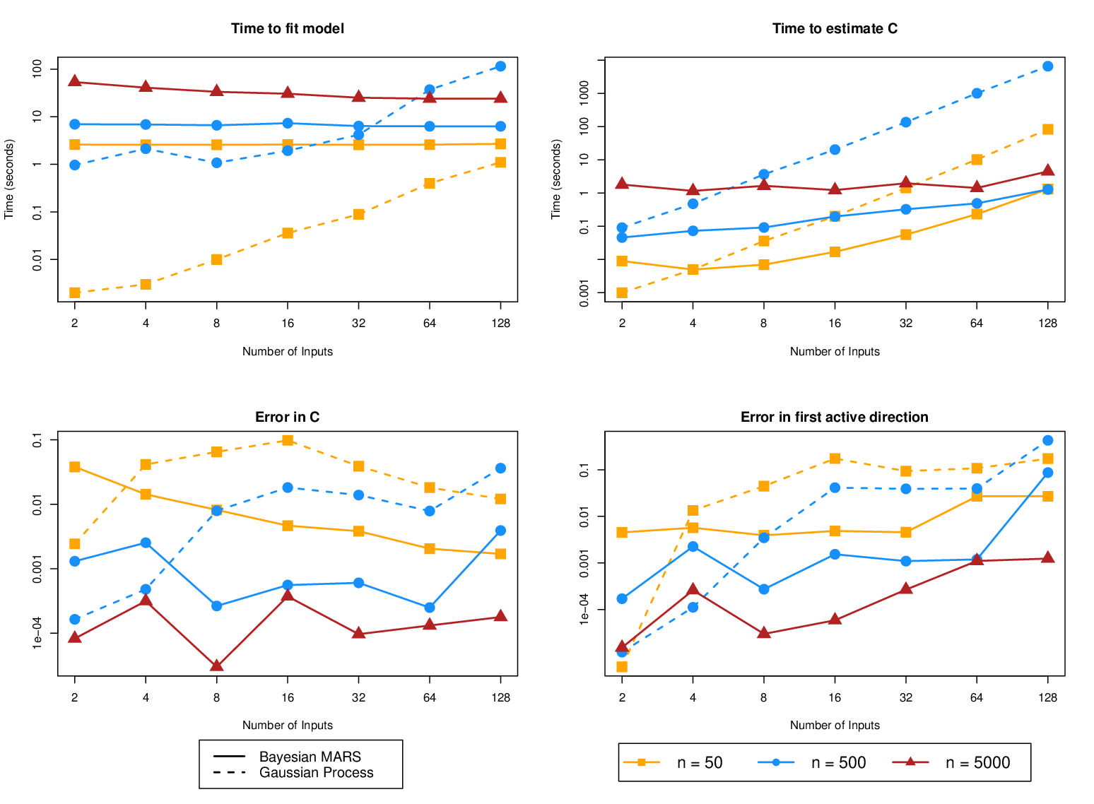
To conduct the analysis, we generate Latin hypercube designs of size , and with dimensions (Note: to reduce variance in the results, a single design is generated for each using and surrogates are fit for each using just the first inputs of each design). The Bayesian MARS surrogate was fit in the open-source R programming language using the BASS::bass() function (Francom & Sansó 2020) and the GP surrogate was fit using the hetGP::mleHomGP() function (Binois & Gramacy 2021). For the respective cases, was estimated using the concordance::C_bass() and activegp::C_GP() functions (Wycoff & Binois 2021).
The results of this simulation study are fully presented in Figure 1. As expected, the computational cost of the GP-surrogate approach drastically increases as either or increase. For example, in the medium-difficulty case with and , the GP based approach required seconds to fit the surrogate and nearly minutes to estimate . For the case where and , we approximate that estimating with the GP-based approach would have taken weeks (for this reason, we did not test the case for GPs at all). The MARS-based approach had much better scaling. For the high-difficulty case with and , we required just seconds to fit the surrogate and seconds to estimate .
For very low-dimensional input spaces (), the GP-based approach led to more precise estimates of both and compared to the MARS approach for equivalent . On the other hand, estimates based on MARS are more accurate for moderate and large ( in some cases, and in all cases). Moreover, the estimators produced by MARS can be improved by adding training data (e.g., see case in Figure 1) while the GP cannot easily take advantage of these additional runs for computational reasons.
4.1.1 A Linear Constraint
Let us again consider the function of Equation 29 (with ), but this time we will assume the existence of the constraint . In particular, suppose we want to find the active subspace of with respect to the prior
| (32) |
which represents a uniform distribution over the lower right half of . As before, we can determine the matrix analytically using Equation 9
| (33) |
This measure cannot be handled directly in our framework because the distribution does not factor into independent components, and no linear transformation of will help here. Instead, we approximate with a mixture of uniform distributions as
| (34) | ||||
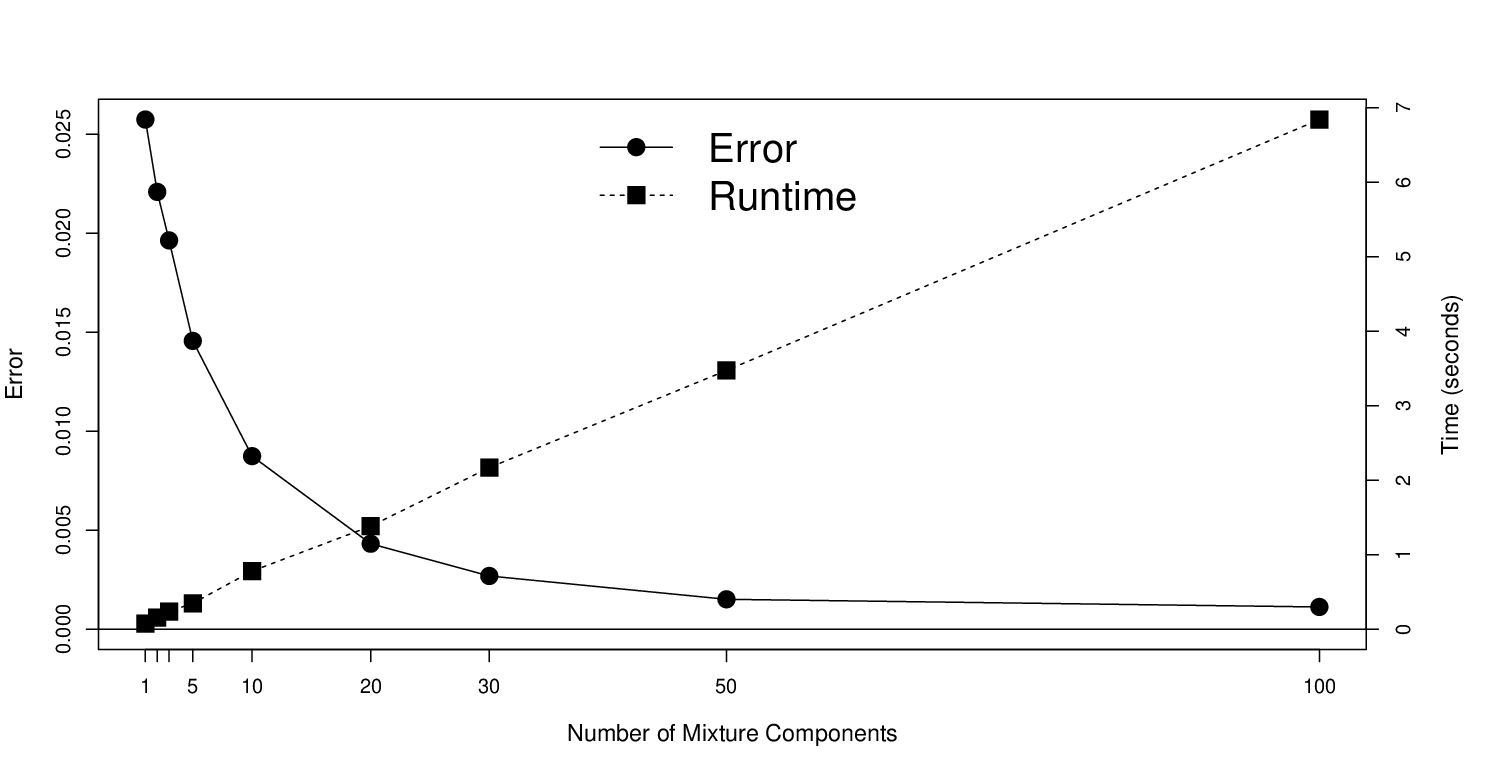
The mixture weights are proportional to the size of each region and are computed as , subject to . From here, is estimated using Equations 20 and 27. Although the accuracy of the approximation improves as grows large, the computation also grows linearly in (though parallel computing can easily offset this cost). Finally, note that for certain constructions, this mixture-based procedure becomes increasingly similar to the standard Monte Carlo approach as . The error of the approximation and the time required are shown as a function of in Figure 2.
Although we perform a similar analysis in a higher-dimension for a real application in Section 4.2, finding a suitable approximation with independent components becomes increasingly difficult as grows and as the constraints become more complex. See Section 4 of the SM for a practical approach.
4.1.2 Capturing Low-Dimensional Structure
We rely on the simple polynomial function one final time to illustrate the low-dimensional structure which can be captured by active subspaces. In this example, take and define a new computer model as

| Active Directions | ||||||
|---|---|---|---|---|---|---|
| 1 | 2 | 3 | 4 | 5 | 6 | |
| Square Root Eigenvalue | ||||||
| Percent of SD Explained | ||||||
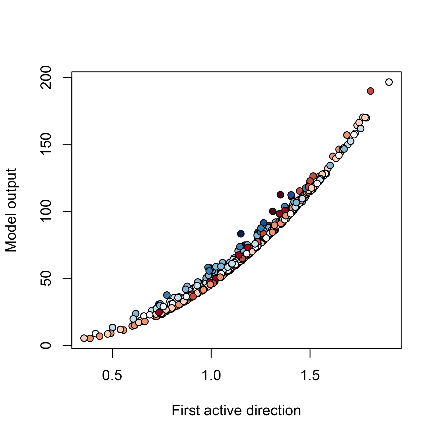
with from Equation 29, and . Next, (i) generate a space filling design over using a Latin hypercube with observations, (ii) fit a Bayesian MARS model to the resulting data and (iii) estimate using our proposed method. Although is a function in dimensions and none of the inputs are inert, the active subspace can be used to construct a lower-dimensional representation of the data. Figure 3(a) shows the non-linear structure that arises when plotting the model output against the data projected onto the first active direction (). Although the one-dimensional structure is apparent, the output cannot be fully explained by just one active direction. Figure 3(b) shows a 3-dimensional scatterplot of against the first two active directions. Note that nearly all of the unexplained variability in is now captured by the reduced data and this is supported by the eigenvalues, shown in Table 1, where the second eigenvalue is not close enough to in magnitude to justify excluding the second active direction. To illustrate further, we fit statistical regression models (Bayesian MARS) for using the -dimensional projection (for ) and calculate the percentage of the standard deviation which is accounted for by the statistical model (see Table 1). Each additional dimension beyond 2 yields diminishing returns for the predictive accuracy of the statistical model.
4.2 A Material Strength Model
In this section, we demonstrate the utility of our approach on an important application in materials science, where we seek to discover the active subspace of a material strength model with respect to two non-trivial input distributions.
The Preston-Tonks-Wallace (PTW) model is a materials strength model which describes the plasticity of a given metal at various temperatures and strain rates (Preston et al. 2003). The equations governing the PTW model are too lengthy to show here, but full details can be found in Fugate et al. 2005 and Price et al. 2013. The PTW model is a complex, highly non-linear function of inputs, corresponding to various material properties, universal constants and measured values. The impact of each input can vary for different metals, temperatures, strain rates and values of the other inputs, so specification of an appropriate measure is of paramount importance.
| Input | Parameter | Lower bound | Upper bound | Description |
|---|---|---|---|---|
| Strain hardening rate | ||||
| Strain hardening constant | ||||
| Saturation stress at K | ||||
| Saturation stress at melting temperature | ||||
| Constant of temperature dependence | ||||
| Constant of strain rate dependence () | ||||
| Yield stress constant at K | ||||
| Yield stress constant at melting temperature | ||||
| Medium strain rate constant | ||||
| Medium strain rate exponent | ||||
| Inert input |
For our purposes, we will use the output of a PTW computer experiment conducted for Ti64, a titanium alloy. The response of interest is the yield stress at a strain of , a temperature of K and a strain rate of per second. Marginal input ranges for each of the parameters are given in Table 2. In addition to these marginal ranges, the PTW model must also respect the constraint
| (35) |
This inequality defines a region which represents the support of . The first measure of interest is the uniform distribution over . Since we cannot compute with respect to this measure directly, we propose to approximate with the union of disjoint hyperrectangles (boxes), and then to approximate with respect to the mixture of uniforms over these boxes.
| (36) | ||||
Each box can be represented by a vector of lower bounds and a vector of upper bounds (). The mixture weights are equal to where . Each component of the mixture can be handled easily using Section 3.3.1 and the combined can be found using Equation 28. To find a suitable approximation , we employ an approach which is inspired by recursive partitioning (Therneau et al. 1997). A detailed description can be found in Section 4 of the SM. The procedure stops when it can no longer recursively add a disjoint hyperrectangle inside of with volume greater than , which leads to an approximation consisting of disjoint boxes.
The second measure of interest is the posterior distribution of the inputs which results from a Bayesian model calibration analysis (Kennedy & O’Hagan 2001). The details are not important here, except that this posterior is unavailable analytically. Instead, we are given a sample of draws from the posterior distribution. To approximate this distribution, we fit a finite mixture of multivariate Gaussian’s using the penalized likelihood approach of Chen & Tan 2009 in combination with the graphical LASSO (Friedman et al. 2008) to induce sparsity. A detailed description of this procedure can be found in Section 5 of the SM. The resulting approximation is a mixture of multivariate Gaussian distributions. The with respect to each mixture component can be found using Equation 24 and the total is found using Equation 28.

To inspect for any potential differences in the active directions with respect to the prior and the posterior, we examine the activity scores (Constantine & Diaz 2017), which are defined for the input parameter as
| (37) |
where is the eigenvalue and is the entry of the eigenvector. Activity scores are a type of global sensitivity metric, with connections to the well-known Sobol index (Sobol 2001). For activity score values to be comparable, we use Theorem to get the matrix for each variable on a scale before obtaining the eigendecomposition. Figure SM4 shows the relative (maximum value of ) activity scores for each of the PTW input parameters with respect to the prior and the calibration posterior. The two measures lead to similar activity scores, indicating the mostly-stationary behavior of the response across the input space. In both cases, the response variable is only sensitive to four inputs with being the most influential parameter. Across the entire (a priori) input space, the variable is the second most influential input. In the a posteriori region of interest, however, the response becomes relatively more sensitive to . For comparison, we also include the active subspace, which is obtained by ignoring the constraints in Equation 15 altogether, and we see that activity due to is overestimated relative to the other variables and the activity with respect to is nearly lost altogether. This analysis shows the sensitivity of active subspace discovery to the specification of the measure and demonstrates the importance of having a method which is compatible with a wide range of appropriate choices for .
4.3 High Dimensional Input: Nuclear Data
Nuclear data characterize the probability of several types of interactions that can occur between atoms. For a particular isotope of an element, the probability of each type of interaction is typically a function of energy and is referred to as a cross section. These cross sections are inputs to codes used to simulate various types of nuclear events, such as the behavior of the nuclear material in a nuclear power plant. Uncertainty in these cross sections, typically parameterized with a multivariate Gaussian distribution, is an important area of research (see chapter 7 of Wu 2019).
In this example, we consider an analysis for which the nuclear data corresponding to a Plutonium isotope are the inputs to a model, and we want to understand the active subspace. More specifically, the inputs are eight cross sections, each discretized into 30 energy bins, which results in 240 inputs (135 of which are non-degenerate and linearly independent). The response is a calculation of criticality (), for which numbers larger than one indicate the multiplication of neutrons (a chain reaction), while values less than one indicate an unsustained reaction. The system of interest is a “critical assembly” known as Jezebel (Sigeti et al. 2018), an experiment used to study criticality of Plutonium, as simulated by a neutron transport code. We have 9372 total simulations, where the 240 dimensional input is generated from the appropriate multivariate Gaussian distribution to reflect underlying uncertainty about the nature of Plutonium (see Sigeti et al. 2018 for more simulation details).
The purpose of this example is to demonstrate our methodology on a challenging (yet realistic) problem. This problem has high input dimension, many model runs and a highly structured correlated prior. The GP based approach of Wycoff et al. 2021 is not at all feasible for this problem and a Monte Carlo based approach will be inefficient given the large input dimension and possibly inaccurate given the lack of well-defined gradients. Prior to this work, the formal active subspace for this computer simulator could not be reasonably and practically obtained, with previous work using the ordinary least squares linear model as a rough proxy (Francom et al. 2019). Using the methods described in this paper with the Bayesian MARS algorithm of (Francom & Sansó 2020), the full active subspace can be discovered using a single core of a 2019 MacBook Pro in under half an hour: seconds to fit the Bayesian MARS model and minutes to compute the matrix.

We briefly summarize the steps required to find the active subspace. Given the prior mean and covariance matrix , we transform the data as . Since the induced prior for is now standard normal, we can use Equation 16 from Section 3.3.1 to estimate . Finally, we use Theorem 2 and Equation 24 to obtain the matrix with respect to the original inputs and obtain the eigendecomposition of this matrix to reveal the active subspace. The left panel of Figure 5 shows the eigenvalues for the linearly independent inputs. Using a sequential testing procedure (Ma & Zhu 2013), and are found to be reasonable choices for the reduced dimension of the active subspace. The right panel of Figure 5 represents the data, projected onto the first active direction, against the response variable. The fit is exceptionally good, which agrees with previous work which demonstrated the simple linear model adequately emulated the simulator across the input region of interest.
Finally, we comment on another practical benefit of this procedure. For this computationally intensive dataset, the Bayesian MARS model took seconds to run, required up to basis functions, and performed no better than a simple linear model. After projecting the original data onto the active directions that were discovered, the Bayesian MARS model which is fit to the projected data took just seconds to run, required just basis functions (leading to a more memory-efficient model) and outperformed both the linear model and the first BMARS model by an order of magnitude (with respect to RMSE).
5 Conclusion
In this work, we discuss the limitations of current methodologies for the discovery of active subspaces for computer models with high dimensional inputs and we propose an alternative approach which is designed for these cases. The new approach is fast and highly accurate, even when a large number of observations are required to capture the full behavior of the computer model. In small sample or small input dimension problems, our approach is still competitive with an existing method based on Gaussian processes (Wycoff et al. 2021). Though our development focuses on the use of MARS or Bayesian MARS models as a surrogate, the results in Section 3.1 are general enough to recover the GP based solution and can be applied to other surrogate methods including radial basis regression. We have also provided, to date, the most comprehensive discussion of the measure on which the active subspace depends. The new approach is flexible enough to handle univariate measures including beta, gamma and truncated normal distributions, and can also treat more sophisticated measures such as a mixture of multivariate normal distributions. This flexibility handles important special cases, such as prior distributions with physical constraints on the input space and posterior distributions which are represented as a set of finite samples (e.g., calibration). This work can be extended by developing equations for sequential computer experiment design, such as in Wycoff et al. 2021. It is also possible to develop a robustness procedure for the estimation of , by repeating the analysis on the projected data and using Theorem 2 until the active subspace converges. This can complicated because the measure corresponding to the projected variables is a high dimensional composition of the measure for and dependence among the projected variables will be introduced. For similar reasons, producing the relevant calculations for neural network surrogates (Tripathy & Bilionis 2018) represents a highly-challenging yet valuable opportunity for future work. Lastly, as shown in Section 4.3, the active directions can be leveraged to create a new Bayesian MARS model which is both (i) more accurate and (ii) more memory efficient than the model based on the native input space. This suggests that a projected Bayesian MARS algorithm, with similarities to neural networks (Mao & Jain 1995) and Bayesian projection pursuit (Collins et al. 2022), may be a valuable tool for nonparametric regression and computer model emulation.
References
- (1)
- Batta et al. (2021) Batta, I., Abrol, A. & Calhoun, V. (2021), Uncovering active structural subspaces associated with changes in indicators for alzheimer’s disease, in ‘2021 43rd Annual International Conference of the IEEE Engineering in Medicine & Biology Society (EMBC)’, IEEE, pp. 3948–3951.
- Berger (1990) Berger, J. O. (1990), ‘Robust Bayesian analysis: sensitivity to the prior’, Journal of statistical planning and inference 25(3), 303–328.
- Bierens (1987) Bierens, H. J. (1987), Kernel estimators of regression functions, in ‘Advances in econometrics: Fifth world congress’, Vol. 1, pp. 99–144.
- Binois & Gramacy (2021) Binois, M. & Gramacy, R. B. (2021), ‘hetgp: Heteroskedastic Gaussian process modeling and sequential design in R’, Journal of Statistical Software 98, 1–44.
- Chen & Tan (2009) Chen, J. & Tan, X. (2009), ‘Inference for multivariate normal mixtures’, Journal of Multivariate Analysis 100(7), 1367–1383.
- Chen et al. (2005) Chen, W., Jin, R. & Sudjianto, A. (2005), ‘Analytical variance-based global sensitivity analysis in simulation-based design under uncertainty’, Journal of mechanical design 127(5), 875–886.
- Claeskens et al. (2008) Claeskens, G., Hjort, N. L. et al. (2008), ‘Model selection and model averaging’, Cambridge Books .
- Collins et al. (2022) Collins, G., Francom, D. & Rumsey, K. (2022), ‘Bayesian projection pursuit regression’, arXiv preprint arXiv:2210.09181 .
- Constantine (2015) Constantine, P. G. (2015), Active subspaces: Emerging ideas for dimension reduction in parameter studies, SIAM.
- Constantine & Diaz (2017) Constantine, P. G. & Diaz, P. (2017), ‘Global sensitivity metrics from active subspaces’, Reliability Engineering & System Safety 162, 1–13.
- Constantine & Doostan (2017) Constantine, P. G. & Doostan, A. (2017), ‘Time-dependent global sensitivity analysis with active subspaces for a lithium ion battery model’, Statistical Analysis and Data Mining: The ASA Data Science Journal 10(5), 243–262.
- Constantine et al. (2014) Constantine, P. G., Dow, E. & Wang, Q. (2014), ‘Active subspace methods in theory and practice: applications to kriging surfaces’, SIAM Journal on Scientific Computing 36(4), A1500–A1524.
- Constantine et al. (2016) Constantine, P. G., Kent, C. & Bui-Thanh, T. (2016), ‘Accelerating Markov chain Monte Carlo with active subspaces’, SIAM Journal on Scientific Computing 38(5), A2779–A2805.
- Constantine et al. (2015) Constantine, P. G., Zaharatos, B. & Campanelli, M. (2015), ‘Discovering an active subspace in a single-diode solar cell model’, Statistical Analysis and Data Mining: The ASA Data Science Journal 8(5-6), 264–273.
- Datta & Ghosh (2014) Datta, J. & Ghosh, J. K. (2014), ‘Bootstrap—an exploration’, Statistical Methodology 20, 63–72.
- Denison et al. (1998) Denison, D. G., Mallick, B. K. & Smith, A. F. (1998), ‘Bayesian MARS’, Statistics and Computing 8(4), 337–346.
- Domingos (2012) Domingos, P. (2012), ‘A few useful things to know about machine learning’, Communications of the ACM 55(10), 78–87.
- Fernandez-de Cossio-Diaz (2017) Fernandez-de Cossio-Diaz, J. (2017), ‘Truncatednormal.jl’, https://github.com/cossio/TruncatedNormal.jl.
- Francom et al. (2019) Francom, D. C., Vander Wiel, S. A. & Weaver, B. P. (2019), Nuclear data dimension reduction, Technical report, Los Alamos National Lab.(LANL), Los Alamos, NM (United States).
- Francom & Sansó (2020) Francom, D. & Sansó, B. (2020), ‘BASS: An R package for fitting and performing sensitivity analysis of Bayesian adaptive spline surfaces’, Journal of Statistical Software 94(1), 1–36.
- Friedman (1991) Friedman, J. H. (1991), ‘Multivariate adaptive regression splines’, The annals of statistics pp. 1–67.
- Friedman & Meulman (2003) Friedman, J. H. & Meulman, J. J. (2003), ‘Multiple additive regression trees with application in epidemiology’, Statistics in medicine 22(9), 1365–1381.
- Friedman & Stuetzle (1981) Friedman, J. H. & Stuetzle, W. (1981), ‘Projection pursuit regression’, Journal of the American statistical Association 76(376), 817–823.
- Friedman et al. (2008) Friedman, J., Hastie, T. & Tibshirani, R. (2008), ‘Sparse inverse covariance estimation with the graphical lasso’, Biostatistics 9(3), 432–441.
- Fugate et al. (2005) Fugate, M., Williams, B., Higdon, D., Hanson, K. M., Gattiker, J., Chen, S.-R. & Unal, C. (2005), ‘Hierarchical Bayesian analysis and the Preston-Tonks-Wallace model’, Los Alamos National Laboratory Technical Report LA-UR-05-3935 .
- Gramacy (2020) Gramacy, R. B. (2020), Surrogates: Gaussian process modeling, design, and optimization for the applied sciences, CRC press.
- Härdle & Stoker (1989) Härdle, W. & Stoker, T. M. (1989), ‘Investigating smooth multiple regression by the method of average derivatives’, Journal of the American statistical Association 84(408), 986–995.
- Hielscher et al. (2018) Hielscher, T., Niemann, U., Preim, B., Völzke, H., Ittermann, T. & Spiliopoulou, M. (2018), ‘A framework for expert-driven subpopulation discovery and evaluation using subspace clustering for epidemiological data’, Expert Systems with Applications 113, 147–160.
- Higdon (2002) Higdon, D. (2002), Space and space-time modeling using process convolutions, in ‘Quantitative methods for current environmental issues’, Springer, pp. 37–56.
- Jefferson et al. (2015) Jefferson, J. L., Gilbert, J. M., Constantine, P. G. & Maxwell, R. M. (2015), ‘Active subspaces for sensitivity analysis and dimension reduction of an integrated hydrologic model’, Computers & geosciences 83, 127–138.
- Ji et al. (2019) Ji, W., Ren, Z., Marzouk, Y. & Law, C. K. (2019), ‘Quantifying kinetic uncertainty in turbulent combustion simulations using active subspaces’, Proceedings of the Combustion Institute 37(2), 2175–2182.
- Kennedy & O’Hagan (2001) Kennedy, M. C. & O’Hagan, A. (2001), ‘Bayesian calibration of computer models’, Journal of the Royal Statistical Society: Series B (Statistical Methodology) 63(3), 425–464.
- Li (1991) Li, K.-C. (1991), ‘Sliced inverse regression for dimension reduction’, Journal of the American Statistical Association 86(414), 316–327.
- Lin & Unbehauen (1992) Lin, J.-N. & Unbehauen, R. (1992), ‘Canonical piecewise-linear approximations’, IEEE Transactions on Circuits and Systems I: Fundamental Theory and Applications 39(8), 697–699.
- Lukaczyk et al. (2014) Lukaczyk, T. W., Constantine, P., Palacios, F. & Alonso, J. J. (2014), Active subspaces for shape optimization, in ‘10th AIAA multidisciplinary design optimization conference’, p. 1171.
- Ma & Zhu (2013) Ma, Y. & Zhu, L. (2013), ‘A review on dimension reduction’, International Statistical Review 81(1), 134–150.
- Mao & Jain (1995) Mao, J. & Jain, A. K. (1995), ‘Artificial neural networks for feature extraction and multivariate data projection’, IEEE transactions on neural networks 6(2), 296–317.
- Mishra (2012) Mishra, B. (2012), Algorithmic algebra, Springer Science & Business Media.
- Navaneeth & Chakraborty (2022) Navaneeth, N. & Chakraborty, S. (2022), ‘Surrogate assisted active subspace and active subspace assisted surrogate—a new paradigm for high dimensional structural reliability analysis’, Computer Methods in Applied Mechanics and Engineering 389, 114374.
- Othmer et al. (2016) Othmer, C., Lukaczyk, T. W., Constantine, P. & Alonso, J. J. (2016), On active subspaces in car aerodynamics, in ‘17th AIAA/ISSMO Multidisciplinary Analysis and Optimization Conference’, p. 4294.
- Park (1994) Park, J.-S. (1994), ‘Optimal Latin-hypercube designs for computer experiments’, Journal of statistical planning and inference 39(1), 95–111.
- Park & Sandberg (1993) Park, J. & Sandberg, I. W. (1993), ‘Approximation and radial-basis-function networks’, Neural computation 5(2), 305–316.
- Preston et al. (2003) Preston, D. L., Tonks, D. L. & Wallace, D. C. (2003), ‘Model of plastic deformation for extreme loading conditions’, Journal of applied physics 93(1), 211–220.
- Price et al. (2013) Price, M. C., Kearsley, A. T. & Burchell, M. J. (2013), ‘Validation of the Preston–Tonks–Wallace strength model at strain rates approaching 1011 s- 1 for Al-1100, tantalum and copper using hypervelocity impact crater morphologies’, International Journal of Impact Engineering 52, 1–10.
- Redner & Walker (1984) Redner, R. A. & Walker, H. F. (1984), ‘Mixture densities, maximum likelihood and the EM algorithm’, SIAM review 26(2), 195–239.
- Rumsey et al. (2023) Rumsey, K., Francom, D. & Shen, A. (2023), ‘Generalized bayesian mars: Tools for emulating stochastic computer models’, arXiv preprint arXiv:2306.01911 .
- Seshadri et al. (2018) Seshadri, P., Shahpar, S., Constantine, P., Parks, G. & Adams, M. (2018), ‘Turbomachinery active subspace performance maps’, Journal of Turbomachinery 140(4).
- Shekhtman (1982) Shekhtman, B. (1982), ‘Why piecewise linear functions are dense in cio, 1’, Journal of Approximation Theory 36, 265–267.
- Sigeti et al. (2018) Sigeti, D. E., Parsons, D. K., White, M. C., Francom, D. C., Vander Wiel, S. A., Weaver, B. P. & Williams, B. J. (2018), ENDF/B-VIIIrc1 239Pu Uncertainties: Constraints, Sampling, and Calibration to Jezebel, Technical report, Los Alamos National Lab.(LANL), Los Alamos, NM (United States).
- Sobol (2001) Sobol, I. M. (2001), ‘Global sensitivity indices for nonlinear mathematical models and their Monte Carlo estimates’, Mathematics and computers in simulation 55(1-3), 271–280.
- Tezzele et al. (2018) Tezzele, M., Ballarin, F. & Rozza, G. (2018), Combined parameter and model reduction of cardiovascular problems by means of active subspaces and pod-galerkin methods, in ‘Mathematical and numerical modeling of the cardiovascular system and applications’, Springer, pp. 185–207.
- Therneau et al. (1997) Therneau, T. M., Atkinson, E. J. et al. (1997), An introduction to recursive partitioning using the RPART routines, Technical report, Technical report Mayo Foundation.
- Tripathy & Bilionis (2018) Tripathy, R. K. & Bilionis, I. (2018), ‘Deep UQ: Learning deep neural network surrogate models for high dimensional uncertainty quantification’, Journal of computational physics 375, 565–588.
- Vohra et al. (2019) Vohra, M., Alexanderian, A., Guy, H. & Mahadevan, S. (2019), ‘Active subspace-based dimension reduction for chemical kinetics applications with epistemic uncertainty’, Combustion and Flame 204, 152–161.
- Wu (2019) Wu, Y. (2019), Neutronics of Advanced Nuclear Systems, Springer.
- Wycoff & Binois (2021)
Wycoff, N. & Binois, M. (2021),
activegp: Gaussian Process Based Design and Analysis for the Active
Subspace Method.
R package version 1.0.6.
https://CRAN.R-project.org/package=activegp - Wycoff et al. (2021) Wycoff, N., Binois, M. & Wild, S. M. (2021), ‘Sequential learning of active subspaces’, Journal of Computational and Graphical Statistics 30(4), 1224–1237.
- Xia (2008) Xia, Y. (2008), ‘A multiple-index model and dimension reduction’, Journal of the American Statistical Association 103(484), 1631–1640.
- Xu et al. (2009) Xu, J., Huang, X. & Wang, S. (2009), ‘Adaptive hinging hyperplanes and its applications in dynamic system identification’, Automatica 45(10), 2325–2332.
Supplemental Materials: Discovering Active Subspaces for High Dimensional Computer Models
6 Estimate C - Pseudocode
7 Proof of Theorem 1
Theorem 2
Let and take . If is invertible, then we have
where is the matrix taken with respect to and and is taken with respect to and .
Proof:
Let be a function of the form shown in Equation (6) of the main text and take . Then
Therefore, the matrix for can be written in terms of the matrix for as follows.

8 Additional Examples
8.1 Simple Polynomial with Corrupted Data
Consider again the simple polynomial function from Section 4.1
and suppose that we are given training data
Here, represents a “corruption mechanism” which has perturbed the response for of the observations. In this example, we seek to explore the impact of these outliers on our ability to estimate across various methods. We will show that estimates of based on GPs (Wycoff et al. 2021) and those based on standard Gaussian BMARS (Francom & Sansó 2020) will be negatively affected by this process. Using a Bayesian MARS model under a -likelihood, as explored in Rumsey et al. 2023, can lead to better estimates of and will result in better estimates of the active subspace. This generalized BMARS approach is compatible with the methods described in this manuscript without requiring any modifications. Code to reproduce this example can be found at https://github.com/knrumsey/ASM-BMARS-Examples.
Setting , we simulate different sets of training data using the process described above and we estimate using a GP, BASS and TBASS() surrogate. The quality of the estimate of is measured with the Frobenius norm, and the results are given in Table 1. The TBASS method is the clear winner, by about an order of magnitude. Figure SM1 gives kernel density estimates for the difference in Frobenius norm across the simulations.
| BASS | TBASS | GP | |
|---|---|---|---|
| Min. | |||
| 1st Qu. | |||
| Median | |||
| Mean | |||
| 3rd Qu. | |||
| Max. |
8.2 Additional Example: Global Sensitivity Analysis for Stochastic SIR Model
By estimating conditional on a MARS model, we are able to take advantage of the flexible-likelihoods offered by generalized Bayesian MARS (Rumsey et al. 2023). In this example, we will recreate the example found in Section 4.3 of Rumsey et al. 2023 for activity scores (rather than Sobol effects, as in the cited paper). For a detailed description of the problem, we defer to Rumsey et al. 2023.
Briefly, we take to be a stochastic SIR model with inputs and we fit a series of quantile regression BASS models for various quantiles . We can now assess the sensitivity using activity scores (Constantine 2015) for each quantile. Much can be learned about a computer model by studying how the sensitivity to its various inputs changes as a function of quantiles. The results of this simulation can be seen in Figure SM2. Code to reproduce this example can be found at https://github.com/knrumsey/ASM-BMARS-Examples.

8.3 Uncertainty Quantification for Activity Scores
One advantage of the methods described in this paper, compared to the GP-based approach, is that the posterior uncertainty of the surrogate model fit can be propagated forward to the estimate of the active subspace. In this example, we return again to the simple polynomial function of Section 4.1. With and , we fit a BASS model which can be viewed as a posterior ensemble of various MARS models, one for each MCMC iteration. We can find the matrix corresponding to each MARS model. By computing the activity scores (Constantine 2015) for each , we obtain posterior distributions for these quantities. Figure SM3 shows the posterior distribution of the activity scores (as boxplots) alongside the point estimate produced by the GP-based approach. Code to reproduce this example can be found at https://github.com/knrumsey/ASM-BMARS-Examples.

9 Details of recursive partitioning algorithm
We begin by finding the minimal rectangle which contains , call it , which is fully defined by the spanning each of the coordinates. We then split along one of it’s dimensions forming two new boxes and such that
and , for , where . We then check (separately) to see if and is either (i) entirely contained in , (ii) entirely contained outside of or (iii) partially contained in . In the first case, we terminate and return the box. In the second case, we terminate without returning anything and in the final case we recursively repeat the procedure, treating the box (or ) as a new and using a new splitting dimension .
This procedure requires that we can quickly check whether a box lives inside, outside or overlaps the region . If is concave, as is it is in the PTW model, then it is sufficient to check if each of the vertices is in (with at least one vertex required to be in the interior of , for to be considered entirely contained). There is also some freedom in the mechanism for choosing the splitting dimension . For instance, in the PTW example, we only split over variables and and we iterate between these dimensions at each level of recursion (similarly, we need only check the vertices corresponding to these inputs, rather than the full ). Finally, we note that this procedure will converge to (under Lesbesgue measure) for regions which can be defined by a set of linear inequalities (Mishra 2012), and so a reasonable stopping criteria is needed. One sensible choice is to stop recursing when the rectangle volume is below a pre-specified threshold.
Using this procedure for the PTW model with the bounds given in Table 2 (main text), the constraint in Equation 35 (main text) and a minimum box volume of , we were able to generate an approximation consisting of disjoint boxes. These boxes cover only about of the constrained space by volume, but volume is a highly misleading measure in high dimensions. This is an unsurprising result, since volume in high dimensions is concentrated around the boundary (”nearly all the volume in a high dimensional orange is in the peel” (Domingos 2012)) and the recursive method described here fails to fill in edges of the space, because the boxes required for ”squeezing” into corners are smaller than the tolerance. By lowering the tolerance to , we obtain an approximation consisting of boxes which covers of the space by volume.
10 Details of multivariate normal mixture fitting
For the PTW example, we are given draws from the -dimensional posterior distribution. Since fitting mixtures of multivariate Gaussian distributions is a computationally demanding and difficult problem, we start by reducing the dimension of the mixture from to just the dimensions that are involved with the PTW constraint in Equation 35. This choice was supported via the graphical LASSO approach of Friedman et al. 2008 and the bootstrap as applied in Section 2 of Datta & Ghosh 2014. Both approaches suggest that the remaining inputs (those not included in the constraint) can be treated as independent.

From here we apply the robust penalized EM algorithm of Chen & Tan 2009, which shrinks the MLE of the covariance matrix towards the sample covariance matrix. We use a small penalty term for robustness, corresponding to () in Chen & Tan 2009. The log-likelihood grows roughly linearly with the number of components (from to ). The rate of growth is such that the Bayesian information criterion (BIC) suggests a standard multivariate Gaussian is appropriate and Akaike’s information criterion (AIC) suggests mixture components. On the other hand, the Hannan-Quinn information criterion (HQIC) repeatedly (running multiple experiments to reduce convergence error) prefers mixture components, although it largely agrees with BIC. Claeskens et al. 2008 discuss the advantages of HQIC, which include strong consistency (unlike AIC) and near asymptotic efficiency (unlike BIC, missing optimal convergence by a very small factor). Monte Carlo suggests that this 2-component mixture of multivariate Gaussians has about of it’s density inside the constraints of Equation 15 (main text). The two component mixture that we select for inputs is given by its parameters
| (SM1) | ||||
and the remaining inputs are fitted with independent univariate normal distributions.
11 Propagation of Model Uncertainty with Bayesian MARS
For all of the results in this paper, we construct surrogate models using the Bayesian MARS algorithm of (Francom & Sansó 2020). One advantage of Bayesian MARS is that the posterior distribution of the model parameters essentially yields an ensemble of MARS models. By computing the active subspace for each model in the ensemble, we can (i) improve the final estimate of the active subspace and (ii) characterize the uncertainty in the estimate that comes from the model fitting procedure. This comes at a cost of course, since the matrix must be constructed times, where is the number of samples from the posterior distribution. For large complex problems, constructing may be fast, but if is large, the ensemble can take a long time to process.
In order to leverage the structure of the Bayesian MARS posterior sampler, we first write
| (SM2) |
where represents the (elementwise) Hadamard product. This formula provides a convenient way to compute each element of quickly, and in terms of the matrices and .
Through close examination of the sampling procedure used in Bayesian MARS, we can find opportunities for substantial time savings. Using memory, we can reuse much of work from one iteration to the next. In particular, the model changes only slightly and in a very structured way from one iteration to another. The model at iteration differs from the model at iteration in one of four ways:
- •
Birth. One basis function is added to the model at iteration . Thus, we must add a column and row, corresponding to this new basis function, for each matrix. We can then re-compute using Equation SM2.
- •
Death. One basis function has been removed from the model at iteration . If the basis function was deleted, then we simply delete the row and column from each matrix.
- •
Mutation. One basis function has been altered at iteration . If the basis function was altered, then we need to recompute the row and column of each matrix.
- •
Rejection. No modification was accepted during iteration . The model is the same, except for the regression coefficients which have been resampled. In this case, we simply use Equation SM2 with the new values for .
Since evaluating integrals is the primary consumer of resources in our estimation procedure, it is clear that there are substantial time-savings to be had. In the case of a birth and a mutation, only integrals must be evaluated compared to integrals when computing from scratch. During a death or rejection step, we avoid computing new integrals altogether.
12 Time and Memory Tradeoff
As a brief aside, we also note that when and are very large, we can trade memory for time by storing the matrix and making the approximations
| (SM3) | ||||
where is a small positive number, is a matrix of ones and denotes Hadamard division.
13 The Effect of Interaction Order on Estimation of C
Consider a modified simple polynomial function with a three-variable interaction present
We simulate data for input variables with and fit a series of BASS models with and . We also fit with a BASS model with the birth.type="coinflip" option, which effectively sets . Table 2 gives the out-of-sample RMSPE for each model and the error in estimating (the true value of is estimated via Monte Carlo with million MC samples). We note that the concordance package cannot estimate in the case where maxInt = 1.
| maxInt = 1 | maxInt = 2 | maxInt = 3 | maxInt = 4 | coinflip | |
|---|---|---|---|---|---|
| RMSPE | |||||
| Error |
The best results come from the case where , which is the true maximum interaction order of the function . The second best case is the BASS model fit with the “coinflipping” birth type, which we propose as a reasonable default when the true interaction order of the model is unknown.