Mixing Sinc kernels to improve interpolations in smoothed particle hydrodynamics without pairing instability2023Mixing Sinc kernels to improve interpolations in smoothed particle hydrodynamics without pairing instability–References
Abstract
The smoothed particle hydrodynamic technique is strongly based on the proper choice of interpolation functions. This statement is particularly relevant for the study of subsonic fluxes and turbulence, where inherent small errors in the averaging procedures introduce excessive damping on the smallest scales. To mitigate these errors we can increase both the number of interpolating points and the order of the interpolating kernel function. However, this approach leads to a higher computational burden across all fluid regions. Ideally, the development of a single kernel function capable of effectively accommodating varying numbers of interpolating points in different fluid regions, providing good resolution and minimal errors would be highly desirable. In this work, we revisit and extend the main properties of a family of interpolators called Sinc kernels and compare them with the widely used family of Wendland kernels. We show that a linear combination of low- and high-order Sinc kernels generates good-quality interpolators, which are resistant to pairing instability while maintaining good sampling properties in a wide range of neighbor interpolating points, . We show that a particular case of this linear mix of Sincs produces a well-balanced and robust kernel that improves previous results in the Gresho-Chan vortex experiment even when the number of neighbors is not large, while yielding a good convergence rate. Although such a mixing technique is ideally suited for Sinc kernels owing to their excellent flexibility, it can be easily applied to other interpolating families such as the B-splines and Wendland kernels.
Keywords:
methods: numerical – hydrodynamics1 Introduction
Despite the enormous progress made by the smoothed particle hydrodynamics (SPH) method since it was formulated (Lucy 1977; Gingold & Monaghan 1977) there is still room for improvement in different areas. Among them, convergence issues are of utmost importance. Especially if we want to grasp fine details in fluid-dynamics studies, such as numerically reproducing three-dimensional turbulence (Price et al. 2018). In SPH, the best approach is to use a Lagrangian-compatible formulation Springel & Hernquist 2002 plus a large number of particles and neighbors (Zhu et al. 2015), the two latter being limited by the available computational resources. However, details matter, such as how gradient estimation is implemented (either traditional (Monaghan 1992; Price 2012), least squares (Dilts 1999), or integral (García-Senz et al. 2012) approaches) and the quality of the interpolating kernel (Fulk & Quinn 1996; Rosswog 2015).
Traditionally, the SPH technique has made use of the B-splines family of polynomials, , to carry out the interpolations that are at the foundation of the method. This is a well-justified choice because these kernels have compact support, are fast to compute, and have some flexibility in the choice of the interpolating polynomial, going from the widely used cubic spline to higher-order () polynomials. The family has a support interval that is not the same among all the kernels, being larger for higher-degree polynomials. As a consequence, the number of neighbors allocated within has to increase as increases, to keep a good sampling of the fluid when interpolating. Otherwise, the scarcity of neighbor particles close to the center of the kernel makes the density estimation too dependent on the particle self-contribution, then inducing what is commonly known as bias (Dehnen & Aly 2012; Rosswog 2015; Price et al. 2018). Furthermore, the family has a nonpositive Fourier transform , where is the number of dimensions. As a consequence, they can fall prey to the so-called pairing (or clustering) instability when the number of neighbors is high. The existence of the pairing instability was first noted by Schuessler & Schmitt 1981 who realized that above a critical number of neighbor particles, many compact-supported kernels tend to produce an artificial particle clumping, which not only degrades the effective resolution but produces nonphysical gradients of pressure.
A different family of polynomials , based on Wendland functions Wendland 1995 and more resistant to the pairing instability, was fully discussed by Dehnen & Aly 2012 in the context of the SPH technique. Unlike the family, these (or Wendland) kernels have , where is the wavenumber. Nevertheless, its practical execution demands taking a high number of neighbors to elude bias. However, increasing the number of neighbors raises the computational effort considerably, not only in terms of the number of operations per particle but also in terms of communications overhead in massively distributed calculations.
Finally, another kind of interpolator is the Sinc kernel family, (Cabezón et al. 2008; García-Senz et al. 2014), directly linked to the Dirac- function. These are a very flexible uniparametric family of interpolators steered by the kernel exponent , with similar properties as the B-splines family. Although oscillates around zero, an appropriate choice of the exponent shifts to high wavenumbers, thus suppressing the pairing instability in practice.
In this work we discuss more deeply the properties of the family of kernels proposed in (Cabezón et al. 2008), with emphasis on the connections between the value of the governing exponent of the kernel, its Fourier transform , and the quality of the sampling. We show that combining linearly two kernels with different exponents gives rise to interpolators that are even more resistant to particle clustering while retaining good sampling properties. A correct sampling also helps to control the so-called E0 errors which in SPH appear whenever the integrals defining the average of physical magnitudes and its gradients are approached by finite summations (Monaghan 2005). These E0 errors result in SPH not achieving complete second-order accuracy. Nevertheless, they can be minimized by a correct choice of the interpolation kernel and by increasing the number of interpolating points. The suggested linear mix of low- and high-order kernels can be used either when the number of interpolating neighbor particles is small, allowing for higher spatial resolution with less computational effort, or if the number of neighbors is large, reducing the E0 errors without suffering undesirable particle clustering.
Our main objective is therefore to build a general-purpose kernel able to handle an ample range of neighbor particles without suffering from particle clustering and with good sampling properties. According to our numerical experiments, mixing two Sinc kernels can achieve this result while still rivaling the best results obtained with several members of the family of polynomials. But unlike the or kernel families, our default mixed Sinc kernel does not require a previous and careful choice of the kernel order as a function of the chosen number of target neighbors. For example, our study suggests that the Wendland behaves better than and when the number of neighbors is low or moderate, , but it is recommended to turn it to and progressively in the interval . As we will see, this shortcoming is outpowered by the novel interpolator proposed in this work, with no additional inconveniences.
The main properties of Sinc and mixed Sinc kernels are reviewed in Sects. 2 and 3. Section 4 presents tests that highlight the ability of mixed Sinc kernels to accurately reproduce the density profile in a uniform system (Sect. 4.1), to overcome the pairing-instability, (Sect. 4.2), and to handle the Gresho-Chan vortex experiment (Sect. 4.3) and the Sod shock-tube test (Sect. 4.4). We summarize the main results of our work and provide some guidelines for future work in the Conclusions Section.
2 Properties of the Sinc kernels
The Sinc interpolation family, , was first proposed by Cabezón et al. 2008 as a practical and flexible way to switch between interpolators of different widths and sharpness with a single parameter. They are spherically symmetric functions that come directly from one of the numerical representations of a Dirac- function (Cabezón et al. 2017),
| (1) |
where is a normalization constant, is the particle-neighbor distance normalized to the local smoothing length , and is the kernel index. The family has compact support in , defined in the interval with radius11 1 The radius is defined as the distance to the kernel center at which and . , and its main features have been described in (Cabezón et al. 2008; García-Senz et al. 2014; Cabezón et al. 2017; Rosswog 2015). One of the aims of the original work was to suppress the pairing instability by simply raising the value of the kernel exponent. Increasing makes the kernel sharper, thus shifting to low values. It turns out that raising the index of the kernel also pushes to high wave numbers, which hinders particle clustering.
| FWHM | |||||
| 3 | 0.540 | 1.080 | 1.852 | 1.468 | 0.840 |
| 4 | 0.487 | 0.973 | 2.055 | 1.276 | 1.029 |
| 5 | 0.446 | 0.892 | 2.242 | 1.148 | 1.224 |
| 6 | 0.414 | 0.828 | 2.415 | 1.048 | 1.425 |
| 7 | 0.388 | 0.776 | 2.579 | 0.972 | 1.638 |
| 8 | 0.366 | 0.732 | 2.732 | 0.912 | 1.860 |
| 9 | 0.348 | 0.696 | 2.877 | 0.860 | 2.304 |
| Mixed | FWHM | ||||
| 0.475 | 0.950 | 2.105 | 1.152 | 1.935 | |
| 0.437 | 0.874 | 2.288 | 1.080 | 2.082 | |
| 0.427 | 0.854 | 2.342 | 1.080 | 1.680 | |
| FWHM | |||||
| 2 | 0.516 | 1.032 | 1.938 | 1.256 | - |
| 4 | 0.354 | 0.708 | 2.829 | 1.124 | - |
| 6 | 0.261 | 0.522 | 3.830 | 1.012 | - |
Table 1 shows several features of the and families with compact support , such as the standard deviation,


| (2) |
and the distance (roughly at a half of ) that is often taken as the effective smoothing length (Dehnen & Aly 2012). The last column shows the full width at half maximum (FWHM) of the kernels, which we found is a useful parameter to make comparisons among them. For example, the properties of the interpolator shown in Table 1 are close to those of the cubic spline, , kernel. It has the same support interval and similar and FWHM values. A comparison between the , , and profiles in (Cabezón et al. 2017) suggests the following rough analogy: and , respectively. The similarity between these Sinc and Wendlands interpolators on a purely morphological basis is also supported by the similarity among their FWHM values, as shown in the fifth column of Table 1. Nevertheless, a second parameter related to the Fourier Transform (FT) of the interpolating function is also necessary to better characterize kernels. This is because, despite having similar shapes, their FT can be very different and, more specifically, its behavior at a large wavenumber.

| (3) |
where is a spherically symmetric kernel and is the wavenumber in the three-dimensional space. We show the Fourier transforms of several kernels, in the range calculated with Eq. (3) in the left panel of Fig. 1. As noted in previous works (García-Senz et al. 2014; Cabezón et al. 2017), remains positive at long wavenumber when is high but begins to oscillate around zero after a critical wavenumber , which we show for several kernels in the last column of Table 1. Therefore, the FT of the family is non-positive definite. We also show in the same panel of Fig. 1 the FT of the polynomial that oscillates strongly after . Nevertheless, high-order kernels and manage to shift to higher wavenumbers so that they behave, in practice, closer to kernels with positive-definite Fourier transform. For instance, according to Fig. 1 (left panel), the interpolator remains positive in a range of wavelengths that nearly triples that of . On another note, the family is constructed to have for all wavenumbers (right panel of Fig. 1). Because avoiding artificial particle clustering (i.e., pairing instability) is bounded to a positive FT of the kernel (Dehnen & Aly 2012), the polynomials have become very popular in the field, especially when using a large number of neighbor particles. The central panel of Fig. 1 shows the effect of mixing Sinc kernels on the shape of the FT, pushing towards larger wavenumbers. This will be discussed in more detail in Sect. 3.
The other side of the coin is that high-order kernels of any kind suffer, in general, from bias when the number of neighbors is not large enough. If the number of neighbors is low and the kernel is sharp, the sampling within the kernel range may become inadequate owing to the loss of statistical weight in the central region of the kernel when compared to the particle self-contribution. In these cases, the best option is to use a not-too-sharp kernel such as, for example, , , or . On the contrary, higher-order interpolators are necessary if the number of neighbors is large, which reduces the E0 errors, but drastically increases the computational effort and also the chances of suffering from particle clustering if the kernel is not pairing resistant. Additionally, problems may arise if the number of neighbors fluctuates too much during the simulation runtime, as errors can grow larger in regions where the neighbor count decreases.
A plausible solution to the above dilemma is to consider a mix of Sinc kernels that simultaneously retain the good sampling properties of low-order kernels (i.e. with low exponents ) and the known abilities of high-order kernels (a large exponent) to elude the pairing instability. We propose to build interpolators with , such as
| (4) |
where is a mixing parameter. For example, taking and mixing Sincs and leads to . The resulting interpolators are spherically symmetric, fulfill the normalization constraint and, therefore, share all the conservation properties of standard SPH kernels. There are a huge number of combinations, but we are interested in those fulfilling the following ad-hoc requirements:
a) The Fourier transform of has its first zero closer to (or even beyond) that of (see the central panel in Fig. 1). This guarantees that the ensuing kernel has a similar pairing resistance as the high-order kernel part of the mix.
b) The FWMH of should be similar to that of Sincs with low or moderate exponents. This guarantees a good sampling even when the number of neighbors is low.
Figure 2 depicts the radial profiles of several kernels discussed in this work (left) and their radial derivative (right). It is worth noting that, despite having remarkably similar profiles and FWHM values, kernels and yield considerably different results in the tests below. This highlights the relevance of the details of the interpolating kernel.
We note that, unlike other kernel families, the pairs do not necessarily have to be integer numbers, which provides vast flexibility. The computational overload introduced by the linear mixing procedure is totally negligible if the kernel value and its derivatives are previously stored in a table from which the necessary interpolations are performed during the hydrodynamic calculation.

3 Understanding the mixing
As mentioned in the previous section, our main metrics to have a first assessment of the quality of a kernel are the values of and FWHM. Ideally, a kernel with high values on both would be a good candidate for a pairing-resistant and bias-insensitive kernel that is accurate within a wide range of numbers of neighbors. With this in mind, it is important to understand how the mixing of Sinc kernels proposed in Sect. 2 affects and FWHM. There are three aspects to explore: the general effect of the mixing, the value of the exponent of the high-order kernel (), and the value of the mixing parameter ().
Figure 3 provides an insight into the effect of each parameter. In all cases, the mixing parameter is varied in the range in steps of . On the leftmost panel, we show the values of as a function of FWHM for the Sinc family with (on the solid line). That is our starting situation. It is clear here that as we increase the index of the kernel, it becomes more pairing-resistant as its increases, but at the expense of reducing FWHM, as expected for more peaked kernels. Our hypothesis is that such anti-correlation is at the root of the issues discussed in Sect. 2. Finally, it is worth noting the notable jump in from to . We discuss this feature in more detail below.
The effect of mixing these kernels with kernels () is shown by the colored points. For the sake of clarity, we show in this plot only the cases where is an integer () and is a varying real (, with ). Each color shows the metrics of all linear combinations that have the corresponding as the low-index kernel, for all values of and . As can be seen, the mixing pushes to higher values still at the cost of reducing FWHM, but considerably less for most combinations than simply increasing the exponent in the unmixed kernels. The fact that the solid line behaves as a limit to the left and below almost all colored points signals that the proposed mixing should produce better interpolating kernels.
The second and third panels of Fig. 3 focus on the individual effect of the index and the parameter in the mixing. Here, we show only the results assuming , but the behavior is the same for all . It is clear that increasing is the reason for a higher while increasing produces larger FWHM. The exception to this is the bright line on the bottom right of these plots (marked with an arrow in the central panel), which corresponds to . In this case, the weight of the low-order kernel is too high and brings the metrics back, close to the original value of the solid line on the left panel, this being the limit achieved at . In this way, we confirm our initial assumptions that a higher-order kernel with high index is needed to increase pairing resistance, but not too high to reduce the FWHM too much. In addition, a high is needed to compensate for the loss of FWHM when mixing with a high , but not too high to lose the influence of the high-order kernel on .

Figure 4 shows the evolution of and FWHM for several combinations of Sincs and different . This provides certain information that guided our choice of values for , , and over the vast parameter space:
- •
Increasing leads to larger (shifting solid lines up in the panels) but lower FWHM (shifting dashed lines down) due to their anticorrelation. As expected, when the kernels become more peaked, their FWHM decreases.
- •
If is too close to 1 (solid blue lines), is significantly degraded, coming close to the values corresponding to the unmixed Sinc with exponent .
- •
If is too low (dashed purple lines), the FWHM is degraded as it becomes dominated by the higher-order kernel of the mix.
- •
The FWHM values are less sensitive to for increasing , as seen from the lower spread of the dashed lines. If is already high, mixing it with even higher will not have a large effect on their FWHM independently of the value of , for the range studied.
- •
For a given and , low values of have the largest FWHM but the lowest , which are similar to the values corresponding to the unmixed .
- •
For a given and , large values of considerably improve and degrade FWHM, as expected for extremely peaked kernels.
- •
For a given and , large jumps in occur at specific values.
The strong modulation in that produces the wave-like pattern driven by , as seen in Fig. 4 is due to two mechanisms: local phase compensation in consecutive pairs and overpowering of the highest exponent kernel when . The first is well represented by the combination of Sincs shown in the central panel of Fig. 1. In this case, the negative gap of starting at , shown in the left panel, is compensated by the positive value of , while the negative value of starting at is balanced by the positive value of in that region. As shown in Table 1, this compensation leads to a notable jump in the first zero of the Fourier transform. However, a much more efficient shifting in results from as, for example, . According to the left and middle panels in Fig. 1, the new interpolator has its first zero very close to that of the Sinc with the highest exponent . However, the FWHM of is still close to that of (actually, it becomes very similar to the FWHM of ) which reduces the bias. The combination of these effects produces the collapse of the first negative zone of the FT and boosts the value of . This is also an inherent property of the Sinc kernels, which is discussed below.
If we initially focus on integer values of and , Fig. 4 and the points discussed above will considerably limit our choices. We are mainly interested in balanced interpolators that combine good sampling properties (large FWHM) with good pairing resistance (high value of ). Hence, and (black lines in Fig. 4) are a reasonable starting point. The case with (yellow lines in Fig. 4) could also be another possibility, but we prioritized the slightly higher of the case . The chosen value of should be high, preferably after a jump in , but not too high that the FWHM is degraded. This leaves as a preference choice.
As a result, we analyze in detail the behavior of mixed , which shows remarkably good properties in a wide range of values of interpolating neighbor particles, . We also explore additional cases, such as and , to test our assumptions.
Figure 5 summarizes as a function of FWHM for all combinations discussed above, with the value of color-coded. We also show the FWHM values of the Wendland kernels as vertical dashed lines. Additionally, we highlight the values corresponding to the kernel for comparison, as well as the discussed mixed Sinc kernels , , and . We note that in this figure, the solid black line for the pure family now shows the data for all real exponents in steps of , instead of the data for just the integer values of index , as in Fig. 3. In these fine-grain data, a discontinuity appears between the indexes and . Specifically at . Investigating further the evolution of the shape of the FT with respect to index , we unveiled an interesting feature of the Sinc kernels. Figure 6 shows a detail of the FT for different indexes around their respective . This reveals that increasing has two effects: pushing to higher values and reducing the width of the first negative region of the FT. Between and the first negative region of the FT collapses, which effectively causes to jump to considerably higher values. For this reason, we used in many of our mixed Sincs, as this is the first integer index value that benefits from this boost in .


4 Tests

We describe here four test cases specifically aimed at comparing the abilities of Sincs and Wendland interpolators in terms of accuracy and handling both the pairing instability and E0-like errors. These are the density accuracy in a static box (Rosswog 2015), the stability of a uniform system initially in pressure equilibrium, the dynamic stability of a fluid vortex (Gresho-Chan test) Gresho & Chan 1990, and the shock-tube test (Sod 1978). When necessary, we use an ideal gas equation of state, , with . The vortex test has been extensively used to analyze the convergence properties of SPH codes in the past Springel 2010; Read & Hayfield 2012, and the shock-tube test focuses on the kernel ability to handle fluid discontinuities. Other comparative tests on the behavior of the different families of interpolators can be found in (Cabezón et al. 2008; Dehnen & Aly 2012; Rosswog 2015; Valdarnini 2016). Simulations were carried out with the code SPHYNX22 2 https://astro.physik.unibas.ch/sphynx (Cabezón et al. 2017) including the updates discussed in (García-Senz et al. 2022).
4.1 Density accuracy in a static box
In this test, we follow Rosswog 2015; Rosswog et al. 2023, homogeneously distributing particles with identical mass in a 3D box with length and periodic boundary conditions. The mass of each particle is chosen so that the theoretical density of the system is . We use two different approaches that are commonly employed in SPH simulations to achieve a homogeneous-like distribution: either distributing the particles on a cubic lattice or a relaxed glass-like configuration. The lattice approach has the advantage that the initial density of the system can be perfectly mapped by the particle distribution, albeit a lattice is not a physically consistent representation of particle distributions in most production simulations. A less artificial distribution is achieved by a glass configuration, where in order to attain no preferred directions a few percent of the density homogeneity is sacrificed (see Fig. 7).
Once the initial distribution is fixed, we calculate the SPH density of each particle, changing the interpolation kernel and its smoothing length. The change in the smoothing length is associated with an increasing number of neighboring particles and it is controlled by a parameter () that fixes the proportionality of the smoothing length with the local interparticle distance as follows:
| (5) |
where , the volume of the whole domain is , and is the total number of particles. For each given , a neighbor search provides the particles needed to evaluate the SPH density . Next, we compute the average relative error as:
| (6) |
Figure 8 shows the results for a pure Sinc kernel, , our chosen combination , Wendland kernels , , and . The panel on the left shows that our results are in perfect agreement with those of Rosswog et al. 2023 (see their Fig. 1), which were also performed in a cubic lattice. The only new curve here is that of our mixed kernel . From these results, it is clear that, in the case of a cubic lattice, Sinc kernels (either pure or mixed) outperform Wendland kernels by several orders of magnitude in the region of . As expected for peaked kernels, and see their accuracy hindered at a low neighbor count. Only is consistently able to be among the most accurate kernels in all neighbor counts. The fact that is dominated by somewhat reduces its accuracy compared to for large in this setting, but it still provides considerably higher accuracy than all Wendland kernels.
The right panel of Fig. 8 shows the results of the same test, now performed on a glass-like particle distribution Arth et al. 2019. In this case, given that the initial dispersion of the density profile is larger, the error is higher for all kernels than in the case of a cubic lattice. Nevertheless, this case is, in fact, more representative for the particle disorder that can be found on actual numerical simulations, with one caveat: this test requires fixing the smoothing length first and finding the corresponding neighbors afterward. This is in opposition to the traditional approach (used on the following tests in this work) of first fixing the number of neighbors and then adapting the smoothing length to it. However, given the homogeneity of this scenario, we consider that it is still a close representation of real calculations.
In this case, the results show that tests in a cubic lattice might be misleading, as the accuracy hierarchy seen in the cubic lattice is mostly reverted in the glass-like configuration. Also, although there are fewer differences between the kernel accuracies in the latter, is the only kernel that performs well independently of the neighbor count and the initial particle setting, either in a lattice or in a glass-like distribution.


4.2 Homogeneous system in pressure equilibrium
This test consists of a homogeneous system with , in pressure equilibrium, , in a cubic box with length and periodic boundary conditions. We consider particles with identical mass arranged in a glass-like configuration and follow their evolution after one crossing time . We then analyze the results as a function of the chosen interpolator and the initial number of neighbors of each particle.
We have analyzed the quality of the results at in light of three estimators: a) the average of the minimum interparticle distance normalized to its initial value, , b) the fulfillment of the normalization condition , expressed as the averaged and c) the fulfillment of condition expressed as the value of the average of . Averages were estimated in the central region of the box with radius . Figure 9 shows a summary of the results. The panels on the left depict the profile of these estimators as a function of the exponent of pure Sinc kernels. The symbols with different point types in red are for mixed kernels , , and from left to right, respectively. The desired behavior would be to have (that is, no pairing), , and (ensuring a good partition of unity and low E0 errors, respectively). Looking at the results, several conclusions can be drawn. 1) There is an inverse correlation between particle clustering and E0 errors, with low-order kernels showing lower errors but significant pairing as increases. 2) As expected, the mixed interpolators are always located in the desired region of the figures with both low particle clustering and small sampling errors. Among them, the kernel shows the best behavior, confirming our decision of choosing it as default to perform the numerical experiments with the Gresho-Chan vortex described in Sect. 4.3 and the Sod tube in Sect. 4.4. Being a homogeneous system, the partition of the unity (middle row panels in Fig. 9) and the condition (bottom row panels) are in general well preserved. Both conditions are better fulfilled by low-order interpolators, although above all kernels converge to similar values. However, mixed Sinc interpolators, especially and lead to the best overall results.
The right column of Fig. 9 aims at comparing the performance of with that of the , , and Wendland kernels. The results suggest that the mixed Sinc behaves better than and for and , respectively (middle and lower panels), with similar results above . Wendland gives smaller errors at , but the interparticle distance seems to oscillate more in that region (upper panel).
4.3 The Gresho-Chan vortex
The simulation of a fluid vortex in equilibrium under pressure and inertial forces, popularly known as the Gresho-Chan vortex (Gresho & Chan 1990), is a demanding test for any hydrodynamic code. Although the conservation of angular momentum is almost perfect in SPH codes, the results with regard to this test initially showed a low convergence rate to the analytical results Springel 2010; Dehnen & Aly 2012. More recent works (Read & Hayfield 2012; Rosswog 2015; Cabezón et al. 2017) have managed to increase the convergence rate as the number of particles increases. Improvements in artificial viscosity (AV) algorithms Cullen & Dehnen 2010, the use of high-order kernels (Dehnen & Aly 2012; Rosswog 2015), and the introduction of new procedures to estimate gradients Read & Hayfield 2012; García-Senz et al. 2012; Cabezón et al. 2017; Hu et al. 2014 were especially relevant to successfully cope with this scenario.
We want to investigate whether the implementation of the mixed kernel in the latest version of the code SPHYNX leads to additional benefits for this test. We estimate and compare the convergence rate with the results obtained with interpolators , , and .
In this test, we use the common initial conditions for the azimuthal velocity and pressure profile:
| (7) |
| (8) |
where , , , . We use particles distributed in a glass-like configuration within a square box of length . All simulations are carried out until . The number of particles per axis and the target number of neighbors are taken as input parameters. The quality of the simulations and convergence rate were checked with
| (9) |
where and stand for the analytical, Eq. 7, and the simulated value of the azimuthal component of the velocity, respectively. Note that, unlike other works that calculate grouping the data first into bins to reduce the numerical noise Springel 2010; Hu et al. 2014; Valdarnini 2016, we directly use all SPH particles until distance in Eq. 9.
Figure 10 shows the last snapshots of the velocity distribution (top row) and its profile (bottom row) in the calculations with the highest resolution for the and interpolators. We see that both kernels give similar good results when the number of neighbors is high (), but they notably differ when the number of neighbors is low () with a much larger dispersion of the azimuthal velocity in the calculation.
We show quantitative results on the behavior of the estimator in figures 11 and 12. These cover a good portion of the region commonly used in hydrodynamic calculations. Overall, our results match those of Dehnen & Aly 2012 but the errors are lower, even when we use the polynomials. This reduction in is basically the result of the integral approach (IA) methodology, adopted in SPHYNX to calculate gradients, plus some other additional improvements (García-Senz et al. 2022). Figure 11 shows the profiles of obtained with different kernels as a function of the initial number of neighbors, , at several , and at . The dotted black line in the first two panels is for the pure which behaves similarly to for . It is worth noting the rapid growth of the error when for and and when for and . The error is remarkably large for the interpolators and when . These results agree with those of the previous test (Sect. 4.2) which were shown in the right column in Fig. 9.

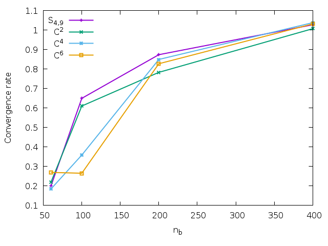
Figure 12 also shows the convergence to the analytical value of the azimuthal velocity at when both, the number of particles and neighbors rise. As stated in previous works (Zhu et al. 2015) we find that good convergence is only attained for large enough combinations of . Nevertheless, the choice of the interpolator also matters, with providing the best results on average, in the entire range of considered in this work and for any . Among the Wendlands, the interpolator is the best when , but turns to in the interval . In general, the mixed Sinc gives the best results when , and still performs well when the number of neighbors is low, , albeit slightly worse than for such low . The absolute best result among all the calculated models, , was that of both and with , (bottom right panel), significantly lower than previously reported by (Dehnen & Aly 2012) for a similar initial setting. It is similar to the best value, , obtained with the state-of-the-art relativistic SPH code by Rosswog 2015 in 2D, with the kernel, and only when coupled with the integral approach to calculating the gradients. All panels in Fig. 12 depict the line (in black) with determined with the data of the mixed Sinc interpolator. The value of steadily increases with the number of target neighbors, from at to at . This is clearly shown in Fig. 13, where we present the convergence rate as a function of the number of neighbors for different kernels. Extrapolating, it suggests that the slope could be significantly higher than provided that the number of neighbors is high enough, which is in agreement with Zhu et al. 2015. On another note, the convergence rate with , shown in the last panel of Fig. 12, is faster than that obtained in several previous calculations (Springel 2010; Dehnen & Aly 2012) and similar to the value reported by Rosswog 2015. In general terms, Fig. 13 shows that the convergence rate of the mixed Sinc kernel is higher than that of the other represented kernels and certainly higher for the range , commonly used in 3D SPH simulations.
4.3.1 Fine-tuning the mix
The results of the Gresho-Chan vortex test can be further tuned by changing the parameters in the mix, namely the Sinc exponents and the coefficient . Here we can benefit from the continuum nature of the Sinc kernels and choose among non-integer values of the exponents. Due to the many combinations, we restrict the exploration to which, according to Fig. 4, show a reasonable balance between FWHM and . A qualitative analysis can be performed in light of the adopted values of FWHM and , which we assume as the main magnitudes driving the behavior of the interpolator.
First, we choose a value of FWHM around that of our reference kernel (FWHM=1.15). Next, we vary the first exponent of the Sinc within the interval and then the second exponent, , is obtained from the FWHM by solving the inverse problem. Once the pair is known, we can determine the first zero of its FT. The results are depicted in Fig. 14 where each color corresponds to a particular value of the FWHM of the mixed kernel. We indicate the location of along the FWHM = 1.15 line with a red circle and the label 0, which serves as a reference. Next, we monitored the error of several particular points (red squares) on the lines with constant FWHM and compared them to the value obtained with . The main results are shown in Table 2, where the anticorrelation of the FWHM and the Fourier critical wavenumber is evident. We note that the deviations around the reference value are lower than . The combination with label 4 slightly enhances the results at low with minimal degradation of the others. The remaining cases follow the expected trend with better at large FWHM and low and vice versa. This suggests that previous knowledge of the number of neighbors may help to establish the optimal mix of kernel exponents. For example, combinations number 6 and 8 could be a good choice in the low- regime, but without losing too much of their pairing resistance in the high- regime.
On another note, raising the value of slightly improves the results in the high region. According to Fig. 4 the points on the line (in yellow) located at , , , and are good potential targets as they display FWHM values higher than those of and very similar values to those of (albeit slightly lower). The errors of these points are shown in Table 3 which also includes the combination, labeled as point 9 in Fig. 14 and located just above points 4 and 5. For the most part, they do not improve over the default choice except when , where there is a modest enhancement (). Figure 14 also shows the line of constant at (black solid line). Interestingly, such a line intersects with and (green solid line) at the default choice (red circle). The combination in Table 3 (point 9 in Fig. 14) slightly reduces the normalized in all cases. It could be a plausible alternative to our default .
On the same line, one may wonder if the mixing of two Wendland kernels of different orders would significantly enhance the results of the vortex test. To explore this issue, we carried out several additional simulations with the mix and compared the results with those obtained with pure Wendlands. The main results are shown in Table 4 where we can see that, for the most part, the mixing only makes small changes in the values. A comparison between , , and is shown in the last two columns of Table 4. The mixed Wendland slightly enhances the outcome of at low but the results in the high region are a bit worse. On another note, the kernel substantially improves results over the pure in the low- region but this fact is not a merit of the mix, but rather a demerit of the when . On the whole, the percent variations are similar to those shown in Tables 2 and 3 with respect to the mix of Sinc kernels.
From the experiments above we conclude that the kernel is close to the optimal choice in the interval . Nevertheless, small to moderate improvements in particular regions are possible by carefully tuning and as, for example, model 8 in Table 2 (low- enhancement) or any model in Table 3 (high- enhancement).
| Point label | 0 | 1 | 2 | 3 | 4 | 5 | 6 | 7 | 8 |
|---|---|---|---|---|---|---|---|---|---|
| (n,m) | (4.0,9.0) | (4.7,8.95) | (4.1,10.33) | (4.1,8.73) | (3.7,9.55) | (3.7,8.15) | (3.2,9.08) | (3.21,7.94) | (3.11,8.13) |
| FWHM | 1.15 | 1.10 | 1.10 | 1.15 | 1.15 | 1.20 | 1.20 | 1.25 | 1.25 |
| 1.935 | 2.037 | 1.996 | 1.946 | 1.905 | 1.884 | 1.824 | 1.813 | 1.797 | |
| 1.00 | 1.14 | 1.03 | 1.02 | 0.94 | 0.94 | 0.87 | 0.87 | 0.85 | |
| 1.00 | 0.99 | 1.05 | 0.98 | 1.02 | 0.99 | 1.03 | 1.03 | 1.04 | |
| 1.00 | 0.97 | 1.00 | 0.99 | 1.01 | 1.02 | 1.04 | 1.10 | 1.09 |
| (n,m) | (4.0,9.0) | (4.0,10.0) | (4.0,11.0) | (4.0,12.0) | (3.75,10.46) |
|---|---|---|---|---|---|
| FWHM | 1.10 | 1.10 | 1.15 | 1.15 | 1.20 |
| 1.932 | 1.946 | 1.989 | 2.421 | 1.926 | |
| 1.01 | 1.02 | 1.02 | 1.03 | 0.99 | |
| 0.94 | 0.96 | 0.98 | 1.01 | 0.98 | |
| 0.95 | 0.96 | 0.96 | 0.96 | 0.97 |
| 5.96 | 9.10 | 5.62 | 0.94 | 0.62 | ||
| 3.29 | 3.56 | 3.33 | 1.01 | 0.94 | ||
| 3.48 | 3.29 | 3.51 | 1.01 | 1.07 | ||
| 4.75 | 6.88 | 4.45 | 0.94 | 0.65 | ||
| 1.84 | 1.89 | 1.80 | 0.98 | 0.95 | ||
| 1.67 | 1.54 | 1.64 | 1.02 | 1.06 |

4.4 Shock-tube test
The numerical experiment known as the shock-tube test involves the propagation of shock and rarefaction waves in an inhomogeneous medium. In this test, a box of size is filled with a gas so that there is an initial strong contrast in density and pressure between the left and right ( regions of the box. This test has an analytical solution (Sod 1978) to compare with. Hence, we can perform the analysis of the results in light of the adopted kernel and is therefore adequate for the present study. Unlike precedent tests, the sharpness of the kernel function is relevant here if we want to resolve the shock front and the contact discontinuity. This slightly favors high-order kernels.
The onset is similar to that adopted in other works (Wadsley et al. 2017; Price et al. 2018) with , , and , in the left and right states of the box, respectively. Both regions of the 3D box are filled with particles of equal mass settled in a glass-like configuration with and particles on the left and right sides of the box, respectively. The initial density profile around the contact discontinuity was not smoothed. The large initial density and pressure jumps drive a strong shock, which makes the artificial viscosity (AV) algorithm especially relevant in this test. Previously published works (Wadsley et al. 2017) obtained good results in this test, free or almost free of velocity oscillations in the post-shock plateau, by choosing relatively high AV parameters: , in combination with AV switches (Cullen & Dehnen 2010) or with lower values, but constant, and (Price et al. 2018). In this work, we decided to use the approach by Wadsley et al. 2017 with the same choice of AV parameters.
Figure 15 shows the results of this test for kernels and , with neighbor counts of . In general, at large neighbor count exhibits slightly better results than , as expected for a higher order kernel, but the differences are not large. Furthermore, significantly outperforms at a lower neighbor count, which can be seen in the lower particle dispersion and lower values. This is consistent with the results found in previous tests, where shows a robust performance across a broad spectrum of neighbor counts.
The same behavior can be seen in Fig. 16, which shows how the error evolves with increasing number of neighbors, for the three Wendland kernels and , in the four physically relevant magnitudes. In general, both and provide low errors for a wide range of neighbor counts. On the other hand, the benefits of can only be seen when using large numbers of neighbors, and the improvement in is only marginal. The opposite is true for the Wendland which becomes competitive only at low neighbor counts, .


5 Conclusion
We reviewed the properties of the Sinc family of interpolators proposed by Cabezón et al. 2008 and extended them to consider the impact of having a binary linear mix of these kernels. Low-order Sincs have good sampling properties, but they are prone to suffering from pairing instability when the number of neighbors is high. In contrast, high-order Sincs are resistant to pairing, but suffer from bias when the number of neighbors is low33 3 Which is also true for other interpolators, such as the B-splines and Wendland kernels.. We show that an appropriate choice of the mixing coefficient considerably delays the critical wavenumber at which the Fourier transform of the kernel becomes negative, making them much more resistant to pairing instability while increasing the FWHM at the same time, which makes them less prone to bias. In this respect, the combination of low- and high-exponent Sinc functions not only produces new, spherically symmetric, and pair-resistant interpolators but also improves their internal sampling. Having good sampling properties, even when the number of neighbor particles is low or moderate, is a very desirable quality for any kernel.
The particular combination of and Sincs with mixing coefficient , namely , proved to be very suitable as an interpolator for SPH simulations. For example, it accurately reproduces the density of a homogeneous system in both, ordered lattices and glass-like particle distributions in a wide range of neighbor particles (Sect. 4.1). According to the results in Sect. 4.2, it also hinders the spawning of the pairing instability when the number of neighbors is large, . Additionally, it maintains a good partition of the unit and an accurate condition even when the number of neighbors is low, . The analysis of the results of the Gresho-Chan test in Sect. 4.3 allows us to make a detailed study of the convergence issues of the SPH scheme. This test is appropriate to contrast the quality of the results in light of the chosen kernel, either the Sinc or the widely used , , and Wendland kernels. We found that the behavior of was better on average than that of commonly used Wendland polynomials in the explored range , each with . The only exception is when the number of neighbors is very low, for which the polynomial led to the lowest values. Our results also suggest that working with , or in Eq. 5, would make the simulations less dependent on the nature of the chosen kernel and provide quite accurate results. All our results start to flatten around that value (see Figs. 8, 9, 11, and 13). Still, interpolators that can give good results even at , such as and , are valuable as they increase local resolution and reduce computational burden.
We also tested the performance of in the presence of strong shocks simulating the Sod tube in 3D. In this case, higher-order, peaked kernels are expected to be favored for properly resolving the discontinuities. Indeed, produces the lowest errors, but only for large neighbor counts and at the expense of losing spatial resolution. Wider, less peaked kernels offer a better trade-off for low and medium numbers of neighbors, making and a better choice. These results confirmed the conclusions drawn in the Gresho-Chan test, establishing as a versatile kernel, with good interpolation properties in a wide range of numbers of neighbors, and in different physical scenarios.
Summarizing, we showed that a suitable linear mix of Sinc functions, combining low and high exponents, produces new, spherically symmetric interpolators with both, better internal sampling and enhanced pair-resistant behavior. The mixed Sincs are well balanced, allowing them to work with very different initial numbers of neighbors, which can, for example, be applied in different fluid regions with the same kernel. Moreover, it makes the SPH method more robust, because the results become less sensitive to statistical fluctuations in the number of interpolating neighbor particles. Although this strategy can be used to enhance any other kernel as, for example, the popular and polynomials, it is well suited to the Sincs because of their continuum nature, which endows them with great flexibility. According to Fig.4 it is enough to carefully choose the exponents () and the mixing coefficient so that particle clustering is avoided once the initial number of neighbors has been chosen. Incorporating such a mixture of kernels into an SPH code is straightforward and encompasses little overall difference in computational burden. This is because the mixed interpolator and its gradient can be tabulated and loaded at the beginning of the calculation. It makes therefore feasible to work with non-integer Sinc exponents to fine-tune the results, as shown in Sect. 4.3.1.
Although the results of this work point to a very positive impact of combining kernels of a different order, work has to be done to extend the analysis to different physical situations than those considered in this work, for example, instability growth and turbulence simulation. A robust interpolator, capable of coping with both, low and high numbers of neighbor particles, may help to balance the resolution among fluid regions with very different densities without the need of having particles with different masses. This is an interesting line of development that will make the SPH technique even more adaptive.
Acknowledgements
This work has been supported by the MINECO Spanish project PID2020-117252GB-100 grant SGR-386/2021, by the AGAUR/Generalitat de Catalunya (DG) and by the Swiss Platform for Advanced Scientific Computing (PASC) project SPH-EXA2: Smoothed Particle Hydrodynamics at Exascale (RC). The authors acknowledge the support of the center for scientific computing: sciCORE (http://scicore.unibas.ch) at the University of Basel, where part of these calculations was performed.
Data Availability
Data supporting this article will be shared on reasonable request with the corresponding author. A current version of SPHYNX is publicly available at: https://astro.physik.unibas.ch/sphynx
References
- Arth et al. (2019) Arth A., Donnert J., Steinwandel U., Böss L., Halbesma T., Pütz M., Hubber D., Dolag K., 2019, arXiv e-prints,
- Cabezón et al. (2008) Cabezón R. M., García-Senz D., Relaño A., 2008, Journal of Computational Physics, 227, 8523
- Cabezón et al. (2017) Cabezón R. M., García-Senz D., Figueira J., 2017, A&A, 606, A78
- Cullen & Dehnen (2010) Cullen L., Dehnen W., 2010, MNRAS, 408, 669
- Dehnen & Aly (2012) Dehnen W., Aly H., 2012, MNRAS, 425, 1068
- Dilts (1999) Dilts G. A., 1999, International Journal for Numerical Methods in Engineering, 44, 1115
- Fulk & Quinn (1996) Fulk D. A., Quinn D. W., 1996, Journal of Computational Physics, 126, 165
- García-Senz et al. (2012) García-Senz D., Cabezón R. M., Escartín J. A., 2012, A&A, 538, A9
- García-Senz et al. (2014) García-Senz D., Cabezón R. M., Escartín J. A., Ebinger K., 2014, A&A, 570, A14
- García-Senz et al. (2022) García-Senz D., Cabezón R. M., Escartín J. A., 2022, A&A, 659, A175
- Gingold & Monaghan (1977) Gingold R. A., Monaghan J. J., 1977, MNRAS, 181, 375
- Gresho & Chan (1990) Gresho P. M., Chan S. T., 1990, International Journal for Numerical Methods in Fluids, 11, 621
- Hu et al. (2014) Hu C.-Y., Naab T., Walch S., Moster B. P., Oser L., 2014, MNRAS, 443, 1173
- Lucy (1977) Lucy L. B., 1977, AJ, 82, 1013
- Monaghan (1992) Monaghan J. J., 1992, ARA&A, 30, 543
- Monaghan (2005) Monaghan J. J., 2005, Reports on Progress in Physics, 68, 1703
- Price (2012) Price D. J., 2012, Journal of Computational Physics, 231, 759
- Price et al. (2018) Price D. J., et al., 2018, Publ. Astron. Soc. Australia, 35, e031
- Read & Hayfield (2012) Read J. I., Hayfield T., 2012, MNRAS, 422, 3037
- Rosswog (2015) Rosswog S., 2015, MNRAS, 448, 3628
- Rosswog et al. (2023) Rosswog S., Torsello F., Diener P., 2023, arXiv e-prints, p. arXiv:2306.06226
- Schuessler & Schmitt (1981) Schuessler I., Schmitt D., 1981, A&A, 97, 373
- Sod (1978) Sod G. A., 1978, Journal of Computational Physics, 27, 1
- Springel (2010) Springel V., 2010, ARA&A, 48, 391
- Springel & Hernquist (2002) Springel V., Hernquist L., 2002, MNRAS, 333, 649
- Valdarnini (2016) Valdarnini R., 2016, ApJ, 831, 103
- Wadsley et al. (2017) Wadsley J. W., Keller B. W., Quinn T. R., 2017, MNRAS, 471, 2357
- Wendland (1995) Wendland H., 1995, Advances in Computational Mathematics, 4, 389
- Zhu et al. (2015) Zhu Q., Hernquist L., Li Y., 2015, ApJ, 800, 6