Reciprocity and sensitivity kernels for sea level fingerprints– \eqsecnum
Reciprocity and sensitivity kernels for sea level fingerprintsVolume: 142
keywords
Reciprocity theorems are established for the elastic sea level fingerprint problem including rotational feedbacks. In their simplest form, these results show that the sea level change at a location due to melting a unit point mass of ice at is equal to the sea level change at due to melting a unit point mass of ice at . This identity holds irrespective of the shoreline geometry or of lateral variations in elastic Earth structure. Using the reciprocity theorems, sensitivity kernels for sea level and related observables with respect to the ice load can be readily derived. It is notable that calculation of the sensitivity kernels is possible using standard fingerprint codes, though for some types of observable a slight generalisation to the fingerprint problem must be considered. These results are of use within coastal hazard assessment and have a range of potential applications within studies of modern-day sea level change.
1 Introduction
[21] provided the first gravitationally self-consistent theory of post-glacial sea level change on a non-rotating, 1-D (depth varying) viscoelastic Earth for the case of time-invariant shoreline geometry. Their static “sea level equation” has played a central role in the modern development of the field of glacial isostatic adjustment (GIA) and, in the intervening half century, their theoretical treatment has been extended to incorporate 3-D viscoelastic Earth structure and to include both rotational effects on sea level and shoreline migration due either to local sea level fluctuations or changes in the perimeter of grounded, marine-based ice (Mitrovica & Milne 2003; Kendall et al. 2005).
The predictions appearing in Farrell & Clark 1976 included the special case of elastic Earth models (e.g., their Figs. 3,4), appropriate for considering the sea level response to ice mass flux with a time scale shorter than the viscous relaxation time. The calculations highlighted the counter-intuitive result that sea level falls in the vicinity of a rapidly melting ice sheet due to the combined effects of elastic crustal uplift and the loss of gravitational attraction towards the diminishing ice cover. The maximum sea level fall adjacent to the ice sheet is an order of magnitude (or more) greater than the global mean sea level (GMSL) rise associated with the melt event, while at large distances from the ice sheet the predicted sea level rise is up to % greater than GMSL.
Clark & Lingle 1977 and later Clark & Primus 1987 highlighted the relevance of the elastic case for predicting geographically variable sea level change arising from ice sheet mass flux driven by modern global warming. The latter was cited by Mercer 1978 in his canonical study of the vulnerability of the West Antarctic Ice Sheet to climate change and the implications of its potential collapse for the Earth system. The connection was further reinforced by Conrad & Hager 1997 who quantified the potential bias in estimates of GMSL based on the existing distribution of tide gauge records. Mitrovica et al. 2001 were the first to demonstrate that geographic variability in a subset of tide-gauge determined sea level rates could be reconciled by specific combinations of melt sources. Their predictions included rotational effects and they emphasised the unique geometry, or fingerprints (Plag & Juettner 2001), of sea level change associated with each ice sheet or glacier. The notion of “fingerprinting” the individual sources of melt-water has subsequently become a central theme in the analysis of modern sea level observations (Tamisiea et al. 2001; Milne et al. 2009; Plag 2006; Bamber & Riva 2010; Mitrovica et al. 2011; Brunnabend et al. 2015; Spada & Galassi 2016, e.g.). Moreover, the inclusion of fingerprint physics in such analysis has led to a significant revision in estimates of 20th century GMSL (Hay et al. 2015; Dangendorf et al. 2017).
In all the above analyses, sea level fingerprints were predicted for specific, assumed geometries of ice mass flux and this has hindered the adoption of such models in assessments of coastal hazards posed by a warming world. Three recent studies have inverted these analyses by developing methods for producing a map that shows the variation in sensitivity of sea level at a specific site to ice mass changes anywhere within the cryosphere (Larour et al. 2017; Mitrovica et al. 2018; Crawford et al. 2018). These maps represent sensitivity kernels that can be integrated with arbitrary ice mass flux geometries to compute the sea level changes at any site of interest. The Larour et al. 2017 approach was based on an automatic differentiation tool applied to sea level software that solved the forward problem (i.e., computation of the sea level fingerprint associated with a specific ice mass flux), while Mitrovica et al. (2018) solved a large number of forward problems in which a grid-by-grid perturbation in ice thickness was prescribed and applied a finite-difference approximation. Lastly, Crawford et al. 2018 applied the adjoint method to the equations governing the full sea level problem within a viscoelastic earth model, obtaining results for elastic fingerprints as a special case. An advantage of this latter method is that it yields exact sensitivity kernels at a cost equivalent to just two forward calculations (and just one in the case of the fingerprint problem). A limitation of that study, along with earlier work on adjoint methods for GIA (Al-Attar & Tromp 2014; Martinec et al. 2015), was the neglect of rotational feedbacks. Moreover, the results of Crawford et al. 2018 that are relevant specifically to fingerprints are embedded within the more complex viscoelastic theory which makes them harder to understand and apply.
In this article we revisit the derivation of sensitivity kernels through a different and simpler argument that is specialised to the elastic fingerprint problem with rotational feedbacks included and with a fixed shoreline geometry. The latter assumption renders the fingerprint problem linear and is appropriate within applications to modern sea level where amplitudes of change are low. Our presentation is deliberately independent of Crawford et al. 2018, and hence a knowledge of that work and the Lagrange multiplier methods on which it is based is not necessary to understand this paper. We proceed here by first establishing reciprocity theorems for the fingerprint problem along with suitable generalisations thereof. In their simplest form, these results show the following: Suppose that at some location, , a unit point mass of ice is melted and the sea level change is observed at . This sea level change is identical to that that would be observed at due to melting a unit point mass of ice at . The derivation makes no assumptions about the shoreline geometry nor internal structure of the earth model, and hence this is not merely a geometric symmetry of the problem. With the reciprocity theorems at hand, it is a simple matter to obtain sensitivity kernels for the whole range of physically relevant observables. In the case of observables depending directly on sea level change (e.g. tide gauge determined rates), calculation of the sensitivity kernel can be performed using a standard fingerprint code. When more general observables are considered (e.g., those associated with satellite altimetry or gravity) a generalised form of the fingerprint problem must be solved, but the necessary changes are slight. While the focus of this work is on sea level change driven by the growth or melting of continental ice sheets, it is worth commenting that the theory developed is applicable to other types of surface loading such as that associated with hydrology, ocean dynamics or sedimentation.
2 Sensitivity kernels in non-rotating earth models
Within this section we derive reciprocity theorems for the elastic fingerprint problem in a non-rotating earth model and show how they can be used to obtain sensitivity kernels for sea level (and other observables) with respect to ice thickness. The necessary extensions to account for rotational feedbacks are described in Section 3. Splitting the theory in this manner is unnecessary but we think it helpful to incrementally add complicating factors into the problem.
2.1 Equations of motion for static loading
We start by considering the static loading of a non-rotating elastic earth model. The volume of the earth model will be written and its surface . It is assumed that, prior to application of the load, the earth model is in a state of hydrostatic equilibrium, with its gravitational potential written . As discussed in Section 2.3.2 of Al-Attar & Tromp 2014, the response of such a model to a surface load, , is governed by the following equations of motion expressed in the weak form
| (1) |
Here is the displacement vector, the Eulerian gravitational potential perturbation, while and are corresponding test functions. We recall that within the weak formulation, the fields solve the problem if the above equation holds for arbitrary test functions (subject to standard regularity conditions). The term , which is associated with the elastic and gravitational response of the earth model, is a bilinear form whose definition can be found in eq.(2.52) of Al-Attar & Tromp 2014. For our purposes, we need only the following two properties of this bilinear form:
- 1.
It is symmetric in the sense that
(2) Note that within the identity the displacement and gravitational potential perturbations are paired together; we cannot, for example, interchange the two displacements vectors alone.
- 2.
For any test functions , the following identity holds
(3) when the displacement and gravitational potential perturbation take the form
(4) with arbitrary constant vectors and . The fields and defined here correspond to a linearised rigid body motion, with the vector parameterising the translational degrees of freedom and those of rotation.
Using these two properties, we can take
| (5) |
within eq.(1) to arrive at a trivial equality. From this it follows via the Fredholm alternative (e.g Marsden & Hughes 1983, Chapter 6) that the static loading problem admits a solution for any , but that the solution is only defined up to a linearised rigid body motion (c.f. Martinec et al. 2015, Section 3).
2.2 A first reciprocity theorem
Suppose that solve the static loading problem for a load , and that solve the static loading problem for some other load . From eq.(1), we know that
| (6) |
In exactly the same way for the second problem, we can write
| (7) |
Subtracting one equality from the other and using the symmetry of , we arrive at the non-trivial identity
| (8) |
This is not a new result. It was obtained by Tromp & Mitrovica 1999 within the context of quasi-static loading problems and is, as they pointed out, a generalisation of Betti’s reciprocity theorem that is well-known in seismology (Aki & Richards 2002, e.g.).
2.3 Reformulating the theorem in terms of sea level
Within gravitationally self-consistent sea level theory (Farrell & Clark 1976; Mitrovica & Milne 2003; Crawford et al. 2018, e.g.), deformation of the earth model can be related to sea level change, , through the relation
| (9) |
where is the magnitude of gravitational acceleration at the surface. Here we note that we are working with a hydrostatic theory in which sea level is defined as difference been the equipotential that defines the sea surface and the solid surface (Mitrovica & Milne 2003; Tamisiea 2011, e.g.). The first term on the right hand side of eq.(9) is associated with vertical motion of the solid surface, the second with changes in the shape of equipotential surfaces, while the spatially constant final term, , is linked to variations in ocean mass. As a comment on notations, within this paper, we consider sea level change, , along with related quantities such as ice thickness change, or global mean sea level change that are defined later. Because, however, all equations are linear and have no explicit time-dependence, we could equally well have chosen to work with with rates of change of these quantities. The value of the constant is fixed by conserving mass between the oceans and direct load, with this requirement conveniently written as
| (10) |
Here the total load, , is decomposed into an ocean load and a direct load, , as
| (11) |
where is the density of water and the ocean function that equals one where water is present and zero otherwise. In the case of ice loading, the direct term is given by
| (12) |
where is the density of ice, and the change in ice thickness. The factor, , within this expression accounts for the possibility of floating ice (e.g. Crawford et al. 2018, equations 31–34).
Consider again a pair of solutions and of the loading problem associated, respectively, to with loads and . Here, however, we assume that these loads are decomposed as in eq.(11) into water and direct terms that share a common ocean function. From the above expression for sea level change we can write
| (13) |
and hence eq.(8) becomes
| (14) |
The terms involving the constants and vanish due to conservation of mass, and so the identity simplifies to
| (15) |
If we now substitute into the equality the decompositions of the loads, and , we find
| (16) |
and cancelling the terms symmetric in and we arrive at
| (17) |
Again, this is a known result, being implied as a special case by the adjoint theory of Crawford et al. 2018 for sea level change in a viscoelastic earth model. What is new is the explicit statement as a reciprocity theorem along with the more elementary derivation that has been facilitated by restricting attention to the elastic fingerprint problem.
2.4 Symmetry of the Green’s function
Because the fingerprint problem is linear, its solution must take the form
| (18) |
for an appropriate Green’s function, where we have added a subscript to the surface element to make clear which variable it is defined with respect to. Suppose that, within eq.(17), we take
| (19) |
with being the delta function on based at which is defined such that
| (20) |
for any suitably regular function, . By definition of the Green’s function, it follows that , and hence from the reciprocity theorem we arrive at the identity
| (21) |
Such a symmetry of the Green’s function was established for static loading problems by Tromp & Mitrovica 1999 in cases where there is only a direct load. Here we see the result remains true when a gravitationally self-consistent water load is included. It is this symmetry that makes precise our earlier statements of the reciprocity theorem in terms of the response to melting unit point masses of ice.
2.5 Self-adjointness of the sea level equation
An alternative description of the sea level reciprocity theorem can be given in the language of functional analysis. Solution of the the sea level equation implicitly defines a linear mapping, , from the direct load, , to the resulting sea level change, , with both scalar fields being defined on the surface, , of the earth model. Using this notation within eq.(17), we have
| (22) |
Regarding the integral, , of two real-valued scalar fields, and , on as an inner product, it follows that the operator, , is self-adjoint (Schechter 2001, e.g.). To make these ideas precise, one should specify the domain and range of the operator, . We will not dwell on such technical points nor pursue this operator formalism further within this work, but note that these ideas can also be applied to the generalised reciprocity theorems discussed below.
2.6 Sensitivity kernels for sea level change
Suppose now that is some functional of the sea level change. For example, within the context of an inverse problem to recover the direct load we might consider
| (23) |
where is the observed sea level change and the ocean function is included to limit contributions to the oceans. Because is obtained by solving the sea level problem for a given direct load, , this functional implicitly depends on . It can, for a variety of reasons, be interesting to determine the functional derivative of with respect to . To do so, we write for the perturbation in the direct load, and for the corresponding perturbation to . Working to first-order in perturbed quantities, we have
| (24) |
for the above example, or more generally
| (25) |
for some appropriate determined by the choice of . Because the fingerprint problem is linear, eq.(17) immediately holds with replaced by , and hence the reciprocity theorem then gives
| (26) |
where is obtained by solving the fingerprint problem subject to the direct load . This shows that is the sensitivity kernel of with respect to . Recalling that in the case of an ice load we have , it follows that we can equivalently write
| (27) |
from which we can identify the sensitivity kernel of with respect to the ice thickness
| (28) |
These results are special cases of those obtained by Crawford et al. 2018. Following the terminology of that work, we will call the adjoint sea level and the adjoint load. What this new derivation makes clear is that sensitivity kernels can be obtained by solving the standard fingerprint problem subject to an appropriate adjoint load.
2.7 Dealing with more complex observables
We have now seen that sensitivity kernels can be readily obtained for functionals, , defined in terms of the sea level change, . In practice there are, of course, other quantities that can be observed, including changes in sea surface height or in the gravitational potential. To obtain analogous results for such observables, it is necessary to consider the generalised loading problem
| (29) |
where we have introduced additional forcing terms and . These terms need not have a direct physical interpretation, but we will see that the term allows us to consider functionals depending directly on the surface displacement, while is needed for those involving the gravitational potential perturbation. Recalling the second property of the bilinear form mentioned above, it follows that a necessary and sufficient condition for solutions to exist is
| (30) |
with and arbitrary constant vectors. The practical significance of this condition will be explained below.
A reciprocity theorem for the generalised loading problem can be obtained as before by introducing pairs of solutions and corresponding, respectively, to the generalised loads and . The result is the following identity
| (31) |
By decomposing the loads and into direct terms and matching water loads, the above identity becomes
| (32) |
which is a reciprocity theorem for the generalised fingerprint problem.
Suppose that we define some functional in terms of the solution to the fingerprint problem and wish to determine its functional derivative with respect to the direct load, . To first-order, the perturbation in can be written
| (33) |
for suitable choices of . Eq.(32) then leads immediately to the desired relation
| (34) |
with the adjoint sea level, obtained through the solution of the generalised fingerprint problem subject to the generalised loads defined within eq.(33). Here we must ask whether the problem for has a well-defined solution, this requiring
| (35) |
for any constant vectors and . Clearly, however, this condition is equivalent to the requirement that the value of is invariant under linearised rigid body motions. Equally, the solution to the generalised fingerprint problem is only defined up to a linearised rigid body motion, but such a term makes no contribution to the resulting sea level change, . The end result is that the sensitivity kernels are well-defined so long as we work with observables that are physically meaningful.
3 Sensitivity kernels in rotating earth models
Having established the basic methods in a non-rotating earth model, we show in this section how rotational feedbacks can be incorporated into the problem. Doing this requires a brief review of rotational dynamics for a deforming planet, but once this is done we can proceed very quickly to the final results.
3.1 Review of some rotational dynamics
Consider an earth model rotating steadily with angular velocity, . The steady-state Euler equation takes the form
| (36) |
where is the inertia tensor. As is well-known, this equation requires that be along a principle axis of , and we assume that this is the axis having the largest moment of inertia, . Suppose that the earth model is deformed such that its inertia tensor is perturbed to . The steady-state rotation vector will be perturbed to , and from the Euler equation we obtain to, first-order accuracy,
| (37) |
where for convenience we have set . Taking the cross product with and using standard vector identities, we find that
| (38) |
where the subscript ⟂ is used to denote projections orthogonal to the reference rotation axes; note that when restricted to such vectors the matrix is non-singular. To fix the component of along the rotation axes, we note that conservation of angular momentum requires
| (39) |
which to first-order yields
| (40) |
where the subscript ∥ is used to denote projections parallel to the reference rotation axes. These results can be summarised by saying that
| (41) |
with a symmetric and invertible matrix. Relative to a Cartesian basis aligned with the principle axes of , we note that
| (42) |
where are the principle moments of inertia. Because , it is common to neglect the component of along the -axis. This approximation will be made within our numerical calculations, but the reciprocity relations derived below hold whether or not this is done.
Associated with the equilibrium rotation vector we can define the centrifugal potential
| (43) |
and hence the first-order perturbation, , to this potential is given by
| (44) |
The negative gradient of the centrifugal potential gives the centrifugal acceleration that is needed within the equations of motion, and so we note the following relations:
| (45) |
We now need to relate an applied surface load and associated deformation of the earth model to the perturbed inertia tensor, . As a starting point, we note that the earth model’s equilibrium inertia tensor satisfies the identity
| (46) |
with the equilibrium density, and where here is an arbitrary vector. When subject to a surface load, , the first-order perturbation in this quantity can be written
| (47) |
where standard vector identities have been applied. Here, the first term is due to internal deformation and the second is the direct contribution of the load. Changing within this identity to and expanding to first-order in we obtain
| (48) |
where we recall that . Comparing the two integrands with the expression for and obtained above, we arrive at an identity that will be useful later
| (49) |
Within this equality it should be emphasised that is the centrifugal potential perturbation associated with , while is the inertia perturbation associated with the applied load, , and the associated displacement, .
The derivations within this section have assumed that the earth model is entirely solid. As shown by Dahlen 1974, in considering the static deformation of an earth model with a fluid (outer) core, the linearised Lagrangian displacement vector is not well-defined in fluid regions. Instead, Dahlen showed that an Eulerian formulation within fluid regions could be applied, with all relevant variables then expressed in terms of the perturbed gravitational potential. The necessary extensions of our arguments to earth models containing fluid regions are simple but will not be given because the form of the reciprocity theorems is unchanged.
It is also worth commenting that, when calculations are performed in a spherically symmetric earth model, the reference inertia tensor, , is taken to be that observed for the Earth (Mitrovica et al. 2005; Mitrovica & Wahr 2011, c.f.). Here, there is an assumption that the deformation of the Earth due to the applied load can be sufficiently well-approximated by the response of a spherical earth model. Again, the reciprocity theorems hold whether or not this approximation is made.
3.2 Reciprocity theorems including rotational feedbacks
We start with the equations for a static loading problem in a rotating earth model in weak form,
| (50) |
Here, is the centrifugal potential associated with the perturbed rotation vector, , and we see that this term is associated with a tidal force applied to the earth model (c.f. Bagheri et al. 2019, Appendix B). Note also that a new test function, , has been added to enforce the relation between and the inertia tensor perturbation in eq.(41), the latter term depending implicitly on and the applied load, . Following a now familiar procedure, we let be the solution of the problem subject to a load , and use this to obtain the identity
| (51) |
where we note that terms involving the matrix have vanished due to its symmetry. Using eq.(49) twice, this simplifies to
| (52) |
This is a new result which extends the reciprocity theorem of Tromp & Mitrovica 1999 to incorporate rotational feedbacks.
To express eq.(52) in terms of sea level change, we need merely note that, once rotational feedbacks are present, the relation between sea level change, , and surface deformation is generalised to
| (53) |
which follows due to the sea surface now lying on an equipotential of the combined gravitational and centrifugal potentials. Given this relation, our earlier argument proceeds identically to give
| (54) |
which takes the same form as in the non-rotating case in eq.(17). From this identity we can readily show the symmetry of the Green’s function and obtain sensitivity kernels for any functional of the sea level change. These results are new, extending the work of Crawford et al. 2018 to include rotational feedbacks in the case of elastic fingerprint problems. Extensions of the general viscoelastic adjoint theory to incorporate rotational feedbacks can be carried out along similar lines, but the results will be presented elsewhere.
Finally, if we wish to consider observables other than sea level, it is necessary to consider the generalised loading problem
| (55) |
where an additional force term, , has been included to facilitate observations depending directly on . Here, we must account for the contribution of the direct gravitational load, , to the perturbed inertia tensor, this leading to eq.(49) being generalised to
| (56) |
Following the now standard argument, we arrive at the reciprocity theorem
| (57) |
To remove the explicit dependence on the centrifugal potentials, we note from eq.(44) that and hence
| (58) |
which is an alternative form that can sometimes be useful.
4 Numerical verification and initial applications


Within this final section, we describe a range of numerical calculations that (i) provide a check on the correctness our theoretical results and (ii) illustrate the potential of these methods within future practical applications. All these calculations are done using a spherically symmetric earth model, but we note that the general theory is applicable within laterally varying elastic earth models. The use of spherically symmetric earth models is common within fingerprint calculations and it has been shown by Mitrovica et al. 2011 that lateral variations in elastic structure have only a minor effect in this context.
4.1 Summary of the numerical method
To solve the elastic fingerprint problem, we apply the standard pseudo-spectral method (Mitrovica & Peltier 1991) with rotational feedbacks incorporated following Milne & Mitrovica 1996; Milne & Mitrovica 1998. Fast spherical harmonic transformations are performed using the SHTOOLS library of Wieczorek & Meschede 2018. Within all calculations, a truncation degree of is used, but it has been verified that truncation at a higher degree does not appreciably change any of the results.
To account for deformation of the solid earth, we use loading and tidal Love numbers (Love 1911). For example, for a surface load, , that has spherical harmonic decomposition
| (59) |
the resulting surface vertical displacement, , and gravitational potential, , have coefficients
| (60) |
with and the loading Love numbers (as defined in this work). Here denotes an orthonormalised real spherical harmonic of degree and order defined following Wieczorek & Meschede 2018 (note that the definition used for these functions does not include the Condon-Shortley phase).
The generalised fingerprint problem involves additional like-load terms, and , introduced within eq.(29). Within the following examples, we limit attention to functionals whose dependence on the surface displacement is only through the vertical component. It is, therefore, sufficient to assume
| (61) |
for a scalar-valued function . We can then proceed by introducing suitably generalised loading Love numbers. If and are spherical harmonic expansion coefficients of and , the associated coefficients for and can be written
| (62) |
where , , , and are the generalised loading Love numbers. Calculation of these Love numbers proceeds in the same manner as the usual, with the only difference being the form of the forces applied when solving the elastostatic equations. From these definitions we note the relations
| (63) |
while, by applying eq.(31), we also have
| (64) |
which provides a useful check within numerical calculations. Values for these generalised loading Love numbers along with the usual tidal Love numbers have been calculated for PREM (Dziewonski & Anderson 1981) up to degree 4096 using the radial spectral element method of Al-Attar & Tromp 2014. Translational non-uniqueness within the degree-one problem is removed by requiring that the combined centre of mass of the earth model and surface loads is fixed. The remaining rotational degrees of freedom do not affect the observables we consider, and hence they can be ignored.
4.2 Generating a synthetic data set
Within Fig.1 we summarise the synthetic data set used in later examples. For the purposes of this paper, the specific change in ice thickness that has been chosen is arbitrary, but for definiteness it was constructed as follows. Within the northern and southern hemispheres the changes in ice thickness were separately set to be constant fractions of the present-day ice thickness within ICE6G (Argus et al. 2012; Peltier et al. 2015). These two contributions were then linearly combined such that % of the ice mass loss was sourced from the northern hemisphere, while the overall magnitude was fixed by requiring the global mean sea level change equal mm. Using this change in ice thickness, , as an input, the sea level equation was solved to obtain the resulting sea level change, , vertical displacement, , gravitational potential perturbation, , rotation vector, , and centrifugal potential perturbation, , with Fig.1 also showing the first three of these outputs.
4.3 Sensitivity kernels for point measurements of sea level


As noted previously, the sensitivity kernel for a point measurement of sea level at a location can be obtained taking the adjoint load, , to be a delta function at the observation point. Within Fig.2 we show the results of such a calculation for Boston, Massachusetts. Within sub-figure (a), the sensitivity kernel, , for this measurement with respect to the direct load, , is plotted. As might be expected, this sensitivity is greatest at the observation point and falls in magnitude rapidly away from it. The value of the kernel at the observation point is positive. This means that an increase of the direct load in the vicinity of Boston would be associated with a local rise in sea level. Such behaviour is, of course, consistent with the known physics of sea level change.
To check quantitatively whether this kernel is correct, we can numerically evaluate and compare either side of eq.(54) using the load and sea level shown in Fig.1. For the left hand side of the identity, we evaluate numerically using the solution, , of the adjoint problem along with the direct load, , applied within the forward problem. The right hand side of the identity is given by , and this can be determined by numerical integration or simply through evaluation of at the observation point. The relative difference between the values obtained was of order which is about the accuracy of the numerical calculations (no formal error analysis of the numerical methods has been undertaken). This test has been repeated using a range of different direct loads, while similar comparisons have been made for each the kernels corresponding to each of the observables discussed below.
The sensitivity kernel of sea level with respect to ice thickness is given by which is plotted in Fig.2 (b) for the Boston measurement. Here it is worth noting that this kernel can be non-zero anywhere on land. It makes sense, however, in most applications to multiply this kernel by a function that equals one in glaciated regions and by zero elsewhere. This has been done in Fig.1 (c), and now we are able to see more interesting spatial variability. This kernel does, however, contain some high-wavenumber oscillations, with this feature being more pronounced when lower truncation degrees are used within the calculations. The reason is that a delta function cannot be accurately represented using truncated spherical harmonic expansions (nor in any finite-dimensional basis). For some applications these oscillations have no practical effect and can be ignored. However, a simple and pragmatic way to remove the oscillations is to replace the point load by an appropriate smooth averaging function (c.f. Al-Attar & Tromp 2014, Appendix E). The resulting kernel is shown in Fig.1 (d) obtained using an averaging function with a characteristic length-scale of one degree (in more detail, the Green’s function for the heat equation on a sphere was used, with the time chosen such that diffusion over the desired length-scale has occurred). The result of this latter calculation can be compared with Fig.1 in Mitrovica et al. 2018 which shows a sensitivity kernel for sea level at Boston (along with several other locations) to variations in ice thickness over Greenland. Within that paper, a finite-difference approach was used to obtain these sensitivity kernels, and this required many forward calculations. Using our present methods such kernels can be determined for any desired location through a single fingerprint calculation.
4.4 Sensitivity kernels for vertical displacement measurements


Consider a measurement of vertical displacement at a surface location , made using the Global Positioning System (GPS) (Khan et al. 2010, e.g.). We can determine the sensitivity kernel for such a measurement with respect to the direct load by solving the generalised fingerprint problem subject to the following adjoint loads:
| (65) |
The result of two such calculations is shown in Fig.3 for SENU station in Greenland and DUPT in Antarctica. Here, as before, we have used smoothed point loads to remove non-physical oscillations from the kernel. It should be emphasised that in these examples, the displacements are computed relative to the combined centre of mass of earth model and surface loads. A translation of these results to any other reference system (e.g., the centre of mass of the solid Earth) is straightforward. The aim of these examples is merely to show that the calculation of such sensitivity kernels can be readily done, with the practical application of these ideas to be discussed in future work.
4.5 Sensitivity kernels for gravitational potential coefficients


We consider the measurement of a spherical harmonic coefficient of the gravitational potential at degree as might be obtained using GRACE or GRACE-FO (Tapley et al. 2004; Landerer et al. 2020, e.g). For definiteness, we use real, fully-normalised spherical harmonics, denoting the th function by . In determining the adjoint loads for this application, we use eq.(3.2) to select a value for such that the dependence on is removed from the right hand side, with this result:
| (66) |
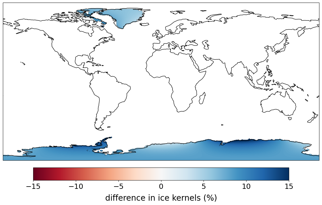
Example sensitivity kernels for and are shown in Fig.4. The kernel with respect to is plotted globally in (a), while that for ice thickness is projected onto glaciated regions in (b).


The kernels just shown reflect contributions to the potential coefficient associated with both the direct load and the gravitationally self-consistent water load it must induce. They can be usefully contrasted with kernels that account only for the direct load. In the latter case we can simply write
| (67) |
with the loading Love number for at degree . Given this relation, we then have
| (68) |
with the radius of the earth model, and hence we conclude that the relevant kernel is . In Fig.4 (c), we show the relative difference between the sensitivity kernel with respect to the direct load in (a) and the simpler kernel just defined. As might be expected, the relative differences are largest within the oceans, but even on land they can be of the order of several percent. Finally, in (d) we plot the corresponding difference between the ice kernels over glaciated regions, observing that its magnitude can in places be upwards of ten percent. Within Fig.5 we show the same thing for a higher-degree coefficient of the gravitational potential, specifically and . Here, we see smaller differences due to the neglect of induced water loads, but again the differences are most significant within the oceans. These results are consistent with the work of Sterenborg et al. 2013 who showed that methods for analysing GRACE or GRACE-FO data that do not account for induced water loads suffer from systematic biases. Within the present examples we see, in particular, that the importance of the induced water load is scale-dependent, decreasing as the dominant wave-number of the direct load increases.


Building on the previous example, we now consider the use of GRACE coefficients to estimate surface mass changes within ice sheets (Velicogna & Wahr 2006, e.g.) following the widely used method of Wahr et al. 1998 and Swenson & Wahr 2002. In the notations of this present paper, the approach starts with relation
| (69) |
between the spherical harmonic coefficients of the surface load and those of the resulting gravitational potential perturbation. Here, by use of the appropriate loading Love number, we are accounting for the direct gravitational effect of the surface mass along with the contribution to associated with deformation of the earth model (c.f. Wahr et al. 1998, eq.(12)). We assume that the potential coefficients at degrees zero and one vanish, the former due to conservation of mass and latter because the measurements are made relative to the centre of mass frame. For , the Love numbers are non-zero and so we can write
| (70) |
and hence we can reconstruct the load through
| (71) |
where an approximately equals sign is included because terms for are excluded. Errors in GRACE observations are known to increase quite rapidly as a function of degree (e.g. Swenson & Wahr 2002, Figure 1), and so the summation in eq.(71) must be truncated at some finite-degree, , with the the choice being common. Using this approach one can obtain point-estimates of surface loads from GRACE data. In fact, it is often more useful to estimate average loads over a specific region of interest. This is done by introducing an averaging function, , and then using eq.(71) to obtain
| (72) |
with the expansion coefficients of the averaging function; in what follows, we call the right hand side of this expression the “GRACE estimate” of the load. The design of optimal averaging functions for a region has been discussed by Swenson & Wahr 2002, but in our numerical examples we only use the simple Gaussian functions of Wahr et al. 1998.
From eq.(72), we can equivalently write the GRACE estimate as
| (73) |
where we have defined
| (74) |
with, again, the summation leaving implicit the inclusion of only degrees . In this manner, we can apply the reciprocity theorem stated in eq.(3.2) to write
| (75) |
where is obtained by solving the generalised fingerprint problem subject to the adjoint loads
| (76) |
The sensitivity kernel, , in eq.(75) quantifies the manner in which the GRACE estimate depends on the direct load. Within regions covered by grounded ice, the direct load and the total load, , are equal and hence the difference between and determines the accuracy of the GRACE estimate. For example, if the equality were to hold exactly then
| (77) |
and hence, in the absence of observational errors, the GRACE estimate would provide the exact average of the direct load over the chosen region. Differences between and are, therefore, indicative of systematic biases within the GRACE estimate due to the neglect of indirect water loading.
To illustrate these ideas, we show in Fig.6 (a) such an averaging function targeted at West Antarctica. Specifically, we have used a Gaussian function as defined as in eq.(32) of Wahr et al. 1998, with its centre at ( S, W), and with a half-width of km. A value of m as an equivalent water thickness was determined for the GRACE estimate from our synthetic data set assuming a truncation-degree of . This compares to the true value of m, meaning a relative error of % associated with the method. To understand this difference, we show in Fig.6 (b) the sensitivity kernel with respect to direct load for the estimate and in (c) the relative difference between this kernel and the averaging function (with values normalised relative to the maximum value of the latter field). While the relative difference between and is everywhere below about %, this difference is non-zero over much of the Earth’s surface, and it is this feature that accounts for the comparatively large error in the GRACE estimate. Analogous calculations are shown in Fig.7 for an averaging function targeted on the Greenland ice sheet; in detail the function is centred on ( N, W) and has a half-width of km. In this case, the relative error in the GRACE estimate was found to be % which is, again, significantly larger than the point-wise difference between the averaging function and associated sensitivity kernel. The forward-modelling results discussed here are consistent with those of Sterenborg et al. 2013, but what is new is the use of sensitivity kernels to quantify more fully the source of the bias.
A point worth considering is that, while GRACE does not provide coefficients for , the averaging function for the region of interest will usually have some power at these degrees. It has been shown (Chambers et al. 2007, e.g.) that this can lead to significant biases within the load estimates, while efforts to constrain the missing coefficients have been discussed using additional information and assumptions (Chambers et al. 2004; Swenson et al. 2008). It might, therefore, be reasonably asked if the errors seen within our GRACE estimates are due predominantly to missing data at degrees . If this were true, then the plots of shown in sub-figure (c) of Fig.6 and Fig.7 should closely approximate where denotes the projection of the averaging function onto degrees . The latter fields are shown in sub-figure (d) of Fig.6 and Fig.7, and here we see clear differences with those shown in (c), with the magnitude of the differences being comparable to that of the underlying functions.
As a final remark on this example, within the traditional theory for estimating surface loads from GRACE data (Wahr et al. 1998; Swenson & Wahr 2002, e.g.), a direct load at degree-one is associated with a degree-one gravitational potential perturbation, but such a perturbations cannot be observed. A degree-one direct load would, however, induce a water load that has power at higher degrees and so is associated with an observable gravitational signal. This suggests that, by more fully accounting for the physics of the problem, it might be possible to constrain degree-one loads without recourse to additional observations or assumptions.
4.6 Sensitivity kernels for sea surface height change


We now consider, in an idealised way, how global mean sea level change, , might be estimated from satellite altimetry data (Nerem et al. 2010; Ablain et al. 2015, e.g.). Suppose that we have measurements of sea surface height change, , within the open oceans between in latitude. An estimate of can then be obtained by forming the average
| (78) |
where is a function that has support limited to regions where data is available; we will call the right hand side of this expression an “altimetry estimate”. Following Ablain et al. 2015, the averaging function we use is a constant within the open oceans between latitudes , zero elsewhere, and such that ; note that their “cosine of latitude weighting” is provided by the surface element in the integral. To proceed, we recall (Lickley et al. 2018, e.g.) that the sea surface height change can be expressed in the form
| (79) |
Note that here we are choosing to remove the centrifugal contribution to the sea surface height change. Whether and how this should be done is a subtle point related to reference frames that is discussed in detail by Tamisiea 2011 and Lickley et al. 2018. For these illustrative purposes, however, this choice does not matter appreciably. The altimetry averaging method was applied to the synthetic data set shown in Fig.1, leading to an estimate of mm for global mean sea level change, this differing by % from the true value of mm. By repeating such calculations for different melt geometries, it is possible to quantify biases associated with the method. For example, a second synthetic data set was generated in which melting was limited to the northern hemisphere and, in this case, the relative error was larger at %. While such a forward modelling approach is undoubtedly useful, it does not provide a clear means for understanding the source of the systematic bias and hence is of limited utility in attempts to mitigate against it.
Following the now familiar method, we can apply eq.(3.2) to obtain
| (80) |
where is obtained through solution of the generalised fingerprint problem subject to loads
| (81) |
Within Fig.8, we show the results of such a calculation for the constant averaging function discussed above. Supposing that the sea level change is driven entirely through mass transfer from the ice sheets, we can write
| (82) |
It follows that the altimetry estimate would provide an exact measure of if its sensitivity kernel with respect to ice thickness in glaciated regions was equal the constant . From panel (c) within Fig.8, we can see, however, that this kernel undergoes spatial variations of order of %, with its value in Greenland being uniformly lower than in Antarctica. To understand the implications more clearly, we show in panel (d) the relative difference between the ice kernel and the idealised kernel defined through eq.(82). Within the northern hemisphere the difference is largely uniform with value around %. In Antarctica, however, the difference between the kernels is not of a uniform sign, with values of around % found in the west of the continent and mostly negative ones around % in the east. These properties suggest that the altimetry averaging method systematically underestimates northern hemisphere contributions to global mean sea level, with this bias evident within the forward calculations discussed earlier within this subsection.
5 Discussion
Within this paper we have established a number of reciprocity theorems related to surface loading and sea level change within an elastic earth model. This provides a simple method for deriving and calculating sensitivity kernels for sea level and related observables with respect to changes in ice thickness. While we have considered a range of different observables, these examples are not exhaustive. Using the techniques developed it would be relatively easy to obtain kernels for other relevant quantities such as absolute gravity (van Dam et al. 2017, e.g.), ice surface altimetry (Rémy & Parouty 2009, e.g.) or horizontal component GPS measurements (Coulson et al. 2021, e.g). Our methods, moreover, apply directly to other kinds of surface loading, such as that associated with ocean dynamics, hydrological processes or sedimentation.
A range of example calculations have been presented to demonstrate the validity of the theoretical results and to point to some potential applications. In future work, we will show that these ideas, when combined with modern geophysical inverse theory, can be used to obtain better constraints on global mean sea level and ice sheet mass loss. To give an indication of how this might be done, we have seen that estimates of global mean sea level change obtained from uniform spatial averages of satellite altimetry data suffer from systematic biases. It is, however, likely that some non-uniform average of the altimetry data will do a better job. For any proposed average, we can use the tools developed in this paper to calculate the associated sensitivity kernel, and hence quantify its performance as an estimator for global mean sea level change. In this manner, the design of optimal estimators for specific quantities of interest can be undertaken following well-established theoretical methods (Backus & Gilbert 1968; Backus 1970; Stark 2008; Stuart 2010, e.g). Here, of course, it would be necessary to account for the full complexity of the real-world problems including data errors and the need to correct, albeit imperfectly, for physical process such as glacial isostatic adjustment and ocean dynamics that affect the observations (Chambers et al. 2010; Nerem et al. 2010; Hay et al. 2015; Kopp et al. 2015; Horton et al. 2018, e.g.).
Acknowledgements.
DA and FS have been supported through the Natural Environment Research Council grant number NE/V010433/1. OC was supported by a NERC studentship and a CASE award from the British Antarctic Survey. JXM acknowledges support from Harvard University and the MacArthur Foundation. AJL has been supported by the National Science Foundation under grants: NSF-EAR-2002352 and 1064 OPP-2142592.Data availability statement
Codes needed to reproduce all calculations and figures can be found at https://github.com/da380/SLReciprocityGJI.git.
References
- Ablain et al. (2015) Ablain, M., Cazenave, A., Larnicol, G., Balmaseda, M., Cipollini, P., Faugère, Y., Fernandes, M., Henry, O., Johannessen, J., Knudsen, P., et al., 2015. Improved sea level record over the satellite altimetry era (1993–2010) from the climate change initiative project, Ocean Science, 11(1), 67–82.
- Aki & Richards (2002) Aki, K. & Richards, P. G., 2002. Quantitative seismology, University Science Books, Sausalito, CA.
- Al-Attar & Tromp (2014) Al-Attar, D. & Tromp, J., 2014. Sensitivity kernels for viscoelastic loading based on adjoint methods, Geophys. J. Int., 196(1), 34–77.
- Argus et al. (2012) Argus, D. F., Peltier, W. R., Drummond, R., & Moore, A. W., 2012. The Antarctica component of postglacial rebound model ICE-6GC (VM5a) based on GPS positioning, exposure age dating of ice thicknesses, and relative sea level histories, Geophys. J. Int., 198(1), 537–563.
- Backus (1970) Backus, G. E., 1970. Inference from inadequate and inaccurate data, i, Proceedings of the National Academy of Sciences, 65(1), 1–7.
- Backus & Gilbert (1968) Backus, G. E. & Gilbert, F., 1968. The resolving power of gross Earth data, Geophys. J. R. Astron. Soc., 16(2), 169–205.
- Bagheri et al. (2019) Bagheri, A., Khan, A., Al-Attar, D., Crawford, O., & Giardini, D., 2019. Tidal response of mars constrained from laboratory-based viscoelastic dissipation models and geophysical data, Journal of Geophysical Research: Planets, 124(11), 2703–2727.
- Bamber & Riva (2010) Bamber, J. & Riva, R., 2010. The sea level fingerprint of recent ice mass fluxes, The Cryosphere, 4(4), 621–627.
- Brunnabend et al. (2015) Brunnabend, S.-E., Schröter, J., Rietbroek, R., & Kusche, J., 2015. Regional sea level change in response to ice mass loss in greenland, the west antarctic and alaska, Journal of Geophysical Research: Oceans, 120(11), 7316–7328.
- Chambers et al. (2004) Chambers, D. P., Wahr, J., & Nerem, R. S., 2004. Preliminary observations of global ocean mass variations with grace, Geophysical Research Letters, 31(13).
- Chambers et al. (2007) Chambers, D. P., Tamisiea, M. E., Nerem, R. S., & Ries, J. C., 2007. Effects of ice melting on grace observations of ocean mass trends, Geophysical Research Letters, 34(5).
- Chambers et al. (2010) Chambers, D. P., Wahr, J., Tamisiea, M. E., & Nerem, R. S., 2010. Ocean mass from grace and glacial isostatic adjustment, Journal of Geophysical Research: Solid Earth, 115(B11).
- Clark & Lingle (1977) Clark, J. & Lingle, C. S., 1977. Future sea-level changes due to west antarctic ice sheet fluctuations, Nature, 269, 206–209.
- Clark & Primus (1987) Clark, J. & Primus, J., 1987. Sea-level changes resulting from future retreat of ice sheets: an effect of co2 warming of the climate, Sea-level changes, 356, 370.
- Conrad & Hager (1997) Conrad, C. P. & Hager, B. H., 1997. Spatial variations in the rate of sea level rise caused by the present-day melting of glaciers and ice sheets, Geophysical Research Letters, 24(12), 1503–1506.
- Coulson et al. (2021) Coulson, S., Lubeck, M., Mitrovica, J. X., Powell, E., Davis, J. L., & Hoggard, M. J., 2021. The global fingerprint of modern ice-mass loss on 3-d crustal motion, Geophysical Research Letters, 48(16), e2021GL095477.
- Crawford et al. (2018) Crawford, O., Al-Attar, D., Tromp, J., Mitrovica, J. X., Austermann, J., & Lau, H. C., 2018. Quantifying the sensitivity of post-glacial sea level change to laterally varying viscosity, Geophysical journal international, 214(2), 1324–1363.
- Dahlen (1974) Dahlen, F. A., 1974. On the static deformation of an earth model with a fluid core, Geophys. J. R. Astron. Soc., 36(2), 461–485.
- Dangendorf et al. (2017) Dangendorf, S., Marcos, M., Wöppelmann, G., Conrad, C. P., Frederikse, T., & Riva, R., 2017. Reassessment of 20th century global mean sea level rise, Proceedings of the National Academy of Sciences, 114(23), 5946–5951.
- Dziewonski & Anderson (1981) Dziewonski, A. M. & Anderson, D. L., 1981. Preliminary reference Earth model, Phys. Earth Planet. In., 25(4), 297–356.
- Farrell & Clark (1976) Farrell, W. E. & Clark, J. A., 1976. On postglacial sea level, Geophys. J. Int., 46(3), 647–667.
- Hay et al. (2015) Hay, C. C., Morrow, E., Kopp, R. E., & Mitrovica, J. X., 2015. Probabilistic reanalysis of twentieth-century sea-level rise, Nature, 517(7535), 481.
- Horton et al. (2018) Horton, B. P., Kopp, R. E., Garner, A. J., Hay, C. C., Khan, N. S., Roy, K., & Shaw, T. A., 2018. Mapping sea-level change in time, space, and probability, Annual Review of Environment and Resources, 43, 481–521.
- Kendall et al. (2005) Kendall, R. A., Mitrovica, J. X., & Milne, G. A., 2005. On post-glacial sea level – II. Numerical formulation and comparative results on spherically symmetric models, Geophys. J. Int., 161(3), 679–706.
- Khan et al. (2010) Khan, S. A., Wahr, J., Bevis, M., Velicogna, I., & Kendrick, E., 2010. Spread of ice mass loss into northwest greenland observed by grace and gps, Geophysical Research Letters, 37(6).
- Kopp et al. (2015) Kopp, R. E., Hay, C. C., Little, C. M., & Mitrovica, J. X., 2015. Geographic variability of sea-level change, Current Climate Change Reports, 1, 192–204.
- Landerer et al. (2020) Landerer, F. W., Flechtner, F. M., Save, H., Webb, F. H., Bandikova, T., Bertiger, W. I., Bettadpur, S. V., Byun, S. H., Dahle, C., Dobslaw, H., et al., 2020. Extending the global mass change data record: Grace follow-on instrument and science data performance, Geophysical Research Letters, 47(12), e2020GL088306.
- Larour et al. (2017) Larour, E., Ivins, E. R., & Adhikari, S., 2017. Should coastal planners have concern over where land ice is melting?, Science Advances, 3(11), e1700537.
- Lickley et al. (2018) Lickley, M. J., Hay, C. C., Tamisiea, M. E., & Mitrovica, J. X., 2018. Bias in estimates of global mean sea level change inferred from satellite altimetry, Journal of Climate, 31(13), 5263–5271.
- Love (1911) Love, A. E. H., 1911. Some Problems of Geodynamics: Being an Essay to which the Adams Prize in the University of Cambridge was Adjudged in 1911, University Press.
- Marsden & Hughes (1983) Marsden, J. E. & Hughes, T. J., 1983. Mathematical foundations of elasticity, Prentice Hall.
- Martinec et al. (2015) Martinec, Z., Sasgen, I., & Velímskỳ, J., 2015. The forward sensitivity and adjoint-state methods of glacial isostatic adjustment, Geophysical Journal International, 200(1), 77–105.
- Mercer (1978) Mercer, J. H., 1978. West antarctic ice sheet and co2 greenhouse effect: a threat of disaster, Nature, 271(5643), 321–325.
- Milne & Mitrovica (1996) Milne, G. A. & Mitrovica, J. X., 1996. Postglacial sea-level change on a rotating Earth: first results from a gravitationally self-consistent sea-level equation, Geophys. J. Int., 126(3), F13–F20.
- Milne & Mitrovica (1998) Milne, G. A. & Mitrovica, J. X., 1998. Postglacial sea-level change on a rotating Earth, Geophys. J. Int., 133(1), 1–19.
- Milne et al. (2009) Milne, G. A., Gehrels, W. R., Hughes, C. W., & Tamisiea, M. E., 2009. Identifying the causes of sea-level change, Nature Geoscience, 2(7), 471–478.
- Mitrovica et al. (2011) Mitrovica, J., Gomez, N., Morrow, E., Hay, C., Latychev, K., & Tamisiea, M., 2011. On the robustness of predictions of sea level fingerprints, Geophysical Journal International, 187(2), 729–742.
- Mitrovica & Milne (2003) Mitrovica, J. X. & Milne, G. A., 2003. On post-glacial sea level: I. General theory, Geophys. J. Int., 154(2), 253–267.
- Mitrovica & Peltier (1991) Mitrovica, J. X. & Peltier, W. R., 1991. On postglacial geoid subsidence over the equatorial oceans, Journal of Geophysical Research: Solid Earth, 96(B12), 20053–20071.
- Mitrovica & Wahr (2011) Mitrovica, J. X. & Wahr, J., 2011. Ice age earth rotation, Annual Review of Earth and Planetary Sciences, 39, 577–616.
- Mitrovica et al. (2001) Mitrovica, J. X., Tamisiea, M. E., Davis, J. L., & Milne, G. A., 2001. Recent mass balance of polar ice sheets inferred from patterns of global sea-level change, Nature, 409(6823), 1026–1029.
- Mitrovica et al. (2005) Mitrovica, J. X., Wahr, J., Matsuyama, I., & Paulson, A., 2005. The rotational stability of an ice-age earth, Geophysical Journal International, 161(2), 491–506.
- Mitrovica et al. (2018) Mitrovica, J. X., Hay, C. C., Kopp, R. E., Harig, C., & Latychev, K., 2018. Quantifying the sensitivity of sea level change in coastal localities to the geometry of polar ice mass flux, Journal of Climate, 31(9), 3701–3709.
- Nerem et al. (2010) Nerem, R. S., Chambers, D. P., Choe, C., & Mitchum, G. T., 2010. Estimating mean sea level change from the topex and jason altimeter missions, Marine Geodesy, 33(S1), 435–446.
- Peltier et al. (2015) Peltier, W. R., Argus, D., & Drummond, R., 2015. Space geodesy constrains ice age terminal deglaciation: The global ice-6g_c (vm5a) model, Journal of Geophysical Research: Solid Earth, 120(1), 450–487.
- Plag (2006) Plag, H.-P., 2006. Recent relative sea-level trends: an attempt to quantify the forcing factors, Philosophical Transactions of the Royal Society A: Mathematical, Physical and Engineering Sciences, 364(1841), 821–844.
- Plag & Juettner (2001) Plag, H.-P. & Juettner, H.-U., 2001. Inversion of global tide gauge data for present-day ice load changes, in Proceedings of the Second International Symposium on Environmental Research in the Arctic and Fifth Ny-Alesund Scientific Seminar, pp. 301–318, Natl. Inst. of Polar Res., Tokyo.
- Rémy & Parouty (2009) Rémy, F. & Parouty, S., 2009. Antarctic ice sheet and radar altimetry: A review, Remote Sensing, 1(4), 1212–1239.
- Schechter (2001) Schechter, M., 2001. Principles of functional analysis, no. 36, American Mathematical Soc.
- Spada & Galassi (2016) Spada, G. & Galassi, G., 2016. Spectral analysis of sea level during the altimetry era, and evidence for gia and glacial melting fingerprints, Global and Planetary Change, 143, 34–49.
- Stark (2008) Stark, P. B., 2008. Generalizing resolution, Inverse Problems, 24(3), 034014.
- Sterenborg et al. (2013) Sterenborg, M., Morrow, E., & Mitrovica, J., 2013. Bias in grace estimates of ice mass change due to accompanying sea-level change, Journal of Geodesy, 87(4), 387–392.
- Stuart (2010) Stuart, A. M., 2010. Inverse problems: a bayesian perspective, Acta numerica, 19, 451–559.
- Swenson & Wahr (2002) Swenson, S. & Wahr, J., 2002. Methods for inferring regional surface-mass anomalies from gravity recovery and climate experiment (grace) measurements of time-variable gravity, Journal of Geophysical Research: Solid Earth, 107(B9), ETG–3.
- Swenson et al. (2008) Swenson, S., Chambers, D., & Wahr, J., 2008. Estimating geocenter variations from a combination of grace and ocean model output, Journal of Geophysical Research: Solid Earth, 113(B8).
- Tamisiea et al. (2001) Tamisiea, M., Mitrovica, J., Milne, G., & Davis, J., 2001. Global geoid and sea level changes due to present-day ice mass fluctuations, Journal of Geophysical Research: Solid Earth, 106(B12), 30849–30863.
- Tamisiea (2011) Tamisiea, M. E., 2011. Ongoing glacial isostatic contributions to observations of sea level change, Geophysical Journal International, 186(3), 1036–1044.
- Tapley et al. (2004) Tapley, B. D., Bettadpur, S., Watkins, M., & Reigber, C., 2004. The gravity recovery and climate experiment: Mission overview and early results, Geophysical research letters, 31(9).
- Tromp & Mitrovica (1999) Tromp, J. & Mitrovica, J. X., 1999. Surface loading of a viscoelastic earth - I. General theory, Geophys. J. Int., 137(3), 847–855.
- van Dam et al. (2017) van Dam, T., Francis, O., Wahr, J., Khan, S. A., Bevis, M., & van den Broeke, M. R., 2017. Using gps and absolute gravity observations to separate the effects of present-day and pleistocene ice-mass changes in south east greenland, Earth and Planetary Science Letters, 459, 127–135.
- Velicogna & Wahr (2006) Velicogna, I. & Wahr, J., 2006. Acceleration of greenland ice mass loss in spring 2004, Nature, 443(7109), 329–331.
- Wahr et al. (1998) Wahr, J., Molenaar, M., & Bryan, F., 1998. Time variability of the earth’s gravity field: Hydrological and oceanic effects and their possible detection using grace, Journal of Geophysical Research: Solid Earth, 103(B12), 30205–30229.
- Wieczorek & Meschede (2018) Wieczorek, M. A. & Meschede, M., 2018. Shtools: Tools for working with spherical harmonics, Geochemistry, Geophysics, Geosystems, 19(8), 2574–2592.