Beyond Black-Box Advice: Learning-Augmented Algorithms for MDPs with Q-Value Predictions
Abstract
We study the tradeoff between consistency and robustness in the context of a single-trajectory time-varying Markov Decision Process (MDP) with untrusted machine-learned advice. Our work departs from the typical approach of treating advice as coming from black-box sources by instead considering a setting where additional information about how the advice is generated is available. We prove a first-of-its-kind consistency and robustness tradeoff given Q-value advice under a general MDP model that includes both continuous and discrete state/action spaces. Our results highlight that utilizing Q-value advice enables dynamic pursuit of the better of machine-learned advice and a robust baseline, thus result in near-optimal performance guarantees, which provably improves what can be obtained solely with black-box advice.
Revision note.
This version corrects published Lemma 4 and the proof of Theorem 5.4 from arXiv version 2. The revised Grey Box Procedure accounts for transition noise in the sampled temporal difference statistic and retains the stated asymptotic consistency and robustness conclusion under the explicit conditions below. The correction was prompted by Anders Wikum, whom we thank for identifying the expectation versus pathwise issue.
1 Introduction
Machine-learned predictions and hand-crafted algorithmic advice are both crucial in online decision-making problems, driving a growing interest in learning-augmented algorithms [51, 40] that exploit the benefits of predictions to improve the performance for typical problem instances while bounding the worst-case performance [55, 20]. To this point, the study of learning-augmented algorithms has primarily viewed machine-learned advice as potentially untrusted information generated by black-box models. Yet, in many real-world problems, additional knowledge of the machine learning models used to produce advice/predictions is often available and can potentially improve the performance of learning-augmented algorithms.
A notable example that motivates our work is the problem of minimizing costs (or maximizing rewards) in a single-trajectory Markov Decision Process (MDP). More concretely, a value-based machine-learned policy can be queried to provide suggested actions as advice to the agent at each step [53, 69, 26]. Typically, the suggested actions are chosen to minimize (or maximize, in case of rewards) estimated cost-to-go functions (known as Q-value predictions) based on the current state.
Naturally, in addition to suggested actions, the Q-value function itself can also provide additional information (e.g., the long-term impact of choosing a certain action) potentially useful to the design of a learning-augmented algorithm. Thus, this leads to two different designs for learning-augmented algorithms in MDPs: black-box algorithms and grey-box algorithms. A learning-augmented algorithm using is black-box if provides only the suggested action to the learning-augmented algorithm, whereas it is value-based (a.k.a., grey-box) if provides an estimate of the Q-value function (that also implicitly includes a suggested action obtained by minimizing ) to the learning-augmented algorithm.
Value-based policies often perform well empirically in stationary environments in practice [53, 69]. However, they may not have performance guarantees in all environments and can perform poorly at times due to a variety of factors, such as non-stationary environments [67, 50, 46, 71], policy collapse [59], sample inefficiency [14], and/or when training data is biased [8]. As a consequence, such policies often are referred to as “untrusted advice” in the literature on learning-augmented algorithms, where the notion of “untrusted” highlights the lack of performance guarantees. In contrast, recent studies in competitive online control [60, 25, 39, 58, 42, 36, 37] have begun to focus on worst-case analysis and provide control policies with strong performance guarantees even in adversarial settings, referred to as robustness, i.e., provides “trusted advice.” Typically, the goal of a learning-augmented online algorithm [51, 55] is to perform nearly as well as the untrusted advice when the machine learned policy performs well, a.k.a., achieve consistency, while also ensuring worst-case robustness. Combining the advice of an untrusted machine-learned policy and a robust policy naturally leads to a tradeoff between consistency and robustness. In this paper, we explore this tradeoff in a time-varying MDP setting and seek to answer the following key question for learning-augmented online algorithms:
Can Q-value advice from an untrusted machine-learned policy, , in a grey-box scenario provide more benefits than the black-box action advice generated by in the context of consistency and robustness tradeoffs for MDPs?
1.1 Contributions
We answer the question above in the affirmative by presenting and analyzing a unified projection-based learning-augmented online algorithm (PROjection Pursuit policy, simplified as PROP in Algorithm 1) that combines action feedback from a trusted, robust policy with an untrusted ML policy . In addition to offering a consistency and robustness tradeoff for MDPs with black-box advice, our work moves beyond the black-box setting. Importantly, by considering the grey-box setting, the design of PROP demonstrates that the structural information of the untrusted machine-learned advice can be leveraged to determine the trust parameters dynamically, which would otherwise be challenging (if not impossible) in a black-box setting. To our best knowledge, PROP is the first-of-its-kind learning-augmented algorithm that applies to general MDP models, which allow continuous or discrete state and action spaces.
Our main results characterize the tradeoff between consistency and robustness for both black-box and grey-box settings in terms of the ratio of expectations, , built upon the traditional consistency and robustness metrics in [55, 66, 10, 20] for the competitive ratio. We show in Theorem 5.2 that for the black-box setting, PROP is -consistent and -robust where is a hyper-parameter. Moreover, for the black-box setting, PROP cannot be both -consistent and -robust for any where is the diameter of the action space. In sharp contrast, by using the confidence-corrected robustness budget in PROP with Q-value advice (grey-box setting), PROP is -consistent and -robust under the conditions of Theorem 5.4.
Our result highlights the benefits of exploiting the additional information informed by the estimated Q-value functions, showing that the ratio of expectations can approach the better of the two policies and for any single-trajectory time-varying, and even possibly adversarial environments — if the value-based policy is near-optimal, then the worst-case can approach as governed by a consistency parameter; otherwise, can be bounded by the ratio of expectations of subject to an additive term that decreases when the time horizon increases.
A key technical contribution of our work is to provide the first quantitative characterization of the consistency and robustness tradeoff for a learning-augmented algorithm (PROP) in a general MDP model, under both standard black-box and novel grey-box settings. Importantly, PROP is able to leverage a broad class of robust policies, called Wasserstein robust policies, which generalize the well-known contraction principles that are satisfied by various robust policies [65] and have been used to derive regrets for online control [42, 64]. A few concrete examples of Wasserstein robust policies applicable for PROP are provided in Table 1(Section 3.1).
1.2 Related Work
Learning-Augmented Algorithms with Black-Box Advice. The concept of integrating black-box machine-learned guidance into online algorithms was initially introduced by [49]. [55] coined terms “robustness" and “consistency" with formal mathematical definitions based on the competitive ratio. Over the past few years, the consistency and robustness approach has gained widespread popularity and has been utilized to design online algorithms with black-box advice for various applications, including ski rental [55, 66, 10], caching [56, 47, 32], bipartite matching [4], online covering [9, 3], convex body chasing [20], nonlinear quadratic control [38]. The prior studies on learning-enhanced algorithms have mainly focused on creating meta-strategies that combine online algorithms with black-box predictions, and typically require manual setting of a trust hyper-parameter to balance consistency and robustness. A more recent learning-augmented algorithm in [38] investigated the balance between competitiveness and stability in nonlinear control in a black-box setting. However, this work limits the robust policy to a linear quadratic regulator and does not provide a theoretical basis for the selection of the trust parameters. [22] generalized the black-box advice setting by considering distributional advice.
Online Control and Optimization with Structural Information. Despite the lack of a systematic analysis, recent studies have explored the usage of structural information in online control and optimization problems. Closest to our work, [26] considered a related setting where the Q-value function is available as advice, and shows that such information can be utilized to reduce regret in a tabular MDP model. In contrast, our analysis applies to more general models that allow continuous state/action spaces. In [39], the dynamical model and the predictions of disturbances in a linear control system are shown to be useful in achieving a near-optimal consistency and robustness tradeoff. The predictive optimization problem solved by MPC [44, 43, 25, 31] can be regarded as a special realization of grey-box advice, where an approximated cost-to-go function is constructed from structural information that includes the (predicted) dynamical model, costs, and disturbances.
MDP with External Feedback. Feedback from external sources such as control baselines [18, 16], visual explanations [28], and human experts [19, 48, 23] is often available in MDP. This external feedback can be beneficial for various purposes, such as ensuring safety [11], reducing variance [18], training human-like chatbots [19], and enhancing overall trustworthiness [68], among others. The use of control priors has been proposed by [18] as a way to guarantee the Lyapunov stability of the training process in reinforcement learning. They used the Temporal-Difference method to tune a coefficient that combines a RL policy and a control prior, but without providing a theoretical foundation. Another related area is transfer learning in RL, where external Q-value advice from previous tasks can be adapted and utilized in new tasks. Previous research has shown that this approach can outperform an agnostic initialization of Q, but these results are solely based on empirical observations and lack theoretical support [63, 30, 17].
2 Problem Setting
We consider a finite-horizon, single-trajectory, time-varying MDP with discrete time steps. The state space is a subset of a normed vector space embedded with a norm . The actions are chosen from a convex and compact set in a normed vector space characterized by some norm . Notably, can represent either continuous actions or the probability distributions used when choosing actions from a finite set.11 1 The action space is assumed to be a continuous, convex, and compact set for more generality. When the actions are discrete, can be defined as the set of all probability distributions on a finite action space. We relegate the detailed discussions in Appendix A.2 and F. The diameter of the action space is denoted by . Denote . For each time step , let be the transition probability, where is a set of probability measures on . We consider time-varying costs , while rewards can be treated similarly by adding a negative sign. An initial state is fixed. This MDP model is compactly represented by .
The goal of a policy in this MDP setting is to minimize the total cost over all steps. The policy agent has no access to the full MDP. At each time step , only the incurred cost value and the next state are revealed to the agent after playing an action . We denote a policy by where each chooses an action when observing at step . Note that our results can be generalized to the setting when is stochastic and outputs a probability distribution on . Given , we consider an optimization with time-varying costs and transition dynamics. Thus, our goal is to find a policy that minimizes the following expected total cost:
| (1) |
where the randomness in is from the transition dynamics and the policy . We focus our analysis on the expected dynamic regret and the ratio of expectations, defined below, as the performance metrics for our policy design.
Definition 1 (Expected dynamic regret).
Given , the (expected) dynamic regret of a policy is defined as the difference between the expected cost induced by the policy , in (1), and the optimal expected cost , i.e., .
Dynamic regret is a more general (and often more challenging to analyze) measure than classical static regret, which has been mostly used for stationary environments [6, 7]. The following definition of the ratio of expectations [13, 21] will be used as an alternative performance metric in our main results.
Definition 2 (Ratio of expectations).
Given , the ratio of expectations of a policy is defined as where and are the same as in Definition 1.
Dynamic regret and the ratio of expectations defined above also depend on the error of the untrusted ML advice; we make this more explicit in Section 3.2. Next, we state the following continuity assumption, which is standard in MDPs with continuous action and state spaces [2, 29, 27]. Note that our analysis can be readily adapted to general Hölder continuous costs with minimal modifications.
Assumption 1 (Lipschitz costs).
For any time step , the cost function is Lipschitz continuous with a Lipschitz constant , i.e., for any , . Moreover, for all , , and .
3 Consistency and Robustness in MDPs

Our objective is to achieve a balance between the worst-case guarantees on cost minimization in terms of dynamic regret provided by a robust policy, , and the average-case performance of a valued-based policy, , in the context of . In particular, we denote by a ratio of expectation bound of the robust policy such that the worst case . In the learning-augmented algorithms literature, these two goals are referred to as consistency and robustness [55, 51]. Informally, robustness refers to the goal of ensuring worst-case guarantees on cost minimization comparable to those provided by and consistency refers to ensuring performance nearly as good as when performs well (e.g., when the instance is not adversarial). Learning-augmented algorithms seek to achieve consistency and robustness by combining and , as illustrated in Figure 1.
Our focus in this work is to design robust and consistent algorithms for two types of advice: black-box advice and grey-box advice. The type of advice that is nearly always the focus in the learning-augmented algorithm literature is black-box advice — only providing a suggested action without additional information. In contrast, on top of the action , grey-box advice can also reveal the internal state of the learning algorithm, e.g., the Q-value in our setting. This contrast is illustrated in Figure 1.
Compared to black-box advice, grey-box advice has received much less attention in the literature, despite its potential to improve tradeoffs between consistency and robustness as recently shown in [22, 39]. Nonetheless, the extra information on top of the suggested action in a grey-box setting potentially allows the learning-augmented algorithm to make a better-informed decision based on the advice, thus achieving a better tradeoff between consistency and robustness than otherwise possible.
In the remainder of this section, we discuss the robustness properties for the algorithms we consider in our learning-augmented framework (Section 3.1), and introduce the notions of consistency in our grey-box and black-box models in Section 3.2.
3.1 Locally Wasserstein-Robust Policies
We begin with constructing a novel notion of robustness for our learning-augmented framework based on the Wasserstein distance as follows. Denote the robust policy by , where each maps a system state to a deterministic action (or a probability of actions in the stochastic setting). Denote by the joint distribution of the state-action pair at time when implementing the baselines consecutively with an initial state-action distribution . We use as the included norm for the product space . Let denote the Wasserstein -distance between distributions and whose support set is :
where and denotes a set of all joint distributions with a support set that have marginals and . Next, we define a robustness condition for our learning-augmented framework.
| Model | Robust Baseline | |
| Time-varying MDP (Our General Model) | Wasserstein Robust Policy (Definition 3) | |
| Discrete MDP (Appendix A.2) | Any Policy that Induced a Regular Markov Chain | — |
| Time-Varying LQR (Appendix A.1) | MPC with Robust Predictions (Algorithm 3) |
Definition 3 (-locally -Wasserstein robustness).
A policy is -locally -Wasserstein-robust if for any and any pair of state-action distributions where the the -Wasserstein distance between them is bounded by , for some radius , the following inequality holds:
| (2) |
for some function satisfying where is a constant.

Our robustness definition is naturally more relaxed than the usual contraction property in the control/optimization literature [64, 44] — if any two different state-action distributions converge exponentially with respect to the Wasserstein -distance, then a policy is -locally -Wasserstein-robust. This is illustrated in Figure 2. Note that, although the Wasserstein robustness in Definition 3 well captures a variety of distributional robustness metrics such as the total variation robustness defined on finite state/action spaces, it can also be further generalized to other metrics for probability distributions.
As shown in Appendix A (provided in the supplementary material), by establishing a connection between the Wasserstein distance and the total variation metric, any policy that induces a regular Markov chain satisfies the fast mixing property and the state-action distribution will converge with respect to the total variation distance to a stationary distribution [57]. A more detailed discussion can be found in Appendix A.2. Moreover, the Wasserstein-robustmess in Definition 3 includes a set of contraction properties in control theory as special cases. For example, for a locally Wasserstein-robust policy, if the transition kernel and the baseline policy are deterministic, then the state-action distributions become point masses, reducing Definition 3 to a state-action perturbation bound in terms of the -norm when implementing the policy from different starting states [44, 42].
The connections discussed above highlight the existence of several well-known robust policies that satisfy Definition 3. Besides the case of discrete MDPs discussed in Appendix A.2, another prominent example is model predictive control (MPC), for which robustness follows from the results in [42] (see Appendix A.1 for details). The model assumption below will be useful in our main results.
Assumption 2.
There exists a -locally -Wasserstein-robust baseline control policy (Definition 3) for some , where is the diameter of the action space .
3.2 Consistency and Robustness for RoE
In parallel with the notation of “consistency and robustness” in the existing literature on learning-augmented algorithms [55, 51], we define a new metric of consistency and robustness in terms of . To do so, we first introduce an optimal policy . Based on , let denote the optimal policy at each time step , whose optimal Q-value function is
where denotes an expectation with respect to the randomness of the trajectory obtained by following a policy and the transition probability at each step . The Bellman optimality equations can then be expressed as
| (3) |
for all , and , where we write . This indicates that for each time step , is the greedy policy with respect to its optimal Q-value functions . Note that for any , . Given this setup, the value-based policies take the following form. For any , a value-based policy produces an action by minimizing an estimate of the optimal Q-value function .
We make the following assumption on the machine-learned untrusted policy and the Q-value advice.
Assumption 3.
The machine-learned untrusted policy is value-based. The Q-value advice is Lipschitz continuous with respect to for any , with a Lipschitz constant for all . Moreover, there is a horizon-dependent bound such that uniformly over the admissible advice class.
For the Grey-Box result, robustness is taken over the admissible advice class in Assumption 3.
We can now define a consistency measure for Q-value advice , which measures the error of the estimates of the Q-value functions due to approximation error and time-varying environments, etc. Let . Fix a sequence of distributions whose support set is and let be the marginal distribution of on . We define a quantity representing the error of the Q-value advice
| (4) |
where denotes the -norm. A policy with Q-value functions is said to be -consistent if there exists an satisfying (4). In addition, a policy is -consistent if is a Lebesgue-measurable function for all and -consistent if the -norm satisfies . The consistency error of a policy in (4) quantifies how the Q-value advice is close to optimal Q-value functions. It depends on various factors such the function approximation error or training error due to the distribution shift, and has a close connection to a rich literature on value function approximation [12, 52, 5, 24, 1]. The results in [5] generalized the worst-case guarantees to arbitrary -norms under some mixing assumptions via policy iteration for a stationary Markov decision process (MDP) with a continuous state space and a discrete action space. Recently, approximation guarantees for the average case for parametric policy classes (such as a neural network) of value functions have started to appear [12, 52, 24]. These bounds are useful in lots of supervised machine learning methods such as classification and regression, whose bounds are typically given on the expected error under some distribution. These results exemplify richer instances of the consistency definition (see (4)) and a summary of these bounds can be found in [1].
Now, we are ready to introduce our definition of consistency and robustness with respect to the ratio of expectations, similar to the growing literature on learning-augmented algorithms [55, 66, 10, 20]. We write the ratio of expectations of a policy as a function of the Q-value advice error in terms of the norm, defined in (4).
Definition 4 (Consistency and Robustness).
An algorithm is said to be -consistent if its worst-case (with respect to the MDP model ) ratio of expectations satisfies for . On the other hand, it is -robust if for any .
4 The Projection Pursuit Policy (PROP)
In this section we introduce our proposed algorithm (Algorithm 1), which achieves near-optimal consistency while bounding the robustness by leveraging a robust baseline (Section 3.1) in combination with value-based advice (Section 3.2). A key challenge in the design is how to exploit the benefits of good value-based advice while avoiding following it too closely when it performs poorly. To address this challenge, we propose to judiciously project the value-based advice into a neighborhood of the robust baseline. By doing so, the actions we choose can follow the value-based advice for consistency while staying close to the robust baseline for robustness. More specifically, at each step , we choose where a projection operator is defined as
| (5) |
corresponding to the projection of onto a ball . Note that when the optimal solution of (5) is not unique, we choose the one on the same line with .
The PROjection Pursuit policy, abbreviated as PROP, can be described as follows. For a time step , let denote a policy that chooses an action (arbitrarily choose one if there are multiple minimizers of ), given the current system state at time and step . An action is selected by projecting the machine-learned action onto a norm ball defined by the robust policy given a radius . Finally, PROP applies to both black-box and grey-box settings (which differ from each other in terms of how the radius is decided). The results under both settings are provided in Section 5, revealing a tradeoff between consistency and robustness.
Initialize :
Untrusted policy and baseline policy
for do
The radii can be interpreted as robustness budgets and are key design parameters that determine the consistency and robustness tradeoff. Intuitively, the robustness budgets reflect the trustworthiness on the value-based policy — the larger budgets, the more trustworthiness and hence the more freedom for PROP to follow . How the robustness budget is chosen differentiates the grey-box setting from the black-box one.
4.1 Black-Box Setting
In the black-box setting, the only information provided by is a suggested action for the learning-augmented algorithm. Meanwhile, the robust policy can also be queried to provide advice . Thus, without additional information, a natural way to utilize both and is to decide a projection radius at each time based on the how the obtained and . More concretely, at each time , the robustness budget is chosen by the following Black-Box Procedure, where we set with representing the difference between the two advice measured in terms of the norm and being a tradeoff hyper-parameter that measures the trustworthiness on the machine-learned advice. The choice of can be explained as follows. The value of indicates the intrinsic discrepancy between the robust advice and the machine-learned untrusted advice — the larger discrepancy, the more difficult to achieve good consistency and robustness simultaneously. Given a robust policy and an untrusted policy, by setting a larger , we allow the actual action to deviate more from the robust advice and to follow the untrusted advice more closely, and vice versa. is a crucial hyper-parameter that can be pre-determined to yield a desired consistency and robustness tradeoff. The computation of is summarized in Procedure 1 below.
Implement and to obtain and , respectively.
Set robustness budget where ; Return
4.2 Grey-Box Setting
In the grey-box setting, along with the suggested action , the value-based untrusted policy also provides an estimate of the Q-value function that indicates the long-term cost impact of an action. To utilize such additional information informed by at each time , we propose a novel algorithm that dynamically adjusts the budget to further improve the consistency and robustness tradeoff. More concretely, let us consider the Temporal-Difference (TD) error . Intuitively, if positive TD error accumulates, the budget should decrease to limit the impact of the learning error. However, the exact TD-error is difficult to compute in practice, since it requires complete knowledge of the transition kernels . To address this challenge, we use the following estimated TD-error based on previous trajectories:
| (6) |
The original construction accumulates this sampled error. In a stochastic MDP, we additionally account for the Q-value gap created by projection and for transition noise. Let and define
| (7) | |||||
Let be the deterministic confidence boundary specified in Appendix D.2. Set and, for , define
| (8) |
where . Denote by a hyper-parameter. The robustness budget in Algorithm 1 retains the original projection form
| (9) |
Equation (9) constitutes two terms. The first term measures the decision discrepancy between the untrusted and baseline policies, which normalizes the total budget as in the black-box setting. The second term uses from (8), normalized by . The boundary removes fluctuations attributable to transition noise, while the running maximum makes the decrease permanent. Since , once , the budget is zero at that and every later time. With these terms defined, the Grey-Box Procedure below first chooses a suggested action by minimizing and then determines using (9).
5 Main Results
We now formally present the main results for both the black-box and grey-box settings. Our results not only quantify the tradeoffs between consistency and robustness formally stated in Definition 4 with respect to the ratio of expectations, but also emphasize a crucial role that additional information about the estimated Q-values plays toward improving the consistency and robustness tradeoff.
5.1 Black-Box Setting
In the existing learning-augmented algorithms, the untrusted machine-learned policy is often treated as a black-box that generates action advice at each time . Our first result is the following general dynamic regret bound for the black-box setting (Section 4.1). We utilize the Big-O notation, denoted as and to disregard inessential constants.
Theorem 5.1.
Suppose the machine-learned policy is -consistent. For any MDP model satisfying Assumption 1,2, and 3, the expected dynamic regret of PROP with the Black-Box Procedure is bounded by where is defined in (4), is the diameter of the action space , is the length of the time horizon, is the ratio of expectations of the robust baseline , and is a hyper-parameter.
When increases, the actual action can deviate more from the robust policy, making the dynamic regret potentially closer to that of the value-based policy. While the regret bound in Theorem 5.1 clearly shows the role of in terms of controlling how closely we follow the robust policy, the dynamic regret given a fixed grows linearly in . In fact, the linear growth of dynamic regret holds even if the black-box policy is consistent, i.e., is small. This can be explained by noting the lack of dynamically tuning to follow the better of the two policies — even when one policy is nearly perfect, the actual action still always deviates from it due to the fixed choice of .
Consider any MDP model satisfying Assumptions 1,2, and 3. Following the classic definitions of consistency and robustness (see Definition 4), we summarize the following characterization of PROP, together with a negative result in Theorem 5.3. Proofs of Theorem 5.1, 5.2, and 5.3 are detailed in Appendix C.
Theorem 5.2 (Black-Box Consistency and Robustness).
PROP with the Black-Box Procedure is -consistent and -robust where is a hyper-parameter.
Theorem 5.3 (Black-Box Impossibility).
PROP with the Black-Box Procedure cannot be both -consistent and -robust for any .
5.2 Grey-Box Setting
To overcome the impossibility result in the black-box setting, we dynamically tune the robustness budgets by tapping into additional information from the estimated Q-value functions using the Grey-Box Procedure (Section 4.2). An analogous dynamic regret bound is given in Appendix D. Consider any MDP model satisfying Assumptions 1, 2, and 3. Our main result below shows that structural information about an untrusted black-box policy can improve the consistency and robustness tradeoff.
Theorem 5.4 (Grey-Box Consistency and Robustness).
Under the class-uniform conditions stated in Appendix D.2, PROP with the Grey-Box Procedure is -consistent under exact Q-value advice and -robust over the admissible advice class for every fixed . More generally, the same conclusion holds for every horizon-dependent satisfying . For deterministic transitions, exact Q-value advice gives -consistency at every horizon.
Theorem 5.3 shows that the Black-Box Procedure cannot attain the same simultaneous asymptotic consistency and robustness limits, while the Grey-Box Procedure can do so under the stated conditions. On the one hand, this result shows the effectiveness of PROP with value-based machine-learned advice that may not be fully trusted. On the other hand, the contrast between the black-box and grey-box settings reveals that access to value information can improve the consistency and robustness tradeoff non-trivially.
The stochastic result additionally uses the sublinear Q-value error, a time uniform confidence bound for transition noise with vanishing failure contribution, and a baseline guarantee that remains valid after the permanent switch. The precise conditions, finite horizon factors, and proof are given in Appendix D.2. Applications of our main results are discussed in Appendix A.
6 Concluding Remarks
Our results contribute to the growing body of literature on learning-augmented algorithms for MDPs and highlight the importance of considering consistency and robustness in this context. In particular, we have shown that by utilizing the structural information of machine learning methods, it is possible to achieve improved performance over a black-box approach. The results demonstrate the potential benefits of utilizing value-based policies as advice; however, there remains room for future work in exploring other forms of structural information.
Limitations and Future Work. One limitation of our current work is the lack of analysis of more general forms of black-box procedures. Understanding and quantifying the available structural information in a more systematic way is another future direction that could lead to advances in the design of learning-augmented online algorithms and their applications in various domains.
Acknowledgement
We would like to thank the anonymous reviewers for their helpful comments. This work was supported in part by the National Natural Science Foundation of China (NSFC) under grant No. 72301234, the Guangdong Key Lab of Mathematical Foundations for Artificial Intelligence, and the start-up funding UDF01002773 of CUHK-Shenzhen. Yiheng Lin was supported by the Caltech Kortschak Scholars program. Shaolei Ren was supported in part by the U.S. U.S. National Science Foundation (NSF) under grant CNS–1910208. Adam Wierman was supported in part by the U.S. NSF under grants CNS–2146814, CPS–2136197, CNS–2106403, NGSDI–2105648.
References
- [1] (2021) On the theory of policy gradient methods: optimality, approximation, and distribution shift.. J. Mach. Learn. Res. 22 (98), pp. 1–76. Cited by: §3.2.
- [2] (2019) Online control with adversarial disturbances. In International Conference on Machine Learning, pp. 111–119. Cited by: §2.
- [3] (2022) Online algorithms with multiple predictions. In International Conference on Machine Learning, pp. 582–598. Cited by: §1.2.
- [4] (2020) Online metric algorithms with untrusted predictions. In International Conference on Machine Learning, pp. 345–355. Cited by: §1.2.
- [5] (2008) Learning near-optimal policies with bellman-residual minimization based fitted policy iteration and a single sample path. Machine Learning 71 (1), pp. 89–129. Cited by: §3.2.
- [6] (2008) Near-optimal regret bounds for reinforcement learning. Advances in neural information processing systems 21. Cited by: §2.
- [7] (2017) Minimax regret bounds for reinforcement learning. In International Conference on Machine Learning, pp. 263–272. Cited by: §2.
- [8] (2019) A model-based reinforcement learning with adversarial training for online recommendation. Advances in Neural Information Processing Systems 32. Cited by: §1.
- [9] (2020) The primal-dual method for learning augmented algorithms. Advances in Neural Information Processing Systems 33, pp. 20083–20094. Cited by: §1.2.
- [10] (2020) Improving online rent-or-buy algorithms with sequential decision making and ml predictions. Advances in Neural Information Processing Systems 33, pp. 21072–21080. Cited by: §1.1, §1.2, §3.2.
- [11] (2017) Safe model-based reinforcement learning with stability guarantees. Advances in neural information processing systems 30. Cited by: §1.2.
- [12] (1995) Neuro-dynamic programming: an overview. In Proceedings of 1995 34th IEEE conference on decision and control, Vol. 1, pp. 560–564. Cited by: §3.2.
- [13] (2005) Online computation and competitive analysis. cambridge university press. Cited by: §2.
- [14] (2019) Reinforcement learning, fast and slow. Trends in cognitive sciences 23 (5), pp. 408–422. Cited by: §1.
- [15] (2016) Openai gym. arXiv preprint arXiv:1606.01540. Cited by: §A.3.1.
- [16] (2022) Safe learning in robotics: from learning-based control to safe reinforcement learning. Annual Review of Control, Robotics, and Autonomous Systems 5, pp. 411–444. Cited by: §1.2.
- [17] (2022) Transferred q-learning. arXiv preprint arXiv:2202.04709. Cited by: §1.2.
- [18] (2019) Control regularization for reduced variance reinforcement learning. In International Conference on Machine Learning, pp. 1141–1150. Cited by: §1.2.
- [19] (2017) Deep reinforcement learning from human preferences. Advances in neural information processing systems 30. Cited by: §1.2.
- [20] (2022) Chasing convex bodies and functions with black-box advice. In Conference on Learning Theory, pp. 867–908. Cited by: §1.1, §1.2, §1, §3.2.
- [21] (2009) The adwords problem: online keyword matching with budgeted bidders under random permutations. In Proceedings of the 10th ACM conference on Electronic commerce, pp. 71–78. Cited by: §2.
- [22] (2021) Learning online algorithms with distributional advice. In International Conference on Machine Learning, pp. 2687–2696. Cited by: §1.2, §3.
- [23] (2023) Scaling laws for reward model overoptimization. In International Conference on Machine Learning, pp. 10835–10866. Cited by: §1.2.
- [24] (2019) A theory of regularized markov decision processes. In International Conference on Machine Learning, pp. 2160–2169. Cited by: §3.2.
- [25] (2022) Competitive control. IEEE Transactions on Automatic Control. Cited by: §1.2, §1.
- [26] (2022) Can q-learning be improved with advice?. In Conference on Learning Theory, pp. 4548–4619. Cited by: §A.2, §1.2, §1.
- [27] (2020) Non-stochastic control with bandit feedback. Advances in Neural Information Processing Systems 33, pp. 10764–10774. Cited by: §2.
- [28] (2021) Widening the pipeline in human-guided reinforcement learning with explanation and context-aware data augmentation. Advances in Neural Information Processing Systems 34, pp. 21885–21897. Cited by: §1.2.
- [29] (2019) Provably efficient maximum entropy exploration. In International Conference on Machine Learning, pp. 2681–2691. Cited by: §2.
- [30] (2017) Darla: improving zero-shot transfer in reinforcement learning. In International Conference on Machine Learning, pp. 1480–1490. Cited by: §1.2.
- [31] (2020) Deep value model predictive control. In Conference on Robot Learning, pp. 990–1004. Cited by: §1.2.
- [32] (2022) Parsimonious learning-augmented caching. In International Conference on Machine Learning, pp. 9588–9601. Cited by: §1.2.
- [33] (2018) Is q-learning provably efficient?. Advances in neural information processing systems 31. Cited by: §A.2.
- [34] (1958) On the translocation of masses. Management science 5 (1), pp. 1–4. Cited by: §B.1.
- [35] (2016) Markov chains: basic theory. Note: https://galton.uchicago.edu/˜lalley/Courses/312/MarkovChains.pdf Cited by: §A.2.
- [36] (2021) Information aggregation for constrained online control. Proceedings of the ACM on Measurement and Analysis of Computing Systems 5 (2), pp. 1–35. Cited by: §1.
- [37] (2021) Learning-based predictive control via real-time aggregate flexibility. IEEE Transactions on Smart Grid 12 (6), pp. 4897–4913. Cited by: §1.
- [38] (2023) Certifying black-box policies with stability for nonlinear control. IEEE Open Journal of Control Systems. Cited by: §1.2.
- [39] (2022) Robustness and consistency in linear quadratic control with untrusted predictions. Proceedings of the ACM on Measurement and Analysis of Computing Systems 6 (1), pp. 1–35. Cited by: §A.1, §A.3.1, §1.2, §1, §3.
- [40] (2023) Learning-augmented control and decision-making: theory and applications in smart grids. Ph.D. Thesis, California Institute of Technology. Cited by: §1.
- [41] (2019) Online learning for markov decision processes in nonstationary environments: a dynamic regret analysis. In 2019 American Control Conference (ACC), pp. 1232–1237. Cited by: §A.3.1.
- [42] (2022) Bounded-regret mpc via perturbation analysis: prediction error, constraints, and nonlinearity. Advances in Neural Information Processing Systems 35, pp. 36174–36187. Cited by: §A.1, Appendix E, Appendix E, Appendix E, Appendix E, Appendix E, §1.1, §1, §3.1, §3.1.
- [43] (2022) Bounded-regret mpc via perturbation analysis: prediction error, constraints, and nonlinearity. In Advances in Neural Information Processing Systems, Cited by: §1.2.
- [44] (2021) Perturbation-based regret analysis of predictive control in linear time varying systems. Advances in Neural Information Processing Systems 34, pp. 5174–5185. Cited by: §A.1, §1.2, §3.1, §3.1.
- [45] (2023) Online adaptive policy selection in time-varying systems: no-regret via contractive perturbations. In Thirty-seventh Conference on Neural Information Processing Systems, Cited by: §A.1.
- [46] (2022) Dynamic regret minimization for control of non-stationary linear dynamical systems. Proceedings of the ACM on Measurement and Analysis of Computing Systems 6 (1), pp. 1–72. Cited by: §1.
- [47] (2021) Competitive caching with machine learned advice. Journal of the ACM (JACM) 68 (4), pp. 1–25. Cited by: §1.2.
- [48] (2017) Interactive learning from policy-dependent human feedback. In International Conference on Machine Learning, pp. 2285–2294. Cited by: §1.2.
- [49] (2012) Online optimization with uncertain information. ACM Transactions on Algorithms (TALG) 8 (1), pp. 1–29. Cited by: §1.2.
- [50] (2021) Near-optimal model-free reinforcement learning in non-stationary episodic mdps. In International Conference on Machine Learning, pp. 7447–7458. Cited by: §A.2, §1.
- [51] (2022) Algorithms with predictions. Communications of the ACM 65 (7), pp. 33–35. Cited by: §1, §1, §3.2, §3.
- [52] (2003) Error bounds for approximate policy iteration. In ICML, Vol. 3, pp. 560–567. Cited by: §3.2.
- [53] (2017) Bridging the gap between value and policy based reinforcement learning. Advances in neural information processing systems 30. Cited by: §1, §1.
- [54] (1998) Markov chains. Cambridge university press. Cited by: §A.2.
- [55] (2018) Improving online algorithms via ml predictions. Advances in Neural Information Processing Systems 31. Cited by: §1.1, §1.2, §1, §1, §3.2, §3.2, §3.
- [56] (2020) Near-optimal bounds for online caching with machine learned advice. In Proceedings of the Fourteenth Annual ACM-SIAM Symposium on Discrete Algorithms, pp. 1834–1845. Cited by: §1.2.
- [57] (1995) Stochastic processes. John Wiley & Sons. Cited by: §3.1.
- [58] (2022) Optimal competitive-ratio control. arXiv preprint arXiv:2206.01782. Cited by: §1.
- [59] (2020) Sample efficient reinforcement learning through learning from demonstrations in minecraft. In NeurIPS 2019 Competition and Demonstration Track, pp. 67–76. Cited by: §1.
- [60] (2020) Online optimization with memory and competitive control. Advances in Neural Information Processing Systems 33, pp. 20636–20647. Cited by: §1.
- [61] (2014) Deterministic policy gradient algorithms. In International conference on machine learning, pp. 387–395. Cited by: §A.3.1.
- [62] (2010) Gaussian process optimization in the bandit setting: no regret and experimental design. In Proceedings of the 27th International Conference on International Conference on Machine Learning, pp. 1015–1022. Cited by: Appendix D.
- [63] (2009) Transfer learning for reinforcement learning domains: a survey.. Journal of Machine Learning Research 10 (7). Cited by: §1.2.
- [64] (2021) Contraction theory for nonlinear stability analysis and learning-based control: a tutorial overview. Annual Reviews in Control 52, pp. 135–169. Cited by: §1.1, §3.1.
- [65] (2022) On the sample complexity of stability constrained imitation learning. In Learning for Dynamics and Control Conference, pp. 180–191. Cited by: §1.1.
- [66] (2020) Optimal robustness-consistency trade-offs for learning-augmented online algorithms. Advances in Neural Information Processing Systems 33, pp. 8042–8053. Cited by: §1.1, §1.2, §3.2.
- [67] (2021) Non-stationary reinforcement learning without prior knowledge: an optimal black-box approach. In Conference on Learning Theory, pp. 4300–4354. Cited by: §1.
- [68] (2022) Trustworthy reinforcement learning against intrinsic vulnerabilities: robustness, safety, and generalizability. arXiv preprint arXiv:2209.08025. Cited by: §1.2.
- [69] (2020) On function approximation in reinforcement learning: optimism in the face of large state spaces. In Proceedings of the 34th International Conference on Neural Information Processing Systems, pp. 13903–13916. Cited by: Appendix D, §1, §1.
- [70] (2021) On the regret analysis of online LQR control with predictions. In 2021 American Control Conference (ACC), pp. 697–703. Cited by: §A.1.
- [71] (2022) Dynamic regret of online markov decision processes. In International Conference on Machine Learning, pp. 26865–26894. Cited by: §1.
Appendix A Application Examples
In this section, we delve deeper into the practical applications of our main results, which provide a general consistency and robustness tradeoff. By presenting concrete examples, we aim to demonstrate the versatility and relevance of our findings to various real-world problems and scenarios. We consider the settings summarized in Table 1. The analytical examples verify model and baseline components of the framework, while the later numerical studies use the separate empirical heuristic stated below. Additionally, these examples highlight the significance of considering the tradeoff between consistency and robustness in the design and implementation of decision-making algorithms in the learning-augmented framework, and the impact of the structural information in the grey-box setting.
A.1 MPC baseline in time-varying dynamical systems
The first application is an online optimal control problem, which is a special case of the general MDP in Section 2. Suppose that the dynamics and cost function in time are given by
| (10) |
and
| (11) |
Here, is a sequence of bounded and oblivious disturbances that is unknown to the online controller. 22 2 By oblivious, we mean the sequence is determined by the environment before the game starts and are not random. At each time step, the controller observes for future time steps but all future disturbances are unknown. Since we assume , the optimal is always and the online control problem in episode actually terminates after the state is revealed.
We show how to apply Model Predictive Control (MPC) with robust predictions as the robust baseline in our framework [39, 45]. To define MPC with robust predictions, we first need to define the finite-time optimal control problem (FTOCP) solved by MPC at every step: For , we define
| s.t. | |||
Here, can be viewed as the predicted future disturbances, and MPC with robust predictions sets them to zero vectors, therefore becomes robust against (potentially) adversarial environments with large disturbances . The term is a terminal cost that regularizes the last predictive state. To simplify the notation, we use the shorthand , where denotes a sequence of zeros, and
With this notation, we define MPC with robust predictions formally in Algorithm 3. At each time step, it solves a -step predictive FTOCP and commits the first control action in the optimal solution. Since the future disturbances are unknown, MPC predicts them to zero vectors. The terminal cost matrices are pre-determined.
Initialize :
Prediction horizon and terminal cost matrix .
for do
We make some standard assumptions, following those in the literature of online control [44, 70, 42]. The first assumption is that the cost functions are well-conditioned and the dynamical matrices are uniformly bounded.
Assumption 4.
For any , we have , and
The second assumption guarantees that for arbitrary bounded disturbance sequences , there exists a controller that can stabilize the system.
Assumption 5.
For any , define a block matrix
We assume for some positive constant , where denotes the smallest singular value of a matrix.
The interpretation of Assumption 5 is as follows. It holds with if and only if for any sequence that satisfies , there exists a feasible trajectory subject to
Thus, Assumption 5 holds provided that there is an exponentially stabilizing controller. With these assumptions, we are ready to present our main result about in Theorem A.1.
Theorem A.1.
Suppose Assumptions 4 and 5 hold. Consider the case when the robust baseline policy is (Algorithm 3), and for some , the prediction horizon satisfies that
We also assume that , and . Then, the following holds for the robust baseline :
- 1.
The Wasserstein robustness (Definition 3) holds globally with .
- 2.
The PROP controller (Algorithm 1) is always stable in the sense that
- 3.
The competitive ratio of the robust baseline satisfies that
Here, the coefficients and are given by where
The first result of Theorem A.1 shows that satisfies the Wasserstein robustness (see Definition 3), which is the critical assumption we require for any robust baseline policy. The second result guarantees that PROP (with as the robust baseline) will always stay in a bounded ball in the Euclidean space as long as the radius is uniformly upper bounded. Thus, we can assume and are compact without loss of generality. The third result gives an upper bound of the robust competitive ratio , which in this application is a special deterministic case of the considered ratio of expectation () in the general results. For deterministic transitions, Theorem 5.4 gives exact consistency under exact Q-value advice. Its robustness conclusion additionally requires the restartable suffix guarantee in (40). The linear normalization can be imposed by adding the same positive constant to every stage cost, which does not change the MPC or optimal actions. We defer the detailed proof of Theorem A.1 to Appendix E.
A.2 Baseline Policies for MDPs with Finite State/Action Spaces
Our second example focuses on an MDP environment with a finite state space and a finite action space . Given a policy for , let denote the state transition probability that maps to , which is defined as
We consider the setting when every entry of is strictly positive. Under this assumption, one can show that the one-step transition probability is a contractive mapping in total variance distance [54]. We state this result formally in Lemma 1. To simplify the notation, for any , we define the multi-step transition matrix as .
Lemma 1.
Under the assumption that , for any and distributions , we have that
| (12) |
where .
Lemma 1 follows from Proposition 5 in [35]. In the case that not every entry of is strictly positive, but the entries of are strictly positive for some constant , we can still obtain a similar contraction property as Lemma 1 with a weaker decay rate . Note that the exponential contractive property in Lemma 1 is different with the one in Wasserstein robustness (Definition 3) because the distance between distributions are measured by total variance instead of Wasserstein distance. To convert it into the form required by Wasserstein robustness, we need to define an underlying metric for the discrete state/action space.
Without loss of generality, we assume , where each element of corresponds to a unique state in . Here, each is an indicator vector of defined as
Since a policy in the discrete MDP maps to , we set , which denotes the distribution of actions and is compact and convex. To define the Wasserstain distance, we adopt distance as the metric on the state space , action space , and state-action space , i.e.,
Using these definitions, we can use the contraction property in the TV distance (Lemma 1) to establish the Wasserstein robustness of the baseline policy .
Theorem A.2.
Suppose the Markov chain on state space induced by the baseline policy satisfies that for all and , then Wasserstein robustness (Definition 3) holds globally with , where .
We defer the proof of Theorem A.2 to Appendix F. Theorem A.2 shows that the Wasserstein robustness in Definition 3 is general enough to capture a wide class of baseline policies in finite state/action settings. It also enables comparison between our results and previous studies that assume discrete state/action spaces [33, 50, 26].
A.3 Numerical Results
In light of the applications detailed in Appendix A.1, we present two case studies. We consider linear dynamics as a specific instance of an MDP and use the MPC described in Algorithm 3 as our robust baseline.
A.3.1 Basic Settings
Dynamics.
We investigate the impact of the hyper-parameter used in the empirical robustness budget described below by considering the following update rule:
| (13) |
which is cast in the canonical form (10). The system matrices and are defined as
| (14) |
and , where specifies an unknown trajectory to be tracked. The choice of and specifies a two-dimensional robot tracking problem as detailed in [41, 39]. In this application, the robot controller maneuvers along a fixed but unknown trajectory, given by . At each time , the robot controller needs to decide an acceleration action , without knowing the desired location . It can only access the past trajectories . The location of the robot controller at time , denoted , is determined by its prior location and its velocity according to . Furthermore, at each subsequent time , the controller has the ability to apply an adjustment to alter its velocity, resulting in at the next time step. This system can be reformulated as (13) by letting , the tracking error between the current location at time and the desired location .
To efficiently track the trajectory, we use quadratic costs as in (11) with
| (15) |
With the settings above, we encapsulate a Gym environment [15] with action space and state space defined as hyper-cubes in and such that each action/state coordinate is within .
MPC Baseline .
With predictions of the perturbations satisfy for all , with a terminal cost matrix as the solution of the discrete algebraic Riccati equation (DARE), the MPC baseline in Algorithm 3 can be stated as the following linear quadratic regulator where .
Machine-Learned Policy .
We use the deep deterministic policy gradient (DDPG) algorithm [61] to generate machine learned advice and Q-value functions, with hyper-parameters set as in Table 2.
| Parameter | Value |
| Maximal number of episodes | |
| Episode length | |
| Discount factor | |
| Actor network learning rate | |
| Critic network learning rate | |
| Soft target update parameter | |
| Replay buffer size | |
| Minibatch size |
PROP Implementation
In the experiments, we set and use the empirical heuristic
where is defined in (6). These experiments were run using the absolute sampled TD error and do not use the corrected statistic , the confidence boundary , or the running maximum in (8). The figures below therefore study this empirical heuristic and do not test the guarantee in Theorem 5.4. All reported figures and numerical values are unchanged.



A.3.2 Case Studies
Impact of Hyper-Parameter .
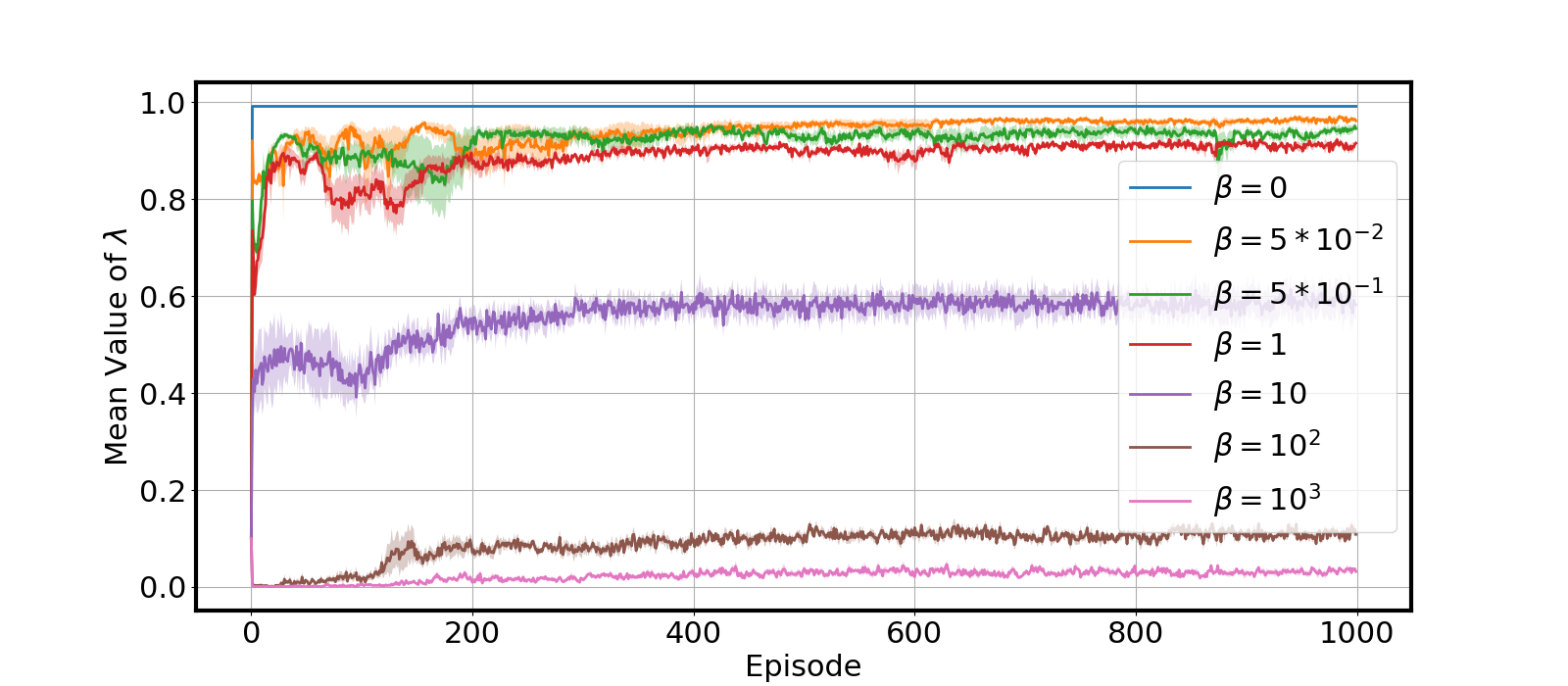
With the basic settings described above, we study how the hyper-parameter affects the empirical heuristic budget . This choice influences the average rewards, projection radii, and absolute sampled TD error reported below.
We set the unknown to be tracked as a rose-shaped trajectory shown in Figure 3:
| (16) |
We vary from to . When , the empirical implementation is the same as pure DDPG. When , we directly apply the MPC baseline. Arbitrary exploration in the action space will lead to unstable states, causing the pure DDPG to remain non-convergent throughout its training process. From our experiments, we observe that setting between and yields the largest average reward. The results are summarized in Figure 4. Under the projection rule, the action used in the experiments at each time can be written as
where serves as a trust coefficient between and . Figure 5 illustrates averaged over all time steps and tests. Figure 6 displays the average absolute sampled TD error for different choices of . This quantity visibly stabilizes when , which also yields high average rewards in Figure 4. It’s worth noting, however, that we did not actively optimize for .

Non-Stationary Environment
In a subsequent experiment, we address scenarios where there is a distribution shift in the underlying MDP. We use the same matrices , and in (14) and (15).
For each in (13), we treat it as an independent Gaussian vector. Specifically, every entry of is considered as an independent Gaussian random variable. For the first episodes, each is sampled from a normal distribution where and . However, in the last episodes, we adjust to .
In the context of this nonstationary MDP, Figure 7 illustrates the reward recovery after the occurrence of a distribution shift for varying choices of in the empirical heuristic budget . The two top figures show the average rewards. The top left figure uses the action space , while the top right uses . The bottom left figure presents the average behavior of , and the bottom right presents the average absolute sampled TD error for . With for and for , these tests show a favorable empirical balance between reward before the shift and recovery afterward. These observations concern the empirical heuristic and should not be interpreted as validating the corrected Grey Box theorem. As in the first set of experiments, we did not explicitly tune .
Appendix B Useful Lemmas
In this appendix, we present results that will be used when proving our main theorems.
B.1 Perturbation Lemma
We first prove the following perturbation lemma as a robustness guarantee, which holds for both the black-box (Section 4.1) and grey-box (Section 4.2) settings.
Lemma 2 (Perturbation Lemma).
Proof.
Our proof consists of two parts. We first bound the Wasserstein distance between joint action-state distributions for the robust baseline and PROP. Next, we bound the dynamic regret.
Step 1. Wasserstein Distance between Joint Action-State Distributions. Denote by and the PROP policy and the robust baseline. Enlarge to if necessary and adjust accordingly. Let and be their state-action laws at time . For , define the hybrid law by using through time and afterward. Thus and . The triangle inequality gives
| (17) |
The two hybrids in the th term have the same state law at time and differ only in the action applied there. Coupling them through the common state gives
| (18) |
Propagating both coupled laws with the baseline from time to time and applying Definition 3 yields
| (19) |
| (20) |
Step 2. Dynamic Regret Analysis. Since the cost functions are Lipschitz continuous with a Lipschitz constant , using the Kantorovich-Rubinstein duality theorem [34], since for all , for all ,
| (21) |
where denotes the Lipschitz semi-norm and the supremum is over all Lipschitz continuous functions with a Lipschitz constant . Therefore, the difference between the expected cost of Algorithm 1, denoted by , and the baseline policy satisfies
| (22) |
where we have used the assumption of the -locally robustness policy so that for some constant . Moreover, since the robust baseline has a ratio of expectations bound such that Using Assumption 1, from (22), we obtain
The projection identity also gives
∎
B.2 Projection Lemma
The following lemma implies a useful consistency bound. It is worth noting that the lemma also holds if PROP adopts an alternative approach instead of projecting the actions as shown in (5):
Implementing the projection rule in PROP can significantly reduce computational complexity, particularly when dealing with non-convex Q-advice.
Lemma 3 (Projection Lemma).
Proof.
Choose and define
If , convexity makes the radial point at distance from feasible, and the reverse triangle inequality shows that it minimizes the distance to . The tie-breaking rule in (5) selects this point. If , the advised action is feasible. Therefore
Lipschitz continuity of now gives
which proves the claim. ∎
B.3 Analysis of Approximate TD-Error
The following result that rewrites the approximate TD-error (c.f. (6)) is useful.
Lemma 4.
Consider the approximate TD-error in (6) and assume that the displayed variables below are integrable. Suppose
It follows that for any ,
where and are defined as
Proof.
Let and . For , let contain the history, advice, and policy randomness through the selected pair , immediately before is sampled, and define
| (24) |
The Bellman equation gives
Adding and subtracting and in the definition of gives the pathwise identity
| (25) |
Assuming integrability, since , . Taking expectations proves the stated identity. If and , then
| (26) | ||||
| (27) |
The first equality follows by summing . The second is an equivalent rearrangement.
Appendix C Black-Box Consistency and Robustness Analysis
C.1 Proof of Theorem 5.1
Theorem C.1.
Suppose the machine-learned policy is -consistent. The expected dynamic regret of PROP with the Black-Box Procedure is bounded by
where is defined in (4), is the diameter of the action space , is the length of the time horizon, is the ratio of expectations of the robust baseline , and is a hyper-parameter.
Consistency Analysis. To show the first bound in Theorem 5.1 regarding the consistency result, we consider the following steps. For any , denote by the corresponding state and action generated by the projection pursuit policy PROP, denoted by . The Bellman optimality equations (3) imply:
| (30) |
Therefore the dynamic regret of the projection pursuit policy can be rewritten as
| (31) |
Combining (31) with (30), we obtain the following cost-difference bound:
Recall that for the Black-Box Procedure in Section 4.1, the robustness budget is set as for all . Applying the bound in Lemma 3 gives the following consistency bound:
since for all , and
Noting that the machine-learned policy is -consistent, we obtain . Hence,
| (32) |
Robustness Analysis. Note that for any , , where is the diameter of the compact action space . Hence, noting the black-box setting of the robustness budget for all and applying Lemma 2, the sum of expected discrepancies, over all can be bounded by
| (33) |
C.2 Proof of Theorem 5.2
Let be the set of all MDP models satisfying Assumption 1,2, and 3. To prove Theorem 5.2, noting that by the definitions of consistency and robustness, we apply Theorem 5.1 to derive a bound on the worst-case ratio of expectations:
which implies that PROP with the Black-Box Procedure is -consistent and -robust.
C.3 Proof of Theorem 5.3
Proof.
According to Lemma 3, the expected dynamic regret of PROP satisfies
where denotes PROP. For notational simplicity, we introduce the following notation:
With the Black-Box Procedure, we set with some hyper-parameter . Therefore, there exists Lipschitz continuous Q-value predictions with a Lipschitz constant such that
| (34) |
First, we verify that Wasserstein robust policies exist since we can construct a transition probability such that the states in different times are independent. Denote by the expected optimal total cost. We can construct cost functions that are Lipschitz continuous with a Lipschitz constant and Q-advice satisfying
Note that the corresponding Q-value predictions satisfy Assumption 3. Let be the set of all MDP models satisfying Assumption 1,2, and 3. Combining above with (34), and noting that in Assumption 1, for all , , and , for any , the ratio of expectations can be bounded by
which implies that PROP cannot be both -consistent and -robust for any . ∎
Appendix D Grey-Box Consistency and Robustness Analysis
In the following, we present a dynamic regret bound for the grey-box setting (Section 4.2) that is analogous to the one presented in Theorem 5.1 for the black-box scenario.
First, in addition to Definition 4, we further recall the following quantities used in Lemma 4 for notational convenience:
| (35) | ||||
| (36) |
where by definition, and depend on the random trajectory . Denote .
Note that when the environment is stationary, under some model assumptions and with a Reproducing kernel Hilbert space (RKHS) being the function class, the optimism lemma (Lemma 5.2) in [69] shows that with probability at least , the generated Q-value functions satisfy where is the number of episodes and omits logarithmic terms and is the maximal information gain [62] that characterizes the intrinsic complexity of the function class.
Theorem D.1 (Grey-Box: Dynamic Regret).
Consider any MDP model satisfying Assumption 1,2, and 3. The expected dynamic regret of PROP (Algorithm 1) with the Grey-Box Procedure satisfies the following bounds:
| (37) | ||||
| (38) |
Consequently, the minimum of the two global right-hand sides is also an upper bound.
For the budget in (9), the two bounds imply
| (39) |
D.1 Proof of Theorem D.1
D.2 Proof of Theorem 5.4
Conditions and finite horizon bounds.
Consider a class of horizon- MDPs satisfying Assumptions 1, 2, and 3, with constants uniform over the class. Suppose there are constants such that
for every , , and , so . Let and be the Bellman innovation and martingale in Lemma 4. Assume that a deterministic nondecreasing boundary , with , satisfies
uniformly over the admissible adaptive policies. Write . Finally, define
with , and suppose the baseline guarantee is restartable in the sense that, for a class-uniform ,
| (40) |
for every and every reachable .
For each horizon, set in the Grey-Box Procedure. Let and
The consistency factor under exact Q-value advice and the robustness factor over the admissible advice class are respectively bounded by
| (41) |
Consequently, Theorem 5.4 follows if , , , and , together with and stated above.
The confidence condition is a concrete property of and . For example, if the innovations are conditionally -sub-Gaussian uniformly over the class, one may take
Uniformly Lipschitz and transition distributions with uniformly bounded support diameter give such a condition by Hoeffding’s lemma. If , , and is fixed, then the two factors in (41) are
Condition (40) makes explicit that the baseline guarantee must hold after a data-dependent switching time. It holds whenever the same baseline ratio applies uniformly to every restarted suffix MDP, up to the sublinear term .
Proof.
Let
By assumption, . We first record two pathwise bounds. The projection identity and the Lipschitz continuity of give
| (42) |
Moreover, Assumption 3 gives
| (43) |
Let
with if the set is empty. Since is nondecreasing and , Equation (9) gives for every . Thus PROP follows the baseline from onward.
On , the accumulated advantage before the switch satisfies
| (44) |
To see this, if , then and hence . Equation (29) gives
The crossing action satisfies by (43), which proves (44). The case follows directly from (43). If , the same argument at time , followed by the bound on the final action , proves (44). On , Equation (43) gives . Therefore
| (45) |
The time is a bounded stopping time for the trajectory filtration. With , optional stopping in the Bellman performance-difference identity gives
| (46) |
Applying the restartable baseline bound (40) conditionally at and using nonnegative costs,
Combining this inequality with (45) and proves the robustness factor in (41).
Finally, suppose the Q-value advice is exact. On , induction gives , , , and for every . Indeed, this is true at . If it is true before time , Equation (29) gives , so the next action again follows the optimal Q-value advice. Hence on . On its complement, exact advice and (43) give . The performance-difference identity therefore yields
Dividing by proves the consistency factor. If transitions are deterministic, then and the same induction gives exact consistency without a failure event.
Appendix E Proof of Theorem A.1
To show Theorem A.1, we first show a technical lemma with respect to , which plans until the end of the episode from the first time step.
Lemma 5.
Proof.
To simplify the notation, we define
| (47) |
By the KKT conditions, we see that for any , the predictive optimal solution is given by
Therefore, is a linear function of , and this relationship defines . Lemma G.2 in [42] implies that . Note that the block matrix is invertible since and are positive definite.
To simplify the notation, we define the state transition matrix
Consider an arbitrary state . Note that is the optimal trajectory when there is no disturbance after step . By the principle of optimality, we see that is identical with the actual trajectory of after step . In other words, for arbitrary , the multi-step transition matrix satisfies
Lemma G.2 in [42] implies that . ∎
Lemma 5 shows that has the same effect as a time-varying linear feedback controller that is exponentially stable. We generalize this property to with a smaller prediction horizon (Lemma 6) by showing that behaves similar to when is sufficiently large.
Lemma 6.
Proof.
Let . By the KKT conditions, we see that for any , the predictive optimal solution is given by
Therefore, is a linear function of , and this relationship defines . By Lemma G.2 of [42], we see that .
When , construct an auxiliary disturbance sequence with and for all . We see that
Therefore, we see that
| (80a) | ||||
| (80b) | ||||
where we have applied the perturbation bounds in Lemma G.2 of [42] in (80a) and (80b). Since this inequality holds for any arbitrary , we see that . To simplify the notation, we denote .
To establish a dynamic regret bound that depends on the offline optimal cost, we first need to show a lower bound of that depends on the “power” of the unknown disturbances.
Lemma 7.
The offline optimal cost is lower bounded by
Proof.
Note that the dynamics of the LTV system can be rewritten as
Taking norms on both sides of the equality gives
| (82a) | ||||
| (82b) | ||||
where we have used the triangle inequality in (82a) and the definition of the induced matrix -norm in (82b). Taking the squares of both sides and applying the Cauchy-Schwartz inequality together imply
| (83) |
By (83) and the assumptions on and , we obtain that
Since the above inequality holds for any arbitrary trajectory , we conclude that Lemma 7 holds. ∎
Since the Wasserstein robustness (see Definition 3) is for distributions on the state-action space, we also prove a technical lemma below that helps convert the contraction on deterministic state/action pairs to the contraction on distributions. Let denote the Wasserstein -distance between two distributions and .
Lemma 8.
Suppose is a deterministic function that satisfies for any . Then, for any pair of distributions and on , we have .
Proof.
Recall that , where is a joint distribution on with marginals and . We define a mapping as . We see that gives a joint distribution on with marginals and , and it satisfies
Note that the above inequality holds for any with marginals and . Thus Lemma 8 holds. ∎
Now we are ready to show Theorem A.1.
For a state at time step , let and denote the corresponding state and action of MPC at time step . By Lemma 6, we see that for any state-action pairs and at step , we have
| (84a) | ||||
| (84b) | ||||
| (84c) | ||||
where we have used Lemma 6 in (84a) and (84b); Moreover, we have applied the assumption that and and the triangle inequality in (84c). Since (84) establishes a contraction for a deterministic state-action pair and the dynamics is deterministic, applying Lemma 8 finishes the proof of the first conclusion of Theorem A.1.
Using a similar decomposition technique with [42], by Lemma 6, we see that the trajectory of PROP satisfies that
| (85) |
where we denote and the assumption that PROP deviates at most from ’s action. We also see that
| (86) |
This finishes the proof of the second statement in Theorem A.1.
Let the trajectory of when executed without the machine-learned advice be denoted by . We see that
Applying the Cauchy-Schwarz inequality, we obtain
| (87) |
For the control actions of , we also see that
| (88) |
Therefore, we get the following bound on the total cost:
| (89a) | ||||
| (89b) | ||||
where we have used the assumption that and in (89a); we have also used the inequalities (E) and (88) in (89b). Combining (89) with the lower bound of in Lemma 7 finishes the proof of the third Statement in Theorem A.1.
Appendix F Proof of Theorem A.2
Before showing Theorem A.2, we first state a technical lemma that establishes the relationship between the TV distance and the Wasserstein distance.
Lemma 9.
For any distributions on , we have
Proof.
To see this, note that since for any , the Wasserstein -distance equals 2 times the probability mass we need to transport to convert to . For every such that , we need to move out exactly from the probability mass at to other points . Therefore, we must have
∎
Note that the MDP’s transition kernel acts as a deterministic function. It maps the current state-action pair from to the distribution of the subsequent state in . Hence, the current state-action distribution on maps to a distribution on . To proceed with this recursion, we require the distribution of the next state, which should be on . This is in contrast to needing the distribution of the distribution of the next state, which would be on . Therefore, to convert the distributions on back to distributions on , we require the following lemma.
Lemma 10.
Let be two distributions on . It follows that .
Note that and are distributions on .
Proof.
By the definition of the Wasserstein distance, we have
where is a joint distribution on with marginals and . For any such joint distribution , we have
This finishes the proof of Lemma 10. ∎
We now resume our discussion with the proof of Theorem A.2.
Given the state-action distribution at step , let denote the resulting state distribution at step . We slightly abuse the notation so that for any pair , still outputs the resulting state distribution at step . We see that
Therefore, by Lemmas 8 and 10, we see that
| (90) |
Note that Lemma 1 and Lemma 9 imply that
Combining this with (90) gives that
| (91) |
For any distributions on , we also see that , which implies
Substituting this into (91) gives that
validating that the Wasserstein robustness (Definition 3) is satisfied.