Correlation networks, dynamic factor models
and community detection
AMS subject classification: Primary: 62M10, 62H30, 05C22. Secondary: 62H20.Keywords and phrases: Time series, dynamic factor model, loadings, mixture distribution, correlation matrix, network, communities, -means. The first and third authors were supported in part by the NSF grants DMS-2113662 and DMS-2134107. The second author was supported in part by NSF grant DMS-2134107.
Abstract
A dynamic factor model with a mixture distribution of the loadings is introduced and studied for multivariate, possibly high-dimensional time series. The correlation matrix of the model exhibits a block structure, reminiscent of correlation patterns for many real multivariate time series. A standard -means algorithm on the loadings estimated through principal components is used to cluster component time series into communities with accompanying bounds on the misclustering rate. This is one standard method of community detection applied to correlation matrices viewed as weighted networks. This work puts a mixture model, a dynamic factor model and network community detection in one interconnected framework. Performance of the proposed methodology is illustrated on simulated and real data.
1 Introduction
Community detection methods for weighted networks have been applied extensively to correlation matrices of time series data Gates et al. 2016; MacMahon and Garlaschelli 2015; Masuda 2018; Zhang and Horvath 2005; Worsley et al. 2005. Conceptually similar procedures have also been formulated based on various forms of hierarchical clustering of correlation matrices Liu et al. 2012. This is often carried out in a way that is agnostic to an underlying data generating model (for which the correlation matrix is computed), with limited theoretical guarantees on the validity of community detection. In this work, we propose one natural model for the data generating process, define the notion of community explicitly, consider a standard community detection method and provide results for its performance under the model.
The proposed model builds on a (dynamic) factor model for a -vector stationary time series driven by a low-dimensional -vector stationary factor series , where refers to discrete time. The connection to communities is postulated through a loading matrix consisting of rows , with column vectors . (All vectors in this work are assumed to be column vectors and prime indicates transpose.) We assume that ’s are drawn from a distribution on (in fact, a unit disc in ), and say that the model has communities when is a mixture of distributions . For identifiability purposes, we require that the means of are distinct. More precise assumptions on are given in Section 3.2.2. The component is in community when is drawn from . The exact model, called Community Dynamic Factor Model (CDFM), is defined in Section 2 below.
We examine a number of issues for the CDFM: the block structure of the resulting correlation matrix, parametric mixing distributions , extensions to covariance matrices rather than correlation matrices, connections to other related constructions such as random dot product networks Young and Scheinerman 2007; Athreya et al. 2018 and reduced-rank Vector AutoRegressive (VAR) models. We also consider model estimation, including community detection methods, focusing on the standard spectral clustering through -means, for which we apply a general theoretical result on the misclustering rate, obtained in Patel et al. 2023, for the CDFM setting.
The construction of the CDFM is motivated in part by the apparent block structure of correlation matrices for many multivariate time series. Several such matrices are examined in connection to the model, where we are particularly interested in the presence of mixing distributions (communities) and the dependence of clustering on separation of the mixing distributions. Applications presented in Section 4 below concern macroeconomic time series and fMRI data.
The construction of the CDFM is conceptually simple and connected to other approaches. The loading matrix will be estimated below through principal components of the correlation matrix. Thinking about mixtures and clustering of principle components is certainly not new, especially in the applied context Jolliffe 2002. On the other hand, correlation matrices can be viewed as weighted networks, amenable to network analyses. Our key contribution is that the CDFM allows us to connect a mixture model, a dynamic factor model (and principal components) and network community detection in one framework.
It should be noted that the proposed framework and the results could also be cast in a multivariate, non-time series context, where time is replaced by index , associated for example with different subjects, and where factors are thought as i.i.d. across . We work in the time series context for several reasons. Our own research interests aside, the stationary factors do not need to be independent across time in the time series context. When follow a Vector AutoRegressive (VAR) model, the CDFM is related to large VAR models with network structure, as we discuss in this work (Section 5). Our applications are also for time series (Section 4), and interesting future directions (e.g. change point detection) concern specifically data with temporal ordering.
The rest of the paper is structured as follows. The CDFM is formulated and studied in Section 2. Estimation and community detection for the CDFM are considered in Section 3. Simulations and applications to real data can be found in Section 4. Connections to other constructions are discussed in Section 5. We conclude in Section 6 and technical assumptions are stated in Appendix A.
2 Community Dynamic Factor Model
2.1 Model Formulation
Let denote the node set. Let be a -dimensional stationary time series following a dynamic factor model (DFM), and more specifically its so-called static form Stock and Watson 2016 given by
| (2.1) |
where is an -dimensional stationary time series, is a loadings matrix with row vectors and , and are the error terms with and . The factors can be dependent across time and are assumed to have zero mean. The errors and factors are assumed independent with further assumptions stated below in connection to the theoretical results. As common in the DFM literature, we mitigate the issue of non-identifiability of the DFM by assuming
| (2.2) |
so that are now identified up to an orthogonal transformation (specified in Section 3.1). We shall also discuss the case when (2.2) is not assumed in Section 2.4.
For the loadings, fix , distinct probability measures on and a probability mass function . Consider the mixture distribution
| (2.3) |
The loading rows are assumed to be independent and
| (2.4) |
that is, ’s are drawn independently from .
Definition 2.1.
Further technical assumptions are specified in Section 3.2.2; for the moment, the reader can think of the mixing distributions as point masses, Gaussian distributions or other unimodal distributions with distinct location parameters. We also assume that ’s are drawn and fixed. In particular, the expectation sign throughout stands for the conditional expectation given , and for the expectation with respect to the randomness in the loadings .
Assume that the component series are normalized, so that
| (2.5) |
Since
| (2.6) |
we must have that . This constraints the mixing distributions to the unit disc . Furthermore, this assumption enforces that the correlation matrix and the covariance matrix (conditional on the loadings) are the same and given by
| (2.7) |
by using (2.2). Write
| (2.8) |
for the sample covariance matrix, where the sample mean is not subtracted for simplicity. We also ignore the issue of standardization of data. The sample covariance will not be used until Section 3.
The individual components of the time series are driven by the loadings drawn from mixing distributions. Naturally, one can group the components into communities given by the respective distributions of the rows of .
Definition 2.2.
Let be the membership matrix given by if is drawn from and otherwise. Let be the membership function given by if and otherwise. Communities for the components are defined as , . Define to be the size of community .
2.2 Block Structure of Correlation Matrices
A feature of the CDFM is that its correlation matrix will have a block structure on “average.” In practice, possibly after reordering by communities, sample correlation matrices do often exhibit block structure. This suggests our model as a candidate to capture this phenomenon.
Indeed, assume that the component series of are ordered by community membership so that
| (2.9) |
where is a vector of ’s and ’s are vectors of ’s of the appropriate dimensions. The community structure in translates into the block structure of the component of the correlation matrix on “average” as follows. Under the mixture measure, given in (2.9), the expected is a block matrix given by
| (2.10) |
where is a matrix of ’s and
| (2.11) |
are the means of the mixing distributions. The main diagonal blocks of (2.10) are characterized by the inner products of the means . If the inner products are unique, then the main diagonal structure is sufficient for community identifiability. Although this is sufficient, it is not necessary. In fact, even if for some , we have that , as long as there exists an such that , we will still see the community block structure in .
Two other observations are worth making. First, the only restriction is . Second, what determines the number of blocks is (the number of mixing distributions), not (the number of factors). That is, one can have a block matrix even for one factor as in examples in Section 2.6.
2.3 Case of Covariance Matrices
We focused above on correlation matrices assuming that . Without this assumption the covariance matrices can, in principle, be treated similarly. In fact, the discussion simplifies in that the mixing distributions can now be on (instead of . A popular Gaussian mixture distribution can be considered for .
However, this model for presents interpretation issues: is the block (community) structure now driven by the variances or the correlations or some combination of the two? For example, when , and for some , , where we take . If is small relative to , especially for large ’s, . So the variances contain the community information. However, the correlations,
| (2.12) |
contain little community information. If is comparable to , then the correlations also contain the community structure.
For this interpretation reason and also since sample correlation matrices are usually of interest in practice, we advocate to work with correlation matrices. The community structure on variances could also be of interest, and can be studied through other means.
Finally, we also note that the relationship between covariance and correlation matrices is akin to the relationship between the adjacency matrices of networks and their degree corrected counterparts. Let , with for simplicity, be the adjacency matrix of a weighted network. The degree corrected adjacency matrix is
where is the degree of node and (Karrer and Newman 2011). For correlation matrices, the variance plays the role of the degree. Furthermore, as the properties of the covariance matrix can be dictated by the variances according to the discussion above, the same holds for node degrees in adjacency matrices. For example, without degree correction, it is known that the distribution of the eigenvalues of the adjacency matrix follow that of the degrees, even if there is an underlying community structure (Zhan et al. 2010).
2.4 Case of Non-Orthogonal Factors and Effect of Rotations
We assumed in (2.2) that the factors are orthogonal, motivated in part by the principal component analysis (PCA) used below, which yields this orthogonality. If (2.2) is not satisfied, the covariance of is given by . Letting be the eigendecomposition with orthogonal and diagonal , and , the DFM (2.1) can be written as with and . Note that the transformation does not necessarily preserve angles. See Example 2.3 for such a case.
Another aspect of the above transformation to keep in mind is that can be sparser than and thus potentially more interpretable (or vice versa). It should be noted that the issue of sparsity of is pertinent for orthogonal factors as well. The orthogonality of factors is preserved under orthogonal transformation (e.g. rotation), but the resulting can indeed become sparser. This is the basis of the traditional VARIMAX procedure (see Rohe and Zeng 2023 for a more modern take). More generally, estimation of sparse loadings is the objective of sparse PCA and related approaches Guerra-Urzola et al. 2021. The focus of this work will be on orthogonal factors and for identifiability purposes, we shall focus on a specific rotation such that
| (2.13) |
for some diagonal matrix . Indeed, the DFM is identifiable when imposing the constraints (2.2), (2.13), and that the entries of are distinct.
2.5 Parametric Families of Mixing Distributions
The mixture model with the assumptions above restricts the distributions to the unit disc . In this section, we discuss some parametric families of mixing distributions on . The discussion below concerns properties of a typical component of the mixture, so we drop from the notation for simplicity. We also replace by a general random variable in the discussion below.
2.5.1 Point Mass
The simplest family of mixing distributions is the point mass family where each mixing distribution has all of its mass on , i.e. . As long as the points are distinct, the mixture is identifiable. Point mass mixtures are a common choice of mixing distributions as they allow constant values within communities. For example, in the Random Dot Product Graph (RDPG) literature, it is often assumed that the latent attributes of nodes from a single community are constant. More details on RDPGs and their connections to the CDFM are provided in Section 5.1.
2.5.2 Projected Normal Distribution
Let , the -dimensional normal distribution with mean and covariance , and define . Then, is distributed as a projected normal distribution (PND), . The PND is a unimodal and symmetric distribution on with mean . The PND has identifiability issues: for any constant , has the same distribution as .
To construct distributions on , let where with is independent of . One may take to follow other parametric unimodal distributions on . Then, follows a unimodal distribution on . See Example 2.5 for a numerical illustration of a model from this class.
2.5.3 Restricted Normal Distribution
Let with positive definite . The restriction of to the unit disc, denoted , has a probability distribution function (pdf) given by
| (2.14) |
where is the pdf of . To calculate , one notes that is of quadratic form and hence the distribution can be calculated explicitly as follows. Let be the eigendecomposition with orthogonal and diagonal . Then, has a generalized chi-squared distribution,
| (2.15) |
where are independent non-central chi-squared distributions with the non-centrality parameters given by the vector Mathai and Provost 1992. Following Imhof 1961, when the eigenvalues of are assumed to be unique, the CDF of can eb expressed as
| (2.16) |
where
| (2.17) | ||||
| (2.18) |
and . The expression (2.16) can be used to compute in (2.14).
2.6 Examples of CDFMs
We illustrate the various concepts introduced above through several examples of CDFMs.
Example 2.3.
Consider . Fix with and
| (2.19) |
where , the uniform distribution on , independent across indices with . Thus, we assume that , , for community 1 are drawn from and , for community 2 from . The cross correlation term controls the dependence between the strengths of nodes in communities 1 and 2. A distributionally equivalent representation is given by moving from to as
| (2.20) |
Now, the dependence of the factors is put on the mixing distributions as and . The effects of can be seen in Figure 2.1. Note that as increases, we lose separability of the two communities. The model (2.19) appears in Gates et al. 2016.
The number of factors does not need to equal the number of communities . The following are simple examples with .
Example 2.4.
Let and . Take with i.i.d. and . Equivalently, with and . This is a similar construction to the parametric family defined in Section 2.5.2.
Consider another setting where and , let and . Then each is either or depending on its community assignment.
Let , the -dimensional normal distribution with mean and covariance , and define . Then, is distributed as a projected normal distribution (PND), . The PND is a unimodal and symmetric distribution on with mean . The PND has identifiability issues: for any constant , has the same distribution as .
To construct distributions on , let where with is independent of . One may take to follow other parametric unimodal distributions on . Then, follows a unimodal distribution on . See Example 2.5 for a numerical illustration of a model from this class.
Example 2.5.
Consider the PND-Beta distribution as described in Section 2.5.2. Let and , , for with independent of . Define and
| (2.21) |
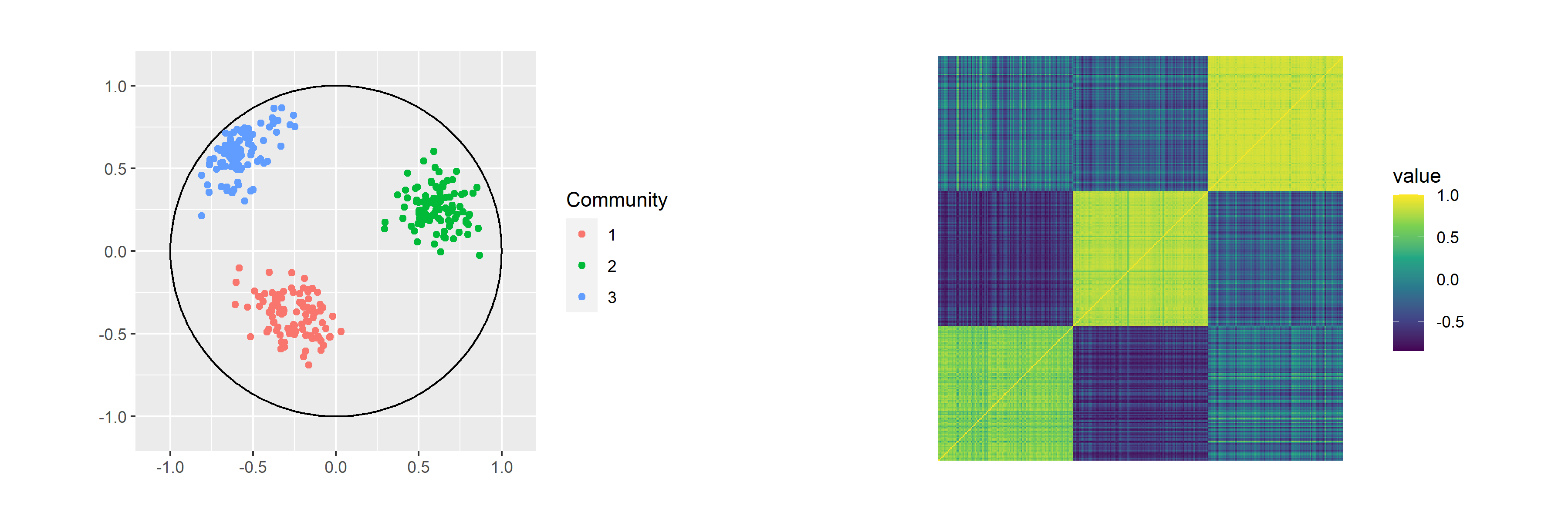
So, is a distribution on such that for any vector sampled from , the angle is determined by the normal distribution and the magnitude is determined by . As an example, take and . Set , , and . We sample 100 vectors from each of for . The plots of and are shown in Figure 2.2. Note that, even though the main block diagonal does not clearly show three communities (but rather two communities), the off diagonal blocks show three communities.
Remark 2.1.
In view of (2.6), the closer is to the unit circle, the stronger the “signal” is in the component series (equivalently, the weaker the noise ). This also means that the closer ’s from a community are to the unit circle, the stronger the correlations will be among the component series ’s. This can be seen in Figure 2.2, where community 3 (blue) is closest to the unit circle and has the correlation block (top right) with the largest values. This perspective should also be kept in mind with estimated loadings in practice, as in the data illustrations in Section 4.
3 Estimation and Community Detection
We discuss here estimation questions for the CDFM, including estimation of communities. We work in the regime where both the dimension and the sample size can be large. We assume throughout that the number of factors and the number of communities are known. In Section 3.2.3 below, we discuss one method to choose in practice and refer the reader to Stock and Watson 2016 for methods to pick .
3.1 Loading and Factor Estimation
We recall here several known results on estimation of loading matrix and factors , as needed for subsequent community detection. The loadings and factors are estimated through a standard PCA approach as follows. Let be the eigendecomposition of the sample covariance matrix (2.8) where consists of the orthogonal eigenvectors and the diagonal matrix consists of the respective eigenvalues, in decreasing order. Let be the matrix of the first eigenvectors of associated with the largest eigenvalues forming a diagonal matrix . The PCA estimators are defined as
| (3.1) |
Note that, by construction,
| (3.2) |
The constraints (3.2) allow one to identify the limits of and in terms of and . More specifically, let
| (3.3) |
be the eigendecomposition of . (Do not confuse and ; even their dimensions are different.) Then, . Since is diagonal as is the first relation in (3.2), under suitable assumptions (Bai and Ng 2008 and Doz et al. 2012), as ,
| (3.4) |
where is the spectral (operator) norm, , and . Strictly speaking, the eigenvalues in need to be different for this identifiability (see also (2.13)) and one of the key assumptions is that of strong factors, essentially saying that the eigenvalues of need to be of the order , which we express as
| (3.5) |
Bai and Ng 2008 and Doz et al. 2012 provide convergence rates for (3.4) as well.
For our results on community detection, we shall need the following stronger convergence result.
Proposition 3.1.
[Uematsu and Yamagata 2023, Lemma 6] Let be an arbitrary constant. Under suitable assumptions on the DFM (2.1), with probability at least ,
| (3.6) |
for some , where .
3.2 Community Detection Through -Means
By (3.4) and (3.6), PCA estimates the rotated loadings matrix . Rotation preserves the mixture structure (2.3), with each mixing distribution undergoing the same rotation. To simplify the notation, we shall drop the superscript from and simply write for the loading matrix estimated through PCA.
We are interested here in estimating the communities in Definition 2.2. With known (or ’s), a commonly used algorithm for clustering is -means, which we recall in Section 3.2.1 below. Theoretical results on misclassification rate are derived in Patel et al. 2023 by considering estimated loadings as perturbations of the original loadings under the assumption that the mixing distributions are well-separated. In Section 3.2.2, we apply one of these results to the case where ’s are thought of as perturbations of ’s of magnitude at most the bound in (3.6). Throughout we assume is known, deferring the reader to Section 3.2.3 for methodology to pick .
The terms “cluster” and “community” will be used interchangeably, especially in connection to -means, and should be understood as such.
3.2.1 -Means Algorithm
The -means clustering technique aims to cluster a set of points : into clusters (communities) , by minimizing
| (3.8) |
where is referred to as an estimated clustering, denotes an estimated cluster assignment (i.e. if ) and is the mean of the points in .
The -means optimization problem is NP-hard Mahajan et al. 2009 and is tackled by a class of algorithms which attempt to approximately minimize (3.8) by initializing a set of candidate means, then iterating between updating cluster assignments and updating cluster means. One of the most popular and simplest algorithms is Lloyd’s algorithm Lloyd 1982, often referred to as the standard or naive -means. The updating step in Lloyd’s algorithm is as follows. Let be the means of the cluster assignments at the -th iteration. Then, the cluster assignment of at the -th iteration is given by
| (3.9) |
Lloyd’s algorithm converges to a local minimum but is reliant on good initialization to achieve a global minimum. Lloyd’s algorithm is often initialized as follows. Sample randomly from . For the remaining points, calculate the distance squared to the closest initialized mean and sample from the remaining points with probability proportional to this squared distance. Repeat the procedure until all means have been initialized. Lloyd’s algorithm initialized in such a way is referred to as the -means++ algorithm (Arthur and Vassilvitskii 2007). For an overview of the -means algorithm and its variants, see Wierzchoń and Kłopotek 2018.
3.2.2 -Means for CDFM
To estimate the communities in the CDFM, we apply -means to the obtained PCA estimates . This setting differs from most -means settings in the mixture model literature McNicholas 2016 as we are estimating, not observing, the draws from the mixture. We will focus on the performance of Lloyd’s algorithm on the CDFM using results established in Patel et al. 2023. We first need some notations and assumptions.
We will assume that each mixing distribution for is sub-Gaussian with the same sub-Gaussian parameter and write . In other words, for and ,
| (3.10) |
Note that this assumption controls the concentration of even for supported on . Let and be the estimated means and community membership function after iterations of Lloyd’s algorithm applied to ’s. Recall from Definition 2.2 that denotes the true community membership function. Define the misclustering rate at step as
| (3.11) |
Recall that denotes the mean of as defined is (2.11). Define the minimal and maximal distance between the true cluster means as
| (3.12) |
In view of (3.6), define
| (3.13) |
i.e. the maximal error between the true and estimated loadings. Let be the minimum cluster size proportion and define the sub-Gaussian and estimation error signal-to-noise ratios as
| (3.14) |
respectively. Define as
| (3.15) |
Note that as .
Then, given that is a sub-Gaussian mixture, Patel et al. 2023, building on the work of Lu and Zhou 2016, prove Theorem 3.2 below about the clustering accuracy of Lloyd’s algorithm on assuming good initialization. The condition on the initialization of Lloyd’s algorithm requires either the cluster-wise misclustering rate or the maximal distance between the true and estimated cluster means to be small enough.
More precisely, define as the initial community membership function given to Lloyd’s algorithm and set
| (3.16) |
to be the set of loadings in community which are initially misclustered into community . Define , , and the cluster-wise misclustering as
| (3.17) |
where is the true size of community . Then, an initial community membership with initial means is considered good enough if either one of the following hold:
| (3.18) |
Note the initialization condition weakens as both signal-to-noise ratios increase.
Theorem 3.2.
[Patel et al. 2023] Assume that , , , for some sufficiently large constants . Conditional on a good enough initialization, we have
| (3.19) |
with probability greater than .
Note that the bound on the misclustering rate depends on both the effective sub-Gaussian and estimation error signal-to-noise ratios. The final max term in the error bounds indicates that it is not good enough to have just one of the terms be small. We must have good estimation of the loadings and sub-Gaussian error relative to the distance between the means for Lloyd’s algorithm to work well in this case. One may be puzzled by the disappearance of the length and the dimension of the time series, but note that and enter in through (3.6). Our simulations in Section 4.1 will examine the result of Theorem 3.2 from the numerical standpoint.
3.2.3 Choice of
In practice, it is often the case that researchers choose to equal based on the scree plot of the eigenvalues of the correlation matrix. However, as shown in Example 2.4, it may be the case that and choosing may lose significant information. Thus, given , we need suitable methodology for picking . We use SigClust Liu et al. 2008, a procedure which tests whether the data come from a single normal distribution to judge the significance of clustering.
The procedure for SigClust is as follows. First, we initialize SigClust by assigning two communities to the data. We choose to do so with Lloyd’s algorithm with . Then SigClust simulates the data multiple times by sampling i.i.d. observations from the estimated null distribution. For each simulation, SigClust calculates the Cluster Index (CI), the sum of within community variation over the total variation, based on the initial community assignments. The simulated CI distribution is compared with the observed CI in the data. Lastly, a -value obtained as a quantile from the empirical distribution of cluster indexes is given.
We apply SigClust iteratively on estimated loadings. More precisely, we run SigClust on , with initial two communities given by Lloyd’s algorithm. If the outputted -value is larger than some predetermined threshold , we conclude and determine . Otherwise, we split the estimated loadings into two groups based on the initialized community assignments. Then for each group we repeat the SigClust procedure separately. Once the procedure ends, we choose to be the number of groups the loadings were split into. Note that this procedure not only picks but also clusters the estimated loadings. However, we only use SigClust to choose in our work. In Section 4.1.3, we examine how SigClust performs for different values of and in the CDFM. We are actively pursuing a principled approach to choosing both and simultaneously, but defer this to future work.
3.3 Parametric Estimation of Mixing Distributions
We discuss below two parametric estimation methods when the mixing distributions are the restricted normal distributions as described in Section 2.5.3: maximizing the log likelihood and noise contrastive estimation Gutmann and Hyvärinen 2010. In either case, we first perform community detection on as in Section 3.2.2. Then, for each community , we treat as an i.i.d. sample from a restricted normal distribution. We then numerically optimize the log-likelihood or the objective function of noise contrastive estimation as described below.
3.3.1 Maximizing Log-Likelihood
3.3.2 Noise Contrastive Estimation
Noise Contrastive Estimation (NCE) Gutmann and Hyvärinen 2010 allows estimating the parameters of the normal distributions without the need to calculate . This is done by creating noise data similar to the observed data, , and building a model which can differentiate between the observed and noise data. Generate noise data from a normal distribution with mean and variance . Let and denote the pdfs of and the noise distribution , respectively. One treats as a constant throughout so that is a parametric function of , , and . One then maximizes (as a function of , , and )
| (3.21) |
with respect to , , and . In Section 4.1.2, we evaluate the performance of NCE for simulated data.
4 Numerical Studies
In this section, we assess community detection and other estimation methods for both simulated and real data.
4.1 Simulations
We examine the result of Theorem 3.2 for simulated data and show the effects of and on misclustering. Also, we examine how well the SigClust procedure estimates when is known and examine performance of NCE in estimating mixing means and variances.
4.1.1 Empirical Consistency of -Means
We consider the case when for ease of visualization. We let the community sizes be equal so that . In order to control sub-Gaussian signal-to-noise ratio , we need to use distributions on whose sub-Gaussian parameter can be easily manipulated. We let , , be normal distributions restricted to centered at with variance matrix given by as detailed in Section 2.5.3. Then by definition. Furthermore, we restrict to be equidistant by requiring that , for some , and we also suppose for all . Then . So the sub-Gaussian signal-to-noise ratio in (3.14) is given by
| (4.1) |
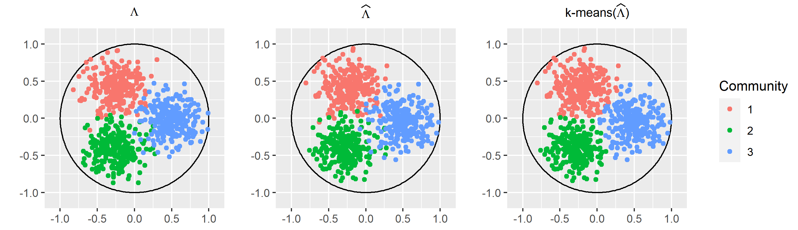
Let and be a grid of parametric choices. For each , we construct loadings following the mixture distributions described above and generate i.i.d. factors from a multivariate normal distribution with mean and variance (so there is no time dependence). The errors are similarly sampled i.i.d. from a multivariate normal distribution with mean and variance . We construct as in (2.1) and use the sample correlation matrix to obtain the PCA estimate with . We then use Lloyd’s algorithm to estimate the clustering . The misclustering rate is calculated given the true clustering. This procedure is repeated 10 times for each . An example of the procedure with is given in Figure 4.1.


The right plot of Figure 4.2 shows that the average misclustering rate decreases as or increases. Note that regardless of , as increases, misclustering decreases. This is not surprising as larger samples from a sub-Gaussian concentrate around the true mean with high probability. The left plot of Figure 4.2 shows the average misclustering rate, on the log scale, for all simulations in which and . As increases, the misclustering rate decreases and is below , one of the terms in the bound obtained in Theorem 3.2. Taking other choices of and yields a similar plot. The individual effects of and on misclustering rate are shown in Figure 4.3. The right plot of Figure 4.3 shows that as means get further apart and as noise gets smaller, misclustering rate decreases and the left plot shows that as the distance between means increases, misclustering rate decreases.
4.1.2 NCE

We consider the same setup for the simulated data as in Section 4.1.1 but with the following differences. We allow and to change but we fix and . (These values of and were chosen to be comparable to Gates et al. 2016.) We let , for some , where are i.i.d. and follow a -dimensional standard normal distribution. The covariance matrix of the mixing distribution is given by . The estimation procedure for is the same as in Section 4.1.1 with the exception that we assume the true community membership is known. For each cluster (community), we estimate the mean and variances (i.e. the diagonal of the covariance matrix) of the restricted normal distribution by numerically optimizing the NCE objective function (3.21) with initial . The mean error for each cluster is given by the norm of the estimated mean minus the true mean. The variance error for each cluster is given by the Frobenius norm of the estimated variances minus the true variances. The average mean and variance errors refer to average across clusters for each simulation.
Figure 4.4 shows the boxplots of the average mean error (left) and average variance error (right) for each choice of and . Note that for both plots we have fixed and . Thus, the true variance matrix is . Each boxplot is obtained from 400 simulations for that value of and . Note that as and increase, the average mean error increases and variation across simulations grows. However, the average variance error decreases as increases.
4.1.3 SigClust

The simulations in Section 4.1.1 and 4.1.2 assume that the true is known. In this section, we estimate using the SigClust procedure described in Section 3.2.3. We consider the same setup as that in Section 4.1.2 and we let be the -value threshold for the SigClust procedure. We define the SigClust error as where is the output of the SigClust procedure with threshold .
Figure 4.5 shows the boxplots of the SigClust error for different choices of , , and with and . For each choice of , , and , boxplots of 100 iterations of the simulation are plotted. Naturally, as increases the SigClust error also increases for all values of . Note that as grows, larger values of do as well if not better than small seeming to indicate SigClust is conservative in these settings. Further explorations are deferred to future work.
4.2 Applications
4.2.1 fMRI data
We explore our -means clustering procedure on fMRI data obtained from a subset of the Human Connectome Project Elam et al. 2021. The fMRI time series are the BOLD (blood oxygen level dependent) signals for regions of interest (ROIs) in a brain. The data here include fMRI time series for 10 individuals who are going through multiple tasks with short resting states between tasks. There are 268 ROIs with 392 time points corresponding to seconds. We focus on one subject’s fMRI scan and restrict ourselves to 58 ROIs. So, our time series has dimension and length .
The eigenvalues of the sample correlation matrix and the PCA estimates , with and community labels given by Lloyd’s algorithm with , are plotted in Figure 4.8. Figure 4.8 shows the sample correlation matrix with two different orderings. The black lines indicate separation by community. The first ordering is with respect to the Default Mode Network (DMN) and Attention Network (AN) which are two different brain networks consisting of several structural regions of the brain. The DMN is known to be one of the regions of the brain which are deactivated when during directed tasks. The AN, on the other hand, is known to be active during directed tasks. The second ordering uses the community labels obtained from Lloyd’s algorithm with , which was the estimated number of clusters using the SigClust procedure with and . Note that there is a clear block structure once we reorder using our estimated communities. In general, fMRI time series have temporal dependence. Figure 4.8 includes the sample auto-correlation functions (ACFs) of the estimated factor series.


4.2.2 Macroeconomic Data
We perform community detection on the US Quarterly data taken from the DRI/McGraw-Hill Basic Economics database of 199911 1 https://dataverse.unc.edu/dataset.xhtml?persistentId=hdl:1902.29/D-17267 which consists of macroeconomic time series sampled quarterly from 1959 to the end of 2006 resulting in . A more detailed description of the time series along with the transformations to stationarity that have been made are provided in the Data Appendix of Stock and Watson 2009.
We estimate the loading matrix using factors and perform -means with communities. The number of communities was chosen by the SigClust procedure with . The loadings projected to the first two dimensions are plotted in Figure 4.10 where the communities are distinguished using color. Figure 4.10 also shows the sample correlation matrix whose entries are reordered according to the -means algorithm. The sample correlation matrix exhibits block structure and the projection of the ’s shows separation. Some of the more interesting clusters are shown in Figure 4.10 with labels for the time series. All the time series with labels starting with “LHU” deal with unemployment rate. The time series starting with “CES” with a number less than 140 represent number of employees in different categories. The time series labeled “CES151” represents average weakly hours and overtime hours, respectively. The rest of the “CES” time series end with “R” and represent real average hourly earning for different populations and we can see a clear separation between the “CES” series with and without “R” in the loadings in Figure 4.10.


5 Connections of CDFMs to Other Constructions
5.1 Random Dot Product Graphs
Latent position random graphs Hoff et al. 2002 allow for random heterogeneous node attributes which determine relationships (edge connections) between nodes. More specifically, each node has attribute sampled from some latent space and the probability of an edge between nodes and is given by for some kernel function . One concrete example in this general class is as follows: take to be any subset of such that for all , and to be the dot product function. The corresponding latent position random graph is called the Random Dot Product Graph (RDPG) Young and Scheinerman 2007. Denote as the matrix of attributes for nodes with -th row given by . The matrix of probabilities between edges is given by . The adjacency matrix of the RDPG is given by ).
Viewing the matrix of attributes as the loading matrix , one can find a number of similarities between CDFMs and RDPGs. The average connection probability matrix is for the RDPG, while the average weight matrix is for the CDFM. Furthermore, the adjacency matrix is a noisy version of , as is for . RDPGs have the same identifiability issue, as for any invertible , . The RDPG can also exhibit a block structure by controlling how the attributes are sampled from .
Methods used to estimate the latent attributes in the RDPG literature use spectral embedding of the adjacency matrix, similar to our PCA estimate of the loading matrix. Community detection for RDPGs is often done through methods created for Stochastic Block Models (SBMs), a special case of RDPGs where nodes within the same community have the same latent attributes. Rohe et al. 2011 show that spectral clustering on the degree-corrected adjacency matrix offers consistent community detection for SBMs. Under some eigenvalue conditions and enough separability in the attributes among different communities, Lyzinski et al. 2014 show that -means clustering on the spectral embedding of can achieve perfect clustering with high probability. See the survey paper by Athreya et al. 2018 for an overview of such questions.
Despite the similarities, there are also differences from the RDPG literature. The obvious differences in the range of attributes (e.g. those for CDFMs can be negative) and the observed values (- versus real values) aside, when considering communities in RDPGs, attributes have thus far been assumed to be constant (i.e. taking the same value) within communities (see Athreya et al. 2018 and references therein). We do not make such assumption for CDFMs, allowing the attributes to be drawn from non-degenerate mixing distributions . This flexibility might be more important for CDFMs than for RDPGs, since even constant attributes for the latter model result in significant variability of the adjacency matrix.
5.2 Reduced-Rank and Network VAR Models
The CDFM model is also closely related to VAR models with network structure. For these models, the network structure is imposed through the autoregressive coefficients, and the dynamics of the series are driven by network properties such as community structure, similarly to the CDFM. One such VAR model studied by Gudmundsson and Brownlees 2021 is defined as follows. Focusing on the VAR model of order , and symmetric transition matrix for simplicity, consider
| (5.1) |
where , for and , i.e. WN. Furthermore,
| (5.2) |
with , symmetric and diagonal . The matrix is viewed as an adjacency matrix of a weighted, undirected network with nodes :
| (5.3) |
where are weights. The diagonal elements of are the node degrees . To have a community structure with communities, let be the community membership matrix with if node belongs to community and let be the community assignment function such that if and otherwise. Let be a symmetric matrix with edge probabilities among communities. In a weighted stochastic block model (WBSM), the probability of an edge between nodes and is taken as . A random weight is then drawn from a distribution on an interval , .22 2 More generally, Gudmundsson and Brownlees 2021 consider VAR models of arbitrary order and also allow for degree correction in an SBM. We will refer to the VAR model (5.1)–(5.2) as the WSBM-VAR.
After taking the average, or expected value, with respect to the WSBM network, the WSBM-VAR becomes a reduced-rank VAR as follows. We have , with , and where with , . Replacing and by their expected values in (5.2), the transition matrix can be thought as
| (5.4) |
and the corresponding VAR process as
| (5.5) |
Note that the transition matrix is of reduced rank .
The VAR model (5.5) can be rewritten as a CDFM as follows. Define
| (5.6) |
Then,
| (5.7) |
with
| (5.8) |
where and WN. Thus, the VAR model (5.5) can be viewed as a CDFM with a VAR factor series. The loading matrix is such that each row is drawn from a mixture distribution on points . Note that for , if , then . So each row of is drawn from a -mixture.
Although the reduced-rank VAR model (5.5) was rewritten as a CDFM in (5.7)–(5.8), the resulting model is in fact unlike the CDFMs considered previously. Note that is a diagonal matrix with entries given by , where is the size of community . Using the notation of (3.5) and (3.7), we therefore expect in this case that
| (5.9) |
that is, the CDFM (5.7)–(5.8) is associated with very weak factors, the case not covered by Proposition 3.1 which assumes (3.5) or (3.7). Such connections between DFMs and reduced-rank VARs are studied in more detail in Bhamidi et al. 2023.
6 Conclusion
We introduced a community version of a dynamic factor model, by assuming that rows of a loading matrix are drawn from a mixture distribution. A classical community detection algorithm based on -means applied to the sample correlation matrix, viewed as a weighted network, was shown to recover the communities with a specified misclustering rate. The model and community detection were examined on simulated and real data.
Several questions related to the model remain open. For example, we are currently exploring change point detection methods assuming community structure is allowed to change with time. Investigating other methods than PCA for loadings estimation, e.g. sparse estimation, is another interesting direction to pursue.
Appendix A Assumptions for DFM
For the sake of completeness, we include here the assumptions behind Proposition 3.1 on DFMs taken from Uematsu and Yamagata 2023. We first establish some necessary definitions and notation. Let be the factor matrix and be the error matrix. Define so that . The constant below is a fixed large constant.
Assumption 1.
[Latent factors] The factor matrix is specified as the vector linear process , where are vectors of i.i.d. entries with standardized second moments and . Moreover, there are and such that for all .
Assumption 2.
[Factor loadings] is possibly sparse in the sense that there exists , , such that the number of nonzero elements in -th column is given by for and . Furthermore, is a diagonal matrix with entries , , with such that if for some , then there exists some constant such that .
Assumption 3.
[Idiosyncratic errors] The error matrix is independent of and is specified as the vector linear process , where are vectors of i.i.d. entries, and is a nonsingular, lower triangular matrix. Moreover, there are and such that for all .
In the proof of Proposition 3.1, Uematsu and Yamagata 2023 also assume that and . Assumption 2 allows the loadings to be sparse and ensures that is a diagonal matrix whose entries satisfy a gap condition. Note that when in Assumption 2, we are in the strong factor model setting expressed through (3.5). Otherwise, the DFM is a weak factor series expressed through (3.7). In this sense, Assumption 2 is a weaker assumption than typically made.
References
- (1)
- Arthur and Vassilvitskii (2007) Arthur, D. and Vassilvitskii, S. (2007), k-means++: The advantages of careful seeding: Conference, in ‘Proceedings of the Eighteenth Annual ACM-SIAM Symposium on Discrete Algorithms.–New Orleans’.
- Athreya et al. (2018) Athreya, A., Fishkind, D. E., Tang, M., Priebe, C. E., Park, Y., Vogelstein, J. T., Levin, K., Lyzinski, V., Qin, Y. and Sussman, D. L. (2018), ‘Statistical inference on random dot product graphs: A survey’, Journal of Machine Learning Research 18(226), 1–92.
- Bai and Ng (2008) Bai, J. and Ng, S. (2008), ‘Large dimensional factor analysis’, Foundations and Trends® in Econometrics 3(2), 89–163.
- Bhamidi et al. (2023) Bhamidi, S., Patel, D. and Pipiras, V. (2023), Dynamic factor and VARMA models: equivalent representations, dimension reduction and nonlinear matrix equations. Preprint.
- Doz et al. (2012) Doz, C., Giannone, D. and Reichlin, L. (2012), ‘A quasi–maximum likelihood approach for large, approximate dynamic factor models’, Review of Economics and Statistics 94(4), 1014–1024.
- Elam et al. (2021) Elam, J. S., Glasser, M. F., Harms, M. P., Sotiropoulos, S. N., Andersson, J. L., Burgess, G. C., Curtiss, S. W., Oostenveld, R., Larson-Prior, L. J., Schoffelen, J.-M., Hodge, M. R., Cler, E. A., Marcus, D. M., Barch, D. M., Yacoub, E., Smith, S. M., Ugurbil, K. and Van Essen, D. C. (2021), ‘The Human Connectome Project: A retrospective’, NeuroImage 244, 118543.
- Gates et al. (2016) Gates, K. M., Henry, T., Steinley, D. and Fair, D. A. (2016), ‘A Monte Carlo evaluation of weighted community detection algorithms’, Frontiers in Neuroinformatics 10.
- Gudmundsson and Brownlees (2021) Gudmundsson, G. S. and Brownlees, C. (2021), ‘Detecting groups in large vector autoregressions’, Journal of Econometrics 225(1), 2–26. Themed Issue: Vector Autoregressions.
- Guerra-Urzola et al. (2021) Guerra-Urzola, R., Deun, K. V., Vera, J. C. and Sijtsma, K. (2021), ‘A guide for sparse PCA: Model comparison and applications’, Psychometrika 86(4), 893–919.
- Gutmann and Hyvärinen (2010) Gutmann, M. and Hyvärinen, A. (2010), Noise-contrastive estimation: A new estimation principle for unnormalized statistical models, in ‘Proceedings of the thirteenth international conference on artificial intelligence and statistics’, JMLR Workshop and Conference Proceedings, pp. 297–304.
- Hoff et al. (2002) Hoff, P. D., Raftery, A. E. and Handcock, M. S. (2002), ‘Latent space approaches to social network analysis’, Journal of the American Statistical Association 97(460), 1090–1098.
- Imhof (1961) Imhof, J.-P. (1961), ‘Computing the distribution of quadratic forms in normal variables’, Biometrika 48(3/4), 419–426.
- Jolliffe (2002) Jolliffe, I. (2002), Principal Component Analysis, Springer New York, NY.
- Karrer and Newman (2011) Karrer, B. and Newman, M. E. (2011), ‘Stochastic blockmodels and community structure in networks’, Physical Review E 83(1), 016107.
- Liu et al. (2012) Liu, X., Zhu, X.-H., Qiu, P. and Chen, W. (2012), ‘A correlation-matrix-based hierarchical clustering method for functional connectivity analysis’, Journal of Neuroscience Methods 211(1), 94–102.
- Liu et al. (2008) Liu, Y., Hayes, D. N., Nobel, A. and Marron, J. S. (2008), ‘Statistical significance of clustering for high-dimension, low–sample size data’, Journal of the American Statistical Association 103(483), 1281–1293.
- Lloyd (1982) Lloyd, S. (1982), ‘Least squares quantization in PCM’, IEEE Transactions on Information Theory 28(2), 129–137.
- Lu and Zhou (2016) Lu, Y. and Zhou, H. H. (2016), ‘Statistical and computational guarantees of Lloyd’s algorithm and its variants’, arXiv preprint arXiv:1612.02099 .
- Lyzinski et al. (2014) Lyzinski, V., Sussman, D. L., Tang, M., Athreya, A. and Priebe, C. E. (2014), ‘Perfect clustering for stochastic blockmodel graphs via adjacency spectral embedding’, Electronic Journal of Statistics 8(2), 2905–2922.
- MacMahon and Garlaschelli (2015) MacMahon, M. and Garlaschelli, D. (2015), ‘Community detection for correlation matrices’, Physical Review X 5(2), 021006.
- Mahajan et al. (2009) Mahajan, M., Nimbhorkar, P. and Varadarajan, K. (2009), The planar k-means problem is NP-hard, in ‘WALCOM: Algorithms and Computation’, Springer Berlin Heidelberg, pp. 274–285.
- Masuda (2018) Masuda, N. (2018), ‘Configuration model for correlation matrices preserving the node strength’, Physical Review E - Statistical Physics, Plasmas, Fluids, and Related Interdisciplinary Topics 98(1), 012312.
- Mathai and Provost (1992) Mathai, A. M. and Provost, S. B. (1992), Quadratic Forms in Random Variables: Theory and Applications, Vol. 126 of Statistics: textbooks and monographs, Marcel Dekker, Inc., New York.
- McNicholas (2016) McNicholas, P. D. (2016), ‘Model-based clustering’, Journal of Classification 33(3), 331–373.
- Patel et al. (2023) Patel, D., Shen, H., Bhamidi, S., Liu, Y. and Pipiras, V. (2023), Consistency of Lloyd’s algortihm under perturbations. Preprint.
- Rohe et al. (2011) Rohe, K., Chatterjee, S. and Yu, B. (2011), ‘Spectral clustering and the high-dimensional stochastic blockmodel’, The Annals of Statistics 39(4), 1878–1915.
- Rohe and Zeng (2023) Rohe, K. and Zeng, M. (2023), ‘Vintage factor analysis with varimax performs statistical inference’, Journal of the Royal Statistical Society Series B: Statistical Methodology .
- Stock and Watson (2009) Stock, J. H. and Watson, M. (2009), ‘Forecasting in dynamic factor models subject to structural instability’, The Methodology and Practice of Econometrics. A Festschrift in Honour of David F. Hendry 173, 1–57.
- Stock and Watson (2016) Stock, J. H. and Watson, M. W. (2016), Dynamic factor models, factor-augmented vector autoregressions, and structural vector autoregressions in macroeconomics, in ‘Handbook of macroeconomics’, Vol. 2, Elsevier, pp. 415–525.
- Uematsu and Yamagata (2023) Uematsu, Y. and Yamagata, T. (2023), ‘Estimation of sparsity-induced weak factor models’, Journal of Business & Economic Statistics 41(1), 213–227.
- Wierzchoń and Kłopotek (2018) Wierzchoń, S. T. and Kłopotek, M. A. (2018), Modern Algorithms of Cluster Analysis, Springer.
- Worsley et al. (2005) Worsley, K. J., Chen, J.-I., Lerch, J. and Evans, A. C. (2005), ‘Comparing functional connectivity via thresholding correlations and singular value decomposition’, Philosophical Transactions of the Royal Society B: Biological Sciences 360(1457), 913–920.
- Young and Scheinerman (2007) Young, S. J. and Scheinerman, E. R. (2007), Random dot product graph models for social networks, in ‘International Workshop on Algorithms and Models for the Web-Graph’, Springer, pp. 138–149.
- Zhan et al. (2010) Zhan, C., Chen, G. and Yeung, L. F. (2010), ‘On the distributions of Laplacian eigenvalues versus node degrees in complex networks’, Physica A: Statistical Mechanics and its Applications 389(8), 1779–1788.
- Zhang and Horvath (2005) Zhang, B. and Horvath, S. (2005), ‘A general framework for weighted gene co-expression network analysis’, Statistical Applications in Genetics and Molecular Biology 4(1–45).
| Shankar Bhamidi, Dhruv Patel, Vladas Pipiras, Guorong Wu |
| Dept. of Statistics and Operations Research |
| UNC at Chapel Hill |
| CB#3260, Hanes Hall |
| Chapel Hill, NC 27599, USA |
| bhamidi@email.unc.edu, dhruvpat@live.unc.edu, pipiras@email.unc.edu, guorong_wu@med.unc.edu |