LDP: Language-driven Dual-Pixel Image Defocus Deblurring Network
Abstract
Recovering sharp images from dual-pixel (DP) pairs with disparity-dependent blur is a challenging task. Existing blur map-based deblurring methods have demonstrated promising results. In this paper, we propose, to the best of our knowledge, the first framework that introduces the contrastive language-image pre-training framework (CLIP) to accurately estimate the blur map from a DP pair unsupervisedly. To achieve this, we first carefully design text prompts to enable CLIP to understand blur-related geometric prior knowledge from the DP pair. Then, we propose a format to input a stereo DP pair to CLIP without any fine-tuning, despite the fact that CLIP is pre-trained on monocular images. Given the estimated blur map, we introduce a blur-prior attention block, a blur-weighting loss, and a blur-aware loss to recover the all-in-focus image. Our method achieves state-of-the-art performance in extensive experiments (see Fig. 1).
1 Introduction
Defocus deblurring from a single image is an ill-posed problem Son et al. 2021; Quan et al. 2023a; Li et al. 2023; Quan et al. 2023b. Compared to methods that restore an all-in-focus image directly Abuolaim and Brown 2020; Abuolaim et al. 2021, blur map-based deblurring methods have demonstrated promising results Lee et al. 2021; Pan et al. 2021. To simplify the blur removal process, several works Xin et al. 2021; Liang et al. 2022; Yang et al. 2023 have utilized recent innovative dual-pixel (DP) sensors Choi et al. 2023 to estimate blur maps, since the DP sensor captures a two-view image pair (a DP pair) in a single shot. The DP pair can be treated as images from a two-sample light field camera or a stereo system with a tiny baseline Xin et al. 2021; Punnappurath et al. 2020, which is beneficial for disparity estimation Zhang et al. 2020; Abuolaim and Brown 2020; Kim et al. 2023; Monin et al. 2023. Based on the DP image pair formation process, the disparity is geometrically related to the blur map, i.e., the degree of defocus blur proportional to disparity magnitudes Garg et al. 2019.
For estimating the blur map (defocus map or disparity map), previous works either require extra data Pan et al. 2021; Abuolaim et al. 2022, such as synthetic data, for supervision signals, or pre-calibrated blur kernels Xin et al. 2021. To avoid using extra information, several works explored unsupervised blur map estimation frameworks Lee et al. 2021; Liang et al. 2022. Lee et al. Lee et al. 2021 implicitly estimate the disparity of the left/right views using a spatial transformer, yet only in feature space, as well as Yang et al. Yang et al. 2023. Liang et al. Liang et al. 2022 use fixed network branches for layer-wise defocus map estimation and deblurring, where the limited network branch number restricts the potential of its accuracy.
Recently, the contrastive language-image pre-training framework (CLIP) Radford et al. 2021 has accomplished extraordinary success for vision tasks, such as semantic segmentation, object detection, and 3D point cloud understanding Rao et al. 2022; Shi and Yang 2023; Zhang et al. 2022a. Therefore, a question naturally arises, can we avoid the cost of collecting data and model designing, to estimate the blur map unsupervisedly by using CLIP? Unfortunately, using semantic knowledge from CLIP to handle low-level vision tasks is underexplored.
In this paper, for the first time, we explore the relationship between language and blur map estimation by applying CLIP. Note that CLIP is trained to match a monocular image with its corresponding language descriptions. Given a blurred image, it is intuitive to match it with a corresponding text [A blurry image.], which allows the language model to find the blurred regions in an image. However, it is hard to quantize the blur level of an image without knowing its associated latent sharp one.
Fortunately, we can leverage the capabilities of DP sensors. With DP pairs, blur quantization becomes possible without the need for its associated sharp image. The formation of DP ensures no disparity between left/right views for pixels in sharp regions, while a noticeable disparity exists for pixels in blurred regions. In essence, the detectable differences (disparities) in left/right views of a DP pair directly indicate the degree of defocus blurs. Consequently, we can quantify the variation between the left and right views, treating it as a valuable cue for estimating a blur map.
However, CLIP still finds it challenging to simultaneously explore stereo DP pairs with left/right view images. To address this issue, we propose to explore the DP pair and design an ‘image and text’ format to better capture the blurs in the image. Specifically, we propose to create a new image from the DP pair and translate the description about the ‘blurriness’ of the image to measure the ‘symmetry’ of the newly formed image, which is based on the DP image formation process. The freshly designed image-text format allows the CLIP to estimate the blur map easily (see Section 3.1).
Given the estimated blur map, we then restore the all-in-focus image from the DP pair. By observing that the attention map of the self-attention mechanism Dosovitskiy et al. 2021 can be used in the dynamic DP deblurring process, we introduce a blur prior attention (BPA) that modulates the attention map with the estimated blur map which provides prior knowledge of deblurring kernels (see Section 3.2).
To regulate the restoration, we specifically design two losses that are based on CLIP. Considering the network should focus more on heavily blurred regions, we propose a blur-weighting loss that imposes an adaptive penalty proportional to the blur degrees provided by the estimated blur map from CLIP. Then, to guarantee the restored image is sharp, we use CLIP to re-check the restored image and formulate a blur-aware loss (see Section 3.3).
Our contributions are summarised as follows:
- •
We propose a Language-driven DP (LDP) defocus deblurring framework, by exploring the potential of CLIP in the low-level vision task.
- •
We design an image-text format for blur map estimation based on the geometric relationship between the blur and disparity of the DP pair.
- •
We propose a blur prior attention (BPA) block, a blur-weighting loss, and a blur-aware loss to encourage sharp restorations of the DP pair.
We evaluate the proposed framework extensively on standard benchmark datasets. Though using the large-scale foundation model, CLIP, for blur map estimation, our method achieves Pareto-optimality between deblurring performance and inference speed (refer to Fig. 1 for an overview of the comparison). Our codes and models will be released to facilitate reproducible research.
2 Related Work
DP Defocus Deblurring.
DP-based deblurring methods can be divided into single- and multi-task manners. For single-task based deblurring Abuolaim and Brown 2020; Abuolaim et al. 2021; Abuolaim et al. 2022, methods apply different kernels at different regions of the DP pair to handle the spatially varying defocus deblur. This can usually be achieved by using parallel atrous convolutions Son et al. 2021, attention mechanisms Zamir et al. 2022, or deformable convolutions Li et al. 2022. For multi-task deblurring methods, the blur/defocus/disparity map is auxiliarily estimated to benefit DP defocus deblurring. Pan et al. Pan et al. 2021 and Xin et al. Xin et al. 2021 use the estimated DP disparity to regularise the restoration through reblurring; however, with extra data or pre-calibrate kernel. Several works explored unsupervised defocus map (or disparity) estimation. Lee et al. Lee et al. 2021 and Yang et al. Yang et al. 2023 estimate defocus disparity only in feature space without explicitly showing a defocus map. Liang et al. Liang et al. 2022 optimize a multi-channel defocus map based on Punnappurath et al. 2020. However, hyperparameters, such as the defocus threshold and the number of channels, are preset, limiting blur map estimation accuracy. Unlike past works, by transferring the blur-related geometric prior knowledge into semantic prompts, we unsupervisedly estimate the blur map from CLIP to benefit defocus deblurring.
Language-driven Vision.
Common objectives in visual-language learning are aligning the text with a paired image in the embedding space Radford et al. 2021; Liang et al. 2023. The CLIP, one of the milestone achievement in the area, demonstrate that language-independent computer vision tasks can be substantially benefited from visual-language learning, by achieving SOTA zero-shot classification performance in the ImageNet-1K benchmark Deng et al. 2009. Successive works have extended the zero-shot learning capability of CLIP to semantic segmentation Rao et al. 2022; Zhou et al. 2023, monocular depth estimation Zhang et al. 2022b; Auty and Mikolajczyk 2023; Hu et al. 2023, and point clouds Zhang et al. 2022a; Huang et al. 2023. However, none of the existing works explores the zero-shot learning capability of CLIP in stereo/DP pairs. This paper proposes the first approach to use the monocular image-trained CLIP in zero-shot blur map segmentation of DP pairs.
3 Method
Let us now introduce our language-driven dual-pixel image defocus deblurring framework. Given a defocus blurred DP pair , we aim to restore an all-in-focus image , where and are the left and right view of a DP pair and . Here, and define the image height and width, respectively.
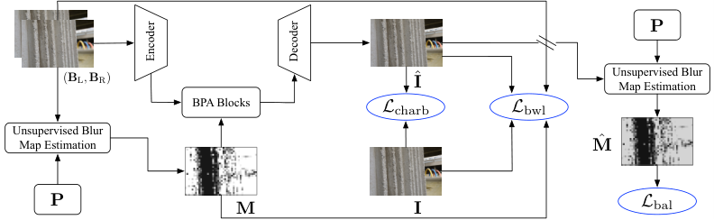
We first design a DP-aware prompt to adapt CLIP to output a blur map, , which quantizes disparity unsupervisedly between and . Then, we propose a BPA block based network which employs the blur map as deblurring priors to restore a sharp image from . To regularize the restoration of , a blur-weighting loss and a blur-aware loss are also introduced that were underpinned by our unsupervised blur map estimation strategy. The overall framework is shown in Fig. 2. Details are presented below.
3.1 Unsupervised Blur Map Estimation
Preliminary.
CLIP respectively embeds an image and a text description into a common semantic space of dimension with an image encoder and a text encoder, obtaining image embedding and text embedding . By optimizing a contrastive loss, the embeddings of the aligned image and text pair, , stay similar, i.e., maximizing the semantic similarity by , where is the cosine similarity metric. Meanwhile, the semantics of misaligned pairs, are pushed away from each other, i.e., . With comprehensive training data, CLIP can be leveraged to align images with pre-defined prompt templates composed of open-world text descriptions for zero-shot learning Radford et al. 2021.
For a DP pair, the disparity for a pixel in the left view is defined by its location and that of its corresponding pixel at in the right view.
In the literature, this DP disparity Punnappurath et al. 2020 is defined as
| (1) |
where and are the intensity of the two matching points, is a function of the radius of the circle of confusion, is the point depth, and and are lens-dependent constants Pan et al. 2021; Xin et al. 2021; Abuolaim et al. 2021; Garg et al. 2019.
Analysis.
Leveraging the CLIP, zero-shot blur map estimation can be generally divided into three steps. i) Image Encoding. Considering the image encoder of the CLIP is trained with monocular RGB images, a function is required to create a new monocular image from the DP image pair . To obtain the dense embedding for the blur map estimation task, we follow Zhang et al. 2022b to pop out the final pooling layer from the image encoder, yielding an embedding matrix , where and are the height and width for embedding of the newly created image, respectively. Mathematically, we have
| (2) |
Each pixel of has encoded the local semantic information for a corresponding region in . ii) Text Encoding. A text encoder is used to embed the semantics of a prompt describing the blur into the text embedding,
| (3) |
iii) Blur map estimation. Let be a -dimensional embedding at position of , , and . The embedding and the blur semantic-based text embedding are expected to be similar if the pixel at is blurred. Therefore, the blur mask of is obtained by
| (4) |
Note, normalizes the cosine similarity output to a probability space, to reflect the degree of blur at the position. Here, is sampled to have the same resolution as or , returning .
Given the analysis above, our goal is to develop text prompts , while adapting the function , to enable the use of semantic information from CLIP to generate the blur map in an unsupervised manner. In particular, we explore the blur-aware, DP-aware, and ensembling formats with detailed presented below.
Blur-aware Format.
An intuitive approach is setting a prompt that describes the blur to query a blur map , e.g., [A blurry image.]. The is then defined to synthesize a center view of the DP pair by averaging the left view and right view , as the average of two sub-images is equivalent to the image captured by a regular sensor Punnappurath et al. 2020; Abuolaim et al. 2022. However, the disparity information among the DP pair is neglected, resulting in a sub-optimal blur map. Refer to Fig. 4 for comparisons.
DP-aware Format.
Based on the DP image formation process, the disparity is proportional to the degree of blur exhibited in the DP view Abuolaim and Brown 2020. We thus propose to guide CLIP to understand the disparity exhibited between and which eventually leads to better mask () generation. To this end, we first formulate the disparity in the DP pair and then study the disparity-aware prompt and function designing. Such design leads us to query degrees of displacement between the left and right view from the CLIP, without any fine-tuning, to obtain the blur map .

Note that the CLIP is the vision-text alignment model trained with monocular image input. To extract the displacement between left/right views of the DP pair, we explore several input-prompt formats: i) Concatenating the left and right views horizontally, and prompting their difference, e.g., [The left and right of the image are different.]; ii) Prompting the horizontal symmetry between the left and right views, e.g., [A horizontally symmetric image.] (Fig. 3).


Empirically, we achieve the best performance with the second prompt format. When describing the symmetry in the prompt , we concatenate the left view with a horizontally flipped right view along the width axial in the . We then obtained image features . To transform to the same aspect ratio of and , we average the corresponding pixel-wise features based on the transformation in and have . For and , we define
| (5) |
Back to the left-hand side of Eq. 4, we have
| (6) |
Here, is the text embedding of the prompt describing symmetry. Note that the high similarity value, i.e. indicates pixels in sharp regions. Therefore the blur map is derived as in Eq. 6. Similarly, the is sampled to the same resolution of the DP pair, returning . For this blur map estimation strategy, we conclude the lemma below,
Lemma 3.1.
A pixel is sharp if and only if it is horizontally symmetric in the left view and the horizontally flipped right view, otherwise, the pixel is blurred.
Proof.
Following Eq. 1, we have being sharp, given . In other words, we have , demonstrating the horizontal symmetry. Reversely, the horizontal symmetry breaks once the disparity/blur occurs. ∎
Ensembling format.
Given the analysis that the degradations in the DP pair can be described by both the blurriness and symmetricity, we thus propose to obtain the mask by ensembling the blur-aware and DP-aware formats jointly. Please refer to Table 5 for details of the 8 prompts designed from blur-aware and DP-aware formats.
3.2 Network
We train an encoder-decoder based deblurring network for restoring the DP pair into a sharp image with the derived blur map . Our network consists of a backbone network based on Chen et al. 2022 and a BPA block to interleave with the backbone network layers. In particular, the BPA block uses the obtained blur map as deblur kernel prior to help the restoration of on the fly.
Self-attention.
The self-attention (SA) mechanism is widely used in the defocus deblurring tasks Zamir et al. 2022. We first briefly review it. Let be the intermediate feature embedding of a blur image from the backbone encoder, where , , are height, width, and channel of the feature. The self-attention is input with query , key , and value that are linearly projected from , and then calculate an attention map between and for adaptively aggregating . This process is defined as follows,
| (7) | ||||
| (8) |
where , , are learnable weight matrices, is a normalization factor that is typically set to the square root of the latent dimension, and is known as the attention map.
BPA Block.
The attention map can be considered as an adaptive deblur kernel prior for restoring the DP pair in the feature space. We are motivated to modulate the attention map by supplying the blur map , utilizing blur-related prior knowledge to additionally assign a deblur kernel for each region in to aggregate a sharp feature embedding from its neighboring regions. We re-write the Eq. 8 as
| (9) | ||||
| (10) |
and show that the restoration result is further improved in Fig. 5, where is a convolution-based feed forward layer that is used to learn a deblur kernel for each region of from the unnormalized blur map , resulting in . The function reshapes into , and pads the reshaped to , for shape alignment issue.


| Method | Outdoor Scenes | Indoor Scenes | Average | |||||||||
| PSNR↑ | SSIM↑ | MAE↓ | MSE_rel↓ | PSNR↑ | SSIM↑ | MAE↓ | MSE_rel↓ | PSNR↑ | SSIM↑ | MAE↓ | MSE_rel↓ | |
| EBDB | 25.77 | 0.772 | 0.040 | 0.051 | 21.25 | 0.599 | 0.058 | 0.086 | 23.45 | 0.683 | 0.049 | 0.067 |
| DMENet | 25.50 | 0.788 | 0.038 | 0.053 | 21.43 | 0.644 | 0.063 | 0.084 | 23.41 | 0.714 | 0.051 | 0.067 |
| DPDNet | 27.48 | 0.849 | 0.029 | 0.042 | 22.90 | 0.726 | 0.052 | 0.071 | 25.13 | 0.786 | 0.041 | 0.055 |
| RDPD | 28.10 | 0.843 | 0.027 | 0.039 | 22.82 | 0.704 | 0.053 | 0.072 | 25.39 | 0.772 | 0.040 | 0.053 |
| DDDNet | 27.57 | 0.833 | 0.030 | 0.041 | 23.28 | 0.708 | 0.050 | 0.068 | 25.36 | 0.768 | 0.041 | 0.054 |
| IFAN | 28.66 | 0.868 | 0.025 | 0.037 | 23.46 | 0.743 | 0.049 | 0.067 | 25.99 | 0.804 | 0.037 | 0.050 |
| BAMBNet | 28.60 | 0.872 | 0.026 | 0.037 | 24.30 | 0.772 | 0.045 | 0.060 | 26.40 | 0.821 | 0.036 | 0.047 |
| DeepRFT | 28.48 | 0.870 | 0.025 | 0.038 | 23.09 | 0.736 | 0.051 | 0.070 | 25.71 | 0.801 | 0.037 | 0.051 |
| Restormer | 29.48 | 0.895 | 0.023 | 0.034 | 23.97 | 0.773 | 0.047 | 0.063 | 26.66 | 0.833 | 0.035 | 0.046 |
| K3DN | 29.87 | 0.890 | 0.022 | 0.032 | 24.37 | 0.780 | 0.046 | 0.060 | 27.06 | 0.835 | 0.034 | 0.044 |
| Ours (Small) | 29.55 | 0.893 | 0.021 | 0.033 | 24.38 | 0.773 | 0.043 | 0.065 | 26.91 | 0.831 | 0.032 | 0.045 |
| Ours (Large) | 29.88 | 0.896 | 0.020 | 0.032 | 24.73 | 0.786 | 0.037 | 0.059 | 27.24 | 0.840 | 0.028 | 0.043 |
| Method | PSNR↑ | SSIM↑ | MAE↓ | MSE_rel↓ |
| EBDB | 26.48 | 0.683 | 0.036 | 0.047 |
| DMENet | 30.14 | 0.939 | 0.017 | 0.031 |
| DPDNet | 31.45 | 0.926 | 0.016 | 0.027 |
| RDPD | 32.42 | 0.912 | 0.016 | 0.024 |
| DDDNet | 33.21 | 0.956 | 0.010 | 0.022 |
| IFAN | 34.18 | 0.929 | 0.012 | 0.020 |
| BAMBNet | 35.90 | 0.954 | 0.012 | 0.016 |
| DeepRFT | 36.52 | 0.952 | 0.010 | 0.015 |
| Restormer | 36.44 | 0.957 | 0.010 | 0.015 |
| K3DN | 38.23 | 0.965 | 0.008 | 0.012 |
| Ours (Small) | 37.27 | 0.959 | 0.010 | 0.014 |
| Ours (Large) | 38.62 | 0.971 | 0.008 | 0.012 |
| Method | PSNR↑ | SSIM↑ | MAE↓ | MSE_rel↓ |
| EBDB | 24.23 | 0.637 | 0.031 | 0.054 |
| DMENet | 25.17 | 0.731 | 0.036 | 0.061 |
| DPDNet | 29.84 | 0.828 | 0.032 | 0.055 |
| RDPD | 31.09 | 0.861 | 0.025 | 0.028 |
| DDDNet | 30.14 | 0.840 | 0.016 | 0.031 |
| IFAN | 31.12 | 0.865 | 0.023 | 0.028 |
| BAMBNet | 31.78 | 0.867 | 0.016 | 0.026 |
| DeepRFT | 31.71 | 0.879 | 0.016 | 0.024 |
| Restormer | 32.27 | 0.871 | 0.016 | 0.024 |
| K3DN | 32.84 | 0.905 | 0.014 | 0.023 |
| Ours (Small) | 32.98 | 0.895 | 0.014 | 0.022 |
| Ours (Large) | 33.44 | 0.907 | 0.013 | 0.021 |
3.3 Network Training
We optimize our deblurring network with the widely used Charbonnier loss. Moreover, we propose a blur-aware loss and a blur weighting loss to penalize the blurred regions in the restoration .
Charbonnier loss.
We encourage the restoration to be close to the ground truth by using Charbonnier loss. We empirically set to , and define
| (11) |
Blur Weighting Loss.
We impose an adaptive penalty on the blurred regions of the DP pair , considering the degree of blur measured by CLIP. It encourages the network to focus on the restoration of heavily blurred regions. We first normalize the deviations between and by the deviations between and , and then re-use the blur map to select blurred regions residing in the DP pair.
| (12) |
where we use the blur map (with soft logits) to reflect the blur levels detected by CLIP.
Blur-aware Loss.
We encourage to be sharp by leveraging the versatile knowledge contained in the CLIP. We generate the blur map by the blur-aware format for the restoration, and penalize the blur exhibited in . Similar to , we use the unnormalized version of the blur map,
| (13) |
This encourages to be zero, i.e., no blur exists in the restoration.
Total Loss.
Our network is optimized by minimizing the following loss function
| (14) |
where is a normalization factor determinated by the image domain size , and and are hyperparameters to balance losses.
4 Experiments and Analysis
Implementation Details.
We implement our model under the PyTorch framework. We use the pre-trained and ViT-B/32 Dosovitskiy et al. 2021 architecture-based CLIP Radford et al. 2021 for our blur map estimation strategy. We train the deblurring network in two stages for steps in total with the Adam optimizer. In each stage, the learning rate is decayed from to by a cosine annealing strategy. In the first stage, we train the network for steps, and only use the Charbonnier loss . In the second stage, the network is finetuned for steps with , where we have and . More implementation details are given in our supplementary material.
Datasets.
Our method is evaluated on three real-world DP defocus deblurring datasets, DPD-blur dataset Abuolaim and Brown 2020 and DPD-disp dataset Punnappurath et al. 2020, and PixelDP dataset Xin et al. 2021. We follow Abuolaim and Brown 2020 on the training and testing splits. For the DPD-disp dataset and PixelDP dataset, we use them for testing only, re-using the checkpoints trained from the DPD-blur dataset as they do not provide ground-truth (GT) data or with limited dataset size. Moreover, two synthetic datasets, DDD-syn Pan et al. 2021 and RDPD Xin et al. 2021, are also used for evaluations.
Evaluation Metrics.
We use peak signal-to-noise ratio (PSNR), structural similarity (SSIM), mean absolute error (MAE), and relative mean squared error (MSE_rel) as our evaluation metrics.
Baseline Methods.
We compare with SOTA DP defocus deblurring methods, i.e., EBDB Karaali and Jung 2017, DMENet Lee et al. 2019, DPDNet Abuolaim and Brown 2020, RDPD Abuolaim et al. 2021, DDDNet Pan et al. 2021, IFAN Lee et al. 2021, BAMBNet Liang et al. 2022, DeepRFT Mao et al. 2023, Restormer Zamir et al. 2022, and K3DN Yang et al. 2023.
4.1 Comparisons with State-of-the-Art
Quantitative Comparison.
We compare with the state-of-the-art methods on the DPD-blur, DDD-syn, and RDPD datasets in Table 1, Table 3, and Table 3, respectively. We train our model with small and large configurations, and details are given in our supplementary material. Our observations are as follows: i) With our model (Small), we achieve similar restoration results with Restormer and K3DN, the third-best and second-best method, in all datasets. ii) When scaling to the large model, we consistently outperform all methods on all evaluation metrics. For example, our method, K3DN, and Restormer respectively achieve 27.24/27.06/26.66, 38.62/38.23/36.44, and 33.44/32.84/32.27 PSNR (dB) in the DPD-blur, DDD-syn, and RDPD datasets. Meanwhile, on a single RTX 4090 GPU, we remain to have a lower Infer. time (considering the frozen parameters in CLIP) which is 0.042s and 0.054s for our small and large models, while K3DN/Restormer takes 0.198s/0.255s.
Qualitative Comparison.
We compare with state-of-the-art methods on the DPD-blur dataset (Fig. 6). As shown, our method performs sharper and clearer restorations of edges and texts. To further demonstrate the benefits of using CLIP to generate the blur mask unsupervisedly in our approach, we provide an example in Fig. 7, which preserves sharp regions (e.g., text ‘York’) in the input blur image effectively compared to the second-best baseline.


| Blur-aware Prompt | DP-aware Prompt | |
| [A blurry image.] | [A symmetrical image.] | |
| [An obscured image.] | [A horizontally symmetrical image.] | |
| [An out of focus image.] | [A left-right symmetrical image.] | |
| [An image lacking sharpness.] | [A symmetrical image at the pixel level.] |
| Blur-aware Prompt | DP-aware Prompt | |||||||
| PSNR↑ | SSIM↑ | MAE↓ | MSE_rel↓ | PSNR↑ | SSIM↑ | MAE↓ | MSE_rel↓ | |
| 26.83 | 0.829 | 0.033 | 0.045 | 26.82 | 0.830 | 0.033 | 0.046 | |
| 26.81 | 0.829 | 0.033 | 0.046 | 26.83 | 0.830 | 0.032 | 0.046 | |
| 26.75 | 0.828 | 0.034 | 0.046 | 26.82 | 0.830 | 0.033 | 0.046 | |
| 26.77 | 0.829 | 0.033 | 0.046 | 26.85 | 0.830 | 0.032 | 0.045 | |
| Ens.1 | 26.80 | 0.829 | 0.033 | 0.046 | 26.84 | 0.830 | 0.032 | 0.046 |
| Ens.2 | 26.91 | 0.831 | 0.032 | 0.045 | 26.91 | 0.831 | 0.032 | 0.045 |
| Setting | PSNR↑ | SSIM↑ | MAE↓ | MSE_rel↓ |
| i) NAFNet | 26.21 | 0.817 | 0.038 | 0.049 |
| ii) Concat | 26.76 | 0.826 | 0.033 | 0.046 |
| iii) SA | 26.59 | 0.824 | 0.036 | 0.047 |
| iv) Concat + SA | 26.80 | 0.829 | 0.032 | 0.046 |
| v) BPA block | 26.91 | 0.831 | 0.032 | 0.045 |
| BPA block | Loss | PSNR↑ | SSIM↑ | MAE↓ | MSE_rel↓ |
| ✗ | 26.21 | 0.817 | 0.038 | 0.049 | |
| ✗ | 26.53 | 0.822 | 0.036 | 0.047 | |
| ✓ | 26.71 | 0.825 | 0.034 | 0.046 | |
| ✓ | + | 26.76 | 0.828 | 0.033 | 0.046 |
| ✓ | + | 26.81 | 0.829 | 0.032 | 0.046 |
| ✓ | 26.91 | 0.831 | 0.032 | 0.045 |
4.2 Ablation Study
We study model architecture, blur map estimation, and losses in this section. All experiments are performed in the DPD-blur dataset.
Ablation of Model Architecture.
We study the effective usage of blur map as prior knowledge for DP defocus deblurring (Tab. 6). To show the benefits of using blur maps, we consider four baselines: i) NAFNet Chen et al. 2022, the baseline model; ii) Concat, concatenating the blur map with the DP pair before feeding to the model; iii) SA, using the self-attention layer Dosovitskiy et al. 2021 in Eq. 8 to the model only; iv) Concat+SA, combines the Concat and SA settings; v) BPA block, using kernel priors from the blur map to assist deblurring. Our model consistently outperforms all baselines, which indicates the effectiveness of using the blur map.
Ablation of Losses.
We investigate the proposed blur weighting loss and blur-aware loss (Tab. 7) with a baseline as the setting. We first use and to our baseline, NAFNet (i.e., not using our BPA block), that only uses , having 0.32 PSNR (dB) improvements. Secondly, we train our model (backbone + BPA block) with Charbonnier loss, resulting in 26.71/0.825 higher PSNR (dB)/SSIM. By using the or , we respectively achieve 0.05/0.003 or 0.10/0.004 higher PSNR (dB)/SSIM. Combining all losses, we have the best restoration performance at 26.91/0.831 for PSNR (dB)/SSIM. Moreover, we verify the generalization ability of our and losses on state-of-the-art networks, improving PSNR of Restormer and DeepRFT by 0.25 and 0.41 PSNR (dB). Refer to our supplementary materials for details.
Ablation of Blur Map Estimation.
We ablate with different prompts used to generate the blur map. The blur-aware and DP-aware prompts are presented in Tab. 5, and we show their impact on model performance with Tab. 5. We then ensemble the groups of blur-aware prompt and disparity-aware prompt individually (Ens.1), leading to 26.80dB/0.829 and 26.84/0.830 PSNR (dB)/SSIM. By ensembling all prompts (Ens.2), we have 26.91/0.831 PSNR (dB)/SSIM, consistently outperforming other approaches of generating blur masks. More ablations and analyses of CLIP can be found in our supplementary material.
4.3 Discussion and Limitation
Discussion.
The reader may wonder about the performance of our unsupervised blur map estimation strategy. Therefore, we perform two qualitative evaluations on the DPD-disp dataset, where the GT disparity is included. We compare with BAMBNet Liang et al. 2022 and DPD-disp Punnappurath et al. 2020.
First, we consider blur map estimation. To obtain the GT blur map, the pixel with disparity that satisfies is used as the sharp pixel, reversely, it is a burred pixel. Our method, BAMBNet and DPD-disp Liang et al. 2022 respectively have 89.8%/70.2%/88.3% accuracy (the higher, the better, details are in the supplementary material), showing the effectiveness of our method.
Second, we explore disparity estimation. The logits of our unnormalized blurred map are potentially linearly correlated with the ground-truth disparity. Therefore, we compare with the state-of-the-art DP disparity estimation method, DPD-disp Punnappurath et al. 2020. Following Punnappurath et al. 2020, we use AI(1), AI(2), and as the evaluation metrics (the lower, the better). The AI(1), AI(2), and of our method, BAMBNet, and DPD-disp are 0.063/0.106/0.069, 0.130/0.184/0.096, 0.306/0.772/0.0159. Though our blur map is estimated with a single forward pass, we still achieve a reasonable performance in the disparity estimation. This potentially explains the high performance of our DP defocus deblurring network, as obtaining the disparity prior benefits the defocus task.
Limitation.
As the image encoder of CLIP is trained under a classification-alike pre-training task, it will focus more on local details that help identify its scene class. Textureless regions would produce non-significant semantic reactions, e.g., large areas of wall, ceiling, or floor, and reduce the quality of the estimated blur map. It is possible to use a vision language framework that drives more sensitivity to regions with less texture.
More.
In the supplementary material, more qualitative and quantitative evaluations, ablation studies, and analysis are provided, as well as results that our framework is being generalized to restoring single images with defocus blur or motion blur tasks.
5 Conclusion and Broader Impact
In this paper, we study end-to-end defocus deblurring of DP images, leveraging the blur-related prior knowledge from the CLIP. We first estimate a blur map with an ensemble of blur-aware and DP-aware strategies, and then use the estimated blur map as the deblurring kernel prior to restoring the DP image. We also propose a blur-aware and blur-weighting loss to regularize the restorations of the DP images during training, by distilling the knowledge of blur from CLIP. In extensive experiments, our method outperforms past works by a large margin in quantitative and qualitative restoration performance.
Broader Impact.
The proposed DP-aware strategy is promising to apply and extend CLIP to diverse zero-shot stereo vision tasks. We hope it will motivate future work.
References
- Abuolaim and Brown (2020) Abdullah Abuolaim and Michael S Brown. Defocus deblurring using dual-pixel data. In European Conference on Computer Vision, pages 111–126. Springer, 2020.
- Abuolaim et al. (2021) Abdullah Abuolaim, Mauricio Delbracio, Damien Kelly, Michael S Brown, and Peyman Milanfar. Learning to reduce defocus blur by realistically modeling dual-pixel data. In Proceedings of the IEEE/CVF International Conference on Computer Vision, pages 2289–2298, 2021.
- Abuolaim et al. (2022) Abdullah Abuolaim, Mahmoud Afifi, and Michael S Brown. Improving single-image defocus deblurring: How dual-pixel images help through multi-task learning. In Proceedings of the IEEE/CVF Winter Conference on Applications of Computer Vision, pages 1231–1239, 2022.
- Auty and Mikolajczyk (2023) Dylan Auty and Krystian Mikolajczyk. Learning to prompt clip for monocular depth estimation: Exploring the limits of human language. In Proceedings of the IEEE/CVF International Conference on Computer Vision, pages 2039–2047, 2023.
- Chen et al. (2022) Liangyu Chen, Xiaojie Chu, Xiangyu Zhang, and Jian Sun. Simple baselines for image restoration. In Computer Vision–ECCV 2022: 17th European Conference, Tel Aviv, Israel, October 23–27, 2022, Proceedings, Part VII, pages 17–33. Springer, 2022.
- Choi et al. (2023) Myungsub Choi, Hana Lee, and Hyong-euk Lee. Exploring positional characteristics of dual-pixel data for camera autofocus. In Proceedings of the IEEE/CVF International Conference on Computer Vision, pages 13158–13168, 2023.
- Deng et al. (2009) Jia Deng, Wei Dong, Richard Socher, Li-Jia Li, Kai Li, and Li Fei-Fei. Imagenet: A large-scale hierarchical image database. In 2009 IEEE conference on computer vision and pattern recognition, pages 248–255. IEEE, 2009.
- Dosovitskiy et al. (2021) Alexey Dosovitskiy, Lucas Beyer, Alexander Kolesnikov, Dirk Weissenborn, Xiaohua Zhai, Thomas Unterthiner, Mostafa Dehghani, Matthias Minderer, Georg Heigold, Sylvain Gelly, et al. An image is worth 16x16 words: Transformers for image recognition at scale. In International Conference on Learning Representations, 2021.
- Garg et al. (2019) Rahul Garg, Neal Wadhwa, Sameer Ansari, and Jonathan T Barron. Learning single camera depth estimation using dual-pixels. In Proceedings of the IEEE/CVF International Conference on Computer Vision, pages 7628–7637, 2019.
- Hu et al. (2023) Xueting Hu, Ce Zhang, Yi Zhang, Bowen Hai, Ke Yu, and Zhihai He. Learning to adapt clip for few-shot monocular depth estimation. arXiv preprint arXiv:2311.01034, 2023.
- Huang et al. (2023) Tianyu Huang, Bowen Dong, Yunhan Yang, Xiaoshui Huang, Rynson WH Lau, Wanli Ouyang, and Wangmeng Zuo. Clip2point: Transfer clip to point cloud classification with image-depth pre-training. In Proceedings of the IEEE/CVF International Conference on Computer Vision, pages 22157–22167, 2023.
- Karaali and Jung (2017) Ali Karaali and Claudio Rosito Jung. Edge-based defocus blur estimation with adaptive scale selection. IEEE Transactions on Image Processing, 27(3):1126–1137, 2017.
- Kim et al. (2023) Donggun Kim, Hyeonjoong Jang, Inchul Kim, and Min H Kim. Spatio-focal bidirectional disparity estimation from a dual-pixel image. In Proceedings of the IEEE/CVF Conference on Computer Vision and Pattern Recognition, pages 5023–5032, 2023.
- Lee et al. (2019) Junyong Lee, Sungkil Lee, Sunghyun Cho, and Seungyong Lee. Deep defocus map estimation using domain adaptation. In Proceedings of the IEEE/CVF Conference on Computer Vision and Pattern Recognition, pages 12222–12230, 2019.
- Lee et al. (2021) Junyong Lee, Hyeongseok Son, Jaesung Rim, Sunghyun Cho, and Seungyong Lee. Iterative filter adaptive network for single image defocus deblurring. In Proceedings of the IEEE/CVF Conference on Computer Vision and Pattern Recognition, pages 2034–2042, 2021.
- Li et al. (2022) Yu Li, Yaling Yi, Dongwei Ren, Qince Li, and Wangmeng Zuo. Learning dual-pixel alignment for defocus deblurring. arXiv preprint arXiv:2204.12105, 2022.
- Li et al. (2023) Yu Li, Dongwei Ren, Xinya Shu, and Wangmeng Zuo. Learning single image defocus deblurring with misaligned training pairs. In Proceedings of the AAAI Conference on Artificial Intelligence, pages 1495–1503, 2023.
- Liang et al. (2022) Pengwei Liang, Junjun Jiang, Xianming Liu, and Jiayi Ma. Bambnet: A blur-aware multi-branch network for dual-pixel defocus deblurring. IEEE/CAA Journal of Automatica Sinica, 9(5):878–892, 2022.
- Liang et al. (2023) Zhexin Liang, Chongyi Li, Shangchen Zhou, Ruicheng Feng, and Chen Change Loy. Iterative prompt learning for unsupervised backlit image enhancement. In Proceedings of the IEEE/CVF International Conference on Computer Vision, pages 8094–8103, 2023.
- Mao et al. (2023) Xintian Mao, Yiming Liu, Fengze Liu, Qingli Li, Wei Shen, and Yan Wang. Intriguing findings of frequency selection for image deblurring. In Proceedings of the 37th AAAI Conference on Artificial Intelligence, 2023.
- Monin et al. (2023) Sagi Monin, Sagi Katz, and Georgios Evangelidis. Continuous cost aggregation for dual-pixel disparity extraction. arXiv preprint arXiv:2306.07921, 2023.
- Pan et al. (2021) Liyuan Pan, Shah Chowdhury, Richard Hartley, Miaomiao Liu, Hongguang Zhang, and Hongdong Li. Dual pixel exploration: Simultaneous depth estimation and image restoration. In Proceedings of the IEEE/CVF Conference on Computer Vision and Pattern Recognition, pages 4340–4349, 2021.
- Punnappurath et al. (2020) Abhijith Punnappurath, Abdullah Abuolaim, Mahmoud Afifi, and Michael S Brown. Modeling defocus-disparity in dual-pixel sensors. In 2020 IEEE International Conference on Computational Photography (ICCP), pages 1–12. IEEE, 2020.
- Quan et al. (2023a) Yuhui Quan, Zicong Wu, and Hui Ji. Neumann network with recursive kernels for single image defocus deblurring. In Proceedings of the IEEE/CVF Conference on Computer Vision and Pattern Recognition, pages 5754–5763, 2023a.
- Quan et al. (2023b) Yuhui Quan, Xin Yao, and Hui Ji. Single image defocus deblurring via implicit neural inverse kernels. In Proceedings of the IEEE/CVF International Conference on Computer Vision, pages 12600–12610, 2023b.
- Radford et al. (2021) Alec Radford, Jong Wook Kim, Chris Hallacy, Aditya Ramesh, Gabriel Goh, Sandhini Agarwal, Girish Sastry, Amanda Askell, Pamela Mishkin, Jack Clark, et al. Learning transferable visual models from natural language supervision. In International conference on machine learning, pages 8748–8763. PMLR, 2021.
- Rao et al. (2022) Yongming Rao, Wenliang Zhao, Guangyi Chen, Yansong Tang, Zheng Zhu, Guan Huang, Jie Zhou, and Jiwen Lu. Denseclip: Language-guided dense prediction with context-aware prompting. In Proceedings of the IEEE/CVF Conference on Computer Vision and Pattern Recognition, pages 18082–18091, 2022.
- Shi and Yang (2023) Cheng Shi and Sibei Yang. Edadet: Open-vocabulary object detection using early dense alignment. In Proceedings of the IEEE/CVF International Conference on Computer Vision, pages 15724–15734, 2023.
- Son et al. (2021) Hyeongseok Son, Junyong Lee, Sunghyun Cho, and Seungyong Lee. Single image defocus deblurring using kernel-sharing parallel atrous convolutions. In 2021 IEEE/CVF International Conference on Computer Vision, ICCV 2021, Montreal, QC, Canada, October 10-17, 2021, pages 2622–2630. IEEE, 2021.
- Xin et al. (2021) Shumian Xin, Neal Wadhwa, Tianfan Xue, Jonathan T Barron, Pratul P Srinivasan, Jiawen Chen, Ioannis Gkioulekas, and Rahul Garg. Defocus map estimation and deblurring from a single dual-pixel image. In Proceedings of the IEEE/CVF International Conference on Computer Vision, pages 2228–2238, 2021.
- Yang et al. (2023) Yan Yang, Liyuan Pan, Liu Liu, and Miaomiao Liu. K3dn: Disparity-aware kernel estimation for dual-pixel defocus deblurring. In Proceedings of the IEEE/CVF Conference on Computer Vision and Pattern Recognition (CVPR), pages 13263–13272, 2023.
- Zamir et al. (2022) Syed Waqas Zamir, Aditya Arora, Salman Khan, Munawar Hayat, Fahad Shahbaz Khan, and Ming-Hsuan Yang. Restormer: Efficient transformer for high-resolution image restoration. In Proceedings of the IEEE/CVF Conference on Computer Vision and Pattern Recognition, pages 5728–5739, 2022.
- Zhang et al. (2022a) Renrui Zhang, Ziyu Guo, Wei Zhang, Kunchang Li, Xupeng Miao, Bin Cui, Yu Qiao, Peng Gao, and Hongsheng Li. Pointclip: Point cloud understanding by clip. In Proceedings of the IEEE/CVF Conference on Computer Vision and Pattern Recognition, pages 8552–8562, 2022a.
- Zhang et al. (2022b) Renrui Zhang, Ziyao Zeng, Ziyu Guo, and Yafeng Li. Can language understand depth? In Proceedings of the 30th ACM International Conference on Multimedia, pages 6868–6874, 2022b.
- Zhang et al. (2020) Yinda Zhang, Neal Wadhwa, Sergio Orts-Escolano, Christian Häne, Sean Fanello, and Rahul Garg. Du2net: Learning depth estimation from dual-cameras and dual-pixels. In European Conference on Computer Vision, pages 582–598, 2020.
- Zhou et al. (2023) Ziqin Zhou, Yinjie Lei, Bowen Zhang, Lingqiao Liu, and Yifan Liu. Zegclip: Towards adapting clip for zero-shot semantic segmentation. In Proceedings of the IEEE/CVF Conference on Computer Vision and Pattern Recognition, pages 11175–11185, 2023.